Article

Convolutional-Transformer Model with Long-Range Temporal Dependencies for Bearing Fault Diagnosis Using Vibration Signals

by
Hosameldin O. A. Ahmed
1,2 and
Asoke K. Nandi
2,3,*
1
OpenAITech Ltd., Old Marylebone, London NW1 5RA, UK
2
Department of Electronic and Electrical Engineering, Brunel University London, Uxbridge UB8 3PH, UK
3
School of Mechanical Engineering, Xi’an Jiaotong University, Xi’an 710049, China
*
Author to whom correspondence should be addressed.
Machines 2023, 11(7), 746; https://doi.org/10.3390/machines11070746
Submission received: 3 July 2023 / Revised: 11 July 2023 / Accepted: 14 July 2023 / Published: 17 July 2023

Abstract

:
Fault diagnosis of bearings in rotating machinery is a critical task. Vibration signals are a valuable source of information, but they can be complex and noisy. A transformer model can capture distant relationships, which makes it a promising solution for fault diagnosis. However, its application in this field has been limited. This study aims to contribute to this growing area of research by proposing a novel deep-learning architecture that combines the strengths of CNNs and transformer models for effective fault diagnosis in rotating machinery. Thus, it captures both local and long-range temporal dependencies in the vibration signals. The architecture starts with CNN-based feature extraction, followed by temporal relationship modelling using the transformer. The transformed features are used for classification. Experimental evaluations are conducted on two datasets with six and ten health conditions. In both case studies, the proposed model achieves high accuracy, precision, recall, F1-score, and specificity all above 99% using different training dataset sizes. The results demonstrate the effectiveness of the proposed method in diagnosing bearing faults. The convolutional-transformer model proves to be a promising approach for bearing fault diagnosis. The method shows great potential for improving the accuracy and efficiency of fault diagnosis in rotating machinery.

1. Introduction

The presence of complex and costly machinery in critical business operations needs effective condition monitoring and maintenance programs. Unforeseen failures can result in downtime, accidents, and financial losses. Maintenance operating expenses can range from 15% to 60% of production costs depending on the industry. To maintain a stable and healthy rotating machine, essential components, such as motors, bearings, gearboxes, etc., must operate effectively. Maintenance ensures their health condition by repairing, modifying, or replacing them. Rolling bearings play a critical role in the smooth functioning of rotating machinery by enabling motion between static and moving parts. Their failures may lead to major issues, accounting for 40–90% of machine failures [1]. Maintenance can be achieved through corrective and preventive approaches. Corrective maintenance is expensive, especially for large-scale applications, and performed after machine failure. Preventive maintenance incorporates time-based maintenance (TBM) and condition-based maintenance (CBM) methods, such as localised CBM or remote CBM. While TBM is costly and may not prevent failures, CBM is considered efficient, as 99% of equipment failures are preceded by non-specific conditions. CBM relies on condition monitoring (CM) to detect faults early, leading to accurate maintenance decisions. Vibration-based CM is extensively used due to its capability to analyse machine health without physical involvement [1,2,3,4].
CM for machinery usually includes both fault detection and diagnosis. Fault detection in CM intends to recognise deviations from normal operating conditions or predefined thresholds. It involves the comparison of measured data or signals with expected or reference values. When a fault is detected, further analysis is conducted to diagnose the root cause of the fault. Fault diagnosis in CM aims to identify the source of the fault. It encompasses analysing the acquired data and using techniques, such as signal processing, pattern recognition, statistical analysis, and machine learning algorithms, to identify the fault type. Rolling bearing faults generate periodic impulses known as the bearing fundamental defect frequency (BFDF). BFDF depends on fault location, bearing geometry, and shaft speed. Figure 1 [5] illustrates this. BFDFs are categorised as bearing pass frequency of the inner race (BPFI), bearing pass frequency of the outer race (BPFO), ball spin frequency (BSF), and fundamental train frequency (FTF), which describe the defects in the outer race, inner race, rolling element, and cage [6]. Equations that express these frequencies are as follows.
B P F I = N b S s h 2 1 + d b D p c o s φ
B P F O = N b S s h 2 1 d b D p c o s φ
B S F = D p 2 d b 1 d b D p c o s φ 2
F T F = S s h 2 1 d b D p c o s φ
Here φ is the load angle, D p is the pitch diameter, d b is the rolling element diameter, S s h is the shaft speed, and N b is the number of rolling elements. The vibration signal frequency indicates the fault cause, while the amplitude reflects the fault severity.
Vibration-based machine fault diagnosis is a challenging task due to the presence of noises and vibration signals from multiple sources within the collected data. Feature extraction methods are used to extract useful information from the raw vibration signals, which can then be used to classify the health condition of the machine using machine learning classifiers. The generalisability of the much-published research in this field has focused on analysing specific characteristics of the collected vibration signals in three domains: time, frequency, and time-frequency. Techniques within these domains can effectively obtain the essential information of the signal. Machine learning methods can then be employed to classify the health condition of a machine based on these computed features. The key assumption is that by carefully formulating these features, a machine-learning model can be trained to achieve high accuracy in classifying the machine’s health condition. For example, previous studies have proposed various techniques that use multiple statistical features extracted from the time domain. These features include mean, crest factor, peak-to-peak value, variance, root mean square (RMS), kurtosis, and skewness. Additionally, advanced techniques such as autoregressive moving average (ARMA), time synchronous averaging (TSA), filtering techniques, blind source separation (BSS), and stochastic parameters [1,7,8,9,10,11,12]. Also, numerous research studies have confirmed that employing frequency domain techniques enables the extraction of valuable insights from time series vibration signals by examining their frequency characteristics, which may not be easily discernible in the time domain. The fast Fourier transform (FFT) is a commonly used method of converting time-domain vibration signals into the frequency domain [13]. Furthermore, different characteristics derived from the vibration frequency spectrum have been employed to represent the health condition of machines. These include high-frequency resonance, high-order spectra, arithmetic mean, and the RMS of spectral difference techniques [14,15,16]. Additionally, several techniques operating in the time-frequency domain have been employed for analysing non-stationary vibration signals that often arise during machinery faults. These techniques comprise the short-time Fourier transform (STFT), Hilbert-Huang transform (HHT), wavelet transform (WT), empirical mode decomposition (EMD), local mean decomposition (LMD), and others [16,17,18,19,20,21].
Over the past two decades, there has been significant progress in the application of feature-learning techniques for automatically deriving meaningful representations from time series datasets. Previous studies in the field of vibration fault diagnosis have principally focused on exploring deep-learning methods, specifically deep neural networks (DNNs) and convolutional neural networks (CNNs), recurrent neural networks (RNNs), autoencoders, generative-adversarial networks (GANs), deep-belief networks (DBNs), and transfer learning for this purpose [22,23,24,25,26,27,28,29,30,31]. These techniques use hierarchical multi-layer data processing architectures to learn representations of the data. Additionally, the application of deep learning has initiated a renewed interest in transforming the 1D vibration signal into a 2D image, as inspired by recent developments in computer vision. This conversion allows for the exploration of discriminative characteristics present in the vibration signal [32].
Furthermore, the attention mechanism (AM) has recently developed as an effective tool in the field of intelligent fault diagnosis, bringing significant advantages through its internal correlation and global information extraction capabilities. This technique has been proposed to enhance the performance of various other models, contributing to their overall effectiveness. According to [33], the utilisation of AM in the field of intelligent fault diagnosis can be classified into three primary categories: recurrent-based, convolution-based, and self-attention-based methods. For example, Li et al. proposed a fault diagnosis method for rolling element bearings using deep learning with a bi-directional LSTM and an attention mechanism. The method effectively identifies informative data segments, extracts discriminative features, and visualises diagnostic knowledge. Experimental results on a rolling bearing dataset demonstrate its effectiveness with limited training data [34]. In [35], an approach using improved multi-scale coarse-grained convolutional neural networks with feature attention is introduced. It enables accurate fault diagnosis of rolling bearings in complex scenarios by directly processing raw vibration signals. Yang et al. propose a method for enhancing interpretability in fault diagnosis of neural networks. It combines multilayer bidirectional gated recurrent units, an attention mechanism, and convolution neural networks. Experimental results on bearings demonstrate the effectiveness of the model in localising discriminative information and understanding feature extraction in neural networks, particularly for mechanical vibration signals [36]. In [37], a model called AMMFN that combines a central network and multiple branch networks using inception networks is presented. The proposed model automatically extracts deep features from single-sensor data and enhances the information interaction and hierarchical fusion in multi-sensor data.
Additionally, an attention-based fusion strategy captures more correlation information, leading to improved accuracy and generalisation ability compared to other methods. Moreover, an early fault detection method for rolling bearings called MCNN-AGRU is proposed. In this method, a multiscale convolutional neural network is used for data processing and employs a gated recurrent unit network with an attention mechanism for prediction. The method detects early faults by comparing actual and predicted values using a reconstruction error [38]. In [39], a fault diagnosis technique called MSA-ResNet utilising a multi-scale attention mechanism in a residual network is introduced. The technique introduces an attention mechanism block for constructing new residual block combinations. It also incorporates a multi-scale structure through appropriate convolution kernel sizes. The MSA-ResNet algorithm enhances feature sensitivity, extracts multi-scale features from complex mechanical vibration signals, and achieves an effective diagnosis of rolling bearing faults. Experimental results on bearing datasets demonstrate the method’s advantages for multi-scale feature extraction, noise immunity, and fault classification accuracy. Moreover, a multi-scale attention-mechanism-based convolutional neural network (MSAM-CNN), which is a 1D neural network with attention and convolutional layers for rolling bearing fault diagnosis, is proposed. It processes vibration signals on various scales using parallel branches, fusing complementary features, and utilising an attention mechanism for optimal feature selection [40].
Moreover, recent research has highlighted the inherent capabilities of the transformer model introduced in [41] to capture distant relationships. The transformer represents a sequence transduction model that relies entirely on attention, thereby replacing the conventional recurrent layers found in encoder-decoder architectures with multi-headed self-attention. However, there have been few attempts to investigate the application of the transformer model for fault diagnosis. For example, Hou et al. introduced a diagnosisformer model, which is an attention-based multi-feature parallel fusion approach for rolling bearing fault diagnosis. The model utilises the transformer architecture as its fundamental network. The process begins by extracting frequency domain features from the original data through an FFT. Subsequently, normalisation operations and embeddings are applied to prepare the model input. Next, a multi-feature parallel fusion encoder is employed to extract both local and global features from the bearing data. These extracted features are then passed to a cross-flipped decoder, followed by a classification head for fault classification [42]. In [43], a method for diagnosing bearing faults is presented. The method combines the joint feature extraction of a transformer and a residual neural network (ResNet) with transfer learning (TL). In this method, first, the data is fed into both the transformer encoder and the ResNet architecture. The encoder extracts features and word embeddings through a one-dimensional convolutional layer. The resulting feature sequences from the encoder and ResNet are then combined and classified. Additionally, a TL strategy with model fine-tuning is employed to alleviate the training complexity of the proposed method for new tasks.
In [44], a transformer model based on mask self-supervised learning, for diagnosing bearing faults in multistage centrifugal fans within petrochemical units with limited samples, is presented. The proposed method utilises mask self-supervised learning (SSL) to extract robust representations of fault signals and discover potential relationships among subsequences. This process allows for the pretraining of a model with well-generalised parameters using unlabelled samples. Consequently, a small set of labelled samples is employed for fine-tuning through supervised learning, enabling the proposed method to possess the discriminative capability required for identifying various types of bearing faults. Additionally, Wu et al. proposed a classifier based on the transformer architecture, designed to effectively detect various known fault types and their severity levels, while also identifying novel fault conditions. The proposed method involves transforming raw vibration signals into time-frequency spectrograms, which are then used as input for the classifier. In this method, using the classifier’s advanced feature extraction performance, a technique based on Mahalanobis distance is employed to determine whether a fault originates from a previously unseen condition. In the event a novel fault is detected, the model is retrained using the novel data following an incremental learning approach [45].
To date, the utilisation of the transformer model in the field of fault diagnosis is currently in an early stage of investigation. This study aims to contribute to this growing area of research by proposing a novel deep-learning architecture that combines the strengths of CNNs and transformer models for effective fault diagnosis in rotating machinery. The proposed method follows a sequential approach. It starts with extracting features from the vibration signals utilising CNNs, followed by temporal relationship modelling using the transformer model. The transformed features are used by the classifier to diagnose bearing faults effectively. By incorporating local and long-range temporal dependencies in vibration signals, this method successfully diagnoses bearing faults. The combination of the CNN’s feature extraction and the transformer model classification improves their strengths, leading to accurate fault diagnoses. The main contributions of this paper are as follows:
  • Novel Deep-Learning Architecture: This method introduces a unique deep-learning architecture that combines CNNs and transformer models to enhance fault diagnosis in rotating machinery. This architecture contributes to this growing area of research by utilising the strengths of both components.
  • Sequential Approach: The proposed method offers a systematic and sequential approach to fault diagnosis. It begins with the normalisation of vibration signals, efficiently addressing scale differences. Then, CNNs are employed for feature extraction, capturing important characteristics of the signals. Afterward, transformer models are used to model temporal relationships. This systematic process ensures a comprehensive analysis of the vibration signals.
  • Effective Feature Extraction and Temporal Relationship Modelling: Using CNNs, this approach excels at extracting key features from vibration signals, enabling an accurate diagnosis of bearing faults. Incorporating transformer models enables the modelling of long-range temporal dependencies, capturing dynamic patterns, and relationships over extended time intervals for a deeper understanding of fault behaviours and improved diagnosis performance.
  • Incorporation of Local and Long-Range Temporal Dependencies: By incorporating both local and long-range temporal dependencies in vibration signals, the method successfully captures the complex patterns and variations associated with bearing faults. This inclusion enhances the diagnostic accuracy and robustness of the model.
  • Improvement of CNN and Transformer Model Strengths: The combination of CNNs for feature extraction and transformer models for the modelling of long-range temporal dependencies improves their individual strengths. CNNs efficiently extract discriminative features from the vibration signals, while transformer models excel at modelling long-range temporal relationships. The fusion of these two components enhances the overall performance of the fault diagnosis model, leading to precise fault diagnoses.
The remainder of this paper is organised as follows. Section 2 describes the proposed method. Section 3 is devoted to descriptions of the experimental study used to validate the proposed method and presents comparison results. Finally, Section 4 offers some conclusions.

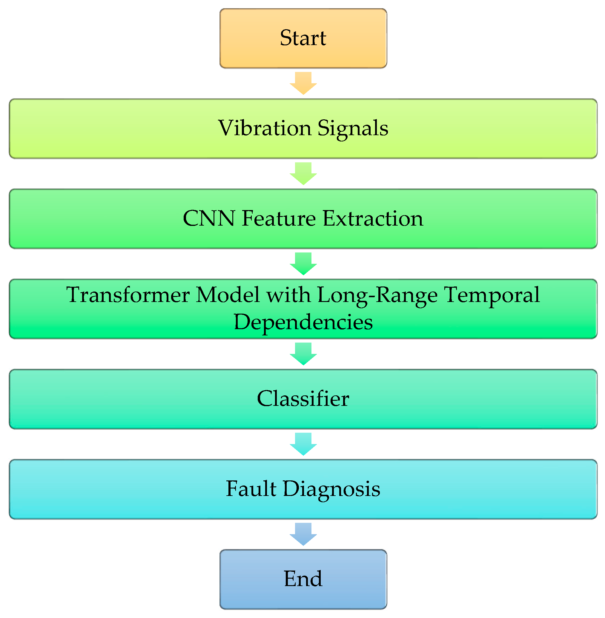
2. The Proposed Method

In this section, we introduce the convolutional-transformer model with long-range temporal dependencies for bearing fault classification. The proposed method is a novel deep-learning architecture that combines the advantages of CNNs and the transformer model. The architecture of the proposed method is shown in Figure 2. This architecture represents the sequential steps involved in the proposed method. Starting with the vibration signal, the proposed method applies the CNNs’ feature extraction to capture relevant features. The extracted features are then processed by the transformer, which models the temporal relationships. The transformed features are fed into the classifier for fault diagnosis. The proposed method aims to utilise both local and long-range temporal dependencies in the bearing vibration signals, leading to efficient fault diagnosis in rotating machinery. In this method, the combination of the CNN’s feature extraction and the temporal transformer improves the strengths of both techniques to efficiently diagnose bearing faults. The CNN is well-suited for extracting local features from vibration signals, while the temporal transformer can capture long-range temporal dependencies and patterns to make accurate fault diagnoses. The following sections provide a more detailed overview of the proposed method.

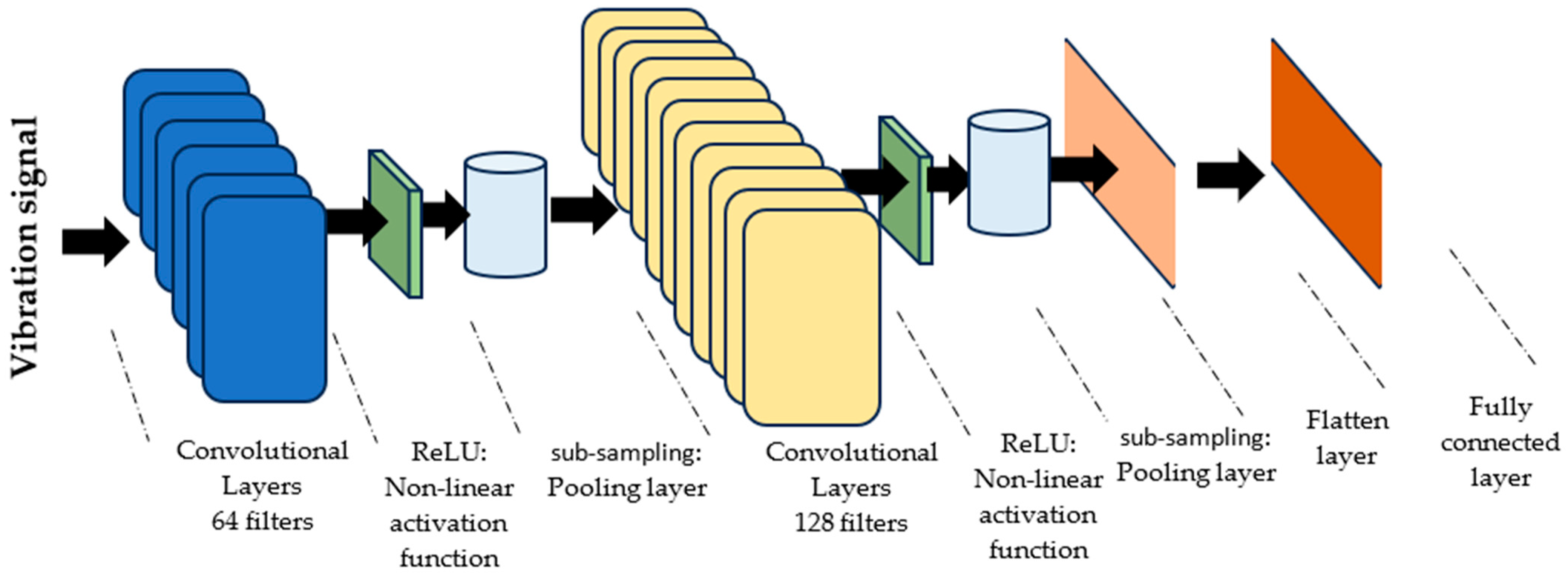
2.1. CNN Feature Extraction

The CNN, also referred to as a convNet, is a multi-stage neural network that typically consists of an input layer, convolutional layers, sub-sampling (or pooling) layers, fully connected layers, and an output layer. CNNs are designed to perform feature learning, where they learn meaningful features by iteratively applying convolutional layers, activation layers, and pooling processes to the input data. These procedures enable the network to learn distinctive characteristics from the provided data. The convolution layers perform convolution operations by applying various local filters to the raw input data, resulting in the generation of invariant local features. Simultaneously, the pooling layers extract the most important features from the convolved data [27,46]. Mathematically, the convolution computation can be expressed as follows:
h j = f ( i X i W i j + b j ) ,
In this equation, we have h j as the j-th output feature map of the current convolutional layer. X i represents the i-th output feature of the previous convolutional layer. The symbol ∗ denotes the convolution operator. W i j is the mapping of the convolution kernel that connects the c input feature map to the j-th output feature map in the current layer. The term b j refers to the bias associated with the j-th feature kernel and f represents the activation function. The widely utilised activation function in neural networks is the rectified linear unit (ReLU), which can be mathematically represented as follows:
f x = 0 ,   i f   x < 0 x ,     i f   x 0 ,
The pooling layer is responsible for performing nonlinear down-sampling to decrease the output dimensionality. It achieves this by employing various pooling techniques, including maximum pooling, averaging pooling, and random pooling. Among these techniques, maximum pooling is frequently used and can be mathematically described by Equation (7).
X j = f ( α j d o w n ( X i ) + b j ) ,
Here, X j denotes the j-th output obtained from the current pooling layer. The constant α j is utilised to regulate the extent of data modification performed by the pooling layer. The function d o w n ( X i ) corresponds to the down-sampling process applied to the i-th output originating from the preceding layer. b j signifies the bias associated with the j-th feature kernel used in the present pooling layer. Lastly, the f represents the activation function. The architecture of the proposed CNN feature extractor is presented in Figure 3.

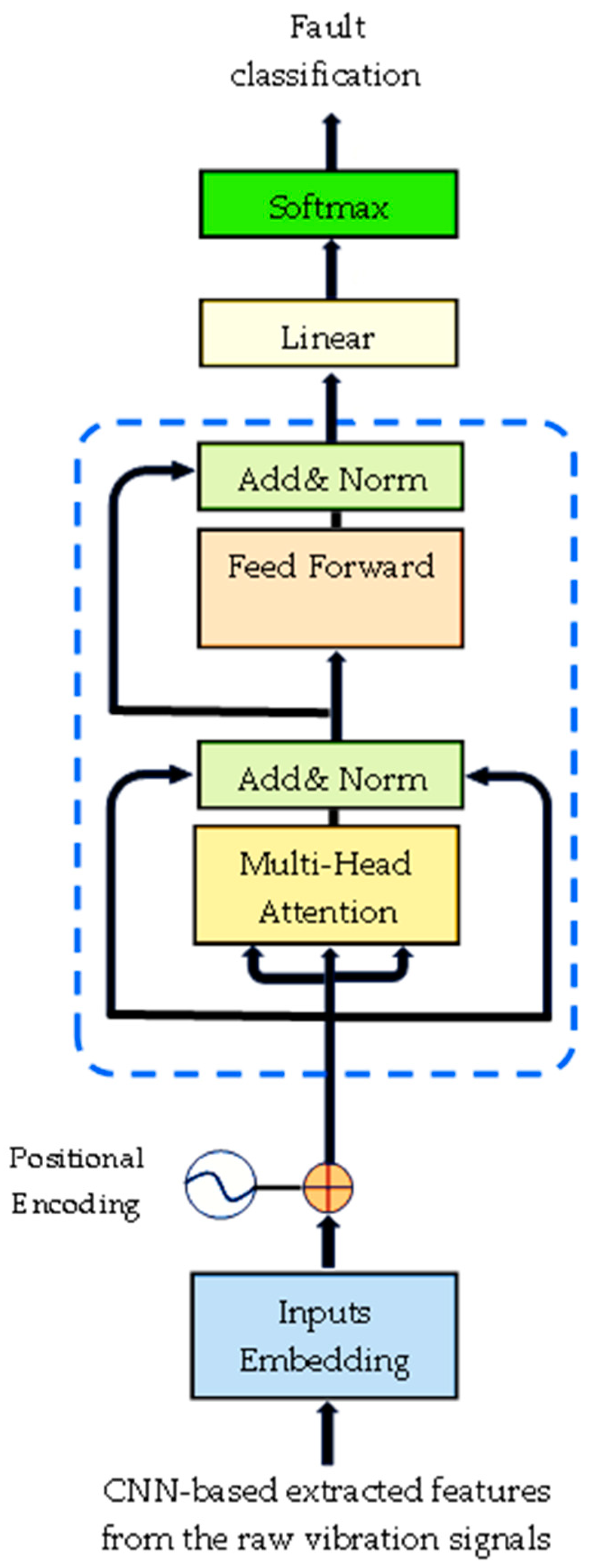
2.2. Temporal Transformer

The transformer architecture can be described as a combination of encoder and decoder components, organised in a stacked manner [41]. Figure 4 illustrates the overall structure of the transformer. On the left side, there is the encoder, which consists of multi-head attention and a fully connected layer. Its purpose is to convert the input data into feature vectors. On the right side, we have the decoder, which takes the output of the encoder and the previously predicted results as inputs. The decoder comprises masked multi-head attention, multi-head cross-attention, and a fully connected layer. These components work together to generate the conditional probabilities for the results.
Our proposed technique employed the temporal transformer encoder part, which is responsible for processing the input data and converting it into a set of meaningful feature vectors. It consists of multiple layers of encoders, each containing two sub-layers: multi-head self-attention and a position-wise fully connected feed-forward network. To enhance the flow of information and alleviate the vanishing gradient problem, the transformer uses residual connections for each of the two sub-layers. This is accompanied by layer normalisation. Accordingly, the output of each sub-layer can be represented as L a y e r N o r m ( x + S u b l a y e r ( x ) ) ,   where S u b l a y e r ( x ) refers to the function performed by the sub-layer itself. To enable smooth integration of these residual connections, all sub-layers in the model, including the embedding layers, produce outputs with a dimensionality of d m o d e l .
The attention function serves as a mechanism enabling a machine-learning model to concentrate on specific segments of an input sequence. It takes a query vector and a set of key-value pairs as inputs. The query vector signifies the current focus of the model, while the key-value pairs represent distinct segments of the input sequence. The attention function then estimates a weighted sum of the value vectors, where the weight assigned to each value vector is determined by the compatibility between the query vector and the corresponding key vector. In essence, the attention function enables the model to focus on the most relevant parts of the input sequence based on the query. Here the query vector is a representation of the model’s current focus, typically computed by the model’s encoder and the key-value pairs are a collection of vectors that depict different segments of the input sequence. The keys enable the calculation of compatibility between the query vector and the value vectors, which contain information about various portions of the input sequence. The assigned weights to the value vectors determine the impact of each segment on the output. The output of the attention function is a weighted sum of the value vectors. The weights are computed using a compatibility function, which measures the similarity between the query vector and the key vectors.
Figure 5 illustrates the schematic representation of multi-head attention, which includes multiple parallel attention layers operating simultaneously. The main method used for computing attention relationships is the scaled dot-product attention method, also referred to as the self-attention computation technique [41]. The input includes queries combined into a matrix Q and keys combined into a matrix K , both with a dimension of d k and values packed into a matrix V with a dimension of d v . The outputs matrix can be computed using the following equation.
A t t e n t i o n Q ,   K ,   V = S o f t m a x Q K T d k V ,
Instead of applying a single attention function that operates on d m o d e l -dimensional keys, values, and queries, the multi-head attention employs h linear projections. These projections transform the queries, keys, and values into d k , d k , and d v dimensions, respectively, with each projection learned independently. Subsequently, the attention function is performed on each of these projected versions simultaneously, producing d v -dimensional output values. These values are then concatenated and subjected to another projection, resulting in the final values, as illustrated in Figure 4. The introduction of multi-head attention enables the model to effectively consider information from diverse representation subspaces and various positions at once. This can be expressed mathematically as follows:
M u l t i H e a d Q ,   K ,   V = C o n c a t ( h e a d 1 ,   h e a d 2 ,   ,   h e a d h ) W 0 w h e r e   h e a d i = A t t e n t i o n ( Q W i Q ,   K W i K ,   V W i V )
Here the projections are parameter matrices W i Q R d m o d e l x d k , W i K R d m o d e l x d k , W i V R d m o d e l x d v , and W 0 R h d v x d m o d e l [41].
As presented in Figure 6, the temporal transformer encoder module takes the extracted features from the CNN feature extractor as input. The self-attention mechanism allows the model to attend to different positions in the feature sequence, capturing the interactions between different elements. The self-attention layers allow the encoder to learn long-range dependencies between the features in the vibration signal. By attending to relevant context across the entire sequence, the model gains a holistic understanding of the underlying patterns and structures within the vibration data. This capability is particularly valuable in obtaining temporal dependencies, as vibrations are fundamentally dynamic and show complex relationships over time. The obtained features are then combined with the original input features through residual connections and layer normalisation. Following the self-attention step, the algorithm employs a feed-forward network to enable the model to learn non-linear relationships between the input tokens. The feed-forward network uses a combination of linear transformations, activation functions, and normalisation techniques to enhance the representation of the input sequence. By introducing non-linearity and modelling complex interactions, the feed-forward network enables the extraction of high-level features that are discriminative for the subsequent classification task.
Finally, the algorithm produces a transformed representation of the input sequence, which is subsequently applied for classification. The transformed representation is first fed through a linear projection and normalised to ensure compatibility with the classification layer. This step enhances the discriminative power of the representation and prepares it for classification. The normalisation step, which utilises layer normalisation, helps in reducing the impact of variations in scale and distribution among different features. For the classification task, the transformed and normalised representation is passed through a fully connected neural network, referred to as the classification layer. This layer maps the transformed representation to a vector of class scores, where each class corresponds to a specific category or label. To obtain the final classification probabilities, a Softmax layer is applied to the class scores. The Softmax function converts the class scores into a probability distribution over the classes, ensuring that the probabilities sum up to one. This enables the model to provide a probabilistic interpretation of the predicted class labels.
By using self-attention, feed-forward networks, the classification layer, and the Softmax layer, the temporal encoder effectively captures the temporal dynamics and intricate patterns in the CNN-based extracted vibration signal features. This facilitates accurate classification of the underlying bearing health condition by assigning higher probabilities to the most relevant classes based on the learned representations.

3. Experimental Study

This section presents the validation of the proposed method through its application to two cases of fault classification in rolling element bearings. The first case involves a comprehensive validation of a bearing vibration dataset comprising six health conditions. Additionally, an experimental study is conducted on a motor-bearing vibration dataset from Case Western Reserve University (CWRU), which consists of ten health conditions to further assess the generalisation capability of the proposed method. Various metrics are employed to evaluate the diagnosed faults, and the obtained results are reported. The subsequent sections provide detailed descriptions of these two case studies.

3.1. First Case Study

The vibration data utilised in this case study were gathered from experiments conducted on a small test rig designed to replicate the operating environment of roller bearings. A total of six conditions representing different states of roller bearings were recorded and analysed. These conditions consist of two normal states: a brand-new condition (NO) and a worn but undamaged condition (NW). Additionally, there are four fault conditions: inner race (IR) fault, outer race (OR) fault, rolling element (RE) fault, and cage (CA) fault. Each condition possesses its own distinct characteristics, which are described as follows:
  • The NO bearing corresponds to a brand-new bearing in perfect condition.
  • The NW bearing has been in service for a certain period but remains in good condition.
  • The IR fault is artificially created by removing the cage, shifting the elements to one side, removing the inner race, and subsequently cutting a groove into the raceway of the inner race using a small grinding stone. The bearing is then reassembled.
  • The OR fault is artificially created by removing the cage, pushing all the balls to one side, and using a small grinding stone to cut a small groove in the outer raceway.
  • The RE fault is simulated by marking the surface of one of the balls using an electrical etcher, imitating corrosion.
  • The CA fault is artificially created by removing the plastic cage from one of the bearings and cutting away a section of the cage, thus allowing two of the balls to move freely without being held at a regular spacing, as would normally be the case.
The data were recorded at 16 different speeds. Figure 7 illustrates representative time series plots for the above-mentioned six conditions. Depending on the specific fault condition, the defects introduce distinct patterns into the vibration signals. The inner and outer race fault conditions exhibit relatively periodic signals, while the rolling element fault may or may not display periodicity, depending on factors such as the extent of damage to the rolling element, the bearing load, and the trajectory of the ball within the raceway. The cage fault generates random distortions, the characteristics of which are also influenced by the degree of damage and the load on the bearing.
Figure 8 illustrates the experimental setup employed for acquiring vibration data from bearings. The setup comprises a DC motor that impels the shaft via a flexible coupling. The shaft is supported by two Plummer bearing blocks. Within one of the Plummer blocks, several damaged bearings were introduced, and the resulting vibrations were captured using two accelerometers positioned in the horizontal and vertical planes. To process the accelerometer outputs, they were routed through a charge amplifier to a Loughborough Sound Images DSP32 ADC card. A low-pass filter with an 18 kHz cut-off frequency was incorporated, and the signals were sampled at 48 kHz, providing a slight oversampling. The experiment involved operating the machine at 16 known speeds spanning from 25 to 75 revolutions per second. For each speed, ten-time series were recorded, resulting in a total of 160 instances for each condition and a cumulative collection of 960 raw data files. A comprehensive summary of the dataset is presented in Table 1.

3.1.1. Experimental Results

To assess the effectiveness of the proposed method, we conducted multiple experiments to acquire efficient local and long-range temporal dependencies of the vibration signals for bearing fault classification using the above-described data. The experiments were conducted using 3 different training sizes: 60%, 70%, and 80%. Each training size was used for 30 trials. The training sets were randomly selected from the data, and the remaining portions were used for testing. To apply our proposed method to this bearing dataset, we started the process by obtaining the CNN-based features from the collected vibration signals using the CNN feature extractor described above. Our algorithm employs a series of CNN layers to extract hierarchical features from the input data, which consists of 1D convolutional operations followed by non-linear activation functions. These layers enable the algorithm to capture local patterns and spatial correlations within the input data. To decrease computational complexity and improve the network’s translation invariance, max-pooling layers are utilised for down-sampling the feature maps. The selection of the parameters used in the CNN feature extractor was guided by an iterative process of experimentation. The primary objective was to identify a combination of parameter values that would facilitate the extraction of informative features from the vibration signals while maintaining a reasonable level of computational complexity within the CNN. This iterative approach allowed for the identification of parameter settings that attain a balance between feature extraction capabilities and computational efficiency, finally leading to the selected set of parameters in Table 2.
The extracted features are then processed by the transformer, which models the temporal relationships. As described in Figure 5, our algorithm contains multiple transformer encoder layers that apply self-attention mechanisms to capture long-range temporal dependencies in the input features. It also includes a self-attention layer that performs attention between the target and source inputs. The model incorporates layer normalisation and dropout regularisation for improved generalisation. Additionally, a feed-forward network with linear layers and activation functions is employed to process the transformed features. The final linear layer maps the hidden representations to the number of output classes, and a Softmax layer generates class probabilities. By applying these transformations and computations, the model produces predictions for the input samples based on their temporal relationships and the extracted features. The model’s parameters were carefully selected through iterative experimentation, and they were discovered to produce highly efficient outcomes. Table 3 shows the selected set of parameters in the temporal transformer encoder part of our method.
Table 4 provides an overview of the training options used for training classification models using our proposed method. It also lists the evaluation metrics used to assess the performance of the classification models. A description of these metrics and their formulas is presented in Table 5. Here, TP represents a true positive, which signifies the count of correctly predicted positive instances. TN represents a true negative, denoting the count of correctly predicted negative instances. FP stands for a false positive, indicating the count of incorrectly predicted positive instances. Lastly, FN represents a false negative, representing the count of incorrectly predicted negative instances [1].
We have conducted thorough experiments on a consistent hardware setup to obtain reliable measurements. The hardware setup consisted of a 12th Gen Intel(R) Core (TM) i7-1260P processor running at a frequency of 2.10 GHz, with 16.0 GB of RAM (15.7 GB usable) and powered by Intel(R) Iris® Xe Graphics. Table 6 shows the overall testing classification accuracy, precision, recall, F-score, specificity results, and their corresponding standard deviations for bearing faults using the first case study vibration dataset. It is apparent from this table that as the training size increased, the model demonstrated significant improvements in all measured metrics. When trained with 60% of the available data, the model achieved an accuracy, precision, recall, and F1-score of 99.43%. This indicates that the model was able to correctly classify instances with a high degree of accuracy. Additionally, the model demonstrated perfect specificity, accurately identifying negative instances. The standard deviation of 0.5 indicates that the model’s performance was consistent. As the training size increased to 70% and 80%, the model’s performance improved even further. With the 70% training size, the model achieved an accuracy, precision, recall, and F1-score of 99.87%. This suggests that the model was able to correctly classify instances with an even higher degree of accuracy. Furthermore, the model showed perfect specificity and a significantly reduced standard deviation of 0.1. This highlights the model’s consistent and reliable performance. Finally, when trained with 80% of the available data, the model achieved perfect scores across all metrics, which shows the high efficiency of the model. The average training time for all 300 epochs, using the 80% training dataset for 30 trials, was 867 s, which equates to an average of 2.89 s per epoch
Figure 9 illustrates the sample confusion matrix, depicting the classification results obtained from testing the model with 20%, 30%, and 40% of the available data. From the data in Figure 9, the model demonstrates a high rate of correct classifications across the testing datasets, although there are some misclassifications, particularly involving the CA and NW classes. In the confusion matrix representing the 20% testing dataset, all classes (NO, NW, IR, OR, RE, and CA) show 32 instances that were correctly classified. This indicates the model’s ability to achieve accurate predictions. Moving to the matrix corresponding to the 30% testing dataset, we observe one misclassification of NW as CA, along with two misclassifications of CA as NW. Also, in the matrix associated with the 60% testing dataset, four instances of CA are misclassified as NW, while eight instances of NW are misclassified as CA. Taken together, the confusion matrices reveal that the model achieves a high level of accuracy on the tested datasets, but encounters difficulties when classifying CA instances and NW. Moreover, we conducted a feature visualisation for the six conditions in three feature spaces: the original data, the CNN feature extraction, and the features derived from our proposed method, as depicted in Figure 10. Our observations revealed a substantial reduction in the overlap between different conditions within the feature space of our proposed method compared to the feature spaces of the original data and the CNN-based extracted features.

3.1.2. Comparisons of Results

In this subsection, we present a comparative analysis of different approaches using the same vibration dataset of the rolling bearings, which was also utilised in the first case study as presented in Table 7. In [11], a method involving a genetic programming (GP) algorithm for feature extraction, followed by the implementation of ANN and SVM is used for classifying the health conditions of the bearings. In [47], a framework that combined compressive sensing (CS) with various feature ranking techniques, including Fisher score, Laplacian score, Relief-F, Pearson correlation coefficients, and chi-square (Chi-2) is proposed. The authors applied this framework to classify bearing faults using compressively sampled vibration data with a sampling rate of 0.1 and a feature dimension of 120. Finally, a multiple linear regression (MLR) classifier with the extracted features is employed for fault classification. In [48], a hybrid model combining the fuzzy min-max (FMM) neural network and random forest (RF) with features such as sample entropy (SampEn) and power spectrum (PS) was employed to classify bearing health conditions. Finally, three methods were employed for diagnosing bearing faults using support vector machines (SVM). The first method utilised the complete set of collected vibration data. The second method employed compressively sampled datasets with α values of 0.25 and 0.5, while the third method used the reconstructed signals corresponding to these compressively sampled data [49]. It can be seen from the data in Table 7 that our proposed method achieves the highest average accuracy of 100% with the 20% testing data, and a high average accuracy of 99.43% with the 40% testing data. This is significantly higher than the accuracies of the other methods, which range from 84.6% to 99.8%. These results suggest that our proposed method is a promising approach for bearing fault classification with this dataset.

3.2. Second Case Study

The vibration data for the second case study is obtained from the Bearing Data Center at Case Western Reserve University (CWRU) [50]. Figure 11 illustrates the experimental setup employed to capture this vibration data. The setup consists of a 2-horsepower electric motor connected to a shaft, which incorporates a torque transducer and encoder. To apply torque to the shaft, a dynamometer and electronic control system are employed. To introduce faults, electro-discharger machining was utilised on the drive end bearing, specifically SKF deep-groove ball bearings 6205-2RS JEM. The seeded faults varied in width from 0.18 to 0.71 mm (0.007 to 0.028 in). The faults introduced into the system consisted of rolling elements, inner race, and outer race faults. Each bearing with a fault was subjected to motor loads ranging from 0 to 3 horsepower while maintaining a constant speed between 1720 and 1797 revolutions per minute. The data sampling process involved using a sampling rate of 12 kHz for some of the acquired data, while the remaining data was sampled at 48 kHz.
To capture the bearing vibration signals, measurements were taken under four different conditions: normal operating condition (NO), inner race fault condition (IR), outer race fault condition (OR), and rolling element fault condition (RE). These measurements were taken at various speeds. For each speed, 100 sets of time-series data were collected for each condition and load. In the case of the inner race (IR), outer race (OR), and rolling element (RE) fault conditions, the vibration signals were recorded separately for four different fault widths: 0.18 mm, 0.36 mm, 0.53 mm, and 0.71 mm. In this research, we employed a dataset derived from recorded vibration signal data files that were sampled at a rate of 48 kHz. These signals showed fault widths measuring 0.18, 0.36, and 0.53, and were subjected to a constant load of 3 horsepower. The selected dataset comprised a total of 2000 examples, and each signal contained 2400 data points. The description of the utilised bearing vibration dataset is given in Table 8. To classify the health conditions of the bearings in the selected dataset, our proposed method was applied following the same steps as in the first case study. The experiments comprised three distinct training sizes: 60%, 70%, and 80%. For each training size, a total of 30 trials were conducted. The training sets were selected randomly from the available data, while the remaining portions were reserved for testing purposes.

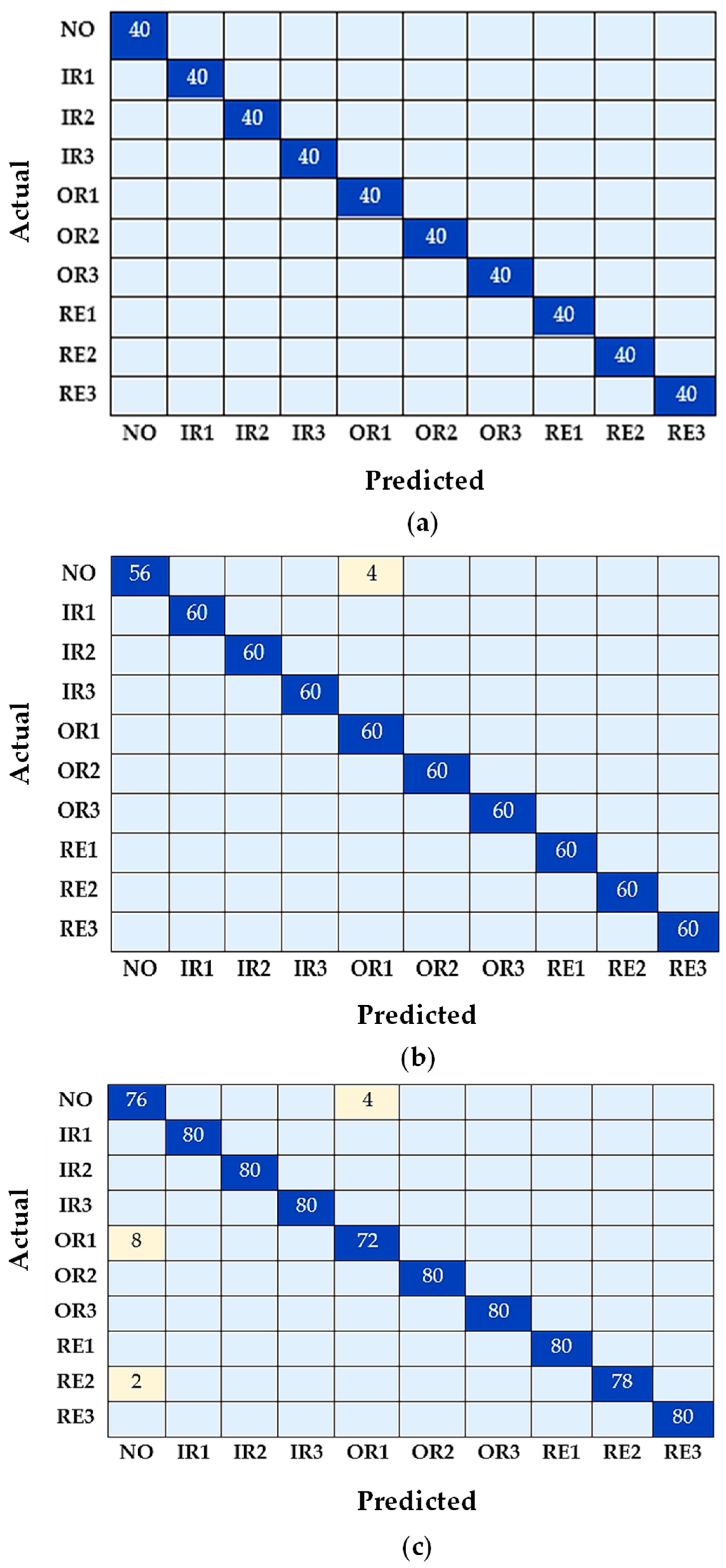
3.2.1. Experimental Results

To implement our proposed technique on the bearing dataset for the second case study, first, we applied the procedure of the CNN-based features to extract features from the collected vibration signals. The CNN feature extractor, as mentioned earlier, was employed for this purpose. Then, the extracted features are fed into the transformer for temporal relationship modelling. As previously mentioned, our algorithm incorporates several transformer encoder layers, employing self-attention mechanisms to capture long-range temporal dependencies within the extracted features. Additionally, there is a self-attention layer dedicated to linking the target and source inputs. The model uses layer normalisation and dropout regularisation to improve its ability to generalise to new data. It also uses a feed-forward network with linear layers and activation functions to process the features. The last linear layer maps the hidden representations to the number of output classes, and a Softmax layer generates probabilities for each class. The model makes predictions for input samples by considering their temporal relationships and the extracted features. Table 9 presents the overall testing classification accuracy, precision, recall, F-score, and their corresponding standard deviations for bearing faults using the second case study vibration dataset.
As can be seen from the data in Table 9, the classification model for bearing faults achieved a high performance with different training sizes. With the training size of 60%, the model achieved an overall accuracy of 99.18%, with high precision, recall, and F1-Score values of 99.14%, 99.18%, and 98.98%, respectively. As the training size increased to 70%, the model’s performance improved significantly, reaching near-perfect accuracy, precision, recall, and F1-Score scores of 99.96%. Finally, with the 80% training size, the model achieved perfect scores across all performance metrics, demonstrating high classification accuracy, precision, recall, and F1-Score values of 100%. These findings demonstrate the effectiveness and robustness of the classification model in accurately identifying bearing faults, with performance improving as the training size increases.
In Figure 12, we present a sample confusion matrix that showcases the classification outcomes derived from testing the model using 20%, 30%, and 40% of the accessible data. The confusion matrices in Figure 12 show that the model achieved a high rate of correct classifications across the testing datasets. However, there were some misclassifications, particularly involving the NO, OR1, and RE2 classes. The model misclassified four NO instances as OR1, eight OR1 instances as NO, and two RE2 instances as NO. Taken together, the confusion matrices reveal that the model achieves a high level of accuracy with the tested datasets, but encounters difficulties when classifying NO, OR1 and RE2.

3.2.2. Comparisons of Results

In this subsection, we perform a comparative analysis of different approaches using the same vibration dataset for the rolling bearings, which is specifically detailed in Table 10. Firstly, in reference [5], a CS-DNN technique is employed, which combines a deep neural network (DNN) method with two hidden layers and a Haar wavelet-based CS technique to classify rolling bearings from the same dataset, employing α = 0.1. Furthermore, ref. [51] presents classification results for bearing fault classifications using two distinct methods on the same dataset. The first method is based on a deep neural network (DNN), while the second method utilises a backpropagation neural network (BPNN). Additionally, in reference [52], classification results utilising a generic multi-layer perception (MLP) method are reported, using the same dataset in the second case study. From the results presented in the table, it is evident that our proposed method shows exceptional performance compared to the other methods. The approach referenced in [5], which utilises CS-DNN with α = 0.1, achieves a remarkable testing accuracy of 100%. In contrast, the methods [51] and [52] using DNN and BPNN, and MLP, respectively, demonstrate lower testing accuracies of 99.74% and 69.82% for [51], and 99.4% for [52]. However, our proposed method surpasses all others, achieving the highest average accuracy of 100% when tested with the 20% testing data subset. Moreover, even when tested with the larger 40% testing data subset, our proposed method still achieves a high accuracy of 99.43%. These findings highlight the superior performance of our proposed method, outperforming or matching the accuracy of other approaches on the given vibration dataset.

4. Conclusions

This study proposes a novel deep-learning architecture called the convolutional-transformer model with long-range temporal dependencies for bearing fault diagnosis using vibration signals. The model combines the strengths of convolutional neural networks (CNNs) and the transformer model to diagnose effectively faults in rotating machinery. The proposed method follows a sequential approach where CNNs are used for feature extraction from the vibration signals, and the transformer model is utilised to model the temporal relationships. By incorporating both local and long-range temporal dependencies, the proposed method achieves accurate fault diagnoses. The experimental results from two case studies demonstrate the effectiveness of the proposed model. In the first case study, using a bearing vibration dataset with six health conditions, the model achieves high classification accuracy, precision, recall, F1-score, and specificity, with low standard deviations. Similarly, in the second case study using a motor-bearing vibration dataset with ten health conditions, the model achieves excellent performance across all evaluation metrics. Taken together, the convolutional-transformer model proves to be an efficient and promising approach for bearing fault diagnosis, using the advantages of CNNs for local feature extraction and the transformer model for capturing long-range temporal dependencies. Further research in this area can explore its application in other domains and expand its potential for intelligent fault diagnosis.

Author Contributions

H.O.A.A. and A.K.N. conceived and designed this paper. H.O.A.A. performed the experiments. H.O.A.A. and A.K.N. wrote a draft of the manuscript and contributed to discussing the results in the manuscript. All authors have read and agreed to the published version of the manuscript.

Funding

This research received no external funding.

Data Availability Statement

The data presented in the first case study may be available on request from the first author, Hosameldin O. A. Ahmed.

Acknowledgments

Authors wish to thank Brunel University in London for their support.

Conflicts of Interest

The authors declare no conflict of interest.

References

  1. Ahmed, H.O.A.; Nandi, A.K. Condition Monitoring with Vibration Signals: Compressive Sampling and Learning Algorithms for Rotating Machines; John Wiley & Sons: Hoboken, NJ, USA, 2020. [Google Scholar]
  2. Wang, L.; Chu, J.; Wu, J. Selection of optimum maintenance strategies based on a fuzzy analytic hierarchy process. Int. J. Prod. Econ. 2007, 107, 151–163. [Google Scholar] [CrossRef]
  3. Higgs, P.A.; Parkin, R.; Jackson, M.; Al-Habaibeh, A.; Zorriassatine, F.; Coy, J. A survey on condition monitoring systems in industry. In Proceedings of the ASME 7th Biennial Conference on Engineering Systems Design and Analysis, Manchester, UK, 19–22 July 2004; Volume 41758, pp. 163–178. [Google Scholar] [CrossRef] [Green Version]
  4. Kim, J.; Ahn, Y.; Yeo, H. A comparative study of time-based maintenance and condition-based maintenance for optimal choice of maintenance policy. Struct. Infrastruct. Eng. 2016, 12, 1525–1536. [Google Scholar] [CrossRef]
  5. Ahmed, H.; Wong, M.; Nandi, A. Intelligent condition monitoring method for bearing faults from highly compressed measurements using sparse over-complete features. Mech. Syst. Signal Process. 2018, 99, 459–477. [Google Scholar] [CrossRef]
  6. Ahmed, H.O.A.; Nandi, A.K. Intrinsic Dimension Estimation-Based Feature Selection and Multinomial Logistic Regression for Classification of Bearing Faults Using Compressively Sampled Vibration Signals. Entropy 2022, 24, 511. [Google Scholar] [CrossRef]
  7. Tahir, M.M.; Khan, A.Q.; Iqbal, N.; Hussain, A.; Badshah, S. Enhancing Fault Classification Accuracy of Ball Bearing Using Central Tendency Based Time Domain Features. IEEE Access 2016, 5, 72–83. [Google Scholar] [CrossRef]
  8. Nayana, B.R.; Geethanjali, P. Analysis of Statistical Time-Domain Features Effectiveness in Identification of Bearing Faults From Vibration Signal. IEEE Sens. J. 2017, 17, 5618–5625. [Google Scholar] [CrossRef]
  9. Rauber, T.W.; Boldt, F.D.A.; Varejao, F.M. Heterogeneous Feature Models and Feature Selection Applied to Bearing Fault Diagnosis. IEEE Trans. Ind. Electron. 2014, 62, 637–646. [Google Scholar] [CrossRef]
  10. Prieto, M.D.; Cirrincione, G.; Espinosa, A.G.; Ortega, J.A.; Henao, H. Bearing Fault Detection by a Novel Condition-Monitoring Scheme Based on Statistical-Time Features and Neural Networks. IEEE Trans. Ind. Electron. 2012, 60, 3398–3407. [Google Scholar] [CrossRef]
  11. Guo, H.; Jack, L.; Nandi, A. Feature Generation Using Genetic Programming with Application to Fault Classification. IEEE Trans. Syst. Man Cybern. Part B (Cybern.) 2005, 35, 89–99. [Google Scholar] [CrossRef]
  12. Ayaz, E. Autoregressive modeling approach of vibration data for bearing fault diagnosis in electric motors. J. Vibroeng. 2014, 16, 2130–2138. [Google Scholar]
  13. Lin, H.-C.; Ye, Y.-C. Reviews of bearing vibration measurement using fast Fourier transform and enhanced fast Fourier transform algorithms. Adv. Mech. Eng. 2019, 11, 1687814018816751. [Google Scholar] [CrossRef]
  14. Tian, J.; Morillo, C.; Azarian, M.H.; Pecht, M. Motor Bearing Fault Detection Using Spectral Kurtosis-Based Feature Extraction Coupled With K-Nearest Neighbor Distance Analysis. IEEE Trans. Ind. Electron. 2015, 63, 1793–1803. [Google Scholar] [CrossRef]
  15. Farokhzad, S. Vibration based fault detection of centrifugal pump by fast fourier transform and adaptive neuro-fuzzy inference system. J. Mech. Eng. Technol. 2013, 1, 82–87. [Google Scholar] [CrossRef]
  16. Zhang, C.; Mousavi, A.A.; Masri, S.F.; Gholipour, G.; Yan, K.; Li, X. Vibration feature extraction using signal processing techniques for structural health monitoring: A review. Mech. Syst. Signal Process. 2022, 177, 109175. [Google Scholar] [CrossRef]
  17. Feng, Z.; Liang, M.; Chu, F. Recent advances in time–frequency analysis methods for machinery fault diagnosis: A review with application examples. Mech. Syst. Signal Process. 2013, 38, 165–205. [Google Scholar] [CrossRef]
  18. Wang, L.; Liu, Z.; Miao, Q.; Zhang, X. Time–frequency analysis based on ensemble local mean decomposition and fast kurtogram for rotating machinery fault diagnosis. Mech. Syst. Signal Process. 2018, 103, 60–75. [Google Scholar] [CrossRef]
  19. Yu, J.; Lv, J. Weak Fault Feature Extraction of Rolling Bearings Using Local Mean Decomposition-Based Multilayer Hybrid Denoising. IEEE Trans. Instrum. Meas. 2017, 66, 3148–3159. [Google Scholar] [CrossRef]
  20. Staszewski, W.; Worden, K.; Tomlinson, G. Time–frequency analysis in gearbox fault detection using the wigner–ville distribution and pattern recognition. Mech. Syst. Signal Process. 1997, 11, 673–692. [Google Scholar] [CrossRef]
  21. He, Q.; Wang, X.; Zhou, Q. Vibration Sensor Data Denoising Using a Time-Frequency Manifold for Machinery Fault Diagnosis. Sensors 2013, 14, 382–402. [Google Scholar] [CrossRef] [Green Version]
  22. Wen, L.; Li, X.; Gao, L.; Zhang, Y. A New Convolutional Neural Network-Based Data-Driven Fault Diagnosis Method. IEEE Trans. Ind. Electron. 2017, 65, 5990–5998. [Google Scholar] [CrossRef]
  23. Janssens, O.; Slavkovikj, V.; Vervisch, B.; Stockman, K.; Loccufier, M.; Verstockt, S.; Van de Walle, R.; Van Hoecke, S. Convolutional Neural Network Based Fault Detection for Rotating Machinery. J. Sound Vib. 2016, 377, 331–345. [Google Scholar] [CrossRef]
  24. Jiao, J.; Zhao, M.; Lin, J.; Liang, K. A comprehensive review on convolutional neural network in machine fault diagnosis. Neurocomputing 2020, 417, 36–63. [Google Scholar] [CrossRef]
  25. Chen, Z.; Deng, S.; Chen, X.; Li, C.; Sánchez, R.V.; Qin, H. Deep neural networks-based rolling bearing fault diagnosis. Microelectron. Reliab. 2017, 75, 327–333. [Google Scholar] [CrossRef]
  26. Qiao, M.; Yan, S.; Tang, X.; Xu, C. Deep Convolutional and LSTM Recurrent Neural Networks for Rolling Bearing Fault Diagnosis Under Strong Noises and Variable Loads. IEEE Access 2020, 8, 66257–66269. [Google Scholar] [CrossRef]
  27. Ahmed, H.O.A.; Nandi, A.K. Connected Components-based Colour Image Representations of Vibrations for a Two-stage Fault Diagnosis of Roller Bearings Using Convolutional Neural Networks. Chin. J. Mech. Eng. 2021, 34, 37. [Google Scholar] [CrossRef]
  28. Zhu, J.; Jiang, Q.; Shen, Y.; Qian, C.; Xu, F.; Zhu, Q. Application of recurrent neural network to mechanical fault diagnosis: A review. J. Mech. Sci. Technol. 2022, 36, 527–542. [Google Scholar] [CrossRef]
  29. Yang, Z.; Xu, B.; Luo, W.; Chen, F. Autoencoder-based representation learning and its application in intelligent fault diagnosis: A review. Measurement 2022, 189, 110460. [Google Scholar] [CrossRef]
  30. Neupane, D.; Seok, J. Bearing Fault Detection and Diagnosis Using Case Western Reserve University Dataset With Deep Learning Approaches: A Review. IEEE Access 2020, 8, 93155–93178. [Google Scholar] [CrossRef]
  31. Bhuiyan, R.; Uddin, J. Deep Transfer Learning Models for Industrial Fault Diagnosis Using Vibration and Acoustic Sensors Data: A Review. Vibration 2023, 6, 218–238. [Google Scholar] [CrossRef]
  32. Ahmed, H.O.A.; Nandi, A.K. Vibration Image Representations for Fault Diagnosis of Rotating Machines: A Review. Machines 2022, 10, 1113. [Google Scholar] [CrossRef]
  33. Lv, H.; Chen, J.; Pan, T.; Zhang, T.; Feng, Y.; Liu, S. Attention mechanism in intelligent fault diagnosis of machinery: A review of technique and application. Measurement 2022, 199, 111594. [Google Scholar] [CrossRef]
  34. Li, X.; Zhang, W.; Ding, Q. Understanding and improving deep learning-based rolling bearing fault diagnosis with attention mechanism. Signal Process. 2019, 161, 136–154. [Google Scholar] [CrossRef]
  35. Xu, Z.; Li, C.; Yang, Y. Fault diagnosis of rolling bearings using an Improved Multi-Scale Convolutional Neural Network with Feature Attention mechanism. ISA Trans. 2021, 110, 379–393. [Google Scholar] [CrossRef] [PubMed]
  36. Yang, Z.-B.; Zhang, J.-P.; Zhao, Z.-B.; Zhai, Z.; Chen, X.-F. Interpreting network knowledge with attention mechanism for bearing fault diagnosis. Appl. Soft Comput. 2020, 97, 106829. [Google Scholar] [CrossRef]
  37. Li, X.; Wan, S.; Liu, S.; Zhang, Y.; Hong, J.; Wang, D. Bearing fault diagnosis method based on attention mechanism and multilayer fusion network. ISA Trans. 2022, 128, 550–564. [Google Scholar] [CrossRef]
  38. Zhang, X.; Cong, Y.; Yuan, Z.; Zhang, T.; Bai, X. Early Fault Detection Method of Rolling Bearing Based on MCNN and GRU Network with an Attention Mechanism. Shock. Vib. 2021, 2021, 6660243. [Google Scholar] [CrossRef]
  39. Wang, Y.; Liang, J.; Gu, X.; Ling, D.; Yu, H. Multi-scale attention mechanism residual neural network for fault diagnosis of rolling bearings. Proc. Inst. Mech. Eng. Part C J. Mech. Eng. Sci. 2022, 236, 10615–10629. [Google Scholar] [CrossRef]
  40. Hao, Y.; Wang, H.; Liu, Z.; Han, H. Multi-scale CNN based on attention mechanism for rolling bearing fault diagnosis. In Proceedings of the Asia-Pacific International Symposium on Advanced Reliability and Maintenance Modeling (APARM)-IEEE, Vancouver, BC, Canada, 20–23 August 2020; pp. 1–5. [Google Scholar] [CrossRef]
  41. Vaswani, A.; Shazeer, N.; Parmar, N.; Uszkoreit, J.; Jones, L.; Gomez, A.N.; Kaiser, Ł.; Polosukhin, I. Attention is all you need. Adv. Neural Inf. Process. Syst. 2017, 30, 1–11. [Google Scholar]
  42. Hou, Y.; Wang, J.; Chen, Z.; Ma, J.; Li, T. Diagnosisformer: An efficient rolling bearing fault diagnosis method based on improved Transformer. Eng. Appl. Artif. Intell. 2023, 124, 106507. [Google Scholar] [CrossRef]
  43. Hou, S.; Lian, A.; Chu, Y. Bearing fault diagnosis method using the joint feature extraction of Transformer and ResNet. Meas. Sci. Technol. 2023, 34, 075108. [Google Scholar] [CrossRef]
  44. Cen, J.; Yang, Z.; Wu, Y.; Hu, X.; Jiang, L.; Chen, H.; Si, W. A Mask Self-Supervised Learning-Based Transformer for Bearing Fault Diagnosis With Limited Labeled Samples. IEEE Sens. J. 2023, 23, 10359–10369. [Google Scholar] [CrossRef]
  45. Wu, H.; Triebe, M.J.; Sutherland, J.W. A transformer-based approach for novel fault detection and fault classification/diagnosis in manufacturing: A rotary system application. J. Manuf. Syst. 2023, 67, 439–452. [Google Scholar] [CrossRef]
  46. Lecun, Y.; Bottou, L.; Bengio, Y.; Haffner, P. Gradient-based learning applied to document recognition. Proc. IEEE 1998, 86, 2278–2324. [Google Scholar] [CrossRef]
  47. Ahmed, H.; Nandi, A.K. Compressive Sampling and Feature Ranking Framework for Bearing Fault Classification With Vibration Signals. IEEE Access 2018, 6, 44731–44746. [Google Scholar] [CrossRef]
  48. Seera, M.; Wong, M.D.; Nandi, A.K. Classification of ball bearing faults using a hybrid intelligent model. Appl. Soft Comput. 2017, 57, 427–435. [Google Scholar] [CrossRef]
  49. Wong, M.L.D.; Zhang, M.; Nandi, A.K. Effects of compressed sensing on classification of bearing faults with entropic features. In Proceedings of the 2015 IEEE 23rd European Signal Processing Conference (EUSIPCO), Nice, France, 31 August–4 September 2015. [Google Scholar] [CrossRef] [Green Version]
  50. Case Western Reserve University Bearing Data Center. Available online: https://engineering.case.edu/bearingdatacenter/download-data-file (accessed on 27 June 2023).
  51. Jia, F.; Lei, Y.; Lin, J.; Zhou, X.; Lu, N. Deep neural networks: A promising tool for fault characteristic mining and intelligent diagnosis of rotating machinery with massive data. Mech. Syst. Signal Process. 2016, 72, 303–315. [Google Scholar] [CrossRef]
  52. de Almeida, L.F.; Bizarria, J.W.; Bizarria, F.C.; Mathias, M.H. Condition-based monitoring system for rolling element bearing using a generic multi-layer perceptron. J. Vib. Control 2015, 21, 3456–3464. [Google Scholar] [CrossRef] [Green Version]
Figure 1. (a) A typical roller bearing; (b) Rolling element bearing geometry.
Machines 11 00746 g001
Figure 2. The architecture of the convolutional-transformer model with long-range temporal dependencies.
Machines 11 00746 g002
Figure 3. The architecture of the proposed CNN Feature Extractor.
Machines 11 00746 g003
Figure 4. The overall architecture of the transformer [41].
Machines 11 00746 g004
Figure 5. The schematic representation of multi-head attention.
Machines 11 00746 g005
Figure 6. The overall architecture of the temporal transformer encoder used in our proposed method.
Machines 11 00746 g006
Figure 7. Typical time series plots for the above-mentioned six conditions [5].
Machines 11 00746 g007
Figure 8. The test rig utilised to collect the vibration data of bearings of the first case study [7].
Machines 11 00746 g008
Figure 9. Confusion Matrix: classification results for the first case study vibration dataset with testing dataset, depicting (a) 20%, (b) 30%, and (c) 60%.
Machines 11 00746 g009
Figure 10. Feature visualisation in three feature spaces (a) original data features, (b) CNN feature extraction based features, and (c) convolutional-transformer based features (our proposed method).
Machines 11 00746 g010
Figure 11. The test rig used to collect the CWRU vibration data of bearings [50].
Machines 11 00746 g011
Figure 12. Confusion Matrix: classification results for the second case study vibration dataset with testing dataset, depicting (a) 20%, (b) 30%, and (c) 60%.
Machines 11 00746 g012
Table 1. Description of bearing dataset.
Bearing Health
Condition
Number of
Samples
Number of
Data Points
NormalNO1606000
NW1606000
FaultIR1606000
OR1606000
RE1606000
CA1606000
Table 2. The selected set of parameters in the CNN feature extraction process of the proposed method.
ParameterValueDescription
Number of convolutional layers2The number of convolutional layers in the CNN feature extractor.
Number of filters per convolutional layer64,128The number of filters in each convolutional layer.
Kernel size3 × 3The size of the kernels used in the convolutional layers.
Stride1The stride used in the convolutional layers.
Padding 1The padding used in the convolutional layers.
Number of max pooling layers2The number of max pooling layers in the CNN feature extractor.
Kernel size2 × 2The size of the kernel used in the max pooling layers.
Stride2The stride used in the max pooling layers.
Fully connected layers256The size of the fully connected layers in the CNN feature extractor.
Activation functionReLUThe activation function used after each convolutional layer.
Reduced dimensionalityThe factor by which the dimensionality of the output from the convolutional layers is reduced by the max pooling layer.
Table 3. The selected set of parameters in the temporal transformer encoder part of the proposed method.
ParameterValueDescription
Hidden size128The size of the hidden layer.
Number of layers6The number of transformer encoder layers.
Number of heads8The number of heads in the multi-head attention layers.
Number of classes6The number of the output classes in the bearing data of the first case study.
Activation functionReLUThe activation function used after the linear layers.
Table 4. The training options and evaluation metrics utilised for assessing the performance of the classification models.
Training OptionValue
Loss functionCross Entropy Loss
OptimizerAdam
Learning rate0.0001
Number of epochs300
Evaluation metricsClassification accuracy, precision, recall, F1-score, and specificity
Table 5. A description of the evaluation metrics used for assessing the performance of the classification models.
MetricDefinitionFormula
AccuracyThe proportion of instances that were correctly classified by the model. A c c u r a c y = ( T P + T N ) / ( T P + T N + F P + F N )
PrecisionThe proportion of instances that were classified as positive that were positive.Precision = TP/(TP + FP)
RecallThe proportion of positive instances that were correctly classified by the model.Recall = TP/(TP + FN)
F1 scoreA weighted average of the precision and recall metrics.F1 score = 2 ∗ (precision ∗ recall)/(precision + recall)
SpecificityThe proportion of negative instances that were correctly classified by the model.Specificity = TN/(TN + FP)
Table 6. The overall testing classification accuracy, precision, recall, F-score results, and their corresponding standard deviations for bearing faults using the first case study vibration dataset.
Training SizeAccuracy
(%)
Precision
(%)
Recall
(%)
F1-Score
(%)
Specificity
(%)
Std. Dev
60%99.4399.4199.4399.431000.5
70%99.8799.8599.8799.871000.1
80%1001001001001000.0
Table 7. Comparison of classification results from the literature on vibration bearing dataset in the first case study.
Ref.MethodTesting Accuracy (%)
[11]Genetic programming—based features (unnormalised data)
ANN96.5
SVM97.1
[47]CS-FS99.7
CS-LS99.5
CS-Relief99.8
CS-PCC99.8
CS-Chi-299.5
[48](FMM-RF)
SampEn99.7
PS99.7
SampEn + PS99.8
[49]SVM Classifier with:
Entropic features98.9
Compressive sampling followed by signal recovery:
α = 0.5 92.4
α = 0.25 84.6
Our proposed method
Highest average accuracy (with 20% testing data)100
Lowest average accuracy (with 40% testing data)99.43
Table 8. Description of bearing health conditions in the vibration dataset used for the second case study.
Health ConditionFault Width (mm)Classification Label
NO01
RE10.182
RE20.363
RE30.534
IR10.185
IR20.366
IR30.537
OR10.188
OR20.369
OR30.5310
Table 9. The overall testing classification accuracy, precision, recall, F-score results, and their corresponding standard deviations for bearing faults using the second case study vibration dataset.
Training SizeAccuracyPrecisionRecallF1-ScoreSpecificityStd. Dev
60%99.1899.1499.1898.981000.6
70%99.9699.9799.9699.9699.590.02
80%1001001001001000.0
Table 10. Comparison of classification results from the literature on vibration bearing dataset in the second case study.
Ref.MethodTesting Accuracy (%)
[5] CS - DNN   with   α = 0.1 100
[51]DNN99.74
BPNN69.82
[52]MLP99.4
Our proposed method
Highest average accuracy (with 20% testing data)100
Lowest average accuracy (with 40% testing data)99.43
Disclaimer/Publisher’s Note: The statements, opinions and data contained in all publications are solely those of the individual author(s) and contributor(s) and not of MDPI and/or the editor(s). MDPI and/or the editor(s) disclaim responsibility for any injury to people or property resulting from any ideas, methods, instructions or products referred to in the content.

