Tires and Vehicle Lateral Dynamic Performance: A Corrective Algorithm for the Influence of Temperature

Abstract

The automotive industry is experiencing increasing competition, and vehicle development is becoming increasingly complex. Manufacturers must therefore be able to rapidly compare the outcomes of experimental tests carried out under different conditions. Robust simulation tools that can adjust for external factors have the potential to save a significant amount of time. In this regard, the purpose of this paper is to propose a method for evaluating the effect of asphalt temperature on tire and vehicle lateral dynamic performance, based on empirical data. Because rubber is a viscoelastic material, its properties are heavily influenced by the operating conditions. Therefore, a corrective algorithm must be created to enable the transfer of results obtained from tests carried out under different asphalt temperature conditions to a reference temperature of 25 °C. This article presents an analytical model that accurately describes this phenomenon, as well as the methods employed to generalize and optimize the model. Generalizability represents a crucial aspect of this research, as the model must be widely applicable across several vehicle categories while requiring minimal data to perform the corrections effectively. Finally, the analytical compensatory tool was incorporated into a MATLAB bicycle model to update the numerical transfer function measurements that describe the vehicle’s dynamic behavior during experimental maneuvers. These results indicate that modest data is needed to achieve good levels of accuracy, making the model and vehicle dynamics implementation promising.

1. Introduction

Modern vehicles are characterized by the ever-growing presence of sensors [1,2], active systems [3,4,5,6], assisted and autonomous driving [7,8,9] and intelligent control units [10,11]. These kinds of innovative technologies have one thing in common: all of them need reliable and complex physical data to build up internal models of the vehicle they aim to act upon.

It is well established in the automotive engineering sector that one of the most important components to be described in a vehicle is the tire. The forces and moments necessary to accelerate, brake and handle an automobile pass through this component; therefore, an accurate model of tire behavior is key to achieve a reasonably precise vehicle dynamics model. From the widespread magic formula of Pacejka [12] or simpler models, such as the Brush Model [13], to the most recent integrated methodologies [14,15,16], the study of tire dynamics is a fertile source of research and advancements. Most of the results are based on the detailed modelling of material mechanics or direct experimental extrapolation.

The Stellantis Balocco Proving Ground [17] is one of the largest testing centers in the world, where some 200,000 h of tests are conducted every year. In this context, while studying the outcomes of the experimental maneuvers performed and the data acquired, it was noted that certain vehicle parameters assume very different values if the asphalt temperature changes. The most affected of the vehicle parameters seems to be the cornering stiffness of the front and rear tires.

Since this parameter is fundamental to inspect the vehicle’s lateral dynamic behavior, it is necessary to develop an analytical model to describe the phenomenon and compensate the temperature variation effect—this is the main goal of this article.

Without this kind of compensative model, it might not be possible to effectively compare the results of tests performed, for instance, on different days resulting in a waste of time and resources. After a short review of some basic concepts about the tire and its properties, the problem previously defined will be studied in detail. The goal of this paper is the application of an established temperature dependence model to a set of experimental tests during full-vehicle maneuvers, in order to correct the observed behavior by adjusting the lateral dynamics response. The results come from a test campaign of seven vehicle models with similar overall characteristics (B-Segment Hybrid Subcompact Crossover SUVs), while one of them is chosen as the case study for which the specific results are presented. The methodology proposed should, however, be applicable to other vehicle categories, which shall be explored in future publications. This article represents the first step towards a comprehensive compensatory model and experimental methodology.

The tire is the only part of the car that touches the road. Tires must strike a balance between traction, comfort, durability, energy efficiency and overall cost. As a result of these competing needs, tires are very complex to design and build [18,19]. The rubber, natural or synthetic, is one of the most important constituents of a tire. Rubber is part of the elastomers plastics family [20]. Being a viscoelastic material, rubber’s properties are very sensitive to the external conditions. Elastomers do not obey Hooke’s law perfectly, but for a given excitation amplitude, frequency and temperature, the relationship between stress and strain can be understood through the following equation [21,22]:

$$\sigma =E*·\epsilon =\left(E^{\prime }+i{E}^{″}\right)\epsilon$$

(1)

where $E*$ is the elastic modulus (in complex form) that defines the phase and gain between stress and strain, and $i$ is the imaginary unit. $E*$ is formed by two parts: the loss modulus, $E″$ (stress-related dissipation proportional to the strain rate), and the storage modulus, $E^{\prime }$ (stress-related dissipation proportional to the strain itself). By calculating the ratio between the two factors, it is possible to define the dissipation factor, $\tan \delta$, that describes the ratio between the elastic and viscous responses of a generic compound of rubber. As proposed by [22] and reported in Figure 1, the complex elastic modulus varies with temperature and frequency.

A monotonic decrease is observed in both the storage and loss moduli as the temperature increases, with the most notable gradient occurring at low values. Additionally, there is a peak in the dissipation factor at a certain temperature, which shifts towards a higher temperature with an increase in excitation frequency. Due to tire operating conditions, the temperature and excitation frequency play crucial roles in determining the complex elastic modulus.

The generation of cornering forces [23,24] is directly linked to the compliance of the tire that allows the tread to move relative to the center of the wheel and with the same velocity on the ground. Consequently, localized sliding between the tire and road occurs, and for this reason the shape of the contact zone is distorted. Any increase in the sideslip angle, $\alpha$, leads to an enhanced stretching resulting in a wider slip zone. For low values of the sideslip angle, the side (or cornering) force increases linearly with $\alpha$. The slope $\partial F_{cornering}/\partial \alpha$ of the curve in the origin is defined as the cornering stiffness and written as $C_{\alpha }$:

$$C_{\alpha }={\left(\frac{\partial F_{cornering}}{\partial \alpha }\right)}_{\alpha =0}$$

(2)

Since the cornering stiffness is usually expressed as a positive number while in the initial part of the curve, $F_{cornering}\left(\alpha \right)$, the derivative $\partial F_{cornering}/\partial \alpha$ is always expressed as a negative number. The cornering force, $F_{cornering}$, can be expressed for low values of the sideslip angle ($\left|\alpha \right|<4°$), such as:

$$F_{cornering}=-C_{\alpha }\alpha$$

(3)

This expression is quite useful for studying the dynamic behavior of vehicles under the assumption of small sideslip angles, as it actually occurs in normal driving conditions. This expression is essential in the study of the stability of linearized models. The ratio between the cornering stiffness and the normal force is usually referred to as the cornering stiffness coefficient.

There are at least three different temperatures that may be considered important factors controlling the thermal conditions of a rolling tire [25]. The most common measure of such thermal conditions is the ambient air temperature, while the other two are the pavement temperature and tire temperature. The latter is the most difficult to establish, as the temperatures of different parts of rolling tires differ considerably. For this reason, obtaining representative values is problematic. Moreover, tire temperature is dependent on many factors, such as internal energy losses, cooling effects caused by airflows, solar radiation, road temperature and cooling effects caused by snow or water on the pavement. However, road temperature is mainly determined by air temperature, solar radiation, wind and precipitation. It may also be influenced by rolling tires. Moreover, road temperature influences tire temperature considerably.

In their study [26], Dang Lu et al. performed some handling tests in order to obtain the cornering properties of a reference tire for a small range of steering angles in six different temperature conditions. From the test results, it was observed that the lateral force value changed depending on the temperature: the reason for this can be easily understood given that, as they demonstrated, the cornering stiffness of the tire gradually decreased with the increase of the temperature under the same vertical load.

In order to consider the cornering stiffness dependence on temperature, R. Okubo and K. Oyama developed an empirical relation [27,28] based on the measurements that they made. This relation was introduced in a simple bicycle model to study the changes of the vehicle’s response at different operating temperatures. It is expressed as:

$$\frac{C_{\alpha }}{F_z}=\frac{p_1}{t_{tb}-p_2}+p_3$$

(4)

where $C_{\alpha }$ is the cornering stiffness of the tire, $F_z$ is the vertical load, $t_{tb}$ is the tread bulk temperature and $p_1$, $p_2$, $p_3$ are three coefficients that must be statistically computed using the experimental data. Therefore, $C_{\alpha }$ will reduce monotonically in function of $t_{tb}$. This model will be applied in a completely new context. In fact, with experiments performed with a tire on test bench, we will verify whether this model can be extended to experimental maneuvers executed by different vehicles on the road.

Another way to consider the effect of temperature on the cornering stiffness is to consider the tire brush model [29]. This model consists of a row of elastic bristles that touch the road plane and can deflect in a direction parallel to the road surface. These bristles are called tread elements, and their compliance represents the elasticity of the combination of the carcass, belt and actual tread elements of the real tire. This model can be employed to determine simple first order physical relations between different tire properties [22]. Under the assumption that the treads are the only elements subjected to deformation (infinitely stiff carcass), the cornering stiffness, $C_{\alpha }$, can be defined as:

$$C_{\alpha }=2c_{py}{a}_c^2$$

(5)

where $c_{py}$ is the tread shear stiffness per unit length in a lateral direction, $a_c$ is half of the contact patch length.

As in Equation (6), $c_{py}$ can be written as:

$$c_{py}=\frac{c_A}{2b_c}$$

(6)

where $c_A$ is the shear stiffness of the treads and $b_c$ is half of the contact patch width. From Figure 2 and Equation (7), it is possible to derive the shear stiffness of one tread element of infinitesimal area, $d{c}_A$, as shown by [22]:

$$d{c}_A=G*\frac{dA}{h_t}=\frac{E*}{2\left(1+\upsilon \right)}\frac{dA}{h_t}$$

(7)

where $F$ is the force that is acting on the tread element, $x$ is the transverse displacement, $G*$ is the complex shear modulus, $dA$ is the infinitesimal area of one tread element, $h_t$ is its height, $E*$ is the complex elastic modulus and $\upsilon$ is Poisson’s ratio.

But considering that

$$c_A={{\displaystyle \int }}_{A}d{c}_A=\frac{E*}{2\left(1+\upsilon \right)}\frac{A}{h_t}$$

(8)

and knowing that value of the contact patch area, $A$, is given by:

$$A=2a_c·2b_c$$

(9)

it is possible, substituting Equations (8) and (9) in Equation (6), to obtain the following expression for the tread shear stiffness per unit length in a lateral direction, $c_{py}$:

$$c_{py}=\frac{c_A}{2b_c}=\frac{E*}{2\left(1+\upsilon \right)}\frac{A}{h_t}\frac{1}{2b_c}=\frac{E*}{2\left(1+\upsilon \right)}\frac{2a_c}{h_t}=\frac{E*}{1+\upsilon }\frac{a_c}{h_t}$$

(10)

So, finally, substituting Equation (10) in Equation (5), the cornering stiffness, $C_{\alpha }$, can be redefined as:

$$C_{\alpha }=2\frac{E*}{1+\upsilon }\frac{a_c^3}{h_t}$$

(11)

The result is that the cornering stiffness is a function of the complex elastic modulus, $E*$, which is in turn a function of temperature and excitation frequency. Therefore, $C_{\alpha }$ will reduce monotonically in function of the temperature and with the tire rolling speed it must raise. A demonstration of the validity of these conclusions can be found in the graph shown in Figure 3, where the cornering stiffness and the storage modulus are plotted as a function of temperature.

The main goal of this paper is to study how temperature influences the tire and vehicle lateral dynamic performance. The aim is to achieve a temperature variation effect compensation in order to effectively rescale the numerical transfer functions of the vehicles considered. To reach the scope, it was necessary to build a wide database performing many experimental tests and to accomplish several objectives, namely:

• To identify an analytical model able to capture the phenomenon accurately;
• To generalize and optimize the model identified. It has to become a ready-to-use tool for a large number of vehicle categories requiring, for every correction that has to be done, the smallest amount of data possible;
• To validate the analytical compensative tool from a statistical point of view;
• To implement it in a MATLAB bicycle model to update the measured values of the numerical transfer functions that describe the dynamic behavior of the vehicle during the maneuvers and compare the results with the original curves.

2. Model Definition

2.1. Database Acquired and Maneuvers

In order to develop this project, 152 experimental tests were performed on seven different vehicles. Among them there were four B-segment passenger cars (one mini MPV and three subcompact crossover SUVs), a C-segment subcompact crossover SUV, a D-segment compact crossover SUV car and one light-duty commercial vehicle. The tests consisted in performing on the track one of the two ISO-normed maneuvers that will be described below using vehicles equipped with an instrumented steering wheel, a GPS unit, height sensors (or suspension travel sensors), an inertial measurement unit (IMU), a sideslip angle sensor and a control unit.

After each test, a text file containing the information collected was produced as output (Section 4). In these files it is possible to find the following data:

• All the parameters necessary to build a bicycle model that describe the vehicle and its dynamic behavior during the maneuver;
• A table indicating the numerical values assumed by a wide set of transfer functions in the frequency domain during the maneuver;
• Tables indicating the analytical values assumed by the same set of transfer functions mentioned at the previous point in the frequency domain during the maneuver. There are two different tables for two distinct approaches: in one case the relaxation length of the tires is considered, while in the other they are not.

Another fundamental piece of information that is acquired is the local instantaneous asphalt temperature. This is acquired by checking the reports of the sensors that are installed close to the road surface all around the testing center.

Two different types of ISO-normed maneuver were executed at different temperatures to gather the information needed to analyze the behavior of the vehicles [30,31].

The first one is the frequency sweep (upper graph in Figure 4). It consists of a series of steering and counter-steering actions performed at a constant vehicle speed with a progressively increasing frequency. The counter-steering movement starts when the target lateral acceleration value (0.3 g, 0.5 g or 0.7 g) is reached. The goal of this maneuver is to make the car perform a sort of “double lane change” iterated. The second type of maneuver considered is the slow input steering (lower graph in Figure 4). It is based on a slowly increasing steering wheel angle that is applied while the vehicle proceeds at constant speed. Once the target value (180° or sometimes 120°) has been reached, the steering wheel angle is maintained for a short interval (less than 10 s) and then the steering wheel is released. In this way the initial steady-state condition is recovered quickly. The vehicles that are tested describe a snail-like trajectory. For both the abovementioned maneuvers, the duration is in general comprised between 20 s and 40 s.

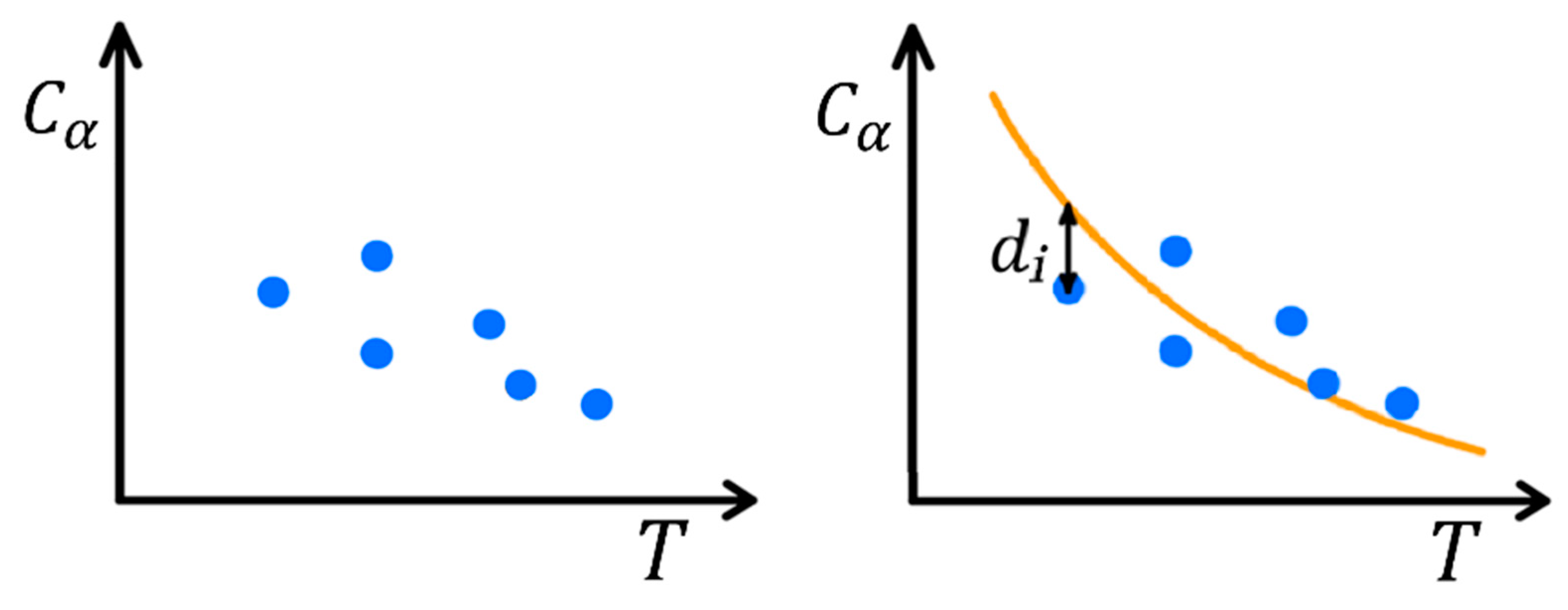
2.2. Cornering Stiffness Analytical Optimal Model

At this point, a slightly modified version of the Okubo and Oyama model can be introduced. It is based on the following relation:

$$C_{\alpha }=\frac{p_2}{t_{tb}-p_1}+p_3$$

(12)

where $C_{\alpha }$ is the cornering stiffness of the front or rear axle tires (note that the entire project is based on a bicycle model approach), $t_{tb}$ is the tread bulk temperature (in this case it will be substituted by the asphalt temperature, $T_a$) and $p_1$, $p_2$ and $p_3$ are three characteristic parameters of the model. Focusing on these parameters:

• From a mathematical point of view, $p_1$ is the temperature at which the cornering stiffness is equal to infinity. Physically, this is the so-called glass transition temperature, $T_g$;
• From a mathematical point of view, $p_3$ is the cornering stiffness when the temperature is equal to infinity. Physically, this is the decomposition temperature and, depending on the tire compound, it is close to 150 °C.

However, $p_1$ can be known a priori given the type of tires mounted on the tested vehicle. In fact, for each category (summer tires, winter tires) there is a different compound characterized by a typical range of $p_1$ ($T_g$) values. So, in accordance with [32,33,34,35], considering the fast evolution of research in the rubber field and considering the most common modern tire categories, the table shown below was built (

Table 1. Values of the $p_1$ coefficient for different modern tires categories.

Tires Category	Value of p1	Units
Summer Tires	−25	[°C]
Summer GT Tires	−20	[°C]
All Season Tires	−32	[°C]
Winter Tires	−40	[°C]

).

For every dataset that must be analyzed, the value of $p_1$ is chosen from Table 1 as a function of the tires equipped on the vehicle. Concerning $p_2$ and $p_3$, these two parameters are initially computed while solving a system of equations employing an optimization script on MATLAB.

2.3. MATLAB Optimization Script

From a theoretical point of view, the goal of the MATLAB optimization script is to compute $p_2$ and $p_3$ so that the sum of the distances, $d_i$, between the hyperbole of the Okubo and Oyama modified model (orange curve in Figure 5) and each of the points representing the experimental measurements (blue points in Figure 5) is minimized.

This theoretical idea can be transformed to a working tool in the following way: Having a dataset composed of $n$ measurements ($C_i-T_i$, where $i$ = 1, 2, 3, 4, …, $n$), the values of $p_2$ and $p_3$ can be obtained using the MATLAB function optimvar to solve this $n$-equations-2-unknowns-linear-system:

$$\{\begin{array}{c}\begin{array}{c}{C}_1=\frac{p_2}{T_1-p_1}+p_3\\ C_2=\frac{p_2}{T_2-p_1}+p_3\end{array}\\ \begin{array}{c}{C}_3=\frac{p_2}{T_3-p_1}+p_3\\ ⋮\end{array}\\ C_n=\frac{p_2}{T_n-p_1}+p_3\end{array}$$

(13)

The case considered is a frequency sweep maneuver (front axle measurements) performed with a lateral acceleration target of 0.5 g by a B-segment hybrid subcompact crossover SUV in a wide temperature range (5.5–52.8 °C). Additionally, Figure 5 shows the error percentage between the analytical model and each of the experimental measurements.

The analytical model works very well even if the temperature measured is not the tread bulk one (as originally done by Okubo and Oyama) but the asphalt one. This leads to an important advantage: equipping the tested vehicles with tire temperature sensors—a very time-consuming operation—is not necessary. Moreover, the output data produced by these sensors need to be post-processed before they can be studied, which requires a lot of time. Lastly, it is important to underline that in the values of the cornering stiffnesses measured, there is also a contribution from the suspension system. This explains why the values acquired for the front axle and the rear axle are generally slightly different, even if the tires mounted are exactly the same. The procedure described above was repeated for all the vehicles tested at every lateral acceleration level. For each dataset, the parameters of the analytical curves, $p_2$ and $p_3$, were computed (for both the maneuvers considered). In all these cases, the average error was between 1% and 2%.

3. Model Application

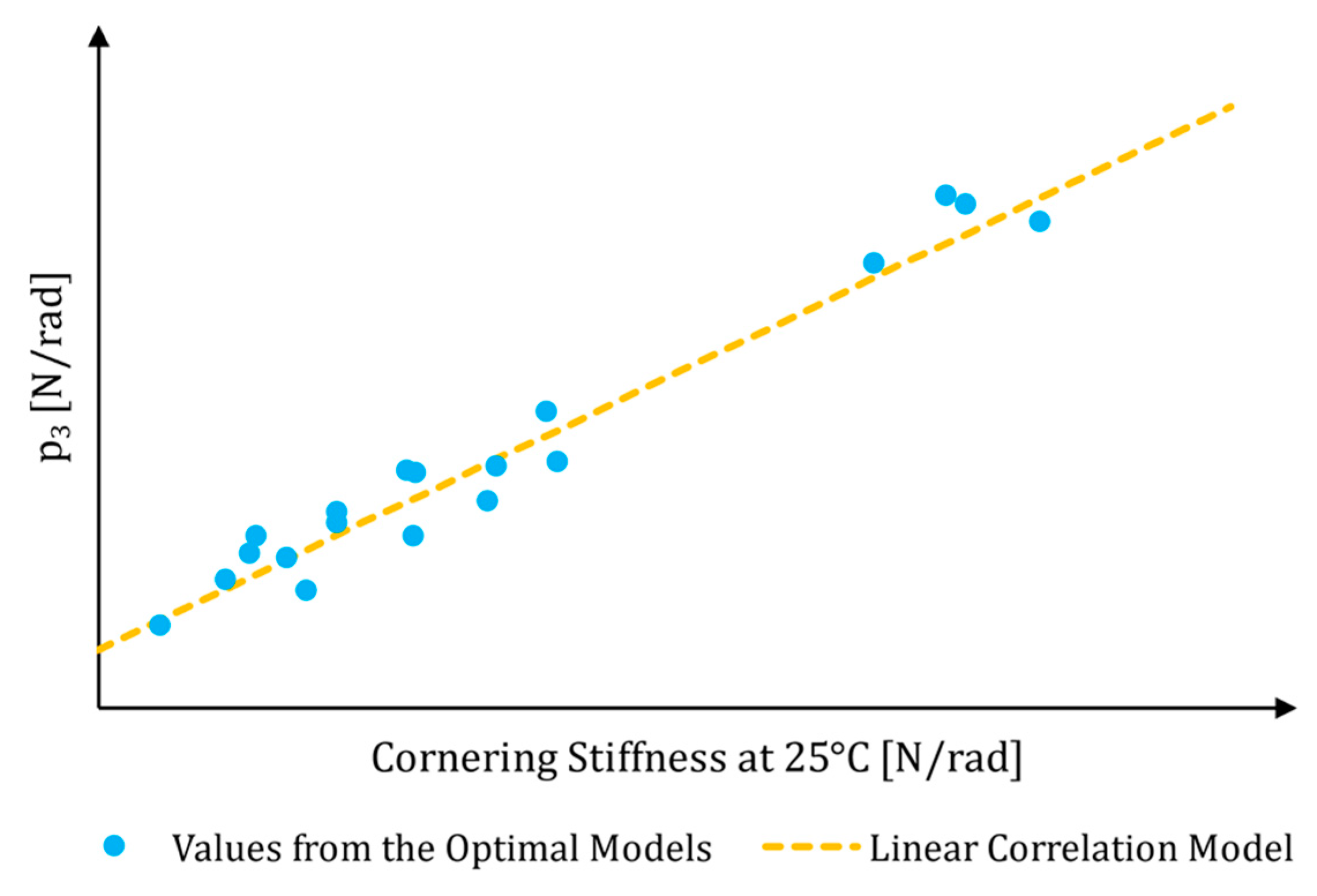
3.1. Linear Correlation Model

The step that will be discussed below is at the core of this work: It is necessary to define a mathematical relationship to link one of the two parameters of the Okubo and Oyama modified model, $p_2$ or $p_3$, and the cornering stiffness of the two axles at 25 °C (this temperature was set as the reference one for the corrections). The goal, in fact, is to find a way to compute all the previously mentioned variables in the case in which only one experimental measurement ($T_{mes}-C_{mes}$) is available as an input. This is necessary because during the development stages of a vehicle, time and resources are limited, and it is not possible to perform many tests (such limitations were not present in this project). To be clear, a situation like the one shown in the graphs at the end of the last section, in which eleven measurements were available, is not realistic and is not feasible. Thus, by studying the curves of the analytical models and the parameters calculated above, a correlation was identified between $p_3$ and $C_{25°\mathrm{C}}$, as shown in Figure 6.

In this graph, all the cases that were analyzed are plotted together: no distinction is made between front and rear axle and the maneuver performed. The light blue points coming from the analytical optimal models are distributed along a straight line that can be parameterized easily. The linear correlation, from a physical point of view, is consistent because the curves of the Okubo and Oyama model present an extremely non-linear section at low temperatures and an almost linear part at the higher ones (as it is possible to see from Figure 7). Once the angular coefficient, $m$, and the constant term, $q$, have been computed, the parameter $p_3$ can be expressed as a function of the cornering stiffness at 25 °C, $C_{25°\mathrm{C}}$, as in Equation (14):

$$p_3=m{C}_{25°\mathrm{C}}+q$$

(14)

At the same time, the other unknown parameter, $p_2$, can be defined by drawing upon Equation (12) and the unique experimental measurement available ($T_{mes}-C_{mes}$), through Equation (15):

$$p_2=(C_{mes}-p_3)\left(T_{mes}-p_1\right)$$

(15)

Finally, remembering that the value of $p_1$ is known and combining Equation (12) with Equation (15), $p_3$ and $C_{25°\mathrm{C}}$ can be derived, thus solving the 2-equations-2-unknows-linear system in Equation (16)

$$\{\begin{array}{c}{p}_3=m{C}_{25°\mathrm{C}}+q\\ C_{25°\mathrm{C}}=\frac{(C_{mes}-p_3)\left(T_{mes}-p_1\right) }{25°\mathrm{C}-p_1}+p_3\end{array}$$

(16)

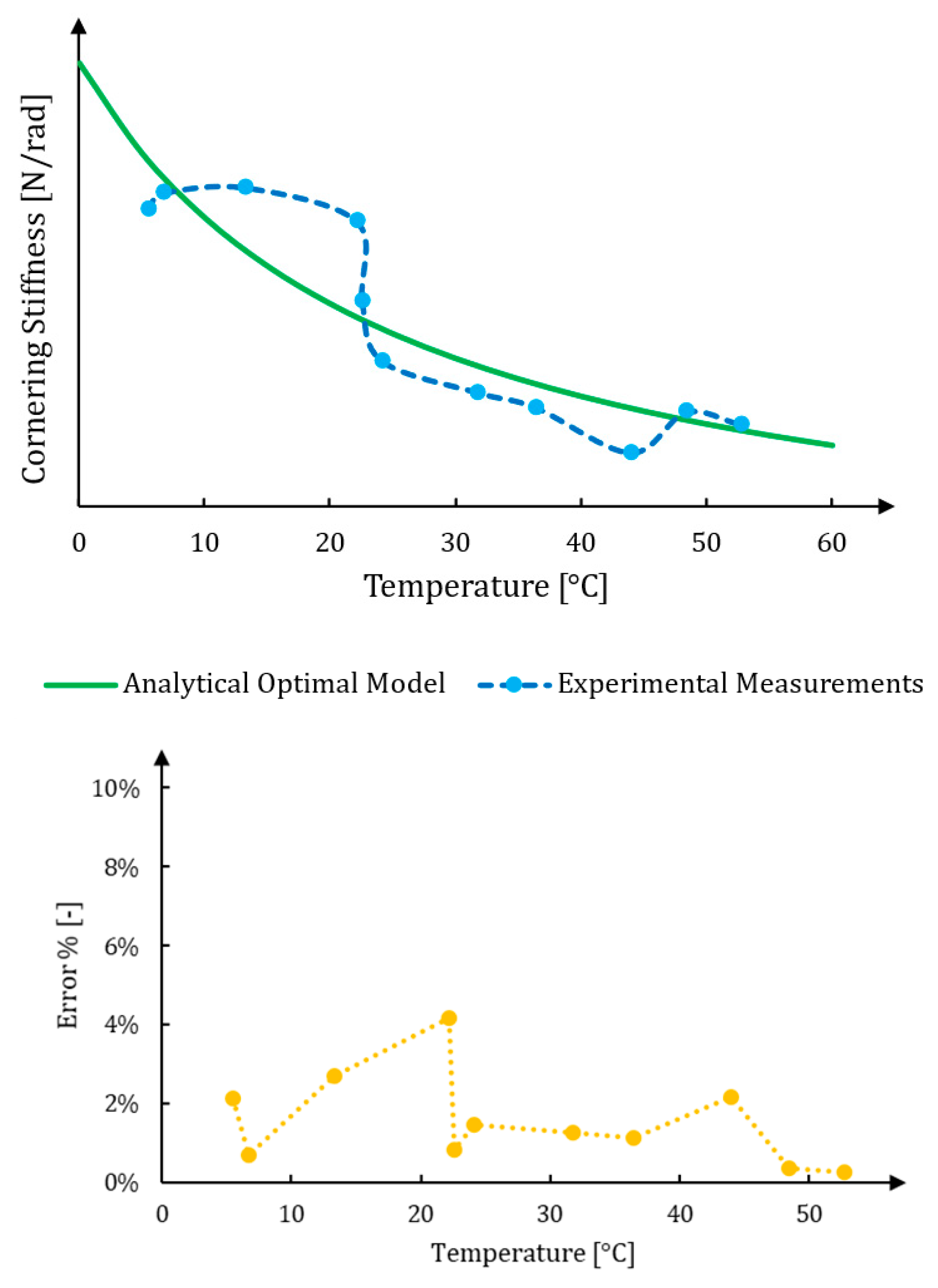
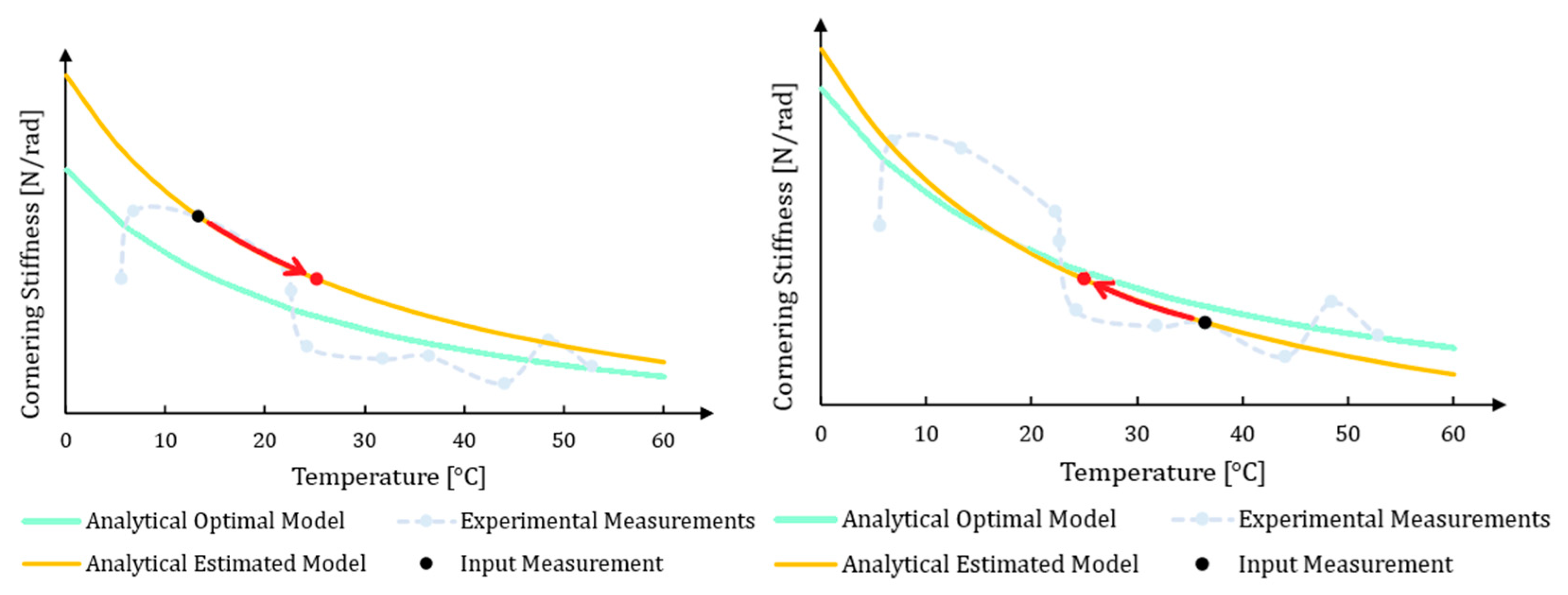
3.2. Analysis of the New Results

Now, some of the new results obtained can be discussed. Two distinct examples are considered. The case chosen as reference for both of them is again a frequency sweep maneuver (front axle measurements) but this time performed with a lateral acceleration target of 0.3 g by a B-segment hybrid subcompact crossover SUV in a wide temperature range (5.5–52.8 °C).

Evidently, it is possible to calculate the cornering stiffness at 25 °C using only one experimental measurement and without losing too much accuracy. Changing the input measurement can cause the results to vary slightly. In fact, considering the graphs of Figure 8, choosing as an input the third measurement available (upper plot) causes the cornering stiffness at 25 °C to be slightly overestimated with respect to the one computed with the analytical optimal model. Instead, choosing as an input the eighth measurement available (lower plot) causes the cornering stiffness at 25 °C to be almost equal to the one computed with the analytical optimal model.

Employing the above-described method to correct the cornering stiffness at the reference temperature of 25 °C, a couple of Gaussian curves were calculated for each maneuver performed by every vehicle. The first one represents the dispersion of the experimental measurements, while the second one represents the dispersion of the results once the correction has been applied (and thus the temperature effect has been compensated). Consequently, most of the remaining dispersion is due to other external factors. Comparing the two normal distributions, it is possible to understand how much of the original dispersion can be removed.

The graph in Figure 9 shows the overall situation of the B-segment hybrid subcompact crossover SUV, which is the reference vehicle of this paper. The curves have been realized by plotting two normal distributions with a mean value equal to zero and standard deviation equal to the average of the standard deviations computed previously. The unit of measure of the main horizontal axis is the averaged standard deviation of the experimental measurements, ${\sigma }_1$, while the unit of measure of the secondary horizontal axis is the averaged standard deviation of the measurements corrected in temperature, ${\sigma }_2$. Considering that temperature variation is a seasonal phenomenon, curve #1 can be defined as the dispersion of a set of measurements acquired randomly in a period of time equal to one year. Curve #2 can be described, instead, as the dispersion of the same set of measurements after the oscillations have been compensated due to the temperature effect. It has to be underlined that, in this situation, adjusting the cornering stiffness values enabled the reduction of the standard deviation by 61%. In general, for the other vehicles and maneuvers studied, the decrease in $\sigma$ was between 55% and 65%.

4. Tool Implementation

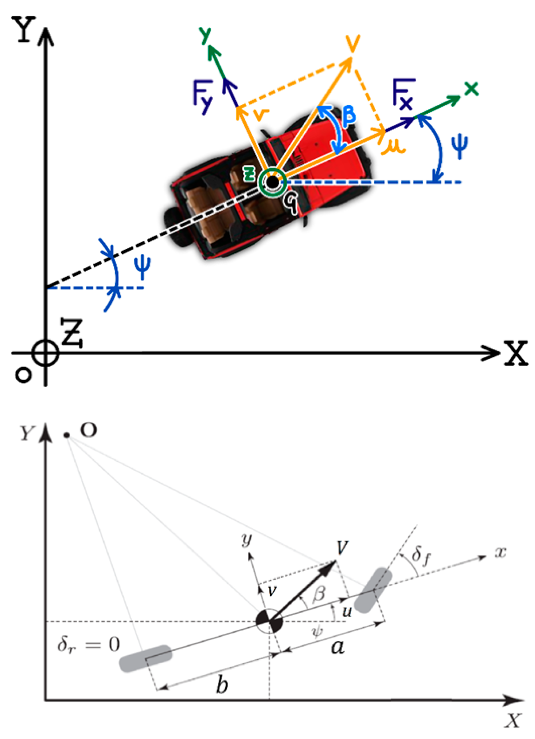
4.1. Lateral Dynamics Bicycle Model

The final section of this article is devoted to the study of the scaled numerical transfer functions. They can be obtained once the cornering stiffnesses measured at any asphalt temperature have been transposed to the reference one (25 °C). The computation of these corrected values is performed following the approach shown above. First, a simplified bicycle model [24] useful for comparing the analytical results coming from the transfer functions must be built. In such a model, both the front and the rear wheels are considered as if they were collapsed into a single entity. Operating in this way, it is possible to work with the “axle’s” properties and characteristics instead of those of the single wheels. A scheme of this configuration (where the most important angles to study the vehicle lateral dynamic behavior are indicated) is represented in the lower part of Figure 10.

a is the distance between the front axle and the vehicle center of gravity, b is the distance between the rear axle and the vehicle center of gravity, δ_f and δ_r are, respectively, the steering angle of the front and rear axle wheels (note: δ_f is equal to the steering wheel angle, δ_sw, divided by the steering ratio, str).

To develop this analysis, some assumptions about the open-loop model must be presented:

• The entire motion of the vehicle can be described along the XY plane.
• The vehicle is assumed to be rigid: the effects of the suspension system are neglected, and so roll and pitch motions are considered uncoupled from yaw motions.
• The contributions of aerodynamic forces are neglected. This can be done because the maximum speed reached by the vehicle during the maneuvers is always smaller than or equal to 120 km/h. Consequently, even if the aerodynamic force is proportional to the square of the velocity, the values that it assumes are small enough to be ignored without introducing large errors.
• The tire’s self-aligning stiffness—which is the influence of the related torque that is minor compared to the action of the other forces and moments involved—is neglected.

At this point, considering the upper scheme reported in Figure 10 and with reference to the (OXYZ) inertial frame, the equations of the motion of the vehicle are:

$$\{\begin{array}{c}m\ddot{X}=F_X\\ m\ddot{Y}=F_Y\\ J_z\ddot{\psi }=F_Z\end{array}$$

(17)

where $m$ is the vehicle mass and $J_z$ is its moment of inertia about the z-axis.

It is much more convenient to rewrite the equations of motion with reference to the local non-inertial frame (Gxyz) to better understand the dynamic behavior of the vehicle. In fact, by doing that:

• The generalized forces applied to the vehicle $\left(F_x,F_y, F_z, M_x, M_y, M_z\right)$ can be expressed quite simply;
• The trigonometric functions can be linearized because, except for the yaw angle, $\psi$, all the angles are assumed to be small.

Therefore, after some computation, Equation (18) becomes:

$$\{\begin{array}{c}m\left(\dot{u}-rv\right)=F_x\\ m\left(\dot{v}+ru\right)=F_y\\ J_z\dot{r}=M_z\end{array}$$

(18)

where $r$ is the yaw rate, which is the time derivative of the yaw angle, $\psi$.

Going on building the bicycle model it is possible, with some more calculations, to arrive to this formulation for $\dot{\beta }$ and $\dot{r}$:

$$\{\begin{array}{c}\dot{\beta }=\frac{-C_f-C_r}{mV}\beta +\frac{-a{C}_f+b{C}_r-mV}{m{V}^2}r+\frac{C_f}{mV}{\delta }_f\\ \dot{r}=\frac{-a{C}_f+b{C}_r}{J_z}\beta +\frac{-a^2{C}_f-b^2{C}_r}{J_{z}V}r+\frac{a{C}_f}{J_z}{\delta }_f\end{array}$$

(19)

Equation (19) can be easily rewritten in state space form. In fact, it is useful to be reminded that an LTI system like the one considered above can be defined through the following relations:

$$\begin{array}{c}\left\{\dot{z}\right\}=\left[A\right]\left\{z\right\}+\left[B\right]\left\{u\left(t\right)\right\}\\ \left\{y\right\}=\left[C\right]\left\{z\right\}+\left[D\right]\left\{u\left(t\right)\right\}\end{array}$$

(20)

where, in this case, being the state vector, $\left\{z\right\}$, equal to ${\left\{\begin{array}{cc}\beta & r\end{array}\right\}}^{\prime }$, the time derivative of the state vector, $\left\{\dot{z}\right\}$, equal to ${\left\{\begin{array}{cc}\dot{\beta }& \dot{r}\end{array}\right\}}^{\prime }$ and the input vector, $\left\{u\left(t\right)\right\}$, equal to $\left\{{\delta }_f\right\}$, the dynamic matrix, $\left[A\right]$, is equal to:

$$\left[A\right]=\left[\begin{array}{cc}\frac{-C_f-C_r}{mV}& \frac{-a{C}_f+b{C}_r-mV}{m{V}^2}\\ \frac{-a{C}_f+b{C}_r}{J_z}& \frac{-a^2{C}_f-b^2{C}_r}{J_{z}V}\end{array}\right]$$

(21)

the input gain matrix, $\left[B\right]$, is:

$$\left[B\right]=\left[\begin{array}{c}\frac{C_f}{mV}\\ \frac{a{C}_f}{J_z}\end{array}\right]$$

(22)

$\left[C\right]$ is defined as a 2 × 2 identity matrix while $\left[D\right]$ is a 2 × 1 all-zeros matrix. In order to compute the transfer functions describing the LTI system needed to develop the analysis in the frequency domain, $G_i$, it is necessary to introduce another important formula [36,37]:

$$G\left(s\right)=\left[C\right]{\left(s\left[I\right]-\left[A\right]\right)}^{-1}\left[B\right]+\left[D\right]$$

(23)

where $s$ is the Laplace variable ($=i\omega$, $\omega$ is the frequency) and $\left[I\right]$ is the identity matrix. By solving Equation (23), it is possible to obtain the expressions of $G_3$ and $G_2$:

$$G_3=\frac{\beta }{{\delta }_f}=\frac{\left(J_z{C}_{f}V\right)s+C_f{C}_{r}bl-m{C}_f{V}^{2}a}{\left(J_{z}m{V}^2\right)s^2+\left(mV\left(C_f{a}^2+C_r{b}^2\right)+J_{z}V\left(C_f+C_r\right)\right)s+C_f{C}_r{l}^2+m{V}^2\left(C_{r}b-C_{f}a\right)}$$

(24)

$$G_2=\frac{r}{{\delta }_f}=\frac{\left(m{C}_f{V}^{2}a\right)s+C_f{C}_{r}Vl}{\left(J_{z}m{V}^2\right)s^2+\left(mV\left(C_f{a}^2+C_r{b}^2\right)+J_{z}V\left(C_f+C_r\right)\right)s+C_f{C}_r{l}^2+m{V}^2\left(C_{r}b-C_{f}a\right)}$$

(25)

All the other required transfer functions related to lateral dynamics can be calculated as a combination of the fundamental ones, $G_3$ and $G_2$:

$$G_1=\frac{a_y}{{\delta }_f}=V\left(s{G}_3+G_2\right)$$

(26)

$$G_4=\frac{V·r}{a_y}=V\frac{G_2}{G_1}$$

(27)

$$G_5=\frac{{\alpha }_f}{{\delta }_f}=G_3+\frac{a}{V}{G}_2-1$$

(28)

$$G_6=\frac{{\alpha }_r}{{\delta }_f}=G_3-\frac{b}{V}{G}_2$$

(29)

4.2. Tire Relaxation Length

The tire relaxation length represents the reaction delay of the tire to the external input of a steering angle. Indeed, when a steering maneuver is operated, the fibers of the tires are stretched to generate the proper force; however, between the time instant at which the input (steering angle) is applied and the aimed force is generated, there exists a certain time delay. This interval is the one needed by the tire to deform and bring about the required force. This characteristic of the tire can be studied by applying the proper modifications to the vehicle lateral dynamics bicycle model described in the previous paragraph according to the following law:

$$\overline{{\alpha }_i}=\frac{1}{\overline{\sigma }s+1}{\alpha }_i$$

(30)

where ${\overline{\alpha }}_i$ is the true axle sideslip angle, $s$ is the Laplace variable ($=i\omega$) and $\overline{\sigma }$ is the averaged time constant, which is defined as the ratio between the relaxation length, $L_i$ (that is a parameter measured [m] during the experimental tests), and the forward vehicle velocity, $V$. Considering Equations (4) and (30) and taking into account the assumptions and steps made to build the model, the tire relaxation effect can be added by substituting $C_f$ and $C_r$ in Equations (24) and (25), respectively, with:

$$\overline{C_f}=\frac{1}{\overline{\sigma }s+1}{C}_f$$

(31)

$$\overline{C_r}=\frac{1}{\overline{\sigma }s+1}{C}_r$$

(32)

It is interesting to note that, with this formulation, the tire relaxation effect can be neglected again by simply making $L_i$ equal to zero.

4.3. Roll Motion Model

Assuming that the roll angle, $\varphi$, is small so that the trigonometric functions can be linearized, the general simplified expression that describes the vehicle roll motion on a level road is given below, in Equation (33):

$$\ddot{\varphi }=-\frac{K_{roll}}{J_x}\varphi -\frac{C_{roll}}{J_x}\dot{\varphi }+\frac{mh}{J_x}{a}_y$$

(33)

where $K_{roll}$ is the roll stiffness, $C_{roll}$ is the roll damping, $J_x$ is the vehicle moment of inertia about the x-axis and $h$ is the height of the roll center with respect to the ground. In this case, it is also possible to pass to the state space form of Equation (20). In fact, considering that $z_1$ is equal to $\varphi$, $z_2$ is equal to $\dot{\varphi }$ and $u\left(t\right)$ is equal to $a_y$, Equation (33) can be transformed into the following LTI system:

$$\{\begin{array}{c}{\dot{z}}_1=z_2\\ {\dot{z}}_2=-\frac{K_{roll}}{J_x}{z}_1-\frac{C_{roll}}{J_x}{z}_2+\frac{mh}{J_x}{a}_y\end{array}$$

(34)

Thus, being the state vector, $\left\{z\right\}$, equal to ${\left\{\begin{array}{cc}\varphi & \dot{\varphi }\end{array}\right\}}^{\prime }$, the time derivative of the state vector, $\left\{\dot{z}\right\}$, equal to ${\left\{\begin{array}{cc}\dot{\varphi }& \ddot{\varphi }\end{array}\right\}}^{\prime }$, and the input vector, $\left\{u\left(t\right)\right\}$, equal to $\left\{a_y\right\}$, the roll dynamic matrix, ${\left[A\right]}_{roll}$, is equal to:

$${\left[A\right]}_{roll}=\left[\begin{array}{cc}0& 1\\ -\frac{K_{roll}}{J_x}& -\frac{C_{roll}}{J_x}\end{array}\right]$$

(35)

the roll input gain matrix, ${\left[B\right]}_{roll}$, is:

$${\left[B\right]}_{roll}=\left[\begin{array}{c}0\\ \frac{mh}{J_x}\end{array}\right]$$

(36)

$C$_roll is defined as a 2 × 2 identity matrix while $D$_roll is a 2 × 1 zeros matrix. The procedure used to compute the two fundamental roll motion transfer functions, G7 (=ϕ/ay) and GVIII (=ϕ/ay=sG7) is exactly the same described previously for the lateral dynamics ones, G3 and G2. In this case, Equation (23) becomes:

$$G\left(s\right)={\left[C\right]}_{roll}{\left(s\left[I\right]-{\left[A\right]}_{roll}\right)}^{-1}{\left[B\right]}_{roll}+{\left[D\right]}_{roll}$$

(37)

The roll motion transfer functions that will be studied in the following paragraphs are:

$$G_7=\frac{\varphi }{a_y}=\frac{mh}{J_x{s}^2+C_{roll}s+K_{roll}}$$

(38)

$$G_8=\frac{\varphi }{{\delta }_f}=G_7·G_1$$

(39)

$$G_9=\frac{\dot{\varphi }}{{\delta }_f}=s{G}_7·G_1$$

(40)

4.4. Computation of the Updated Numerical Transfer Functions

The last step consists in computing the updated numerical transfer function values. The procedure adopted is a company-consolidated standard and is quite complex. Concerning the lateral dynamics curves, the starting point is the calculation of an analytical delta which can be obtained at every frequency level, as follows:

$${\Delta }_i=analytical scaled tf-analytical original tf$$

(41)

Each ${\Delta }_i$ is a vector of complex numbers that must be converted from the Gain-Phase format to the Real-Imaginary Part format. After that, the deltas can be applied directly to the original numerical transfer functions, which are computed by multiplying the corresponding cross-spectra and auto-spectra (as usual, this information is contained in the experimental test output file). This situation is represented by Equations (42)–(46):

$$G_1^{\prime }=\frac{a_y}{{\delta }_{sw}}=\left(cross-sprectrum\left(\frac{a_y}{{\delta }_{sw}}\right)/auto-spectum\left({\delta }_{sw}\right)\right)+{\Delta }_1$$

(42)

$$G_2^{\prime }=\frac{r}{{\delta }_{sw}}=\left(cross-sprectrum\left(\frac{r}{{\delta }_{sw}}\right)/auto-spectum\left({\delta }_{sw}\right)\right)+{\Delta }_2$$

(43)

$$G_3^{\prime }=\frac{\beta }{{\delta }_{sw}}=\left(cross-sprectrum\left(\frac{\beta }{{\delta }_{sw}}\right)/auto-spectum\left({\delta }_{sw}\right)\right)+{\Delta }_3$$

(44)

$$G_5^{\prime }=\frac{{\alpha }_f}{{\delta }_{sw}}=\left(cross-sprectrum\left(\frac{{\alpha }_f}{{\delta }_{sw}}\right)/auto-spectum\left({\delta }_{sw}\right)\right)+{\Delta }_4$$

(45)

$$G_6^{\prime }=\frac{{\alpha }_r}{{\delta }_{sw}}=\left(cross-sprectrum\left(\frac{{\alpha }_r}{{\delta }_{sw}}\right)/auto-spectum\left({\delta }_{sw}\right)\right)+{\Delta }_5$$

(46)

Then, the resulting complex numbers can be brought back to the Gain-Phase format, and the remaining lateral dynamics transfer function, $G_4^{\prime }$, can be obtained as a combination of $G_2^{\prime }$ and $G_1^{\prime }$:

$$G_4^{\prime }=\frac{V·r}{a_y}: \{\begin{array}{c}gain\left(G_4^{\prime }\right)=V·\frac{gain\left(G_2^{\prime }\right)}{gain\left(G_1^{\prime }\right)}\\ phase\left(G_4^{\prime }\right)=phase\left(G_2^{\prime }\right)-phase\left(G_1^{\prime }\right)\end{array}$$

(47)

This conversion and re-conversion operation can seem trivial, but it has been proved to lead to more robust results. Instead, for the three curves representing the roll motion, all the operations are done directly in the Gain-Phase format as follows:

$$G_7^{\prime }=\frac{\varphi }{a_y}: no changes wrt the original numerical values$$

(48)

$$G_8^{\prime }=\frac{\varphi }{{\delta }_{sw}}: \{\begin{array}{c}gain\left(G_8^{\prime }\right)=gain\left(G_7^{\prime }\right)·gain\left(G_1^{\prime }\right)\\ phase\left(G_8^{\prime }\right)=phase\left(G_7^{\prime }\right)+phase\left(G_1^{\prime }\right)\end{array}$$

(49)

$$G_9^{\prime }=\frac{\dot{\varphi }}{{\delta }_{sw}}: \{\begin{array}{c}gain\left(G_9^{\prime }\right)=gain\left(G_8^{\prime }\right)·\left(2\pi s\right) \\ phase\left(G_9^{\prime }\right)=phase\left(G_8^{\prime }\right)+90° \end{array}$$

(50)

Basically, the first transfer function is left unchanged, the second one is computed as a combination of $G_7^{\prime }$ and $G_1^{\prime }$ while the third one is obtained deriving $G_8^{\prime }$ in the frequency domain. Finally, a new set of curves related to the steering wheel torque, $C_{sw}$, can be introduced. Moreover, these transfer functions are defined from the beginning in the Gain-Phase format with the following expressions:

$$G_{11}^{\prime }=\frac{a_y}{C_{sw}}: no changes wrt the original numerical values$$

(51)

$$G_{10}^{\prime }=\frac{{\delta }_{sw}}{C_{sw}}: \{\begin{array}{c}gain\left(G_{10}^{\prime }\right)=\frac{gain\left(G_{11}^{\prime }\right)}{gain\left(G_1^{\prime }\right)}\\ phase\left(G_{10}^{\prime }\right)=phase\left(G_{11}^{\prime }\right)-phase\left(G_1^{\prime }\right)\end{array}$$

(52)

$$G_{12}^{\prime }=\frac{r}{C_{sw}}: \{\begin{array}{c}gain\left(G_{12}^{\prime }\right)=gain\left(G_{10}^{\prime }\right)·gain\left(G_2^{\prime }\right)\\ phase\left(G_{12}^{\prime }\right)=phase\left(G_{10}^{\prime }\right)+phase\left(G_2^{\prime }\right)\end{array}$$

(53)

Again, while the first transfer function is not modified, the second and third ones are computed as a combination of $G_{11}^{\prime }$–$G_1^{\prime }$ and $G_{10}^{\prime }$–$G_2^{\prime }$, respectively.

4.5. Analysis of the Scaled Numerical Results

In conclusion, having seen the methodology to scale the numerical transfer functions, some results can be presented. The details about the case and the curves considered in Figure 11 and Figure 12 are summarized in

Table 2. Numerical transfer functions rescaling; details of the curves considered.

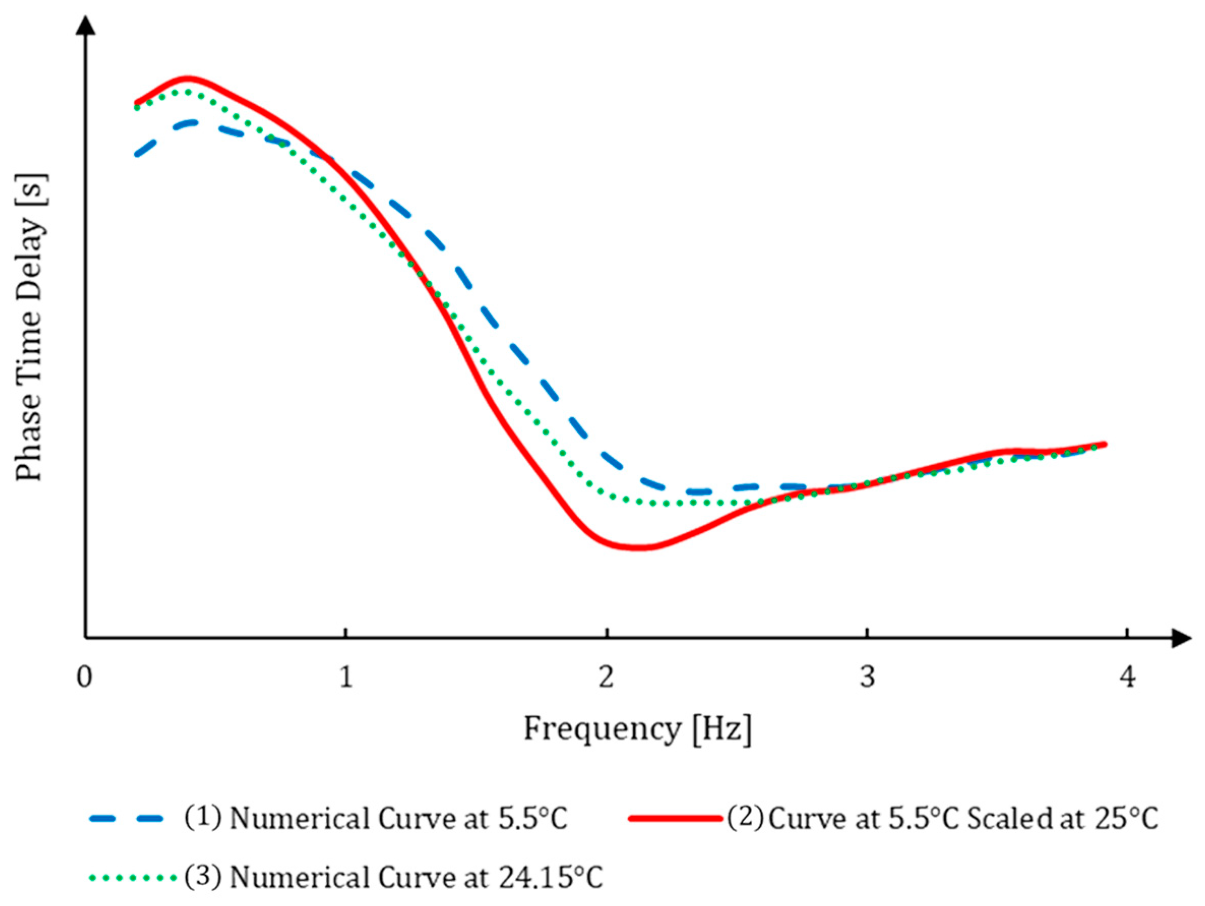
${\mathit{G}}_{\mathbf{2}}^{\mathbf{\prime }}$ (Figure 11)
Curve ID	Vehicle	Temperature	Maneuver	Cornering Stiffnesses
#1—Blue	B-Segment Hybrid Subcompact Crossover SUV	5.5 °C	Frequency Sweep, 0.5 g $a_y$	Measured
#2—Red	B-Segment Hybrid Subcompact Crossover SUV	25 °C	Frequency Sweep, 0.5 g $a_y$	Computed
#3—Green	B-Segment Hybrid Subcompact Crossover SUV	24.15 °C	Frequency Sweep, 0.5 g $a_y$	Measured
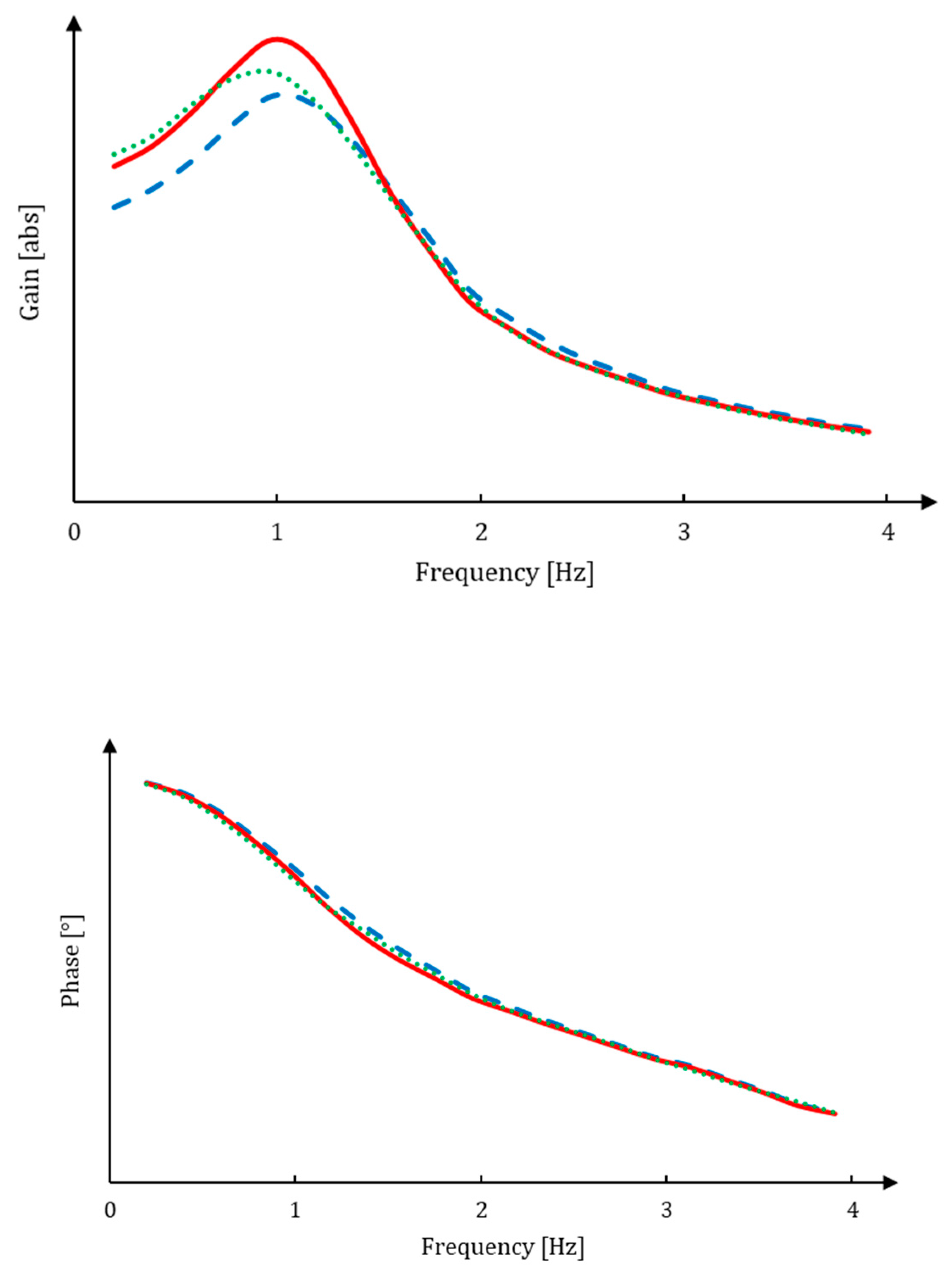
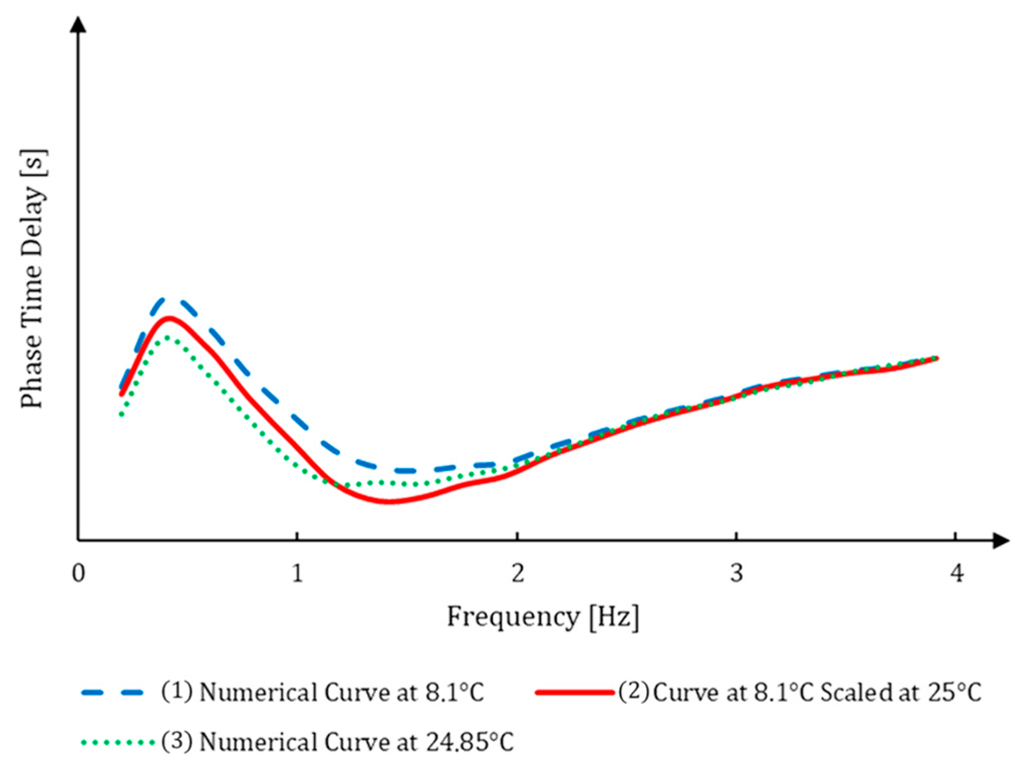
${\mathit{G}}_{\mathbf{3}}^{\mathbf{\prime }}$ (Figure 12)
Curve ID	Vehicle	Temperature	Maneuver	Cornering Stiffnesses
#1—Blue	B-Segment Subcompact Crossover SUV	8.1 °C	Frequency Sweep, 0.5 g $a_y$	Measured
#2—Red	B-Segment Subcompact Crossover SUV	25 °C	Frequency Sweep, 0.5 g $a_y$	Computed
#3—Green	B-Segment Subcompact Crossover SUV	24.85 °C	Frequency Sweep, 0.5 g $a_y$	Measured

.

Curve #2 is obtained by applying the cornering stiffness correction in temperature to the measured values of curve #1 and then employing the abovementioned bicycle model. Curve #3 is used to verify the accuracy of the re-scalation. Obviously, the closer the red and green curves, the better the results will be. The input data necessary to run the overall MatLab script can be found in the output file generated after an experimental test is executed. In particular, in both these cases the reference maneuver used to select all the values of the variables is that of curve #1 in Table 2.

The graphs in Figure 11 and Figure 12 show, respectively, a comparison of the yaw rate and the steering wheel angle numerical transfer function ($G_2^{\prime }$), and a comparison of the sideslip angle and the steering wheel angle numerical transfer function ($G_3^{\prime }$) for two different vehicles that were tested in a frequency range up to 4 Hz.

The gain, phase and phase time delay have been plotted. As can be seen, the results are good at every frequency level, even if the peak value for the gain of the corrected curves at 25 °C is overestimated for both the transfer functions considered here. Indeed, this tendency has been spotted in the majority of the cases studied. In

Table 3. Numerical transfer functions, gain and phase time delay at fixed frequencies.

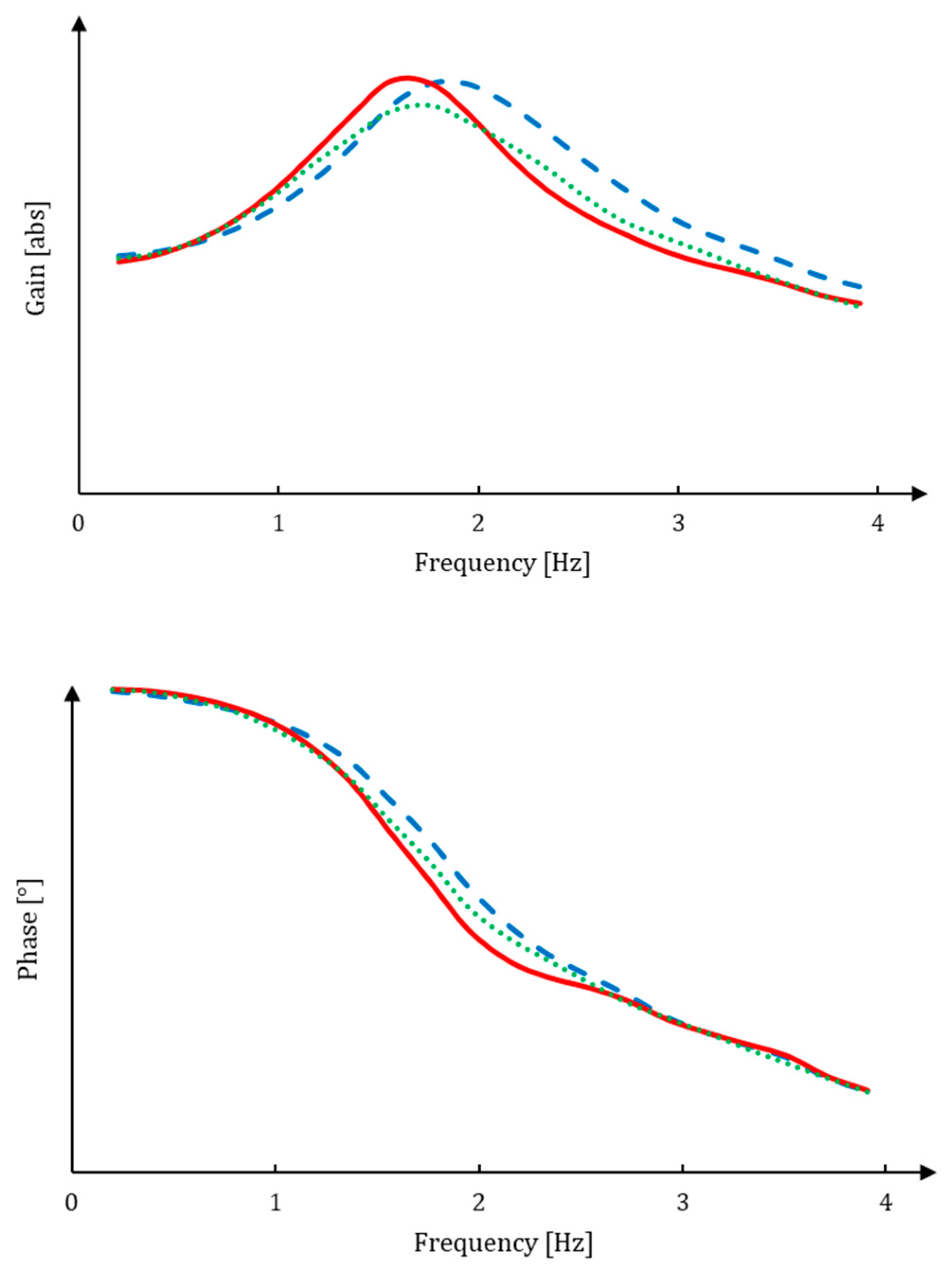
B-Segment Hybrid Subcompact Crossover SUV, Frequency Sweep, 0.5 g ${\mathit{a}}_{\mathit{y}}$, ${\mathit{G}}_{\mathbf{3}}^{\mathbf{\prime }}$ (=$\mathit{\beta }\mathbf{/}{\mathit{\delta }}_{\mathit{s}\mathit{w}}$)
Component	Frequency	Value Measured at 5.5 °C	Value Computed at 25 °C	Value Measured at 24.15 °C
Gain	≈ 0 Hz	0.021 [-]	0.027 [-]	0.025 [-]
Phase Delay		−0.144 [s]	−0.153 [s]	−0.184 [s]
Gain	0.5 Hz	0.022 [-]	0.028 [-]	0.026 [-]
Phase Delay		−0.113 [s]	−0.130 [s]	−0.140 [s]
Gain	1 Hz	0.025 [-]	0.032 [-]	0.029 [-]
Phase Delay		−0.137 [s]	−0.156 [s]	−0.164 [s]
B-Segment Subcompact Crossover SUV, Frequency Sweep, 0.5 g ${\mathit{a}}_{\mathit{y}}$, ${\mathit{G}}_{\mathbf{2}}^{\mathbf{\prime }}$ (=$\mathit{r}\mathbf{/}{\mathit{\delta }}_{\mathit{s}\mathit{w}}$)
Component	Frequency	Value Measured at 5.5 °C	Value Computed at 25 °C	Value Measured at 24.15 °C
Gain	1 Hz	0.391 [-]	0.412 [-]	0.400 [-]
Phase Delay		−0.064 [s]	−0.072 [s]	−0.082 [s]
Gain	1.5 Hz	0.385 [-]	0.363 [-]	0.363 [-]
Phase Delay		−0.113 [s]	−0.122 [s]	−0.116 [s]
Gain	2 Hz	0.307 [-]	0.284 [-]	0.290 [-]
Phase Delay		−0.116 [s]	−0.119 [s]	−0.118 [s]

, there are some additional examples, at different frequency levels, for the same two vehicles of the previous comparisons. The correct estimation of the numerical transfer functions values at 25 °C when the frequency is low and fixed is the most important task that the tool must accomplish. In doing that, it behaves very well and provides satisfactory results.

5. Conclusions

Looking at the graphs reported in Figure 11 and Figure 12 and the data in Table 3 and considering the rest of the analysis that was carried out, it is possible to conclude that the numerical scaled curve values approximate in a useful way those of the original curve close to 25 °C. This is true of all the transfer functions and the different cases studied, particularly at low frequencies (<2 Hz). It is useful to underline again that these results were achieved with a tool that requires only one experimental measurement to perform a temperature correction. A little bit of accuracy has been lost, but it is a matter of compromise: the tool is quite simple, robust and efficient. These are competing needs, and an excellent equilibrium point between all of them has been found.

There are three points that could be really interesting to face in order to further develop this project: First, it would be useful to extend the analysis to other vehicle categories, like commercial vehicles or sportscars, and check the validity of the tool. In fact, this entire study was built around similar passenger cars that mount tires with analogue compound characteristics and geometrical dimensions. In particular, most of them are compact SUVs. The second point is that it would be useful to conduct a deep study of the behavior of different tires, such as winter tires, low rolling resistance tires, etc. Last, it could be interesting to conduct an analysis to understand what happens with maneuvers executed approaching limit conditions, i.e., when the lateral acceleration is close to limit value.

References

- Wang, S.; Al Atat, H.; Ghaffari, M.; Lee, J.; Xi, L.-F. Prognostics of automotive sensors: Tools and case study. Failure Prevention for System Availability. In Proceedings of the 62nd Meeting of the Society for Machinery Failure Prevention Technology, Virginia Beach, VA, USA, 6–8 April 2008. [Google Scholar]
- Armstrong, K.; Das, S.; Cresko, J. The energy footprint of automotive electronic sensors. Sustain. Mater. Technol. 2020, 25, e00195. [Google Scholar] [CrossRef]
- De Novellis, L.; Sorniotti, A.; Gruber, P.; Shead, L.; Ivanov, V.; Hoepping, K. Torque Vectoring for Electric Vehicles with Individually Controlled Motors: State-of-the-Art and Future Developments. World Electr. Veh. J. 2012, 5, 617–628. [Google Scholar] [CrossRef] [Green Version]
- Manca, R.; Castellanos Molina, L.M.i.; Hegde, S.; Tonoli, A.; Amati, N.; Pazienza, L. Optimal Torque-Vectoring Control Strategy for Energy Efficiency and Vehicle Dynamic Improvement of Battery Electric Vehicles with Multiple Motors; SAE Technical Paper 2023-01-0563. In Proceedings of the WCX SAE World Congress Experience, Detroit, MI, USA, 18–20 April 2023. [Google Scholar] [CrossRef]
- Ferraris, A.; De Cupis, D.; de Carvalho Pinheiro, H.; Messana, A.; Sisca, L.; Airale, A.G.; Carello, M. Integrated Design and Control of Active Aerodynamic Features for High Performance Electric Vehicles; SAE Technical Paper 2020-36-0079. In Proceedings of the 2020 SAE Brasil Congress & Exhibition, Sao Paulo, Brazil, 1 December 2021. [Google Scholar] [CrossRef]
- de Carvalho Pinheiro, H.; Punta, E.; Carello, M.; Ferraris, A.; Airale, A.G. Torque Vectoring in Hybrid Vehicles with In-Wheel Electric Motors: Comparing SMC and PID control. In Proceedings of the 2021 IEEE International Conference on Environment and Electrical Engineering and 2021 IEEE Industrial and Commercial Power Systems Europe (EEEIC/I&CPS Europe), Bari, Italy, 7–10 September 2021; pp. 1–6. [Google Scholar] [CrossRef]
- Carello, M.; Ferraris, A.; Carvalho Pinheiro H de Cruz Stanke, D.; Gabiati, G.; Camuffo, I.; Grillo, M. Human-Driving Highway Overtake and Its Perceived Comfort: Correlational Study Using Data Fusion; SAE Technical Paper 2020-01-1036. In Proceedings of the WCX SAE World Congress Experience, Detroit, MI, USA, 21–23 April 2020. [Google Scholar] [CrossRef]
- Dingyi, Y.; Haiyan, W.; Kaiming, Y. State-of-the-art and trends of autonomous driving technology. In Proceedings of the 2018 IEEE International Symposium on Innovation and Entrepreneurship (TEMS-ISIE), Beijing, China, 30 March–1 April 2018; pp. 1–8. [Google Scholar] [CrossRef]
- Tramacere, E.; Luciani, S.; Feraco, S.; Bonfitto, A.; Amati, N. Processor-in-the-Loop Architecture Design and Experimental Validation for an Autonomous Racing Vehicle. Appl. Sci. 2021, 11, 7225. [Google Scholar] [CrossRef]
- Yunzheng, Z.; Shaofei, Q.; Huang, A.C.; Jianhong, X. Smart Vehicle Control Unit—An integrated BMS and VCU System. IFAC-Pap. 2018, 51, 676–679. [Google Scholar] [CrossRef]
- de Carvalho Pinheiro, H.; Carello, M. Design and validation of a high-level controller for automotive active systems. SAE Int. J. Veh. Dyn. Stab. NVH 2022, 7, 83–98. [Google Scholar] [CrossRef]
- Dugoff, H.; Fancher, P.S.; Segel, L. An Analysis of Tire Traction Properties and Their Influence on Vehicle Dynamic Performance. SAE Trans. 1970, 79, 1219–1243. [Google Scholar]
- Pacejka, H.B. Analysis of Tire Properties. In Mechanics of Pneumatic Tires; Clark, S.K., Ed.; National Highway Traffic Safety Administration: Washington, DC, USA, 1981; pp. 721–870. [Google Scholar]
- Farroni, F.; Russo, M.; Russo, R.; Terzo, M.; Timpone, F. A combined use of phase plane and handling diagram method to study the influence of tyre and vehicle characteristics on stability. Veh. Syst. Dyn. 2013, 51, 1265–1285. [Google Scholar] [CrossRef]
- Farroni, F. TRICK-Tire/Road Interaction Characterization & Knowledge—A tool for the evaluation of tire and vehicle performances in outdoor test sessions. Mech. Syst. Signal Process. 2016, 72–73, 808–831. [Google Scholar] [CrossRef]
- Farroni, F.; Sakhnevych, A.; Timpone, F. Physical modelling of tire wear for the analysis of the influence of thermal and frictional effects on vehicle performance. Proceedings of the Institution of Mechanical Engineers, Part L. J. Mater. Des. Appl. 2017, 231, 151–161. [Google Scholar] [CrossRef]
- Stellantis Media Official Website. Available online: https://www.media.stellantis.com/em-en/fca-archive/press/fca-what-s-behind-episode-3-balocco-proving-ground (accessed on 1 January 2022).
- Michelin Website. Available online: https://www.michelinman.com/auto/tips-and-advice/advice-auto/tires-101/how-are-tires-made (accessed on 1 January 2022).
- U.S. Tire Manufacturers Association Website. Available online: https://www.ustires.org/whats-tire-0 (accessed on 1 June 2023).
- European Tyre & Rubber Manufacturer’s Association. The ETRMA Statistics Report Edition 2015. Available online: https://www.etrma.org/wp-content/uploads/2019/09/20151214-statistics-booklet-2015-final2.pdf (accessed on 1 June 2023).
- Angrick, C.; van Putten, S.; Prokop, G. Influence of Tire Core and Surface Temperature on Lateral Tire Characteristics. SAE Int. J. Passeng. Cars-Mech. Syst. 2014, 7, 468–481. [Google Scholar] [CrossRef]
- Lugaro, C.; Alirezaei, M.; Konstantinou, I.; Behera, A. A Study on the Effect of Tire Temperature and Rolling Speed on the Vehicle Handling Response. SAE Technical Paper 2020-01-1235. In Proceedings of the WCX SAE World Congress Experience, Detroit, MI, USA, 21–23 April 2020. [Google Scholar]
- Genta, G.; Morello, L. The Automotive Chassis; Springer: Berlin/Heidelberg, Germany, 2009; Volume 1. [Google Scholar]
- Milliken, W.F. Race Car Vehicle Dynamics. In Society of Automotive Engineers; SAE International: Warrendale, PA, USA, 1995; ISBN 978-0-7680-0103-7. [Google Scholar]
- Ejsmont, J.; Taryma, S.; Ronowski, G. Swieczko-Zurek Mechanical Faculty. Influence of Temperature on the Tire Rolling Resistance. SAE Int. J. Automot. Technol. 2018, 19, 45–54. [Google Scholar] [CrossRef]
- Lu, D.; Lu, L.; Wu, H.; Li, L.; Wang, W.; Lv, M. Study on the Influence of Temperature on Tire Cornering Stiffness and Aligning Stiffness; Preprint (Version 1); Research Square: Durham, UK, 26 June 2020. [Google Scholar] [CrossRef]
- Okubo, R.; Oyama, K. Effects of Tire Thermal Characteristics on Vehicle Performance. In Proceedings of the FISITA 2014 World Automotive Congress, Maastricht, The Netherlands, 2–6 June 2014. [Google Scholar]
- Behera, A. The Influence of Tire Temperature and Velocity on Vehicle Dynamics. Master’s Thesis, Eindhoven University of Technology, Eindhoven, The Netherlands, 2019. [Google Scholar]
- Pacejka, H.B. Tire and Vehicle Dynamics, 3rd ed.; Butterworth-Heinemann: Oxford, UK, 2012. [Google Scholar]
- ISO 7401:2011; Road Vehicles—Lateral Transient Response Test Methods—Open-Loop Test Methods. International Organization for Standardization: Geneva, Switzerland, 2011.
- ISO/TR 8725:1988; Road Vehicles—Transient Open-Loop Response Test Method with One Period of Sinusoidal Input. Available online: https://www.iso.org/standard/16128.html (accessed on 1 June 2023).
- Dörrie, H.; Schröder, C.; Wies, B. Winter Tires: Operating Conditions, Tire Characteristics and Vehicle Driving Behavior. Tire Sci. Technol. 2010, 38, 119–136. [Google Scholar] [CrossRef]
- Farroni, F. Tire/Road Interaction Models. In Analysis of the Results Provided by a Grip and Thermodynamic-Sensitive Tire/Road Interaction Force Characterization Procedure; Tire Technology International: Surrey, UK, 2014. [Google Scholar]
- Warasitthinon, N.; Robertson, C.G. Interpretation of the tanδ Peak Height for Particle-Filled Rubber and Polymer Nanocomposites with Relevance to Tire Tread Performance Balance. Rubber Chem. Technol. 2018, 91, 577–594. [Google Scholar] [CrossRef]
- Rodríguez-Guadarrama, L.; Kounavis, J.; Maldonado, J. Functionalization: A Key Differential Factor in the Design of SSBRs for High Performance Tires; 194th Technical Meeting; Rubber World: Akron, OH, USA, 2018. [Google Scholar]
- Kalman, R. On the general theory of control systems. IRE Trans. Autom. Control 1959, 4, 110. [Google Scholar] [CrossRef]
- Canuto, E.; Novara, C.; Colangelo, L. Embedded model control: Reconciling modern control theory and error-based control design. Control Theory Technol. 2018, 16, 261–283. [Google Scholar] [CrossRef]