Inverse Kinematics of Robot Manipulator Based on BODE-CS Algorithm

Abstract

Differential evolution is a popular algorithm for solving global optimization problems. When tested, it has reportedly outperformed both robotic problems and benchmarks. However, it may have issues with local optima or premature convergence. In this paper, we present a novel BODE-CS (Bidirectional Opposite Differential Evolution–Cuckoo Search) algorithm to solve the inverse kinematics problem of a six-DOF EOD (Explosive Ordnance Disposal) robot manipulator. The hybrid algorithm was based on the differential evolution algorithm and Cuckoo Search algorithm. To avoid any local optimum and accelerate the convergence of the swarm, various strategies were introduced. Firstly, a forward-kinematics model was established, and the objective function was formulated according to the structural characteristics of the robot manipulator. Secondly, a Halton sequence and an opposite search strategy were used to initialize the individuals in the swarm. Thirdly, the optimization algorithms applied to the swarm were dynamically allocated to the Differential Evolution algorithm or the Cuckoo algorithm. Fourthly, a composite differential algorithm, which consisted of a dynamically opposite differential strategy, a bidirectional search strategy, and two other typically used differential strategies were introduced to maintain the diversity of the swarm. Finally, two adaptive parameters were introduced to optimize the amplification factor F and cross-over probability C_r. To verify the performance of the BODE-CS algorithm, two different tasks were tested. The experimental results of the simulation showed that the BODE-CS algorithm had high accuracy and a fast convergence rate, which met the requirements of an inverse solution for the manipulator.

1. Introduction

Robotics have integrated many achievements in theoretical knowledge and technology, including controls [1], artificial intelligence [2], and complex mechanisms [3], etc. To solve the problem of path planning, motion control, and trajectory tracking, among others, a kinematic analysis is necessary. It includes forward and inverse kinematics, where forward kinematics [4] describe the process of obtaining the end-effector’s position and orientation by using the relative configurations of each pair of adjacent links, and inverse kinematics describe the process of obtaining a set of joint variables based on the desired position and orientation. The inverse kinematics of the manipulator play an important role in robotic research.The desired trajectory can be transformed via inverse kinematics into the corresponding joint trajectories [5]. It is also the fundamental technology for solving many problems, such as trajectory tracking [6], object grasping [7], and dynamic analysis [8]. It allows for the joint variables associated with the required task to be determined. The IK (inverse kinematics) problem is a complex coupling problem. Many methods have been proposed that can be divided into three categories: analytical solutions (closed-form solutions) [9], numerical solutions [10], and intelligent algorithms [11]. Regarding the analytical solutions, they consist of algebraic and geometric aspects [12]. For example, Gan et al. [13] proposed a complete analytical solution for the inverse kinematics of a P2Arm robotic arm. The method provided the robot arm access to any position in an undefined environment. However, traditional closed-form methods are difficult to implement in robots with particular geometric features. The joint variables of numerical solutions are obtained for iterative computational procedures. This has been the main approach for resolving the IK problem of complex articulated manipulators. Unfortunately, traditional numerical methods, such as pseudo-inverse methods [14], the Newton method [15], and so forth, are time-consuming [16]. The Jacobian IK method, with its complex matrix calculations and singularity issues, has made the problem difficult to solve. Similar to the Jacobian IK method, the iteration of the Newton method is complex and difficult to implement. Due to the problems with the Jacobian and Newton methods, various intelligent algorithms have been proposed, such as the GA (Genetic Algorithm) [17,18], PSO (Particle Swarm Optimization) [19], DE (Differential Evolution) [20], NN (Neural Networks) [21], ABC (Artificial Bee Colony) [22], and ACS (Ant Colony System) [23]. The main idea involved in using intelligent algorithms for solving inverse kinematics is to transform the problem into minimizing or maximizing a fitness function with an iterative strategy. The comparison of the algorithms is shown as

Table 1. A comparison of different algorithms in terms of their advantages, disadvantages, and limitations.

	Advantages	Disadvantages	Limitation
DE [24]	fast convergence, strong robustness, and easy to hybridize with other algorithms	easily influenced by local optima, premature convergence, and even search stagnation	lack of theoretical analysis of convergence
PSO [25]	fast convergence, few control parameters, strong robustness	easily influenced by local optima, premature convergence	poor discrete optimization results
CS [26]	few control parameters, convergence, hard to fall into the local optimal, easy to hybridize with other algorithms, strong global search ability.	slow convergence rate and lack of vitality	difficult to set the search step-size; better individuals may be discarded in the search process; poor local search ability
ACS [27]	strong robustness; easy to hybridize with other algorithms	time intensive, slow convergence rate, and easily influenced by local optimum	weak ability to balance the population diversity and convergence rate
ABC [28]	high global search ability, simple parameter setting, and wide range of application	slow convergence low precision	sensitive to parameter setting
NN [29]	highly parallelized, robust, and fault tolerant	sensitive to data quality and noise; requires a lot of data and computing resources	the learning process cannot be explained, and the computing rate of neural network is slow
GA [30]	strong explore ability, suitable for nonlinear problems, hard to fall into local optimum	the programming is complicated to implement, and easy to fall into local optimal solutions	the results is very dependent on the encoding scheme; the convergence speed is slow; and the parameter adjustment is difficult

.

The Differential Evolution (DE) algorithm is an intelligent optimization algorithm, which was proposed by Price and Storn [31]. It has many appealing characteristics, such as fast convergence, few control parameters, and excellent robustness. It has commonly been used to optimize engineering problems, such as signal processing [32], satellite image enhancement [33], and numerical optimization [34]. In the robotic area, DE algorithms and their variants have been widely used in motion planning [35], path trajectory [36], visual control [37], and so on. A novel DE algorithm was proposed by Ren et al. [38] to plan a minimum-acceleration trajectory for a humanoid robot. The results indicated that the improved DE algorithm was effective in generating the minimum-acceleration trajectory for the humanoid robot with a seven-DOF manipulator. Zhang et al. [39] proposed a multi-objective algorithm that hybridized the DE algorithm with a PSO. The path length, the degree of safety, and the degree of smoothness were taken as the objectives to optimize. The experiment results revealed that the hybrid algorithm outperformed other algorithms on the path length, the degree of safety, and the degree of smoothness. Cuckoo Search (CS) is a novel search algorithm proposed by Yang and Deb. It is a widely used algorithm that has less computational demand, and it can be easily merged into other algorithms. Due to its simplistic mathematical process, it has been used in multi-objective optimization [40], neural networks [41], facial recognition [42], and so on. Similar to the DE algorithm, the CS has also been widely used in robotics for such applications as trajectory tracking [43], path planning [44], and so forth. Sharm et al. [45] used a tournament selection function, which considered both path time and length, to optimize the CS algorithm for robot path planning. Compared to the PSO and the traditional CS, the performance of Sharm’s improved CS algorithm was better in terms of path length and time optimization. To obtain a higher efficiency and an automated trajectory, the Adaptive Cuckoo Search (ACS) was proposed by Zhang et al. [46] In the algorithm, the path time was minimized under strict dynamic constraints. Compared to other algorithms, the ACS algorithm had better performance, with a better convergence speed and greater efficiency. Karahan et al. [47] presented a novel trajectory generation method that considered time optimization, jerk optimization, and time–jerk optimization. The improved CS was proposed and compared to earlier studies, and the results showed that the improved CS was more effective than other algorithms. Despite the significant advantages of the DE and CS algorithms, they are easily influenced by local optima with low convergence accuracy. Although many variants of the DE algorithm have been proposed, a single-mutation strategy has often been unable to solve complex optimization problems; it is also difficult for the basic DE algorithm to balance the global exploration ability and local development ability. Meanwhile, they usually focused on optimizing the cross-over probabilities and mutation factors. The quality of the initial swarm and the weight coefficient in the fitness function has a significant influence on the results, which is typically ignored. Additionally, if the swarm size is small, the risk of premature convergence with a DE algorithm increases. To solve the problems and improve the accuracy and performance of DE algorithms, we proposed a novel hybrid algorithm: the Bidirectional Opposite Differential Evolution–Cuckoo Search (BODE-CS) algorithm. The contributions of this study are summarized in the following:

(1)

A novel objective function was formulated according to the structural characteristics of the robot manipulator. By using the D–H (Denavit–Hartenberg) method, the pose matrix of the robot end effector was analyzed. Then, a novel objective function was proposed to accelerate the algorithm’s convergence rate. The objective function considered both the position error and orientation error. The coefficient of the orientation error was associated with link length, link twist angle, link offset, and joint angle, etc.

(2)

A Halton sequence and the opposite strategy were used to initialize the swarm. A Halton sequence with a low difference was proposed to initialize the swarm instead of the random initialization method. The Halton sequence could improve the diversity of the swarm and enable the individuals to be more evenly distributed. Meanwhile, the opposite strategy was also applied to optimize the swarm quality.

(3)

A multi-strategy composite DE algorithm with improved factors was formulated. To avoid the local optimum, firstly, a dynamical opposite differential evolution algorithm and bidirectional search strategies were introduced. Since the maximum and minimum values of each dimension were dynamically changed during the iterative process, a smaller search range was more conducive to algorithm convergence. Therefore, the maximum and minimum values of each dimension were selected as new boundaries for generating new individuals. Then, by adjusting the differential evolution formula symbols, new bidirectional individuals could be generated. Based on the proposed two strategies, two typical DE mutation strategies were also introduced to form and enhance a new multi-strategy composite DE algorithm. Finally, the amplification factor (F) in mutation and the cross-over probability factor ($C_r$) were both improved.

(4)

A multi-strategy CS algorithm was constructed. During the CS algorithm’s operation, the dynamically opposite strategy, linear global best strategy, improved step strategy, and linear decreasing abandonment strategy were applied. The linear global best strategy considered both the current individual and the global best individual. A weighted method was used to combine them in order to accelerate the swarm convergence. An improved step strategy was used to increase the diversity of the swarm, and the linear decreasing abandonment strategy could improve the diversity at the beginning of searching, as well as increased probability to retain the best individual at the end of searching.

(5)

The mechanism for selecting the best algorithm and strategy was established for the BODE-CS algorithm. First, the BODE algorithm and improved CS algorithm were dynamically selected by an algorithm selection function. Then, a piece-wise function was formulated to choose one strategy for the BODE algorithm and optimize the swarm. Meanwhile, the dynamically opposite strategy and the best linear global strategy were also applied to improve the CS algorithm.

The remainder of this paper is organized as follows: In Section 2, the kinematic model of our robot’s end effector is established, and a novel objective function is formulated. Then, in Section 3, the procedures of the traditional DE algorithm and CS algorithm are introduced. Additionally, the improved strategies for DE and CS are also introduced to accelerate convergence and mitigate the influence of the local optima. In Section 4, the simulations are described, and the comparative results of the BODE-CS algorithm are presented. Finally, the conclusion and perspectives are provided in Section 5.

2. Kinematic Analysis for the Robot Manipulator

2.1. Mathematical Model of the Manipulator

Each joint is associated with a joint variable q. The expression of variable q is as follows:

$$q={[q_1{q}_2\dots q_n]}^T,$$

(1)

where ${\mathit{q}}_i$ represents the $i_{th}$ joint variable; in the case of a revolute joint, the variable $q_i$ is the angle ofrotation, and, in the case of a prismatic joint, it is the joint displacement [48]. n represents the number of DOFs.

The homogeneous transformation matrix is used to describe the position and orientation of one coordinate system in another coordinate system. It is used to change the reference frame in which a vector or frame is represented [49]. The superscript of the matrix indicates the reference coordinate system; the subscript right corner of the matrix identifies the target coordinate system. It includes a translation matrix ${\mathbf{P}}_{3\times 1}$, a rotation matrix ${\mathbf{R}}_{3\times 3}$, and a $1\times 4$ matrix (0, 0, 0, 1). According to the D–H method, the homogeneous transformation matrix ${\mathbf{A}}_i^{i-1}$ could be obtained through the following:

$$\begin{array}{c}\hfill \begin{array}{cccc}\hfill {\mathbf{A}}_i^{i-1}& =\hfill & \hfill & Ro{t}_{z,{\theta }_i}Tran{s}_{z,d_i}Tran{s}_{x,a_i}Ro{t}_{x,{\alpha }_i}\hfill \\ \hfill & =\hfill & \hfill & \left[\begin{array}{cccc}{c}_{{\theta }_i}& -s_{{\theta }_i}& 0& 0\\ s_{{\theta }_i}& c_{{\theta }_i}& 0& 0\\ 0& 0& 1& 0\\ 0& 0& 0& 1\end{array}\right]\left[\begin{array}{cccc}1& 0& 0& 0\\ 0& 1& 0& 0\\ 0& 0& 1& d_i\\ 0& 0& 0& 1\end{array}\right]\left[\begin{array}{cccc}1& 0& 0& a_i\\ 0& 1& 0& 0\\ 0& 0& 1& 0\\ 0& 0& 0& 1\end{array}\right]\left[\begin{array}{cccc}1& 0& 0& 0\\ 0& c_{{\alpha }_i}& -s_{{\alpha }_i}& 0\\ 0& s_{{\alpha }_i}& c_{{\alpha }_i}& 0\\ 0& 0& 0& 1\end{array}\right]\hfill \\ \hfill & =\hfill & \hfill & \left[\begin{array}{cccc}{c}_{{\theta }_i}& -s_{{\theta }_i}{c}_{{\alpha }_i}& s_{{\theta }_i}{s}_{{\alpha }_i}& a_i{c}_{{\theta }_i}\\ s_{{\theta }_i}& c_{{\theta }_i}{c}_{{\alpha }_i}& -c_{{\theta }_i}{s}_{{\alpha }_i}& a_i{s}_{{\theta }_i}\\ 0& s_{{\alpha }_i}& c_{{\alpha }_i}& d_i\\ 0& 0& 0& 1\end{array}\right]\hfill \end{array}\end{array}$$

(2)

where i is the link number, and ${\mathbf{A}}_i^{i-1}$ represents the homogeneous transformation matrix relating the description of a point in Frame i ($O_i-X_i-Z_i$) to the description of the same point in Frame (i-1) ($O_{i-1}-X_{i-1}-Z_{i-1}$). The parameters $a_i$, ${\alpha }_i$, $d_i$, and ${\theta }_i$ represent link length, link twist angle, link offset, and joint angle, respectively.

Thus, with respect to a reference to the base Frame $O_b-x_b{y}_b{z}_b$, the kinematics function from the end-effector Frame $O_e-x_e{y}_e{z}_e$ to the base Frame is calculated as follows:

$${\mathbf{T}}_e^b\left(q\right)=\prod _{i=1}^n{\mathbf{A}}_i^{i-1}=\left[\begin{array}{cccc}{\mathbf{n}}_e^b\left(q\right)& {\mathbf{s}}_e^b\left(q\right)& {\mathbf{a}}_e^b\left(q\right)& {\mathbf{p}}_e^b\left(q\right)\\ 0& 0& 0& 1\end{array}\right]=\left[\begin{array}{cccc}{n}_x& s_x& a_x& p_x\\ n_y& s_y& a_y& p_y\\ n_z& s_z& a_z& p_z\\ 0& 0& 0& 1\end{array}\right]=\left[\begin{array}{cc}{\mathbf{R}}_e^b& {\mathbf{P}}_e^b\\ 0_{1\times 3}& 1\end{array}\right]$$

(3)

where ${\mathbf{T}}_e^b\left(q\right)$ represents the pose matrix from the end-effector coordinate system to the base coordinate system, ${\mathbf{n}}_e^b\left(q\right)$, ${\mathbf{s}}_e^b\left(q\right)$, and ${\mathbf{a}}_e^b\left(q\right)$ represent the unit vectors of a frame attached to the end-effector, ${\mathbf{p}}_e^b\left(q\right)$ represents the position vector from the end-effector coordinate system to the base coordinate system, ${\mathbf{R}}_e^b$ represents the orientation matrix from the end-effector coordinate system to the base coordinate system, and ${\mathbf{P}}_e^b$ represents the position vector from the end-effector coordinate system to the base coordinate system.

2.2. Establishment of the Objective Function

In this study, we used a weighting method to formulate the fitness function. The IK problem of the robot manipulator aimed to optimize the errors between the desired pose and the estimated pose. The desired pose matrix ${\mathit{T}}_{\mathit{e}}^{\mathit{b}}$ is given before solving the IK problem. The estimated pose matrix ${\widehat{\mathit{T}}}_{\mathit{e}}^{\mathit{b}}$ is obtained by substituting the current joint variable q into the formula.

$${\mathit{T}}_{\mathit{e}}^{\mathit{b}}=\left[\begin{array}{cc}{\mathit{R}}_{\mathit{e}}^{\mathit{b}}& {\mathit{P}}_{\mathit{e}}^{\mathit{b}}\\ 0& 1\end{array}\right]$$

(4)

$${\widehat{\mathit{T}}}_{\mathit{e}}^{\mathit{b}}=\left[\begin{array}{cc}{\widehat{\mathit{R}}}_{\mathit{e}}^{\mathit{b}}& {\widehat{\mathit{P}}}_{\mathit{e}}^{\mathit{b}}\\ 0& 1\end{array}\right]$$

(5)

where ${\mathit{T}}_{\mathit{e}}^{\mathit{b}}$, ${\widehat{\mathit{T}}}_{\mathit{e}}^{\mathit{b}}\in {\mathrm{R}}^{\mathbf{4}\times \mathbf{4}}$, and ${\mathit{R}}_{\mathit{e}}^{\mathit{b}}$, ${\mathit{P}}_{\mathit{e}}^{\mathit{b}}$ represent the desired orientation (posture) vector and position vector, respectively, and ${\widehat{\mathit{R}}}_{\mathit{e}}^{\mathit{b}}$ and ${\widehat{\mathit{P}}}_{\mathit{e}}^{\mathit{b}}$ represent the estimated orientation vector and position vector, respectively. ${\widehat{\mathit{R}}}_{\mathit{e}}^{\mathit{b}}$ and ${\widehat{\mathit{P}}}_{\mathit{e}}^{\mathit{b}}$ are the current rotation matrix and position matrix, respectively.

The pose errors consist of the orientation error $\mathbf{\Delta }\mathit{R}$ and the position error $\mathbf{\Delta }\mathit{P}$. Many earlier scholars have assigned the coefficients of $\mathbf{\Delta }\mathit{R}$ and $\mathbf{\Delta }\mathit{P}$ according to their experience or through a significant amount of calculation. However, the process can be time intensive, and the results lack theoretical guidance and controllable parameters. The position and posture of the robot end effector is determined by the D–H parameters. Therefore, based on the D–H parameters, we proposed a new method to calculate the coefficients of $\mathbf{\Delta }\mathit{R}$ and $\mathbf{\Delta }\mathit{P}$ to define a novel fitness function in the end. Then, a novel fitness function is proposed as follows:

$$f={\mathit{\omega }}_{\mathit{P}}\mathbf{\Delta }\mathit{P}+{\mathit{\omega }}_{\mathit{R}}\mathbf{\Delta }\mathit{R}$$

(6)

$$\left\{\begin{array}{cc}\hfill & {\mathbf{n}}_{err}={(n_x-{\widehat{n}}_x)}^2+{(n_y-{\widehat{n}}_y)}^2+{(n_z-{\widehat{n}}_z)}^2\hfill \\ \hfill & {\mathbf{s}}_{err}={(s_x-{\widehat{s}}_x)}^2+{(s_y-{\widehat{s}}_y)}^2+{(s_z-{\widehat{s}}_z)}^2\hfill \\ \hfill & {\mathbf{a}}_{err}={(a_x-{\widehat{a}}_x)}^2+{(a_y-{\widehat{a}}_y)}^2+{(a_z-{\widehat{a}}_z)}^2\hfill \\ \hfill & \mathbf{\Delta }\mathbf{R}=\sqrt{{\mathbf{n}}_{err}+{\mathbf{s}}_{err}+{\mathbf{a}}_{err}}\hfill \\ \hfill & \mathbf{\Delta }\mathbf{P}=\sqrt{{(p_x-{\widehat{p}}_x)}^2+{(p_y-{\widehat{p}}_y)}^2+{(p_z-{\widehat{p}}_z)}^2}\hfill \end{array}\right.$$

(7)

$${\omega }_p=1$$

(8)

$$l_{arm}=\sum _{i=1}^n\left(\right|d_i|+|a_i\left|\right)$$

(9)

$${\lambda }_p=\frac{po{s}_{max}-po{s}_{min}}{l_{arm}}$$

(10)

$${\lambda }_p+{\lambda }_R=1$$

(11)

$${\omega }_R=\frac{\left(\frac{{\lambda }_R·c_{rad}}{{\displaystyle \sum _{i=1}^n}({\theta }_{imax}-{\theta }_{imin})}\right)}{{\lambda }_p}$$

(12)

where $po{s}_{max}$ and $po{s}_{min}$ are the maximum distance and minimum distance from the end-effector position to the origin of the base coordinate position, respectively; $l_{arm}$ represents the sum of all link lengths $|a_i|$ and link offsets $|d_i|$ of the manipulator; and ${\theta }_{imax}$ and ${\theta }_{imin}$ are the $i_{th}$ dimension upper and lower boundaries, respectively. The parameter $c_{rad}$ was equal to 1 rad, and it was used to adjust the unit of ${\omega }_R$. The convergence precision of the orientation and position errors is different. In order to balance the difference between orientation and position errors, we proposed a novel weighted method. Meanwhile, due to the end-effector’s position being affected by D–H parameters (link length, link offset, and joint angle, etc.), we associate the position error $\mathbf{\Delta }\mathit{P}$ of the end effector with the link length and link offset, and we associate the orientation error $\mathbf{\Delta }\mathit{R}$ with joint angle (Formula (12)). We calculate the workspace of the robot manipulator using the Monte Carlo method and obtain the maximum distance ${\mathit{pos}}_{\mathit{max}}$ and minimum distance ${\mathit{pos}}_{\mathit{min}}$ of the robot’s end effector. The process of calculating ${\omega }_R$ is as follows: Firstly, ${\omega }_P$ is assigned to 1, and the parameter $l_{\mathrm{arm}}$ is calculated by considering the absolute value of link length $a_i$ and link offset $d_i$ with Formula (9). Secondly, calculate the parameter ${\lambda }_p$ by considering the ${\mathit{pos}}_{\mathit{max}}, {\mathit{pos}}_{\mathit{min}} \mathrm{and} l_{\mathrm{arm}}$ (Formula (10)). Thirdly, calculate the parameter ${\lambda }_R$ using Formula (11). Finally, calculate the parameter ${\omega }_R$ using Formula (12).

3. Hybrid BODE-CS Algorithm

3.1. Standard DE Algorithm

DE is a random heuristic algorithm, which works in two stages: initialization and evolution. The process of initialization usually generates the individuals randomly, and, in the second stage, the individuals usually go through mutation, crossover, and processing. The process of DE is detailed as follows:

(a)

Initialization

To begin, each individual in the swarm is generated randomly. If the swarm consists of N individuals, and each individual has a D dimension, the population initialization process would be the following:

$$x_j^k=x_{k,\mathit{min}}+(x_{k,\mathit{max}}-x_{k,\mathit{min}})·\mathit{rand}(0,1)$$

(13)

where $x_{k,\mathit{max}}$ and $x_{k,\mathit{min}}$ are the upper and lower boundaries of the variable j, respectively, and rand(0, 1) is a random uniform distribution number in (0, 1). The variable j represents the ${\mathit{j}}_{\mathit{th}}$ individual in the swarm, and k represents the ${\mathit{k}}_{\mathit{th}}$ component of the ${\mathit{x}}_{\mathit{j}}$ individual.

(b)

Mutation

In this procedure, new individuals are generated by introducing the differential vector. The basic mutation process is calculated as the following:

$$v_j^k(t+1)=x_{r1}^k\left(t\right)+F·(x_{r2}^k\left(t\right)-x_{r3}^k\left(t\right))$$

(14)

where $F\in [0,2]$ is the scale factor, and the indices $r_1$, $r_2$, $r_3$$\in \{1,2,3,\dots ,N\}$, and $(r_1\ne r_2\ne r_3)$ have random values from 1 to N; t and t + 1 represent ${\mathit{t}}_{\mathit{th}}$ and ${(\mathit{t}+1)}_{\mathit{th}}$ iterations, respectively. Many variant DE algorithms have been proposed, and the most common DE variants are the following:

(1)

DE/rand/1:

$$v_j^k(t+1)=x_{r1}^k\left(t\right)+F·(x_{r2}^k\left(t\right)-x_{r3}^k\left(t\right))$$

(2)

DE/best/1:

$$v_j^k(t+1)=x_{\mathit{best}}^k\left(t\right)+F·(x_{r2}^k\left(t\right)-x_{r1}^k\left(t\right))$$

(3)

DE/best/2:

$$v_j^k(t+1)=x_{\mathit{best}}^k\left(t\right)+F·(x_{r1}^k\left(t\right)-x_{r2}^k\left(t\right))+\lambda ·(x_{r3}^k\left(t\right)-x_{r4}^k\left(t\right))$$

(15)

(4)

DE/rand/2:

$$v_j^k(t+1)=x_{r1}^k\left(t\right)+F·(x_{r2}^k\left(t\right)-x_{r3}^k\left(t\right))+\lambda ·(x_{r4}^k\left(t\right)-x_{r5}^k\left(t\right))$$

(5)

DE/current-best/1:

$$v_j^k(t+1)=x_j^k\left(t\right)+F·(x_{\mathit{best}}^k\left(t\right)-x_j^k\left(t\right))+\lambda ·(x_{r1}^k\left(t\right)-x_{r2}^k\left(t\right))$$

The indices $r_1$, $r_2$, $r_3$, $r_4$, and $r_5\in \{1,2,3,\dots ,N\}$ represent the index of five random individuals in the swarm, and $r_1\ne r_2\ne r_3\ne r_4\ne r_5$; $x_{\mathit{best}}^k\left(t\right)$ and $x_j^k\left(t\right)$ represent the best individual and current individual in the swarm, respectively; and F and $\lambda$ are the scale factors. With the development of the DE algorithm, various DE variants have been proposed as well, such as ODE [50], CODE [51], MADE [52], JDE [53], NSDE [54], JADE [55], SDE [56], and so forth.

(c)

Crossover

In the crossover operation, $u_j^k(t+1)$ is generated based on the following

$$u_j^k(t+1)=\left\{\begin{array}{c}{v}_j^k(t+1)\mathit{if}\mathit{rand}(0,1)<C_r\mathrm{or}(k=k_{\mathit{rand}})\\ x_j^k\left(t\right)\mathit{otherwise},\end{array}\right.$$

(16)

where $u_j^k(t+1)$ represents the new individual established by the crossover process, and it is the $k_{\mathit{th}}$ component of vector $u_j(t+1)$; $v_j^k(t+1)$ represents the new individual generated by the mutation, and it is the $k_{\mathit{th}}$ component of vector $v_j(t+1)$; $x_j^k\left(t\right)$ represents the original individual in the parent group, and it is the $k$th component of vector ${\mathit{x}}_{\mathit{j}}\mathbf{\left(}\mathit{t}\mathbf{\right)}$; ${\mathrm{C}}_r\in (0,1)$ represents the cross-over rate; and $k_{\mathit{rand}}$ is a random number, and, in $k_{\mathit{rand}}\in (1,2,\dots ,D)$, D is the problem dimensionality.

(d)

Selection

The selection procedure determines which candidate solution ($u_j^k$ or $x_j^k$) survives to the next generation. The operation is described as follows:

$$x_j^k(t+1)=\left\{\begin{array}{c}{u}_j^k(t+1)\mathit{if}\mathit{fitness}\left(u_j^k(t+1)\right)<\mathit{fitness}\left(x_j^k\left(t\right)\right)\\ x_j^k\left(t\right)\mathit{otherwise},\end{array}\right.$$

(17)

where $\mathit{fitness}\left(u_j^k(t+1)\right)$ represents the fitness value of $u_j^k(t+1)$, and $\mathit{fitness}\left(x_j^k\left(t\right)\right)$ represents the fitness value of $x_j^k\left(t\right)$.

3.2. Improved Strategy for Differential Evolution Algorithm

The traditional DE algorithm usually generates the individuals randomly; however, the individuals then have a non-uniform distribution, and the convergence rate of the algorithm is usually unstable. Therefore, we introduced a Halton sequence strategy to generate a uniform distribution of individuals and improve the convergence rate of the swarm. Then, the bidirectional search strategy and dynamical opposite DE were introduced into the DE/best–best/1 algorithm to obtain high-quality individuals. We also combined the two proposed strategies, DE/rand–best/1 and DE/rand–best/1, to form a composite DE algorithm; the selection of the five equations was determined by an adaptive piece-wise function.

3.2.1. The Halton Sequence Strategy for the DE Algorithm

In this section, a Halton sequence strategy [57] was used to initialize the swarm of the BODE-CS algorithm. This is a popular multi-dimensional low-discrepancy sequence. The sequence was generated based on a deterministic method, and several co-prime numbers were used to discretize its search space. The D-dimensional Halton sequence is expressed as follows:

$$H_D\left(n\right)=\{{\phi }_{b1}\left(n\right),{\phi }_{b2}\left(n\right),\dots ,{\phi }_{\mathit{bD}}\left(n\right)\},n=1,2,3,\dots ,N,$$

(18)

where $b_j$ is a prime number, and ${\phi }_{\mathit{bj}}\left(n\right)$ is the $j$th radical inverse function of the following:

$${\phi }_{b_j}\left(n\right)=\sum _{i=1}^n{\mathit{ahal}}_i·b_j^{-i-1},0\le {\mathit{ahal}}_i\le b_j-1.$$

(19)

Therefore, the initialization could be expressed as follows:

$$v_j^k=x_{k,\mathit{min}}+(x_{k,\mathit{max}}-x_{k,\mathit{min}})·H_D\left(j\right),$$

(20)

where $H_D\left(j\right)$ is the Halton sequence of the $j_{\mathrm{th}}$ individual.

3.2.2. A Bidirectional Search Strategy for the DE Algorithm

The bidirectional search is a strategy that uses the best solution as the base vector. The solution and search process included two opposite directions. The operations are described as Formulas (21) and (22).

$$v_j^k(t+1)=x_{\mathit{best}}^k\left(t\right)+F·(x_{r1}^k\left(t\right)-x_{r2}^k\left(t\right))+\lambda ·(x_{\mathit{best}}^k\left(t\right)-x_{r3}^k\left(t\right))$$

(21)

$$v_j^k(t+1)=x_{\mathit{best}}^k\left(t\right)-F·(x_{r1}^k\left(t\right)-x_{r2}^k\left(t\right))-\lambda ·(x_{\mathit{best}}^k\left(t\right)-x_{r3}^k\left(t\right))$$

(22)

$$F=(F_{\max }-F_{\min })·(2-e^{(\frac{t}{T_{\max }}\ast ln\left(2\right))}),$$

(23)

where F and $\lambda$ are adaptive scale factors for the two differential vectors, respectively. $F_{\mathit{max}}$, $F_{\mathit{min}}$, and $\lambda$ are constants in the formulas. $T_{\mathit{max}}$ represents the maximum iteration number.

To enhance the explosive ability of the improved algorithm, an adaptive cross-over probability $C_r$ was used in this study; the expression is the following:

$$C_r=C_{\min }+(C_{\max }-C_{\min })·\left(\frac{t}{T_{\max }}\right),$$

(24)

where $C_{\mathit{max}}$ and $C_{\mathit{min}}$ are constants.

3.2.3. An Improved Opposite Strategy on the DE Algorithm

The ODE is an opposition-based method. It enhances the search process by generating the opposite points of initial individuals. By utilizing this method, the diversity of the swarm could be improved. In this study, we used traditional and contraction ODE methods to initialize the swarm and produce new solutions, respectively, during the iteration process. The dynamic contraction ODE increased the possibility of finding a better position and assisted in fine-tuning the evolution of the algorithm.

(a) 

Opposition-Based swarm initialization

The initial individuals were calculated by the following:

$$v_j^k(t+1)=x_{k,\max }+x_{k,\min }-x_j^k\left(t\right).$$

(25)

After the opposition-based method was executed, the fitness values of the initial individual and the opposition-based individuals were calculated. Then, we selected the individuals with lower fitness values as the next generation.

(b) 

Contraction-Opposition-Based swarm optimization

As compared to the process of swarm initialization, during the iterative process, the maximum and minimum values of each dimension in the current swarm were dynamically changed. To fine-tune and generate new individuals, we used the maximum and minimum of each swarm dimension, instead of the initial upper boundary and lower boundary, to optimize the swarm.

$$v_j^k(t+1)=S_{k,\max }\left(t\right)+S_{k,\min }\left(t\right)-(1-C_{\mathit{csor}}\ast C_{\mathit{rand}})x_j^k\left(t\right)$$

(26)

where $S_{k,max},S_{k,min}$ represent the maximum and minimum values of each dimension in the swarm, respectively—during the search process, the boundary ($S_{k,\mathit{min}},S_{k,\mathit{max}}$) becomes increasingly smaller than the predefined boundary ($x_{\mathit{min}},x_{\mathit{max}}$); $C_{\mathit{csor}}$ is a constant; $C_{\mathit{rand}}$ is a random number between 0 and 1; and the $C_{\mathit{csor}}$ and $C_{\mathit{rand}}$ form an adaptive coefficient for the ODE formula. The two factors in the Formula (26) promoted the adaptive change in the current individual.

3.2.4. The Procedure of the BODE Algorithm

In this section, we proposed a novel composite strategy to optimize the robot manipulator problem. The BODE algorithm consisted of five variant algorithms and a piece-wise function, which were utilized to enable the BODE algorithm to randomly select the mutation operations. The piece-wise function and specific mutation operations are defined as follows:

$$\left\{\begin{array}{c}{\mathit{r}}_{\mathit{base}1}=0.9-0.2·{\left(\frac{\mathit{t}}{{\mathit{T}}_{\mathit{max}}}\right)}^2\\ {\mathit{r}}_{\mathit{base}2}=0.65-0.2·{\left(\frac{\mathit{t}}{{\mathit{T}}_{\mathit{max}}}\right)}^2\\ {\mathit{r}}_{\mathit{co}1}={\mathit{r}}_{\mathit{base}2}+\frac{({\mathit{r}}_{\mathit{base}1}-{\mathit{r}}_{\mathit{base}2})}{3}\\ {\mathit{r}}_{\mathit{co}2}={\mathit{r}}_{\mathit{base}2}+\frac{5({\mathit{r}}_{\mathit{base}1}-{\mathit{r}}_{\mathit{base}2})}{6}\end{array}\right.$$

(27)

$$\left\{\begin{array}{c}{v}_j^k(t+1)=x_{\mathit{best}}^k\left(t\right)+F·(x_{r1}^k\left(t\right)-x_{r2}^k\left(t\right))+\lambda ·(x_{\mathit{best}}^k\left(t\right)-x_{r3}^k\left(t\right)),\mathit{if}{r}_{\mathit{DE}}>r_{\mathit{base}1}\\ v_j^k(t+1)=S_{j,max}\left(t\right)+S_{j,min}\left(t\right)-(1-C_{\mathit{csor}}·C_{\mathit{rand}})x_j^k\left(t\right),\mathit{if}{r}_{\mathit{co}2}<r_{\mathit{DE}}\le r_{\mathit{base}1}\\ v_j^k(t+1)=x_j^k\left(t\right)+F·(x_{r1}^k\left(t\right)-x_{r2}^k\left(t\right))+\lambda ·(x_{\mathit{best}}^k\left(t\right)-x_{r3}^k\left(t\right)),\mathit{if}{r}_{\mathit{co}1}<r_{\mathit{DE}}\le r_{\mathit{co}2}\\ v_j^k(t+1)=x_{\mathit{best}}^k\left(t\right)-F·(x_{r1}^k\left(t\right)-x_{r2}^k\left(t\right))-\lambda ·(x_{\mathit{best}}^k\left(t\right)-x_{r3}^k\left(t\right)),\mathit{if}{r}_{\mathit{base}2}<r_{\mathit{DE}}\le r_{\mathit{co}1}\\ v_j^k(t+1)=x_{r1}^k\left(t\right)+F·(x_{r2}^k\left(t\right)-x_{r3}^k\left(t\right))+\lambda ·(x_{\mathit{best}}^k\left(t\right)-x_{r1}^k\left(t\right)),\mathit{if}{r}_{\mathit{DE}}\le r_{\mathit{base}2}\end{array}\right.$$

(28)

where $r_{\mathit{base}1}$, $r_{\mathit{base}2}$, $r_{\mathit{co}1}$, and $r_{\mathit{co}2}$ are the parameters used to select the proper strategy in order to operate the mutation process of the BODE-CS algorithm, and $C_{\mathit{csor}}$ is a constant. The first equation in Formula (28) is DE/best-best/1, the second equation is based on the dynamical opposite strategy, the strategy of the third equation is DE/current-best/1, and the fourth equation and the first equation are mutated based on bidirectional strategy. The strategy of the last equation is DE/rand-best/1. The pseudo-code of the BODE algorithm is given in Algorithm 1.

Algorithm 1: The pseudo-code of the BODE algorithm. IK for robot manipulator based on BODE algorithm.

1: f ← objective function defined in Formula (6) 2: Initialization parameters 3: for each individual j do 4: Initialize individual position $x_j$ with Halton sequence strategy (Formulas (18)–(20)) 5: optimize the individuals by considering an opposite strategy with the following Formula (25) 6: end 7: Compare the fitness value of the individuals generated by the opposite strategy 8:    with theinitial individual, respectively and update the individuals 9: repeat 10: for each individual j do 11:    randomly select $x_{r1}^k,x_{r2}^k$ and $x_{r3}^k$ 12:   randomly generate a number $r_{\mathit{DE}}$ and compare this with Formula (27) 13:    select the proper DE strategy by using Formula (28) and compute a new mutant 14:    vector $v_j^k(t+1)$ 15:    calculate the adaptive crossover probability $C_r$ by using Formula (24) 16:       and do crossover operation. Calculate a trial vector $u_j^k$ using Formula (16) 17:    select the individual with smaller fitness for the next generation using 18:       Formula (17) 19: until stop criteria or the ${\mathit{T}}_{\mathit{max}}$ is met.

The position $x_j$ ($q_1,\dots ,q_n$) represents the joint angle in each dimension, and $r_{\mathit{DE}}$ is a randomly generated number between 0 and 1.

3.3. Standard Cuckoo Search Algorithm

In the CS algorithm, there are three control parameters: the switch parameter, the scale factor, and the step size. The operation is calculated as follows:

• Each cuckoo randomly selects one nest in which to lay an egg.
• The nest with the best fitness value eggs is selected as the best nest and retained for the next generation.
• The host bird may remove an alien egg with a probability ($P_a$) or abandon it and build a new nest elsewhere.

Due to Lévy flight, the search speed of the CS algorithm could be improved efficiently. This provided a random walk, which led the search for a new environment; the step size used the Lévy distribution. The algorithm could efficiently balance the local search and global search. The local and global random walk formulas of Lévy flight were calculated and are defined as follows:

The local random walk:

$$x_j^k(t+1)=x_j^k\left(t\right)+{\alpha }_{l}s\otimes H(P_a-\epsilon )\otimes (x_j^k\left(t\right)-x_{\mathit{best}}^k\left(t\right)).$$

(29)

The global random walk:

$$x_j^k(t+1)=x_j^k\left(t\right)+{\alpha }_g\otimes L(s,{\lambda }_c),j=1,2,\dots ,n$$

(30)

$$L(s,{\lambda }_c)=\frac{{\lambda }_c\mathrm{\Gamma }\left({\lambda }_c\right)sin\left(\frac{\pi {\lambda }_c}{2}\right)}{\pi \left(s^{(1+{\lambda }_c)}\right)},(1<\lambda \le 3),$$

(31)

where ${\alpha }_l$ and ${\alpha }_g$ represent positive step-size scaling factors; $\epsilon$ is a random number in (0,1); $x_j^k(t+1)$ represents a new location; $x_j^k\left(t\right)$ represents the current location; ⊗ represents the entry-wise multiplication of two vectors; $H\left(\right)$ represents the Heaviside function; $\mathrm{\Gamma }\left(\right)$ represents the gamma function; $x_{\mathit{best}}^k\left(t\right)$ is the best solution; $s$ represents the step length; and $L(s,{\lambda }_c)$ represents the Lévy distribution.

In Mantegna’s algorithm [58], the step length $s$ is computed by the following:

$$s=\frac{u_m}{{\left|v_m\right|}^{\frac{1}{\beta }}},$$

(32)

where $\beta$ is an index parameter that is usually defined as ${\displaystyle \frac{3}{2}}$, and $u_m$ and $v_m$ are calculated using the normal distribution method.

$$u_m\sim N(0,{\sigma }_{\mathit{um}}^2),v_m\sim N(0,{\sigma }_{\mathit{vm}}^2),$$

(33)

where ${\sigma }_{\mathit{um}}$ and ${\sigma }_{\mathit{vm}}$ are defined as follows:

$${\sigma }_{\mathit{um}}={\left\{\frac{\mathrm{\Gamma }(1+\beta )sin\left(\frac{\pi \beta }{2}\right)}{\mathrm{\Gamma }\left[\frac{(1+\beta )}{2}\right]\beta 2^{\frac{(\beta -1)}{2}}}\right\}}^{\frac{1}{\beta }},{\sigma }_{\mathit{vm}}=1.$$

(34)

The specific steps were the following:

(a) 

Initialization

The individuals were individualized, and all the parameters for the algorithm were set.

(b) 

Lévy flight

The individuals were updated according to the Formula (29) or Formula (30).

(c) 

Random walking

Nests were abandoned by considering $P_a$, and new nests were generated according to the local random walk. In addition to the method mentioned in Formula (29), the method with two random individuals was also widely used. The formula is expressed by the following:

$$x_j^k(t+1)=\left\{\begin{array}{c}{x}_j^k\left(t\right)+\mathit{rand}(0,1)·(x_{\mathit{rcs}1}^k-x_{\mathit{rcs}2}^k),\mathit{rand}(0,1)>P_a\\ x_j^k\left(t\right),\mathit{otherwise}\end{array}\right.$$

(35)

where indices $\mathit{rcs}1$, $\mathit{rcs}2$$\in \{1,2,3,\dots ,N\}$ represent the index of two random different individual in the swarm.

3.4. Improved Strategy for CS

3.4.1. An Opposite Strategy for the Swarm

The opposition-based strategy is an effective exploration enhanced method. In this section, we also used the dynamical ODE mentioned previously to enhance the explosive ability of the BODE-CS algorithm. In contrast to the ODE applied in the DE algorithm, when many strategies were applied, the time consumption increased. To reduce the calculation time and accelerate convergence, the parameter $r_{\mathit{cso}}$ was introduced to determine whether the ODE method applied to the CS. The $r_{\mathit{cso}}$ is expressed as follows:

$$r_{\mathit{cso}}=C_o(1-\sqrt{\frac{t}{{\mathit{T}}_{\mathit{max}}}}),$$

(36)

where ${\mathit{T}}_{\mathit{max}}$ represents the maximum iteration number, and $C_o$ is a constant.

3.4.2. A Linear Global Best Strategy for the Swarm

The linear global best strategy is used to generate new individual by considering current information and the best information in the swarm.

$$v_j^k(t+1)={\omega }_j{x}_j^k\left(t\right)+{\omega }_{\mathit{gbest}}{x}_{\mathit{gbest}}^k\left(t\right)$$

(37)

where ${\omega }_j$ and ${\omega }_{\mathit{gbest}}$ are the coefficients of the current vector and the global best vector, respectively. The two coefficients are constants. To balance the calculation time and the diversity of the swarm, we introduced a criterion to determine whether the linear global best strategy would be used or not; the criterion is as follows:

$$r_{\mathit{csbi}}=C_{\mathit{bi}}\left(\frac{\mathit{f}{\mathit{it}}_{max}-\mathit{f}{\mathit{it}}_{\mathrm{ave}}}{\mathit{f}{\mathit{it}}_{max}-{\mathit{fit}}_{min}}\right)$$

(38)

where $C_{\mathit{bi}}$ is a constant, and ${\mathit{fit}}_{\mathit{max}}$, ${\mathit{fit}}_{\mathit{ave}}$, and ${\mathit{fit}}_{\mathit{min}}$ are the maximum fitness value, average fitness value, and minimum fitness value of the swarm, respectively.

3.4.3. An Improved Step Strategy and Linear Decreasing Abandonment Strategy for Random Walking

The scaling factor ${\alpha }_s$ in the step size of the Lévy flight was fixed, because, if the ${\alpha }_s$ were to be set too high, the convergence rate cannot be guaranteed. Therefore, we optimized the step size of the Lévy flight with a random coefficient:

$$s={\alpha }_s\times \frac{u_m}{{\left|v_m\right|}^{\frac{1}{\beta }}}$$

(39)

$${\alpha }_s=\frac{\mathit{cos}\left(2\pi r_{\mathit{css}}\right)+1}{2}$$

(40)

where $r_{\mathit{css}}$ is a random number between 0 and 1.

Meanwhile, due to the probability $P_a$ of abandonment, the better individual could be abandoned. Therefore, a $P_a$ with a linearly decreasing strategy and the new nest was generated after abandoning a biased/selective random walk strategy. The linearly decreasing $P_a$ is expressed as the following:

$$P_a=P_{\mathit{amax}}-(P_{\mathit{amax}}-P_{\mathit{amin}})\times \frac{t}{T_{\mathit{max}}}$$

(41)

where $P_{\mathit{amax}}$ and $P_{\mathit{amin}}$ represent the maximum probability of abandonment and the minimum probability of abandonment, respectively. Both the improved step strategy and the linearly decreasing abandonment strategy were used to improve the diversity of the swarm and the convergence rate.

3.5. The Procedure of Improved CS

As previously mentioned, four strategies were introduced into the CS algorithm, and, based on the strategies and the standard CS, we proposed a multi-strategy framework to maximize the performance of each individual. The details of the improved CS algorithm are shown in Algorithm 2.

Algorithm 2: The pseudo-code of improved CS. IK for robot manipulator based on an improved CS algorithm.

1: f ← objective function defined in Formula (6). 2: Initialization parameters and individuals. 3: repeat 4:    for each individual j do 5:       Generate a new nest using Lévy flights method (Formulas (29), (33) and (34)) 6:       (Formulas (39) and (40)) evaluate its fitness value and update the nest 7:       update the nest with a better fitness value 8:    end 9:       Abandon a fraction ($P_a$) of the worst nests and build new nests via Lévy flights 10:       (Formulas (35) and (41)) and find the best nest in the current swarm 11:       keep the best nest with quality solution 12:    for each individual j do 13:       Generate a random number $r_a$ and compare it with $r_{\mathit{cso}}$ by using 14:       Formula (36). 15:        if $r_a$ < $r_{\mathit{cso}}$ then 16:       Optimize the individuals by considering the opposite strategy and 17:       calculating new solutions using Formula (26). 18:       evaluate its fitness value and update the new nest with the old nest 19:       update the nest with a better fitness value 20:        end if 21:       Generate a random number $r_b$ and compare it with $r_{\mathit{csbi}}$ using Formula (38) 22:       if $r_b$ < $r_{\mathit{csbi}}$ then 23:       Optimize the individuals considering linear global best strategy and 24:       calculate new solutions by using Formula (37). 25:       evaluate its fitness value and update the new nest with the old nest 26:       update the nest with a better fitness value 27:       end if 28:    end 29:    Until ($t$ < ${\mathrm{T}}_{\max }$) or (stop criterion)

3.6. Hybrid Strategy for DE and CS Algorithm

Based on the proposed BODE algorithm and improved CS algorithm, a multi-strategy serial framework was proposed to optimize the results of the IK problem. In the serial framework, we used a criterion to determine the algorithm to employ for optimizing the IK problem. The criterion is described as follows:

$${\mathit{fit}}_{det}={\left(\frac{{\mathit{fit}}_{\mathit{ave}}-{\mathit{f}\mathit{it}}_{\min }}{{\mathit{f}\mathit{it}}_{max}}\right)}^2$$

(42)

Before the iteration, a random number $r_{\mathit{DECS}}$ between 0 and 1 was generated; then, we compared $r_{\mathit{DECS}}$ with ${\mathit{f}\mathit{it}}_{\mathit{det}}$. If ${\mathit{r}}_{\mathit{DECS}}$ was less than ${\mathit{f}\mathit{it}}_{\mathit{det}}$, then the improved CS algorithm would be applied; otherwise, the BODE would be used.

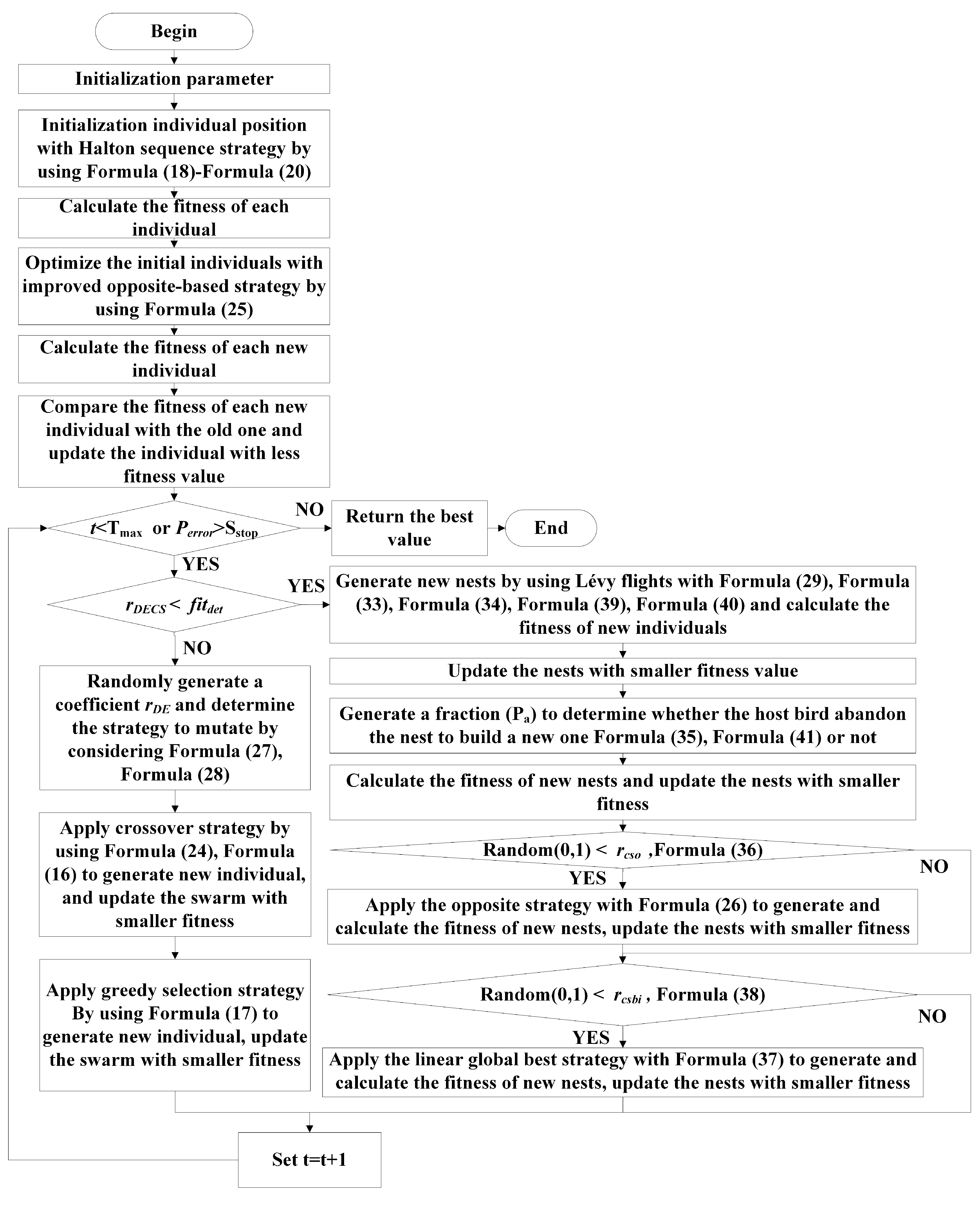
The schematic diagram of the BODE-CS algorithm is shown in Figure 1:

4. Simulation Result and Discussion

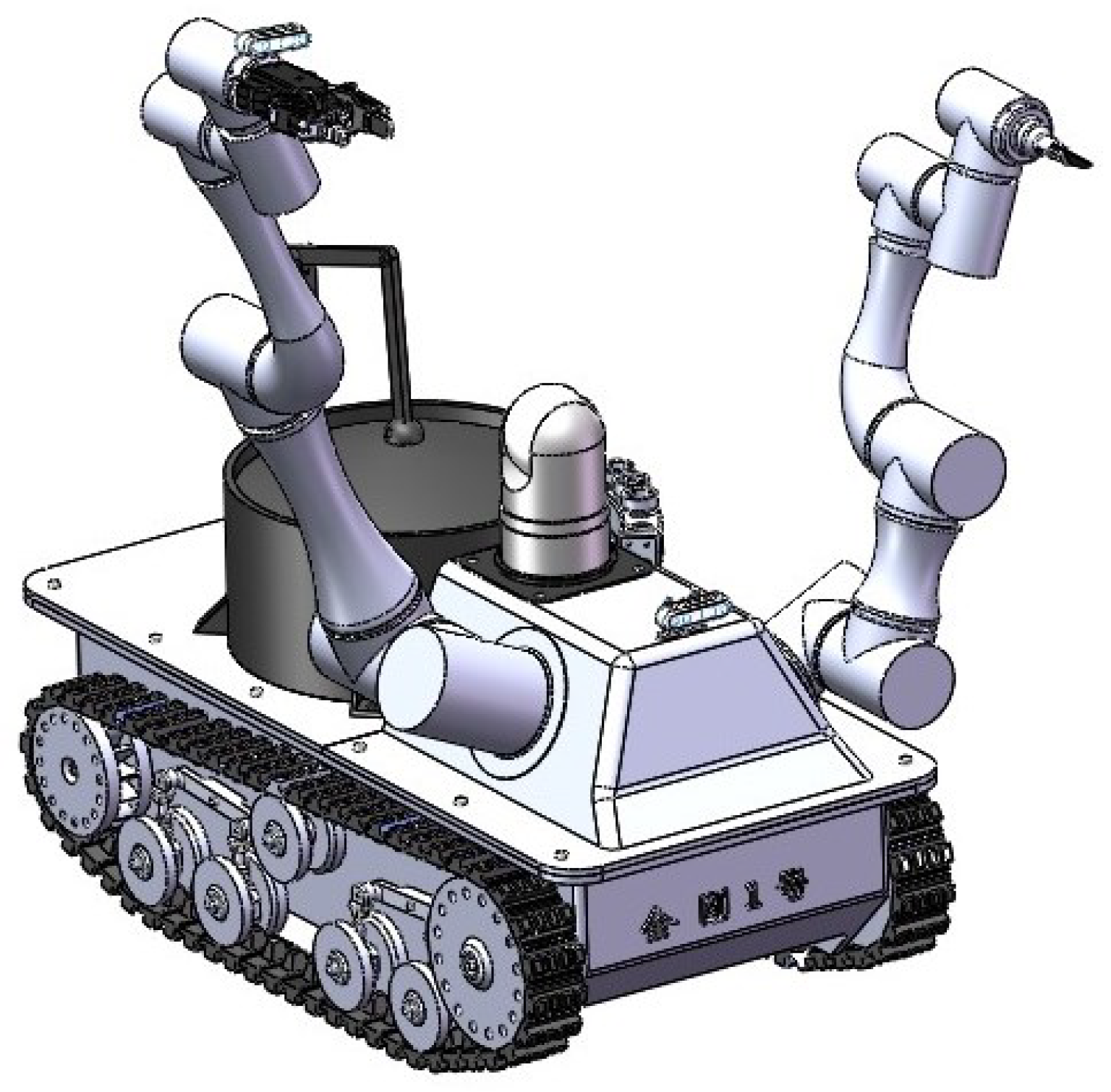
To realize the efficient demolition and rapid disposal of explosives, our team developed a new EOD robot, as shown in Figure 2. It consists of two systems: one is the main mechanical arm system (the left arm, with claw), and the other is the auxiliary mechanical arm system (the right arm, with the cutting tool).

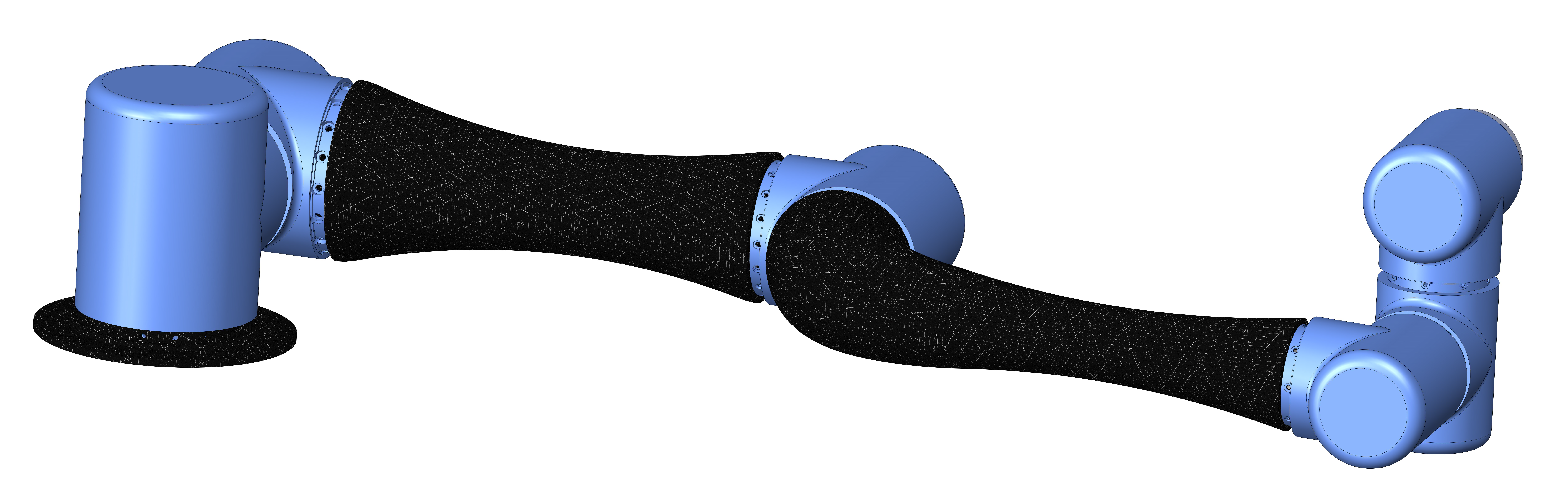
The main manipulator has 6-DOF, which were used to capture and dispose of explosives, and the auxiliary manipulator has six degrees of freedom, which were used to disassemble explosives, as well as assist the main manipulator in observing and defusing explosives. In this paper, we selected the main manipulator as the object to analyze the proposed BODE-CS algorithm. The 3D structure diagram is shown in Figure 3.

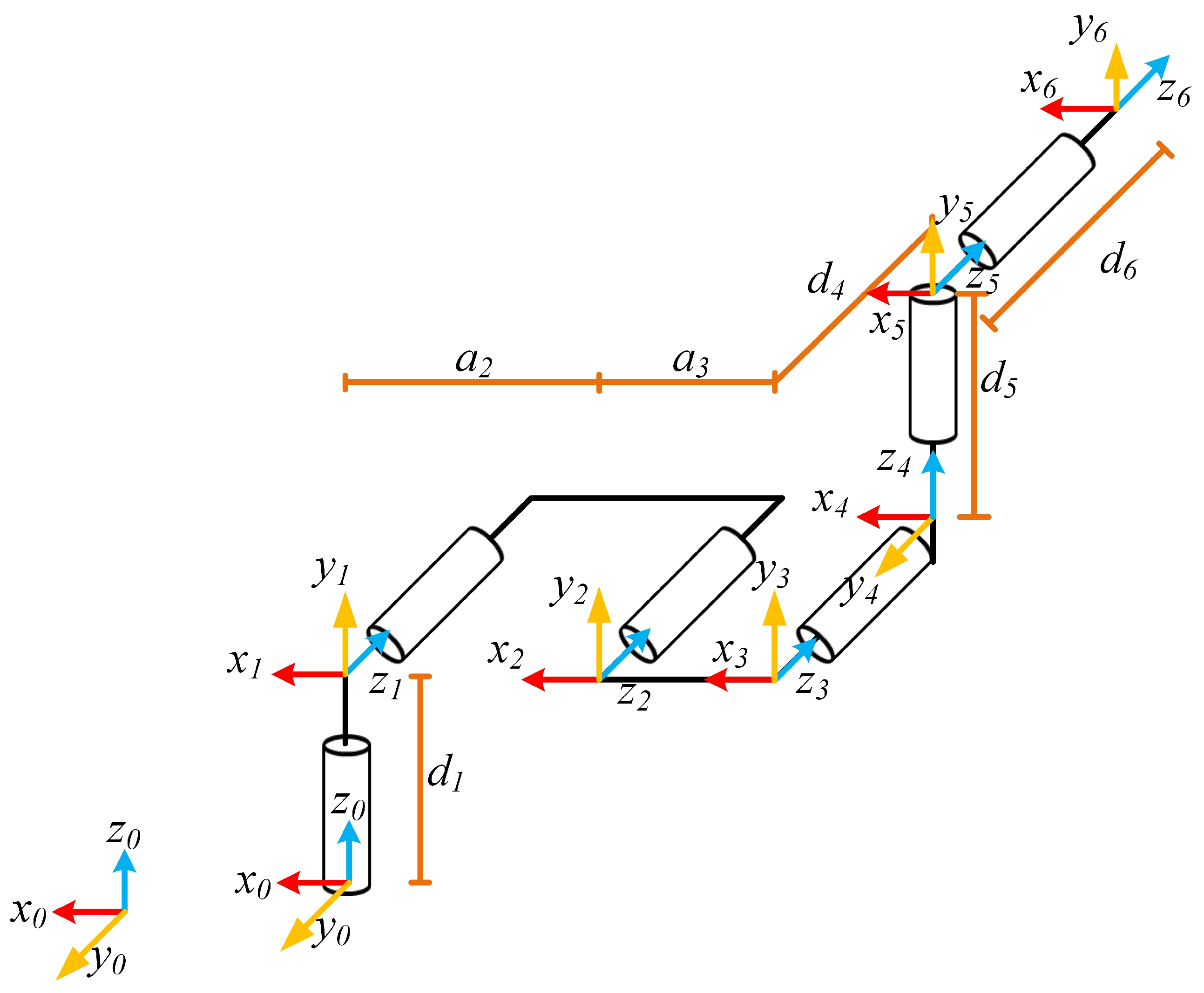
The configuration of the main manipulator is shown in Figure 4:

The D–H parameters are shown in

Table 2. D–H parameter settings for EOD robot manipulator.

i	a (mm)	$\mathit{\alpha }$ (rad)	d (mm)	${\mathit{\theta }}_{\mathit{max}}$ (rad)	${\mathit{\theta }}_{\mathit{min}}$ (rad)
1	0	${\displaystyle \frac{\pi }{2}}$	113.5	${\displaystyle \frac{\pi }{2}}$	$-{\displaystyle \frac{\pi }{2}}$
2	−425	0	0	${\displaystyle \frac{\pi }{2}}$	$-{\displaystyle \frac{\pi }{2}}$
3	−374.9	0	0	${\displaystyle \frac{\pi }{2}}$	$-{\displaystyle \frac{\pi }{2}}$
4	0	$-{\displaystyle \frac{\pi }{2}}$	92.8	${\displaystyle \frac{\pi }{2}}$	$-{\displaystyle \frac{\pi }{2}}$
5	0	${\displaystyle \frac{\pi }{2}}$	110.3	${\displaystyle \frac{\pi }{2}}$	$-{\displaystyle \frac{\pi }{2}}$
6	0	0	56.8	${\displaystyle \frac{\pi }{2}}$	$-{\displaystyle \frac{\pi }{2}}$

:

In Table 2, the parameters a, $\alpha$, d, and $\mathit{\theta }$ represent link length, link twist angle, link offset, and joint angle, respectively.

The main idea involved in BODE-CS algorithms for solving inverse kinematics is to transform the problem to minimize a fitness function, so the final solution is only one. To validate the performance of the BODE-CS algorithm, two simulation experiments were designed: a random-points task and a trajectory-tracking task. The random-points task generated 100 random points and solved the IK problem according to these points. The trajectory-tracking task tracked the respective trajectories of four different curves. The specifications of the test machine were an Intel(R) Core(TM) i5-7500 CPU 3.40 GHz with 8.0 GB of RAM.

4.1. Parameter Setting

The aim of the simulations was to verify the performance of the BODE-CS algorithm to solve the IK problem. In the simulated experiment, several comparative experiments were designed to compare the performance among the BODE-CS algorithm, DE/rand/1 (Standard DE), DE/best/1, DE/rand/2, DE/best/2, DE/current–best/1, SDE [56], CS (Standard CS), PSO, GA, and ODE. A swarm size is typically 5–10 times the population dimension. The dimension of our robot manipulator was six, so we defined the swarm size of all the algorithms as 30. In this study, the robot’s manipulator position accuracy could reach ${10}^{-1}$ mm, so we defined the stop criterion as $S_{\mathit{stop}}=1\times {10}^{-6}$ mm. This criterion could not only compare the position accuracy of different algorithms, but could also meet the position accuracy requirements of robots. Based on the experience of scholars who have studied DE, CS, and other algorithms, we defined the maximum iteration number $T_{\mathit{max}}$ of all the algorithms as 100. The parameters of the BODE-CS algorithm were ${\alpha }_l$ = 0.01, $\beta$ = 3/2, and ${\omega }_P=1$. With many comparative experiments, when we selected $\lambda$ = 0.1, $F_{\mathit{max}}$ = 0.9, $F_{\mathit{min}}$ = 0.5, $w_j$ = 0.7, $w_{\mathit{gbest}}$ = 0.3, $C_{\mathit{max}}$ = 0.8, $C_{\mathit{min}}$ = 0.5, $C_0$ = 0.2, $C_{\mathit{bi}}$ = 0.15, $C_{\mathit{csor}}$ = 0.05, $P_{\mathit{amax}}=0.25$, and $P_{\mathit{amin}}=0.05$, the BODE-CS algorithm showed better performance. Similarly, based on the experience of other scholars, we defined the factor F and $C_R$ in DE/rand/1, DE/rand/2, DE/best/1, DE/best/2, DE/current–best/1, SDE, and ODE, as 0.9 and 0.5, respectively; the factor $\lambda$ in DE/rand/2, DE/best/2, and DE/current–best/1 was defined as 0.1.

The other algorithms’ parameter settings are shown in

Table 3. The parameter setting of CS, PSO, and GA.

Algorithm	Parameter Setting
CS	$P_a$ = 0.25, ${\alpha }_l$ = 0.01, ${\alpha }_g$ = 1, $\beta$ = 3/2
PSO	$c_1$ = 1.2; $c_2$ = 1.2;
GA	$P_m$ = 0.2, $P_c$ = 0.4,

.

The $c_1$ and $c_2$ values represent the acceleration constant; $P_m$ represents mutation probability; and $P_c$ represents the crossover probability.

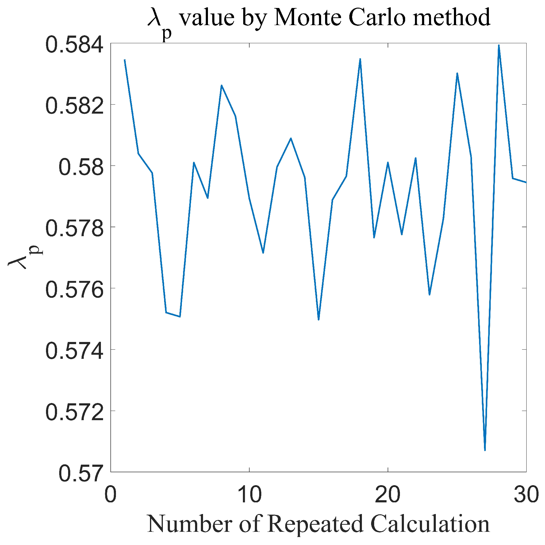
Before obtaining the coefficient ${\omega }_R$ of the BODE algorithm, we used the Monte Carlo method to calculate the ${\mathit{pos}}_{max}$ and ${\mathit{pos}}_{min}$ and obtain ${\lambda }_p$, where 300,000 random points were selected in the workspace to calculate ${\mathit{pos}}_{max}$ and ${\mathit{pos}}_{min}$. Then, we calculated the ${\lambda }_p$ for a total of 30 independent times, the results are shown as follows:

Due to the ${\mathit{pos}}_{\mathit{max}}$ and ${\mathit{pos}}_{\mathit{min}}$ being affected by ${\mathit{l}}_{\mathit{arm}}$, when calculating ${\lambda }_P$ using Formula (10), the difference between ${\mathit{pos}}_{\mathit{max}}$ and ${\mathit{pos}}_{\mathit{min}}$ divided by ${\mathit{l}}_{\mathit{arm}}$. After that, when calculating ${\omega }_R$, ${\lambda }_R$ also divided by the sum of the difference between joint angle upper boundary and joint angle lower bounday in each dimension. As shown in Figure 5, the value of ${\lambda }_p$ approximated to ranges from 0.5725 to 0.5848. To reduce the increase in computational time caused by high-precision decimals, in this paper, we defined ${\lambda }_p=0.58$.

4.2. Task Description

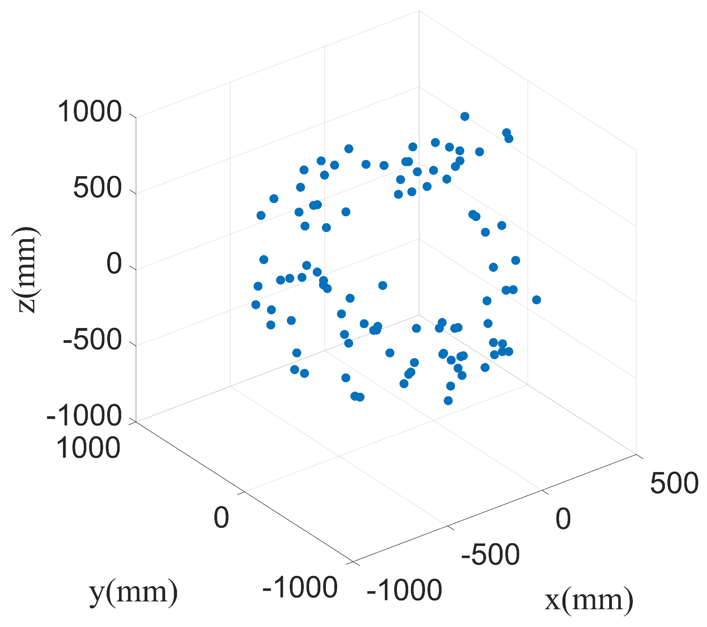
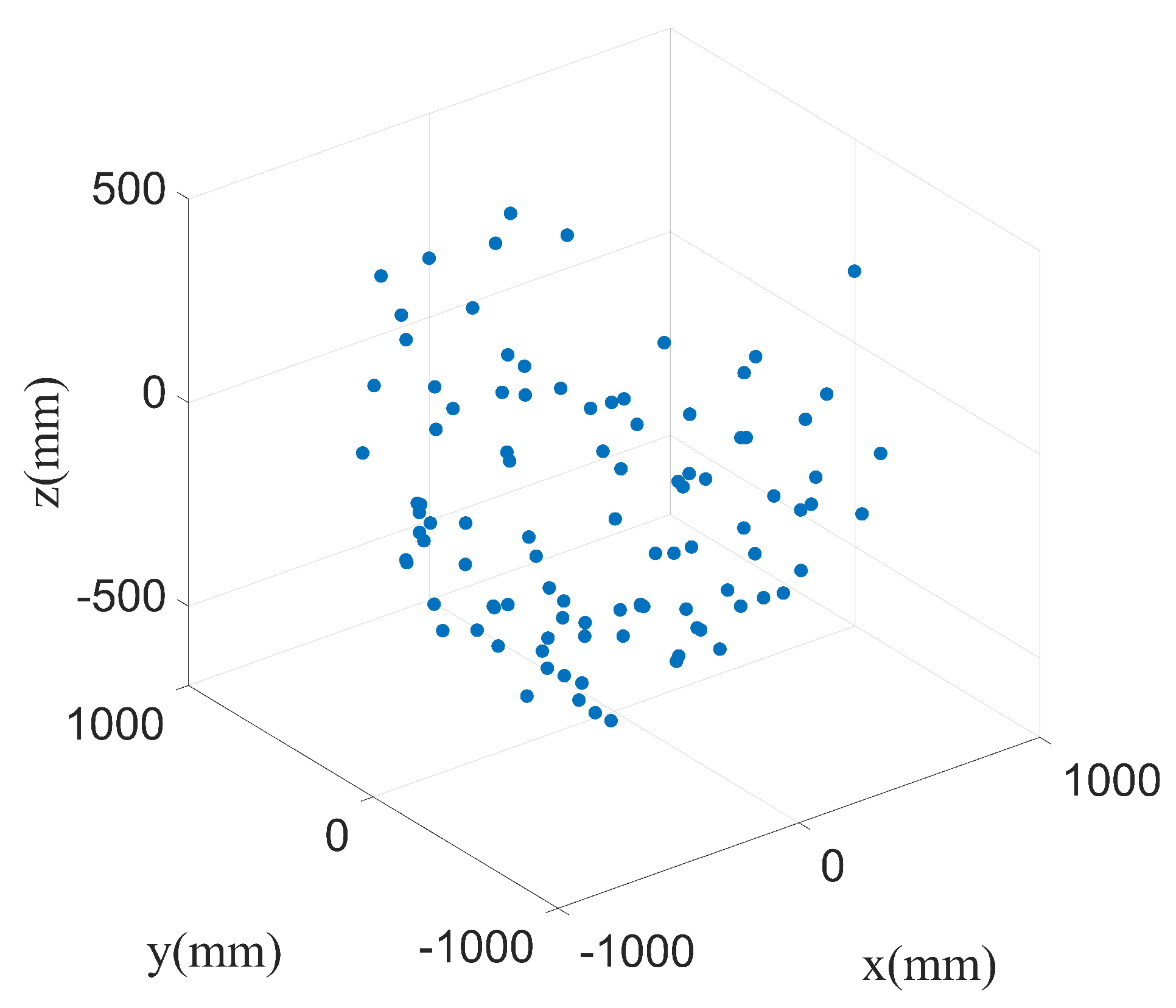
For Task 1, 100 randomly selected points were given, as shown in Figure 6. To ensure the desired random points were generated in the workspace, we used the Monte Carlo method to generate the random points. A comparative study of the IK problem of the random points was conducted. The position and the orientation of all the points were different. The influence of the different weight coefficients on the objective function was first tested; then, the fitness value $\mathit{f}$ and position error ${\mathit{P}}_{\mathit{error}}$ were reported. Finally, the iterative processes of the different algorithms were also evaluated.

For Task 2, the trajectory-tracking simulation was conducted. In this task, we used sinusoidal, circular, trapezoidal, and rose curves to analyze the BODE-CS algorithm. The formulas of the four curves are shown in Formulas (43)–(46), the unit of the four curves is in mm. The main testing included the fitness value $\mathit{f}$, the position error ${\mathit{P}}_{\mathit{error}}$, and so on. To display the statistical variation results of the simulation, a box plot was also used.

Trajectory 1: Sinusoidal

$$\begin{array}{c}{\mathit{p}}_{\mathit{x}}=-500\hfill \\ {\mathit{p}}_{\mathit{y}}\in [-520,-520+300\pi ]\hfill \\ {\mathit{p}}_{\mathit{z}}=-100+400\mathit{sin}\left(\frac{\pi }{150}{\mathit{p}}_{\mathit{y}}\right)\hfill \end{array}$$

(43)

Trajectory 2: Circular

$$\begin{array}{c}\begin{array}{c}{\theta }_p\in [0,2\pi ]\hfill \\ p_x=-500\hfill \end{array}\hfill \\ p_y=-200+300\mathit{sin}\left({\theta }_p\right)\hfill \\ p_z=-100+300\mathit{cos}\left({\theta }_p\right)\hfill \end{array}$$

(44)

Trajectory 3: Trapezoidal

$$\begin{array}{c}{p}_x=500\hfill \\ p_y\in [-520,-100]\hfill \\ r_p=-200+400\sin \left(\frac{\pi }{60}{p}_y\right)\hfill \\ p_z=\left\{\begin{array}{c}0\mathit{if}{r}_p>0\\ -400\mathit{if}{r}_p<-400\\ r_p\mathit{otherwise}\end{array}\right.\hfill \end{array}$$

(45)

Trajectory 4: Rose curve

$$\begin{array}{c}{p}_x=-500\hfill \\ \begin{array}{c}{\beta }_p\in [0,\pi ]\hfill \end{array}\hfill \\ r_p=300\mathit{cos}\left(3{\beta }_p\right)\hfill \\ p_y=-520+r_p\cos \left({\beta }_p\right)\hfill \\ p_z=r_p\sin \left({\beta }_p\right)\hfill \end{array}$$

(46)

The desired orientation matrix matrix of all the trajectories resulted in the following:

$$\mathbf{Rot}=\left[\begin{array}{ccc}0.2838\hfill & \phantom{-}0.8639\hfill & -0.4161\hfill \\ 0.6716\hfill & \phantom{-}0.1307\hfill & \phantom{-}0.7293\hfill \\ 0.6844\hfill & -0.4865\hfill & \phantom{-}0.5431\hfill \end{array}\right]$$

(47)

4.3. Simulation Results for the Robot IK Problem

4.3.1. Results Obtained for Task 1

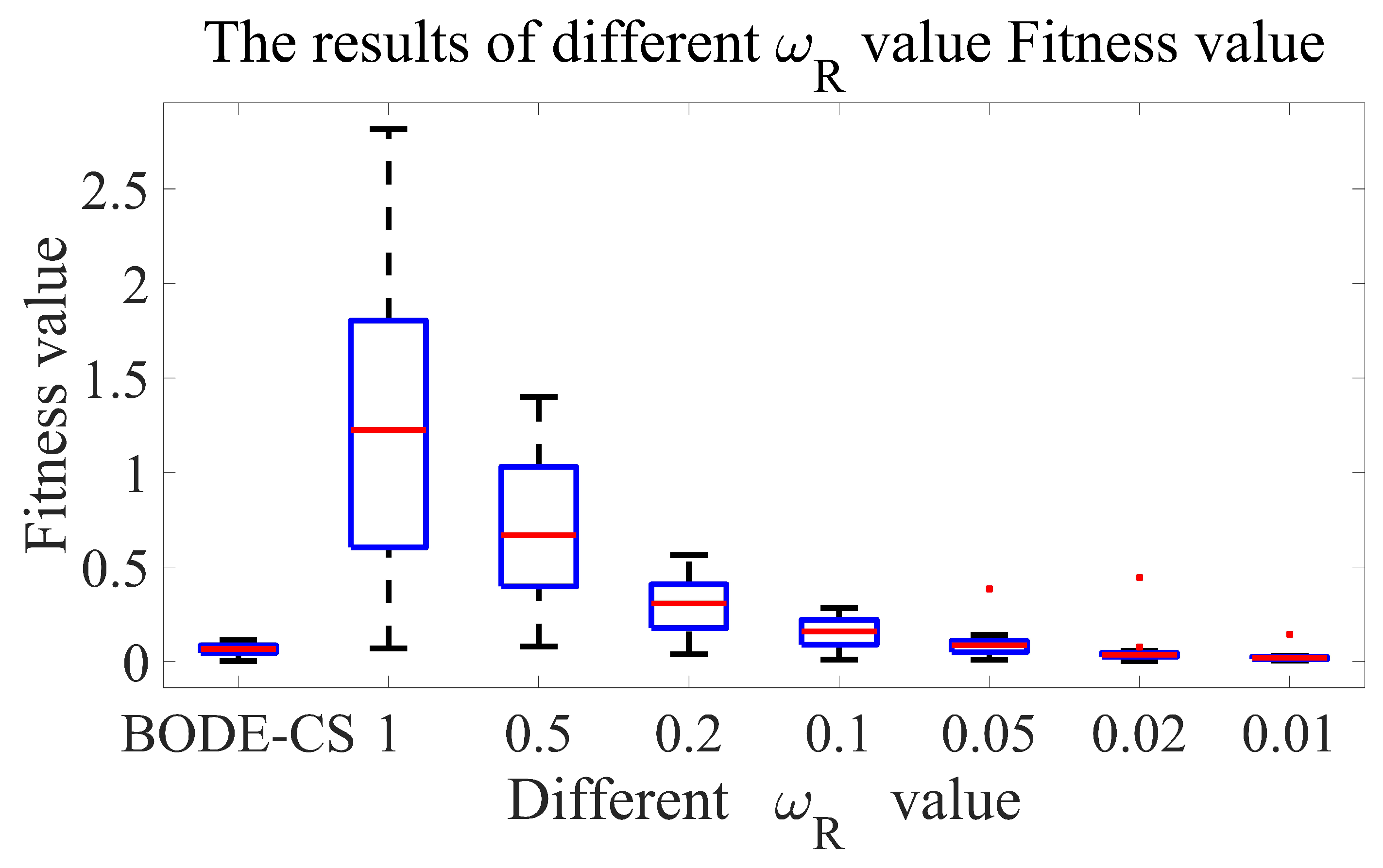
Task 1 aimed to verify the performance of the proposed fitness function (Formula (6)). Several different coefficients were compared, and the results are shown in Figure 7.

To graphically display the statistical variation for the results, box plots were used. The smaller data distribution the algorithm shows, the better performance will be. The BODE-CS represents the weight coefficient of the proposed weight calculation method. As shown in Figure 7, when equipped with the proposed weight method, the fitness of the manipulator could guide the search of the algorithm to converge efficiently. An extensive performance comparison with seven weight coefficients indicates that the proposed BODE-CS reported small data distribution errors and showed the best performance among the eight weight coefficients. The results of the BODE-CS algorithm were precise, with a maximum value of fitness of 0.112. ${\omega }_R$ was related to ${\lambda }_P$, ${\lambda }_R$ and ${\theta }_{\mathit{imax}}$, ${\theta }_{\mathit{imin}}$; ${\lambda }_P$ was related to ${\mathit{pos}}_{\mathit{max}}$, ${\mathit{pos}}_{\mathit{min}}$ and ${\mathit{l}}_{\mathit{arm}}$; ${\lambda }_R$ was related to ${\lambda }_P$; and ${\mathit{l}}_{\mathit{arm}}$ was related to $d_i$ and $a_i$. Thus, ${\omega }_R$ was related to the robot structural parameters. The fitness value calculated by the proposed weight method (Formulas (6)–(12)) was smaller for the optimized coefficients when considering the robot structural parameters.

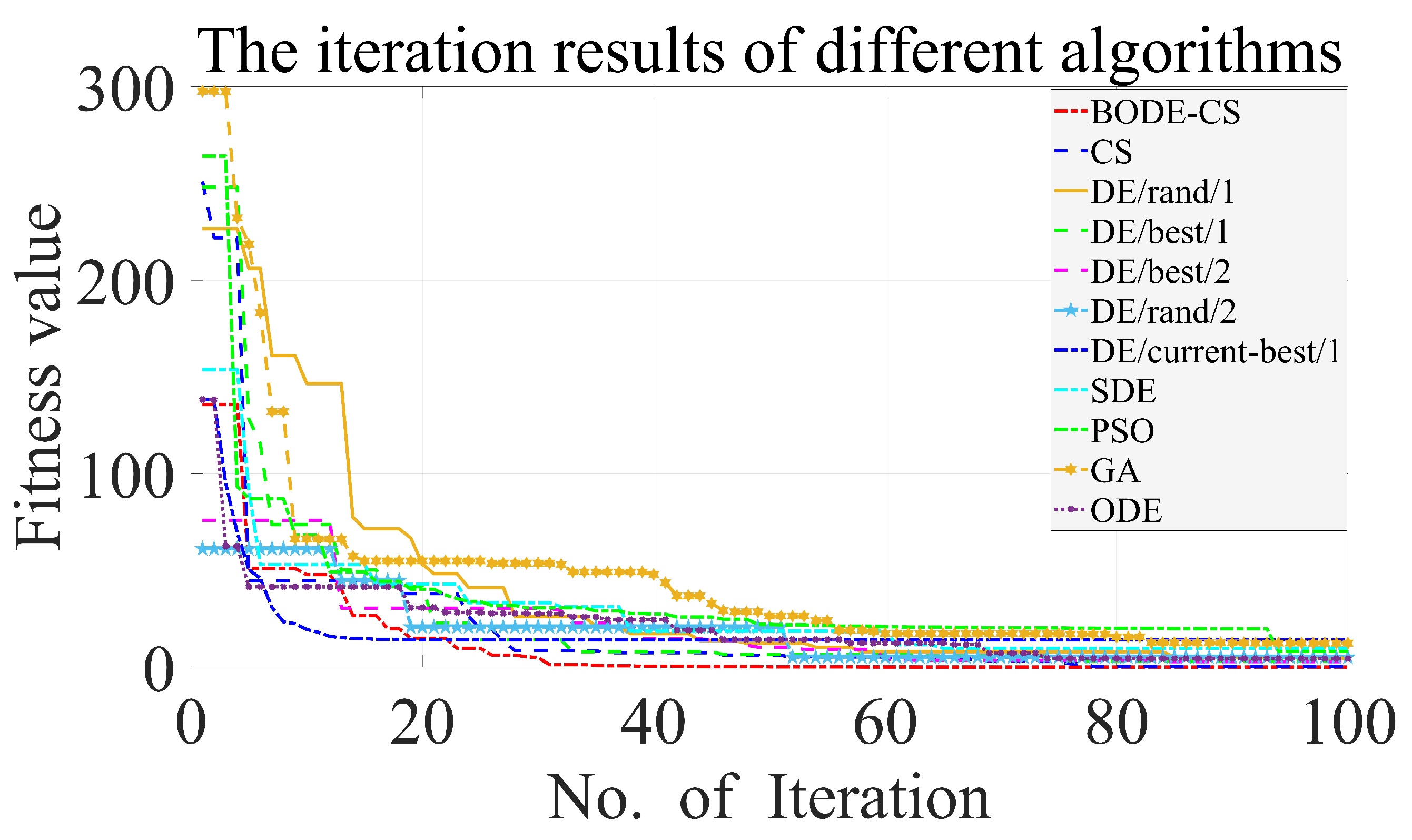
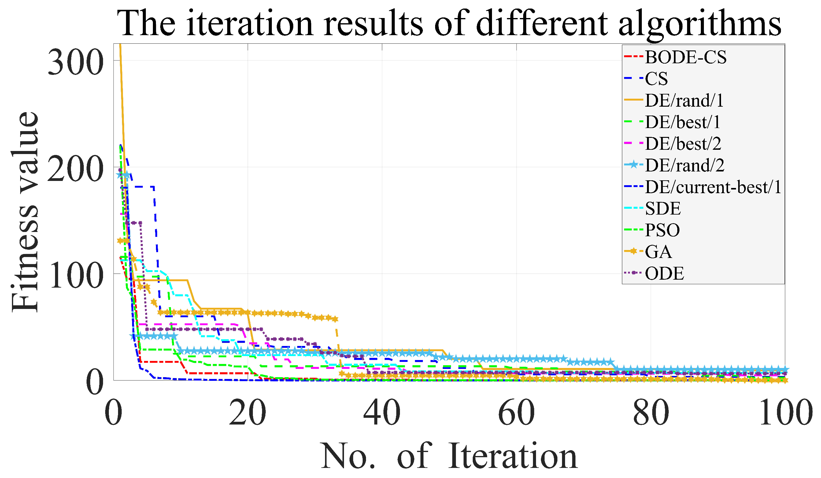
Additionally, to verify the performance of proposed strategies in the BODE-CS algorithm, we compared the ${\mathit{k}}_{\mathit{th}}$ point iteration process of the BODE-CS algorithm with other algorithms. Figure 8 shows the iteration results for the inverse kinematics problem of 100 random points. The reported results indicate that the proposed BODE-CS algorithm could balance the global search with the local search and outperformed the other algorithms, with a minimum fitness value of 0.0833. The second-lowest minimum fitness value among the other 10 algorithms was 0.3868 (CS). The DE/best-best/1 strategy made the BODE-CS algorithm have a fast convergence rate and better results; when the iteration number reached 63, the fitness value was less than 0.1. The BODE-CS algorithm showed faster convergence than the other algorithms.

Two parameters were used to compare the stability of the algorithms–the maximum fitness value and maximum position errors. The maximum position error and the maximum fitness value represented the maximum position error and the maximum fitness value of all the 100 random points, respectively. The results for solving the IK problem of 100 random points are illustrated in

Table 4. Inverse kinematics with 100 random points using different algorithms.

Algorithm	Maximum Position Error (mm)	Maximum Fitness Value
BODE-CS	0.070	0.112
DE/rand/1	13.484	13.552
DE/best/1	6.770	6.874
DE/best/2	11.466	11.466
DE/rand/2	12.939	12.939
DE/current-best/1	129.239	129.253
SDE [56]	15.359	15.385
CS	10.897	10.898
PSO	14.963	15.213
GA	78.271	78.377
ODE	16.694	16.705

. The introduction of the algorithm selection function streamlined the balance between the global and local searches. As shown in Table 4, the BODE-CS had the best performance, with the lowest fitness value and position errors of all the algorithms.

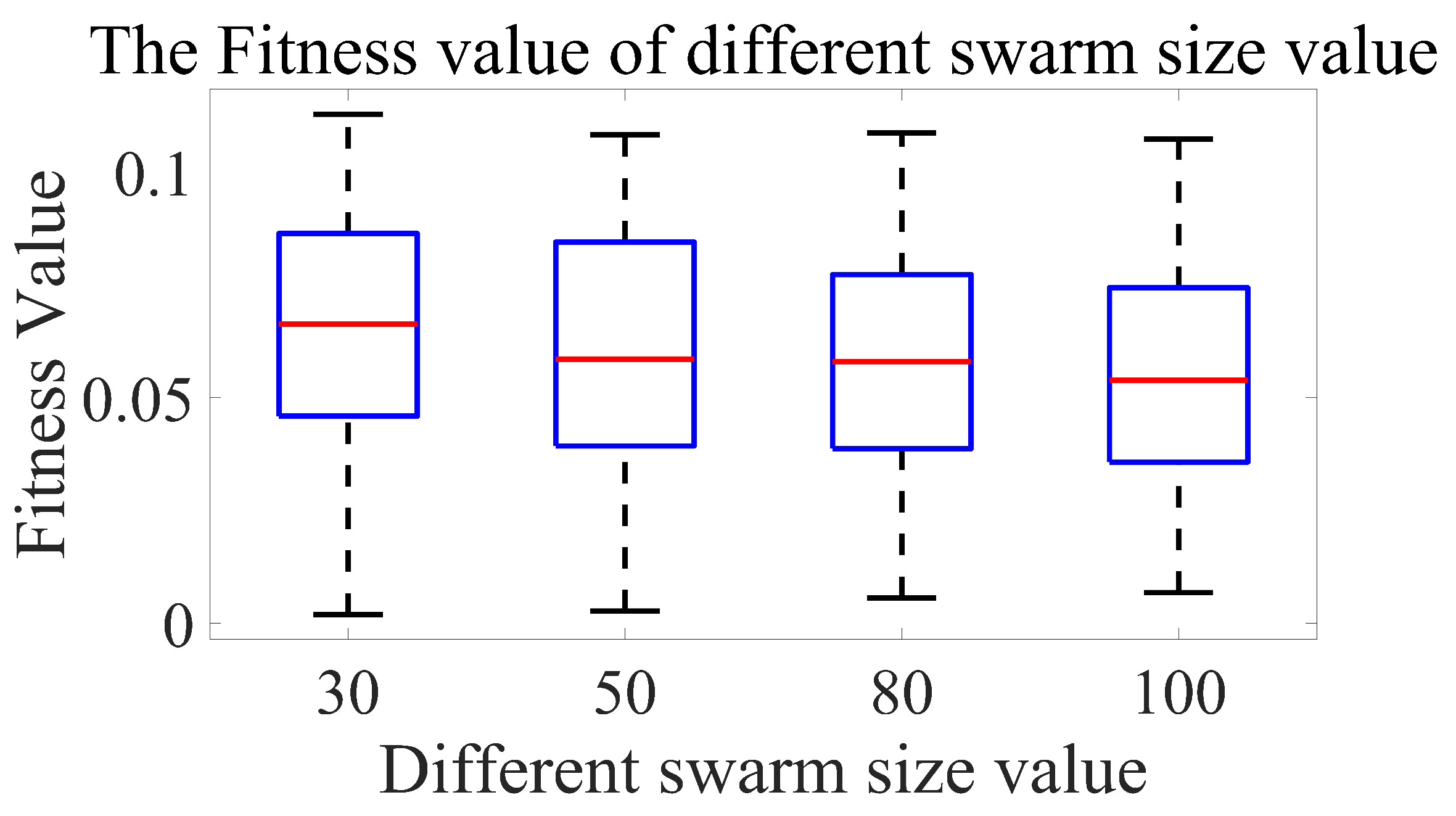
To verify the influence of swarm size on the convergence results, four different-sized swarms were selected; the swarm sizes were 30, 50, 80, and 100; the ${\mathit{S}}_{\mathit{stop}}={10}^{-20}$ mm, and the results are shown in Figure 9.

As shown in Figure 9, with the increases in swarm size, the maximum fitness values of the iterations were always less than 0.15; the results for 30 individuals were similar to the other numbers of the individuals. The precision requirements for the explosive removal were not very high when the number of the trajectory or random points was less than 100. The smaller the swarm size was, the shorter the calculation time would be, so the swarm size selected in this study was appropriate.

Generally, the Jacobian-based method has the advantage of fast convergence and high precision; to verify the performance of the BODE-CS algorithm, we also compared the BODE-CS algorithm with the Newton–Raphson algorithm (Jacobian-based method). The initial solution of Newton–Raphson was set to [0 0 0 0 0 0]; the stop criterion of Newton–Raphson was equal to the BODE-CS algorithm. The comparison results of Newton–Raphson and the BODE-CS algorithm were shown ains

Table 5. The comparison results of Newton–Raphson and BODE-CS in solving 100 random-points task.

Algorithm	Position Error (mm)			Fitness Value
	Min	Mean	Max	Min	Mean	Max
BODE-CS	$7.184\times {10}^{-6}$	$5.895\times {10}^{-4}$	0.0070	$9.690\times {10}^{-3}$	$6.707\times {10}^{-2}$	0.112
Newton-Raphson	$2.842\times {10}^{-14}$	57.150	1427.9	$2.843\times {10}^{-14}$	57.151	1427.9

:

The results show that, compared with the Newton–Raphson algorithm, the BODE-CS algorithm performed better, with a smaller mean or maximum position error, as well as mean or maximum fitness value. The Newton–Raphson algorithm showed a better minimum position error and fitness value. The precision of the Newton–Raphson algorithm was high; however, the solutions calculated by the Newton–Raphson algorithm were not stable. This is because of the influence of singular configuration and initial solution setting. In most situations, the precision of the Newton–Raphson algorithm is high; however, with the influence of singular configuration or initial solution setting, the result was difficult to converge. Thus, in general, the performance of the BODE-CS algorithm was better than Newton–Raphson.

In many situations, the EOD robot did not require high orientation accuracy when grabbing or defusing explosives. Thus, we designed another 100 random-points trjaectory task, which only considered the position requirements (${\omega }_P=1$, ${\omega }_R=0$ in Formula (6)) to verify the applicability of the proposed algorithm in solving different tasks. The $\mathit{k}$th random point iteration process for different algorithms is shown below.

As shown in Figure 10, the proposed BODE-CS algorithm also outperformed the other algorithms. The algorithm selection function and other improved strategies kept the diversity and accelerated the swarm convergence, with a minimum fitness value of 0.00012. The second-lowest minimum fitness value among the other algorithms was 0.04316 (GA). When the iteration number reached 46, the fitness value of the BODE-CS algorithm was less than 0.1.

As shown in Formula (6), when ${\omega }_R=0$, the value of fitness is equal to the position error $\mathbf{\Delta }\mathit{P}$. Therefore, we only need to compare the maximum fitness value to select the best algorithm. As shown in

Table 6. Inverse kinematics with 100 random points using different algorithms (position requirement).

Algorithm	Maximum Fitness Value
BODE-CS	0.0075
DE/rand/1	15.9222
DE/best/1	9.0836
DE/best/2	7.8957
DE/rand/2	14.5838
DE/current-best/1	161.2696
SDE	15.5102
CS	12.461
PSO	52.8607
GA	110.2148
ODE	18.4566

, with the introduction of the improved Lévy flight strategy and the DE/best-best/1 strategy, the proposed algorithm could balance the global search and local search. The premature phenomenon could also be avoided. The simulation results of the BODE-CS strategies showed the best performance. The maximum fitness value of BODE-CS algorithm was 0.0075. It was also the smallest of all the algorithms.

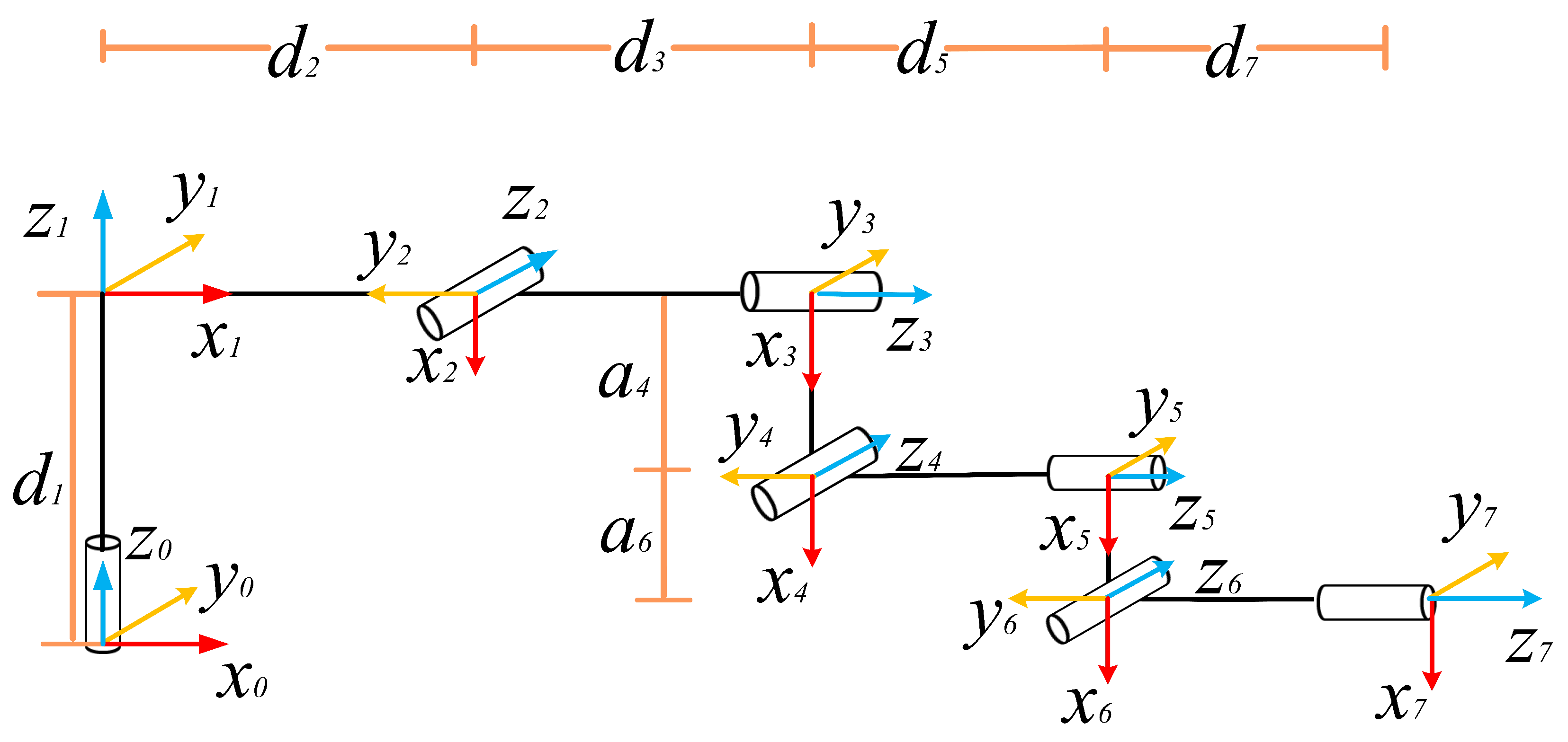
To further verify the applicability of the BODE-CS algorithm, we introduced a 7-DOF Baxter redundant manipulator and solved its inverse kinematics problem of 100 random points. The coordinate system of link i, D–H parameters, and the distribution of 100 random points are shown in Figure 11,

Table 7. Baxter’s Denavit–Hartenberg parameters.

i	a (mm)	$\mathit{\alpha }$ (rad)	d (mm)	${\mathit{\theta }}_{\mathit{max}}$ (rad)	${\mathit{\theta }}_{\mathit{min}}$ (rad)
1	0	0	270.35	$\frac{\pi }{2}$	$-\frac{\pi }{2}$
2	0	$-\frac{\pi }{2}$	69	$\frac{\pi }{3}$	$-\frac{\pi }{2}$
3	0	$\frac{\pi }{2}$	364.35	$\frac{\pi }{2}$	$-\frac{\pi }{2}$
4	69	$-\frac{\pi }{2}$	0	$\frac{\pi }{2}$	0
5	0	$\frac{\pi }{2}$	374.29	$\frac{\pi }{2}$	$-\frac{\pi }{2}$
6	10	$-\frac{\pi }{2}$	0	$\frac{\pi }{2}$	$-\frac{\pi }{2}$
7	0	$\frac{\pi }{2}$	229.529	$\frac{\pi }{2}$	$-\frac{\pi }{2}$

, and Figure 12, respectively. Therein, the offset of ${\theta }_2$ is $\pi /2$.

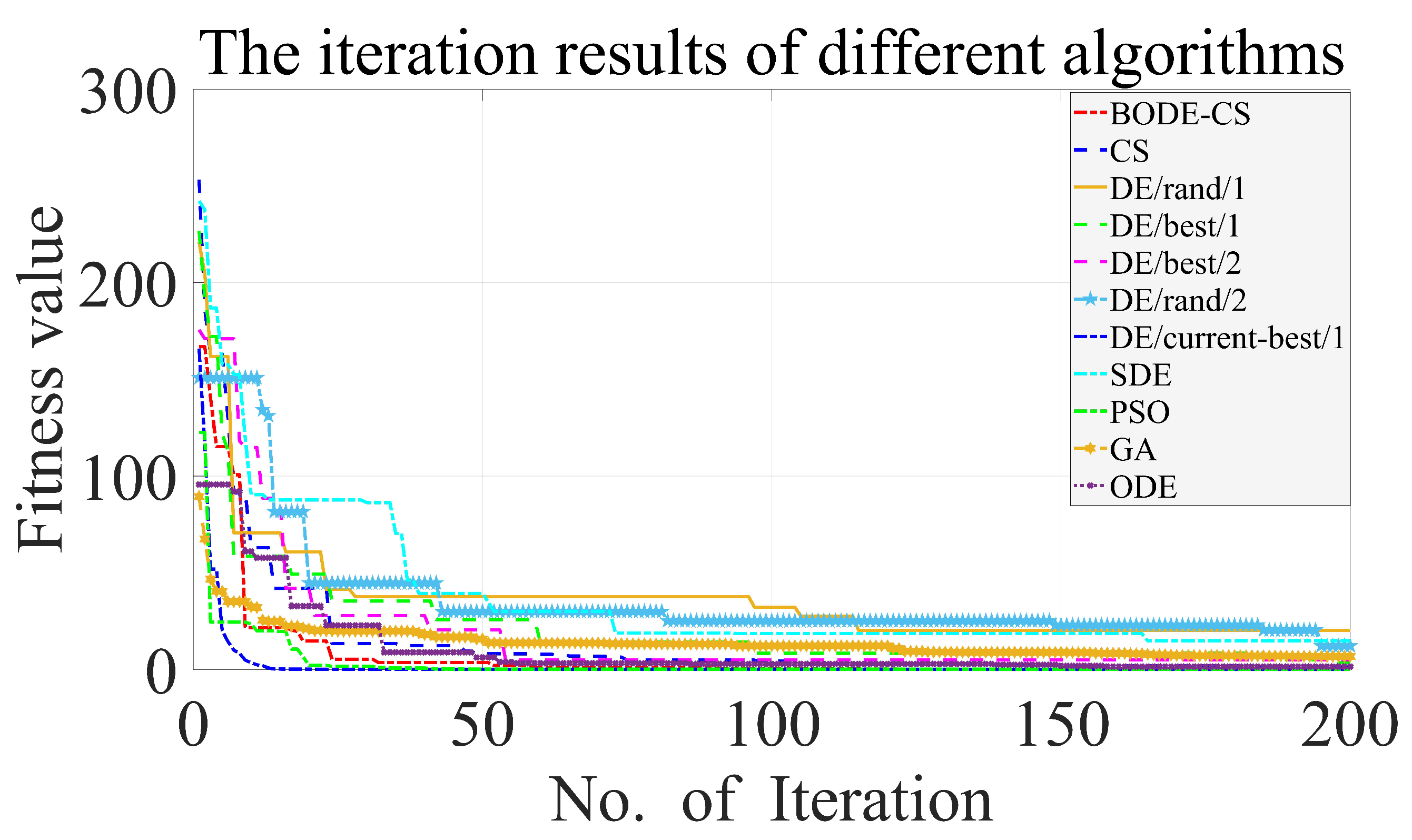
Additionally, to verify the applicability of the BODE-CS algorithm, we compared the iterative process of the BODE-CS algorithm with other algorithms. The maximum iteration number ${\mathit{T}}_{\mathit{max}}$ was 200; the swarm size was 70. Figure 13 shows the iteration results for the inverse kinematics problem of 100 random points. The proposed BODE-CS algorithm outperformed the others, with a minimum fitness value of 0.0572. The second-lowest minimum fitness value among the other 10 algorithms was 0.1265 (DE/current-best/1). The BODE-CS algorithm had a fast convergence, and, when the iteration number reached 164, the fitness value was less than 0.1. The BODE-CS algorithm shows wide applicability and faster convergence than other algorithms.

The maximum fitness value and position error for solving the IK problem of 100 random points are illustrated in

Table 8. Inverse kinematics of a 7-DOF redundant robot manipulator with 100 random points using different algorithms.

	Maximum Position Error (mm)	Maximum Fitness Value
BODE-CS	0.0062	0.1014
DE/rand/1	28.0690	28.14704
DE/best/1	19.9514	20.0162
DE/best/2	23.8813	23.9331
DE/rand/2	20.8778	20.9458
DE/current-best/1	46.3560	46.4510
SDE	24.8601	24.9414
CS	3.1545	3.1707
PSO	36.2566	36.3429
GA	62.0163	62.1044
ODE	21.3118	21.3953

. The maximum position error and maximum fitness value were also used to compare the stability of the algorithms. The introduction of algorithm selection function makes it easy to balance the global search and local search in solving the 7-DOF IK problem. Therein, the BODE-CS algorithm also showed the best performance, with the smallest fitness value and position error in all the algorithms. The applicability of the widely used algorithm is further proved.

4.3.2. Results Obtained for Task 2

In Task 2, to better verify the performance of the BODE-CS algorithm, we selected 200 trajectory points for tracking. Due to the increase in the trajectory points, the calculations were more complex; thus, the probability of higher fitness values or position errors increased. Therefore, we redefined the swarm size as 60. As shown in

Table 9. The results of four curves trajectories tracked using different algorithms.

Algorithm	Trajectory 1		Trajectory 2		Trajectory 3		Trajectory 4
	Maximum Position Error	Maximum Fitness Value	Maximum Position Error	Maximum Fitness Value	Maximum Position Error	Maximum Fitness Value	Maximum Position Error	Maximum Fitness Value
BODE-CS	0.017	0.100	0.016	0.120	0.004	0.110	0.083	0.182
DE/rand/1	7.706	7.713	6.946	6.958	9.254	9.356	8.56	8.635
DE/best/1	4.779	4.832	4.895	4.897	6.446	6.472	4.083	4.155
DE/best/2	4.782	4.784	4.200	4.214	7.785	7.806	4.415	4.425
DE/rand/2	7.303	7.347	7.772	7.790	9.943	9.978	7.384	7.413
DE/current-best/1	43.999	44.009	73.680	73.700	49.421	49.445	54.278	54.322
SDE	11.419	11.439	11.672	11.713	10.025	10.030	9.239	9.299
CS	4.538	4.610	4.649	4.661	4.036	4.139	4.871	4.954
PSO	4.111	4.154	5.203	5.249	2.466	2.535	6.577	6.594
GA	41.721	41.758	48.613	48.656	46.981	47.004	43.831	43.874
ODE	10.543	10.548	10.672	10.740	9.584	9.658	10.163	10.179

, the maximum position errors corresponding to the IK solution of DE/current–best/1 and GA in the four curves were all more than 10 mm. Due to the relatively large maximum position error values, the IK solutions calculated by the two algorithms were unacceptable. Although the IK solutions obtained from the other eight algorithms were smaller, the cumulative error of adjacent points in a trajectory could considerably increase, and the stability of robot motion would be affected. The BODE-CS algorithm obtained the first rank with the minimal maximum position error and maximum fitness values in the four curves, and the maximum position errors of all four curves were less than 0.1 mm. The results show better performance than those of the other 10 algorithms.

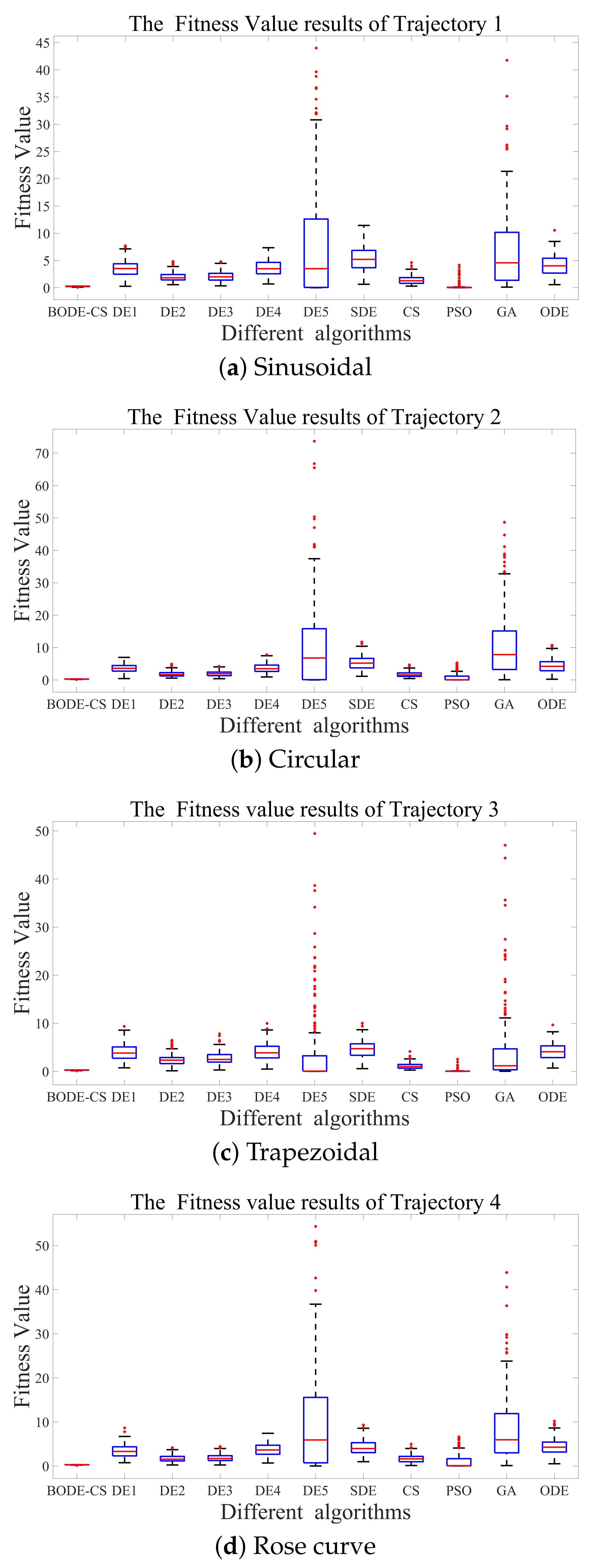
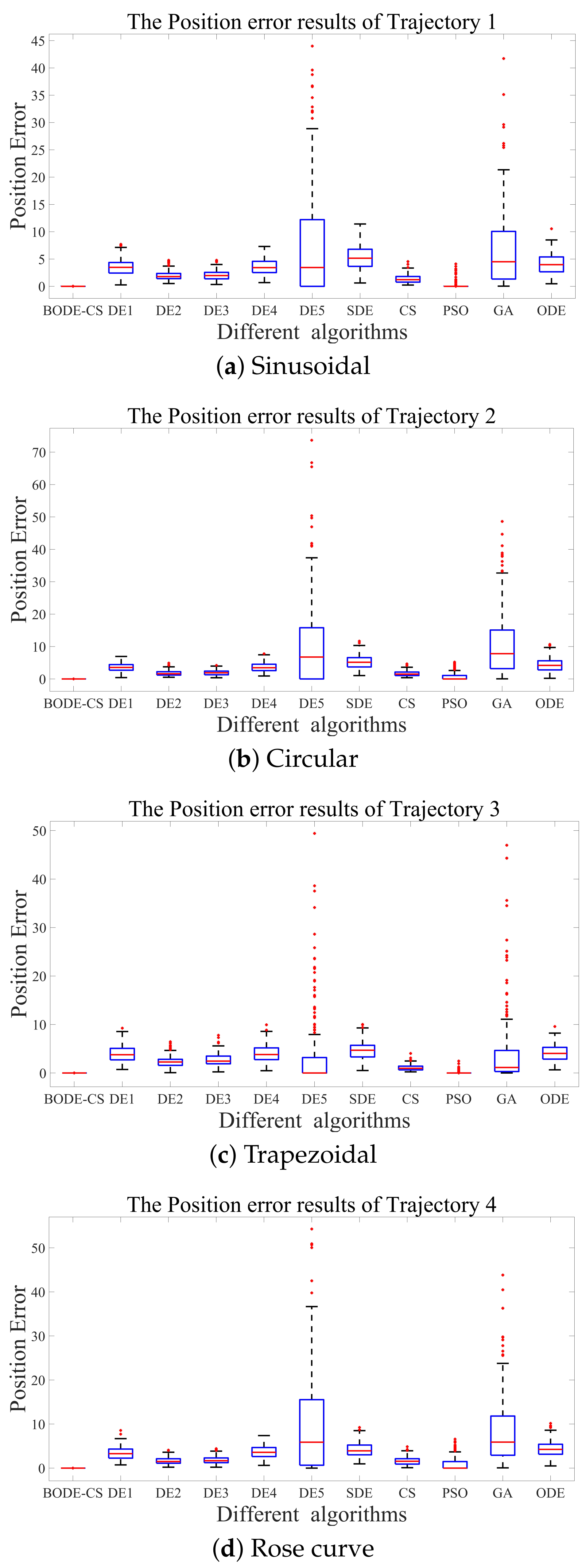
To compare the trajectory-tracking results of all the algorithms in different curves, the fitness and postion distributions of all the algorithms were also analyzed. In Figure 14 and Figure 15, DE1, DE2, DE3, DE4, and DE5 represent DE/rand/1, DE/best/1, DE/best/2, DE/random/2, and DE/current-best/1, respectively. The position error results and fitness value results are displayed graphically. When the ${\omega }_R$ was small, the influence of orientation error times ${\omega }_R$ showed smaller values for the fitness function, so the position error was sometimes almost equal to the fitness value. For example, the results in Figure 14b were similar those in Figure 15b, so the fitness value analysis results were similar to the position error analysis results; thus, we only needed to discuss the analysis results for the position errors.

The position errors of the DE/current–best/1 and GA during the trajectory tracking were distributed over a large range. There are three reasons that may have influenced the results of DE/current–best/1 and GA: small swarm size, the quality of initial individuals, and the influence of the best individual. Due to the small swarm size and poor quality of initial solutions, the convergence of DE/current–best/1 and GA may have been slow, or premature phenomenon; if there are many same local best individuals in the swarm early on, the explore ability will decrease, and the swarm will show poor results. Therefore, the DE/current–best/1 and GA were not suitable for tracking the four trajectories. DE/best/1, DE/rand/1, and the other six algorithms had better performance results than DE/current–best/1 and GA; however, when compared to our proposed algorithm, their stabilities were poor, and the maximum position error was also large. Therefore, the proposed BODE-CS algorithm was the most suitable algorithm for trajectory tracking.

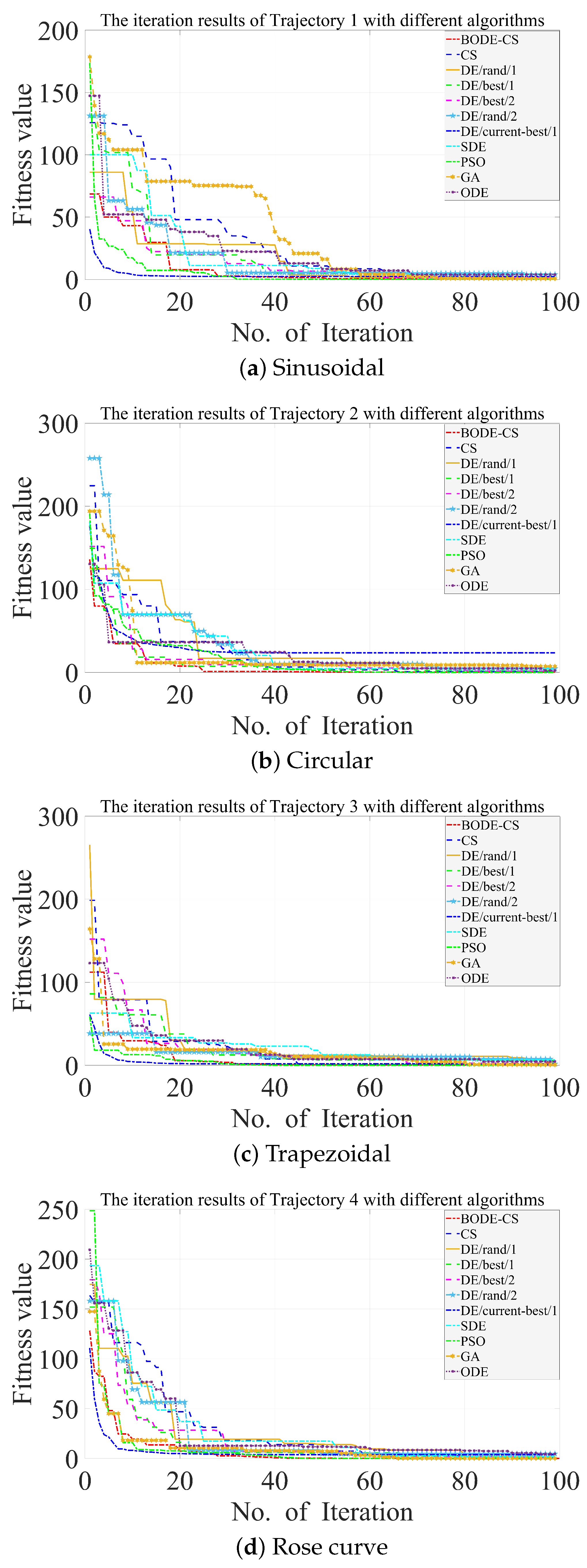
To further verify the trajectory tracking iteration results of the BODE-CS algorithm, we analyzed the iteration results of all the algorithms in four different curves. The results are shown as Figure 16, for all the trajectory iteration results generated by the algorithms, the BODE-CS algorithm acquired the first rank, with the following minimum fitness values: 0.065 (Trajectory 1), 0.059 (Trajectory 2), 0.100 (Trajectory 3), and 0.075 (Trajectory 4). Compared to the other algorithms, the BODE-CS algorithm also showed a rapid convergence rate when the fitness value reached 0.1. The iteration numbers when the fitness value reach 0.1 were 62 (Trajectory 1), 50 (Trajectory 2), 53 (Trajectory 3), and 43 (Trajectory 4). The proposed BODE-CS algorithm showed better convergence than the other algorithms.

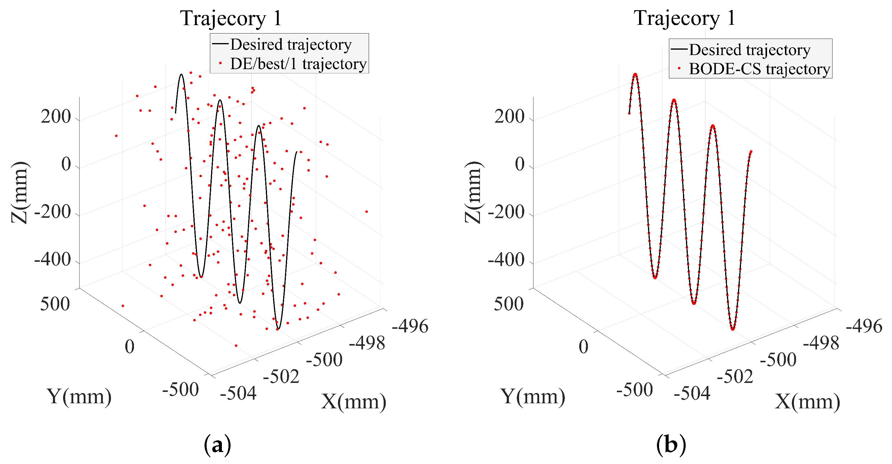
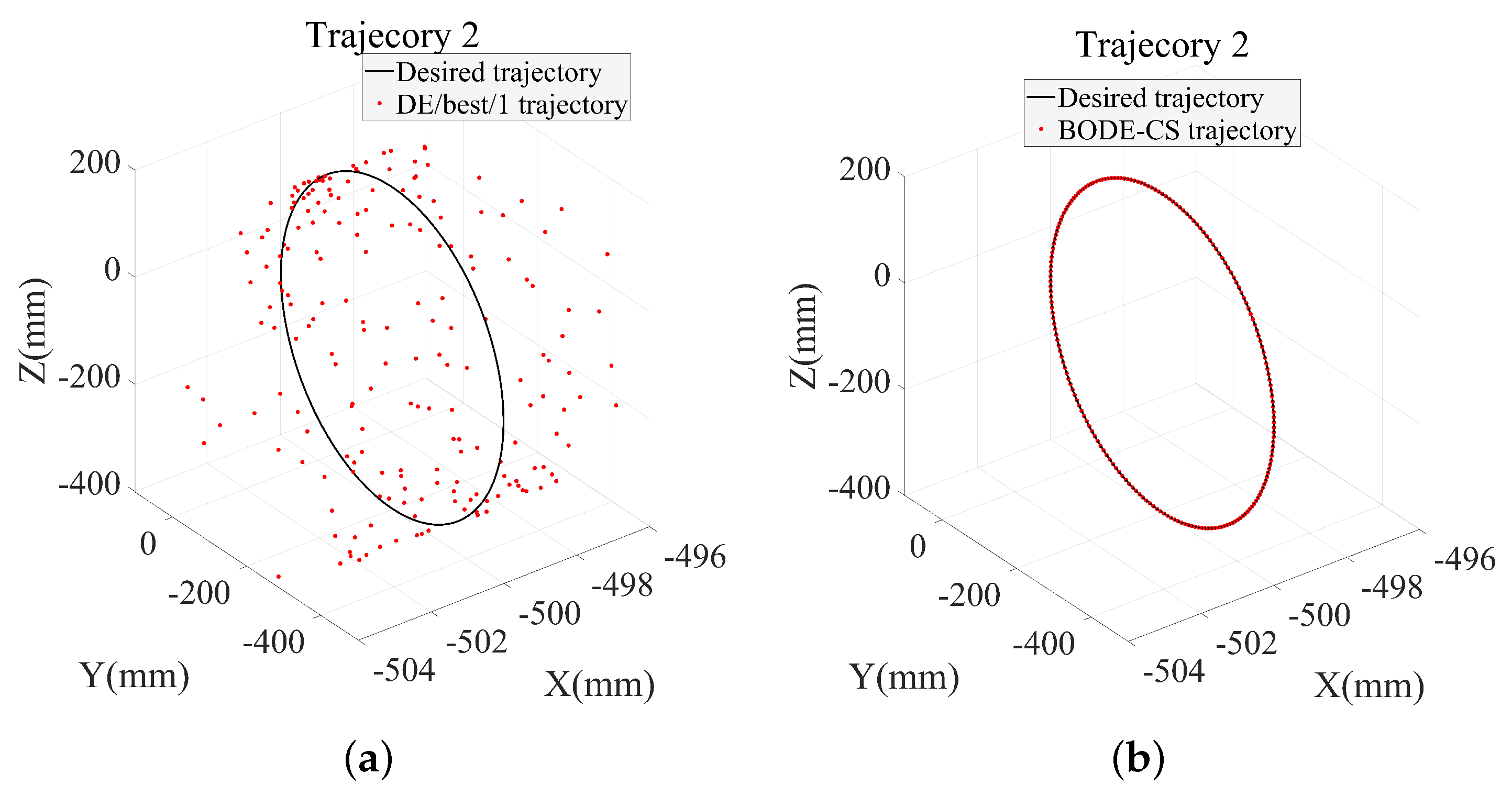
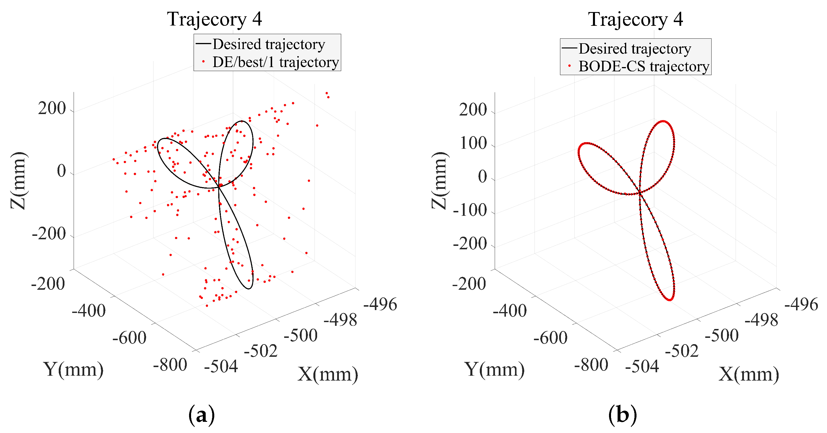
Moreover, Figure 17, Figure 18, Figure 19 and Figure 20 show the Trajectory 1–4 tracking results of the DE/best/1 and BODE-CS algorithm, respectively. The black curve shows the desired trajectory, and the red point shows the calculation results using the DE/best/1 (Figure 17a) or BODE-CS (Figure 17b), respectively. The trajectory results showed that the DE/best/1 method presented a rough motion. The statical variation of the trajectory tracking showed a large data distribution. Compared to the DE/best/1 algorithm, the Lévy flight in the improved CS strategy led the proposed algorithm to search for a new environment, and the consistency of the BODE-CS algorithm showed a minimal data distribution. As compared to the DE/best/1 algorithm, the results indicated that the BODE-CS had more precise and accurate path-tracking results. The desired end-effector position and the obtained position were considered to be identical.

5. Conclusions and Future Developments

In this study, a novel hybrid BODE-CS algorithm was presented to solve the IK problem in robot manipulators. The simulated experiments were designed to verify the performance of our proposed hybrid algorithm for solving a trajectory-tracking problem. There are five contributions in this research. Firstly, a novel fitness function was formulated, which considered the robot’s structural requirements, which included the link length and offset, as well as the joint angle. The Monte Carlo method was also applied to calculate the weight coefficients of the orientation error. Compared to other weight coefficients, the algorithm accuracy was improved efficiently using the proposed novel fitness function. Then, the initial solutions were optimized using a Halton sequence and an opposite strategy to ensure the initial solutions were distributed more evenly in order for the solution quality to be improved. Moreover, multiple strategies were applied for DE and CS. The Lévy flight in the CS algorithm could improve the global search ability, and the limitations of using a single algorithm could be avoided; thus, a new function was designed to choose the proper algorithm. The scale factor F, the cross-over probability factor $C_r$, a dynamically opposite strategy, and a bidirectional strategy were used to optimize the DE algorithm. Additionally, two typical DE algorithms were combined with the proposed strategies to form a novel composite DE algorithm. The CS was optimized with the linear best global strategy and dynamically opposite strategy. These strategies could efficiently enhance the exploration and explosive abilities. Finally, two tasks were designed, and the results showed that the BODE-CS algorithm outperformed the other 10 algorithms when solving the IK problem of 100 random points and for tracking different curve trajectories. The simulations showed that the BODE-CS algorithm showed the best performance of all the algorithms; the reported position error results of the BODE-CS algorithm were below 0.01 mm, with a swarm size of 30 and a maximum iteration of 100. The convergence rate was also superior to other algorithms when solving the 100 random-points task and the trajectory-tracking task. The results of the BODE-CS algorithm also showed consistent statistical results with minimal data distribution. Meanwhile, the applicability was also verified with a different fitness function, a 7 DOFs robot, and compared with Jacobian-based algorithm, respectively. The convergence rate and result also outperformed all the other algorithms.

However, although the proposed BODE-CS algorithm showed the better performance in solving the IK problem and trajectory tracking problem, there may be several limitions in this study. Firstly, we optimized the traditional DE algorithm with multiple strategies. Therefore, more control parameters were introduced; although the proposed algorithm showed better performance when solving the low dimensional problem (6 or 7 DOF robots), it may spend a lot of time to set the proper parameters when solving high dimensional (15 or more) problem. Secondly, more time was consumed by using the proposed algorithm to calculate the fitness value. The mean calculation time of the BODE-CS algorithm in Task 1 (${\mathit{T}}_{\mathit{max}}$ = 100, N = 30, repeat the calculation 30 times) was 7.96 s; the maximum mean calculation time of the other algorithms was 7.25 s (Cuckoo Search). Thirdly, when solving the trajectory tracking problem, we ignored the obstacle avoidance analysis. It was also an important issue when solving the trajectory-tracking problem in complex environments. Finally, the desired points in this paper were all in the workspace. If the desired point is not in the workspace, the motion of the mobile platform should be considered. Future research should design a strategy to balance the time consumption, and algorithm accuracy. The study should also focus on theoretical guidelines for selecting the proper parameter in the BODE-CS algorithm, the obstacle avoidance analysis, and the mobile platform also needs to be considered to complete the task in the complex environment.