1. Introduction
As technology advances, modern machines consist of more and more components and parts, accompanied by increasingly complex connectivity and interaction between these components. This increasing complexity of mechanical systems makes it less straightforward to identify effective measures for vibration reduction and thus raises challenges for development. Furthermore, requirements from other disciplines must also be considered concurrently when engineers seek measures for vibration reduction; this further limits the freedom of component design. To master the difficulty caused by high system complexity and multidisciplinary requirements, systematic development methods are needed for the development of complex dynamic systems.
Research has been performed to develop complex vibrating systems with system engineering methods such as the Dependency Structure Matrix (DSM) [
1] or Model-based Systems Engineering (MBSE) [
2]. However, these methods remain on a very abstract level and only contribute to the analysis of general interaction between different components in a qualitative manner.
To simplify the development of complex machines, it is often required to divide the development of the whole system into the development of components, since it is easier in general to solve several smaller design tasks rather than one large design task as a whole. In the following, we discuss existing approaches of decomposed development of vibrating systems. According to the V-model [
3], system level requirements are decomposed into component requirements that guide the component design. The component design should subsequently be validated against the component requirements, followed by the system validation in the end. There exists research following the concept of the V-model for vibration and noise reduction. The authors of [
4] proposed to follow the same idea of the V-model for NVH development in the automotive industry; however, they did not develop a systematic method for concrete implementation of the system decomposition. More importantly, there is no method to derive component requirements from system requirements. Without a systematic method to derive component targets based on system targets, these component targets do not correlate well with system level noise reduction targets and thus cannot guarantee the success of the overall development, as shown in [
5]. In order to make sure that the component requirements are consistent with the system requirements, further research focuses on target cascading for vibration problems. In [
6,
7,
8], the system noise is expressed as the summation of noise contributions from all transfer paths, which are considered decoupled from each other. The most dominant transfer paths are assigned upper noise limits or reduction targets. However, these methods only derive targets for a whole transfer path and thus cannot help with component design. In [
9], the noise requirement is decomposed onto the subsystem level (drivetrain) and then onto the component level (electric motor) in the form of a limiting curve. This decomposition is based on the assumption that the noise equals the product of the excitation quantity and the transfer function. The limiting curve of the excitation quantity is computed as the higher-level requirement divided by the transfer function. With this method, the requirement can only be decomposed for an excitation source in a vibrating system, where the transfer path stays unchanged. Therefore, this method is only applicable to derive requirements on vibration sources such as the engine and does not address requirements for any component in the transfer path such as the vibration isolator.
To solve this problem, researchers in [
10,
11,
12] characterize the component dynamics as transmissibility and couple them to obtain the transmissibility of the whole transfer path. Based on this modeling and the system target, the limiting curve regarding the dynamics of a certain component is derived analytically. Coupling the component transmissibility using for example the so-called four-pole method [
10] is however only possible in series connections. This limits their application for more complex systems where multiple transfer paths intersect and form a transfer network. These methods are only applicable to simple vibration propagation problems, where only one excitation component and a clear single transfer path between the excitation component and the receiver exist. In this case, requirements on the component level can be derived analytically. Furthermore, the analytical derivation these methods rely on can only compute requirements for a single component variable. This largely limits their application in real problems, in which there are usually multiple coupled transfer paths instead of a single transfer chain, and where multiple components are to be designed simultaneously. For complex vibration propagation problems, more dedicated methods are required for system modeling and target cascading.
A more general method for coupling components is the Frequency-based Substructuring (FBS) method [
13] that can model the dynamics of complex systems with multiple components and arbitrary connections between these components. However, the requirements on a certain component cannot be derived analytically anymore due to the complex mathematical relationship between the component-level dynamics and the system-level dynamics, not to mention deriving requirements for multiple components. A more advanced numerical method for target cascading is needed.
Some research has been performed on numerical optimization to deal with the high structure complexity, to name a few [
14,
15,
16]. However, optimization only finds a single optimal value for each component property, which is difficult for the component designers to reach exactly. The analytical target cascading method [
17] cascades a higher level down to a lower level by optimizing the lower level variables, so that these values lead to minimal deviation between the associated system performance and the target performance. This method is applied in the design and optimization of dynamic systems [
18,
19,
20,
21]. While the V-model describes a general procedure to break down requirements on the entire system into requirements on subsystems or components and fails to provide information on how to do this specifically, the analytical target cascading can be interpreted as a quantitative implementation of the V-model, as concrete and quantitative design goals for subsystems are computed using numerical optimization. Like the optimization, analytical target cascading also only provides a single optimal value for each design variable on the next level, which in the practical design activity is very difficult to reach. This motivated research to provide tolerance from these target values and led to the concept of solution spaces, introduced by [
22]. The design targets computed in this way are formulated as admissible value ranges instead of single target values and thus are more appropriate as component requirements. In previous research [
23], component requirements on rubber mounts are computed to reduce the vehicle interior noise caused by the electric compressor of the air-conditioning system. The system dynamics are modeled with the FBS method. The admissible dynamic stiffness of the rubber mounts is computed quantitatively and is expressed as solution spaces. Based on the component requirements, proper rubber mounts are selected as vibration isolators, so that the vibration level can be reduced to the desired level. However, this research is only limited to linear vibration problems with small vibration amplitudes. The targeted component design based on the component requirements is not addressed. A general development method for the decomposed development of complex dynamic systems with nonlinearity and multi-disciplinary requirement is still missing.
The present work aims to address this research gap. The V-model is concreted for vibration reduction problems, and a systematic top–down development process for vibration reduction of mechanical systems is proposed. The development process is divided into systems design and component design. In the systems design stage, the relationships between the system performance and the component properties are first modeled with analytical or numerical methods. Based on this system model, admissible areas of the component properties are computed. These areas must be reached in the component design stage and thus are used as component requirements. This way, the system requirements are cascaded from the system level down to the component level. In the component design stage, the component is first modeled. Then a proper component design is identified either by optimization or by design of experiment (DoE).
The proposed method is described in
Section 2. The application of the proposed method is exemplified by a vibratory rammer in
Section 3. Benefits and limitations of the proposed method are discussed in
Section 4. T0he research is concluded in
Section 5.
2. Method
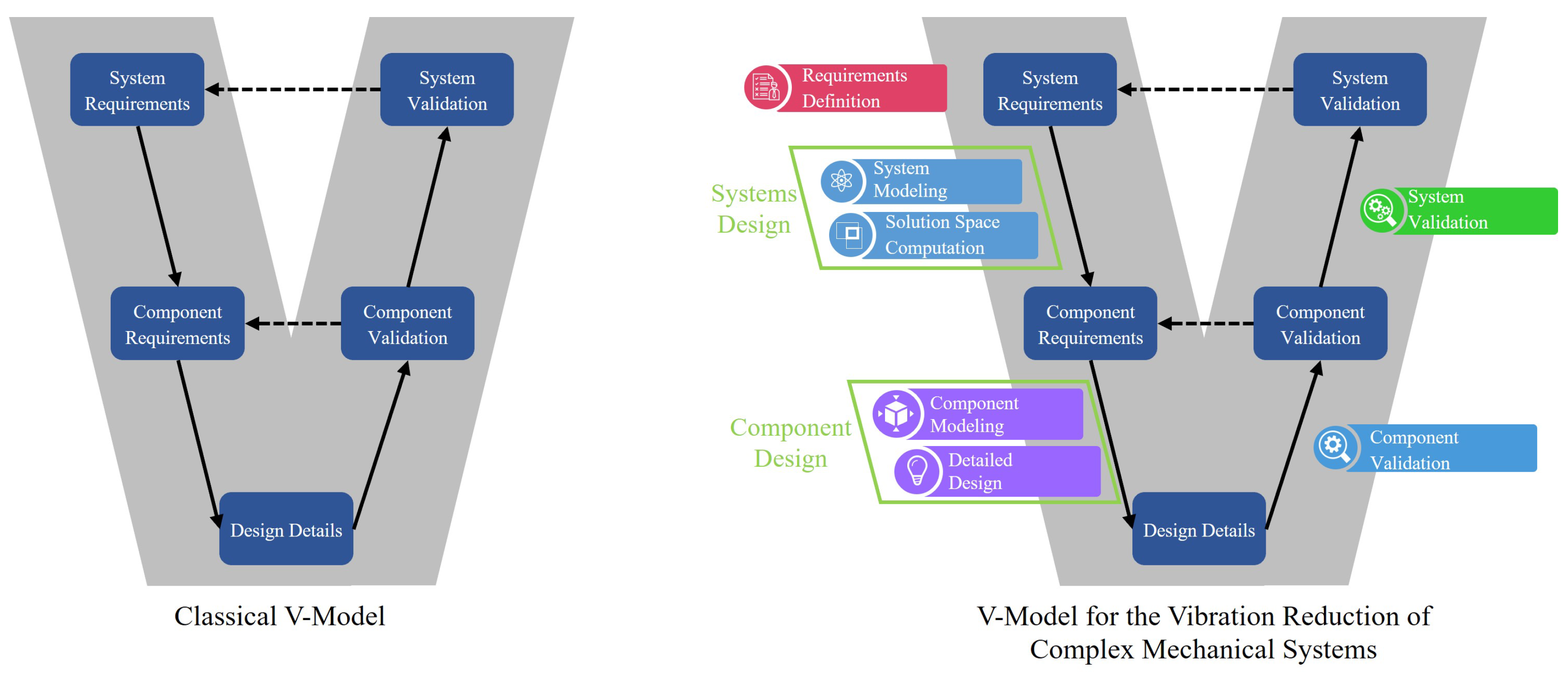
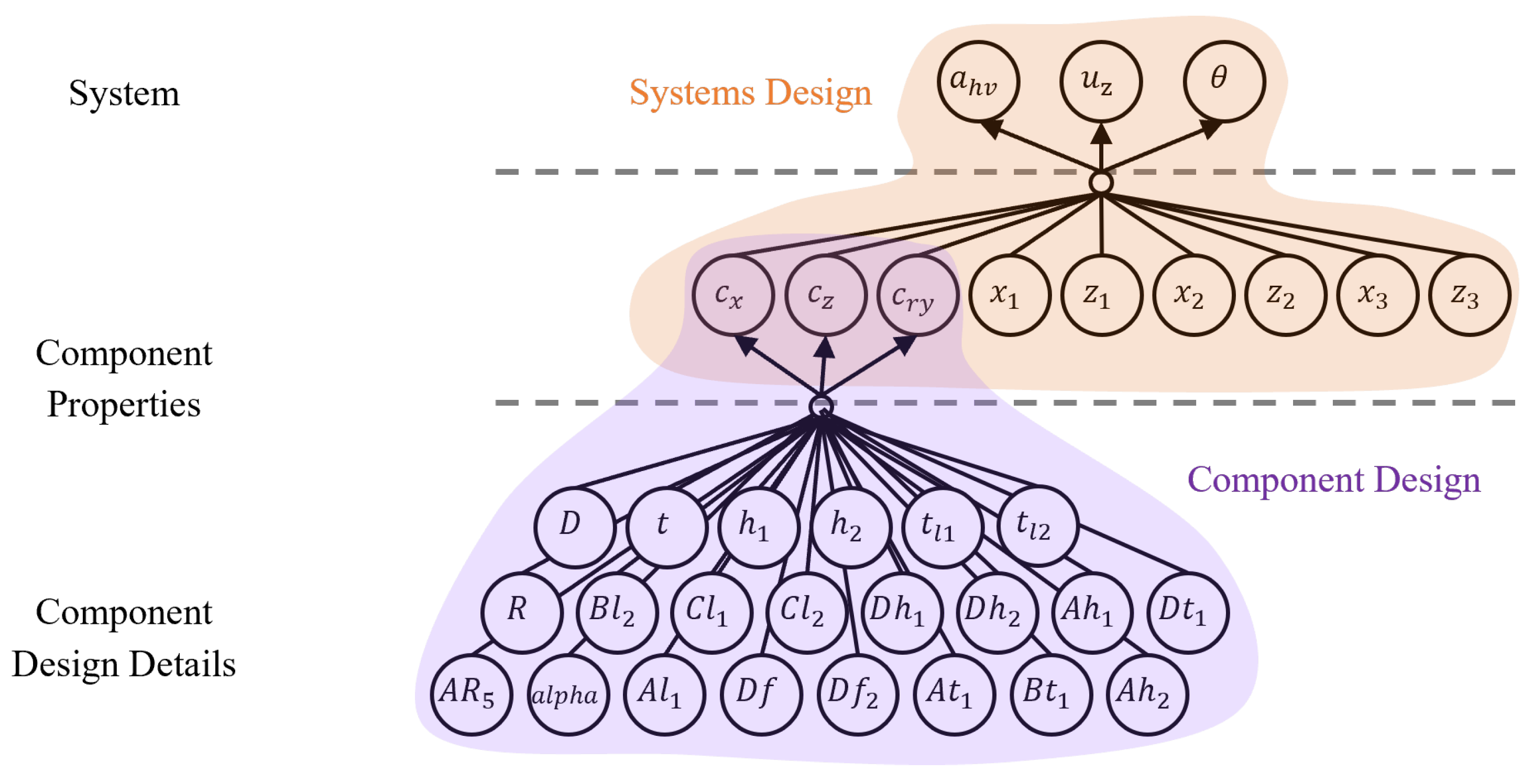
In the beginning of a general product-development process, requirements for the entire system are gathered from customer expectations, from the analysis of competitive products, or from both [
24]. These requirements are defined on quantities that are used to evaluate the system performance (
Figure 1). After the whole system is developed, the performance of the system is validated against the initial requirements. Between requirement gathering and validation is the solution-finding process. The method proposed in this work follows the general idea of system decomposition in the V-model, and the solution-finding process is divided into systems design and component design stages. The proposed method can also cope with decomposition of the structure into further structural hierarchies when this is desired for more complex problems. The system’s design phase consists of two steps: system modeling and solution space computation. The component design can be divided into component modeling and detailed design.
System modeling
Through system modeling, the relationship between the quantities representing component properties (design variables of the systems design problem) and the quantities evaluating the system performance (quantities of interest of the systems design problem) are modeled mathematically. With this model, one can evaluate the system performance based on component properties. This model can be built with various methods depending on the complexity of the problem as well as the desired accuracy and affordable computational cost, for example, with the analytical model [
25], multibody simulation (MBS) [
26], frequency-based substructuring (FBS) [
13], etc.
Solution space computation
Based on the system model and the system requirements, the admissible ranges of component properties that make the system performance fulfilled are identified. This can be done by analytical derivation for simple system models [
25]. For complex system models, numerical methods are needed. One type of method is sampling based [
22,
27,
28,
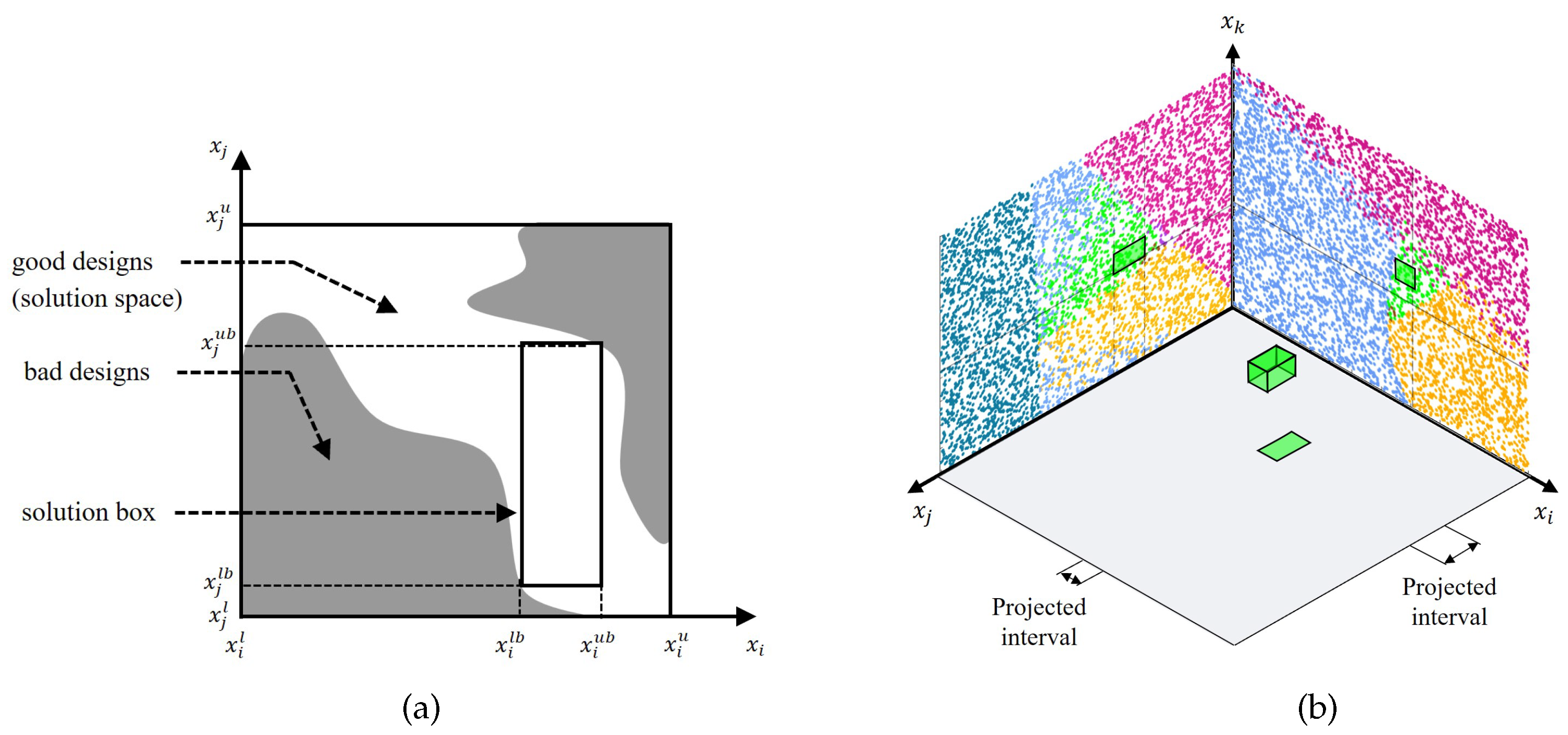
29]. Candidate designs are randomly sampled in the design space and are restricted by the upper and lower limits of each design variable (marked as
and
, respectively, for the design variable
in
Figure 2a). For each sample design, the values of system performance are computed based on the system model for each sample design. These values are then compared to the system requirements. The sample designs that fulfill all system requirements are denoted as good designs, otherwise as bad designs. A set of all good designs represents an admissible area of the values of the design variables and is thus called the solution space [
22] (
Figure 2a). Solution spaces can be visualized by plotting good designs and bad designs together in 2D plots, where two arbitrary design variables are plotted against each other.
In order to decouple the development task for each component, an admissible value range bounded by upper and lower limit values (marked as
and
, respectively, for
in
Figure 2a) is sought for each design variable
. The value ranges of all design variables span an n-dimensional space, also called the solution box. One of the methods used to identify the optimal solution box is selective design space projection [
27], which is also the method adopted in this paper. It projects the design box, which is visualized as a high-dimensional slab of the design space, as shown in
Figure 2b, onto 2D plots. In these plots, good designs are marked in green and bad designs in other colors when certain system requirements are violated. Based on these plots, the ’purity’ of the current solution box can be checked through visual evaluation. The upper and lower limit of each design variable is then manually adapted iteratively toward ’purity’ improvement, until the rectangulars on all plots contain only good designs. This way, the admissible range of each design variable is determined. The system requirements are guaranteed to be fulfilled as long as the values of all design variables stay inside their derived value ranges. In other words, the solution box defined by these value ranges is a sufficient (yet unnecessary) condition to fulfill the system requirements. Further methods for the solution space computation and optimization are stochastic iteration [
22] and corner tracking [
28,
29].
In the following component design phase, the components should be designed in such a way that the component properties stay in these computed value ranges. This means that these value ranges serve as component requirements for the component design. This way, the system level requirements are decomposed into component requirements. Unlike optimization, the solution spaces provide admissible value ranges instead of one single optimal value as component requirements. This provides flexibility and robustness for the component design.
Component modeling
The component properties, which are the design variables in the systems design, now become quantities of interest in component design. In order to fulfill the requirements on component properties, appropriate values for the component details are sought, which are now the design variables. A model of the component is first built to evaluate its performance for specific design details on the component details level. This model connects the component property level in the middle and the design details level at the bottom in the system hierarchy in
Figure 1. This model can be built either with analytical modeling methods [
25], CAD modeling [
30], the finite element method (FEM) [
31] or experimental modeling [
32], which means measuring the property of different designs experimentally. This model provides the basis for the final decision on design details.
Detailed design
Based on the component requirements and the component model, one can either find the right value for the design variables with methods such as numerical optimization [
33] or Design of Experiment (DoE) [
34], or find the right values by comparing them with existing designs.
3. Industry Use Case
In this section, the proposed development method is exemplified by a practical application from the construction industry, the vibratory rammer. First, an introduction to the machine is given. Then, the development requirements as well as corresponding load cases are defined mathematically. In the next step, the system dynamic is modeled with MBS, based on which the solution spaces are computed. In order to reach these solution spaces, proper component designs are sought with optimization and DoE. Finally, a virtual validation is conducted to verify the success of the entire design activity.
3.1. Vibratory Rammer
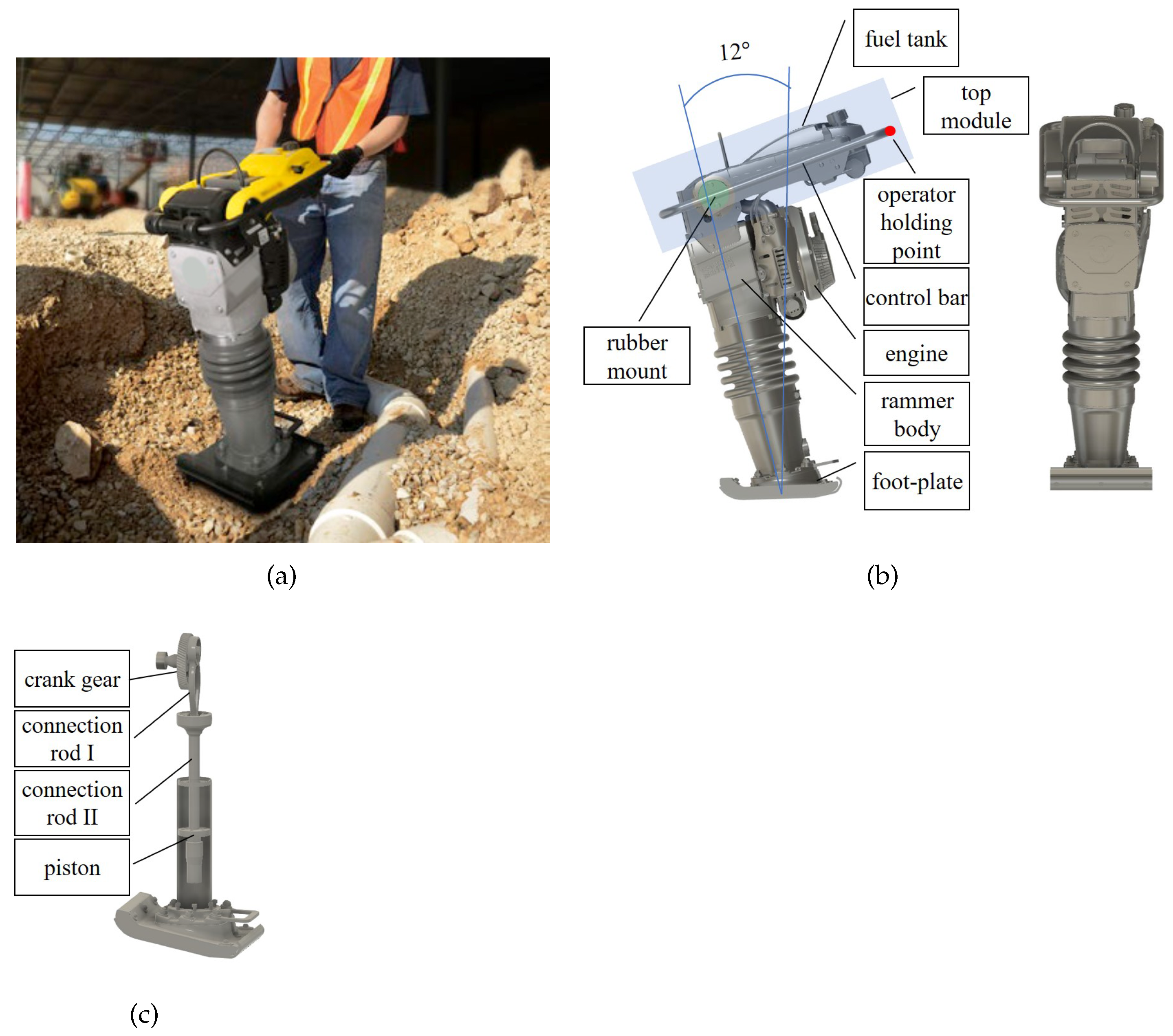
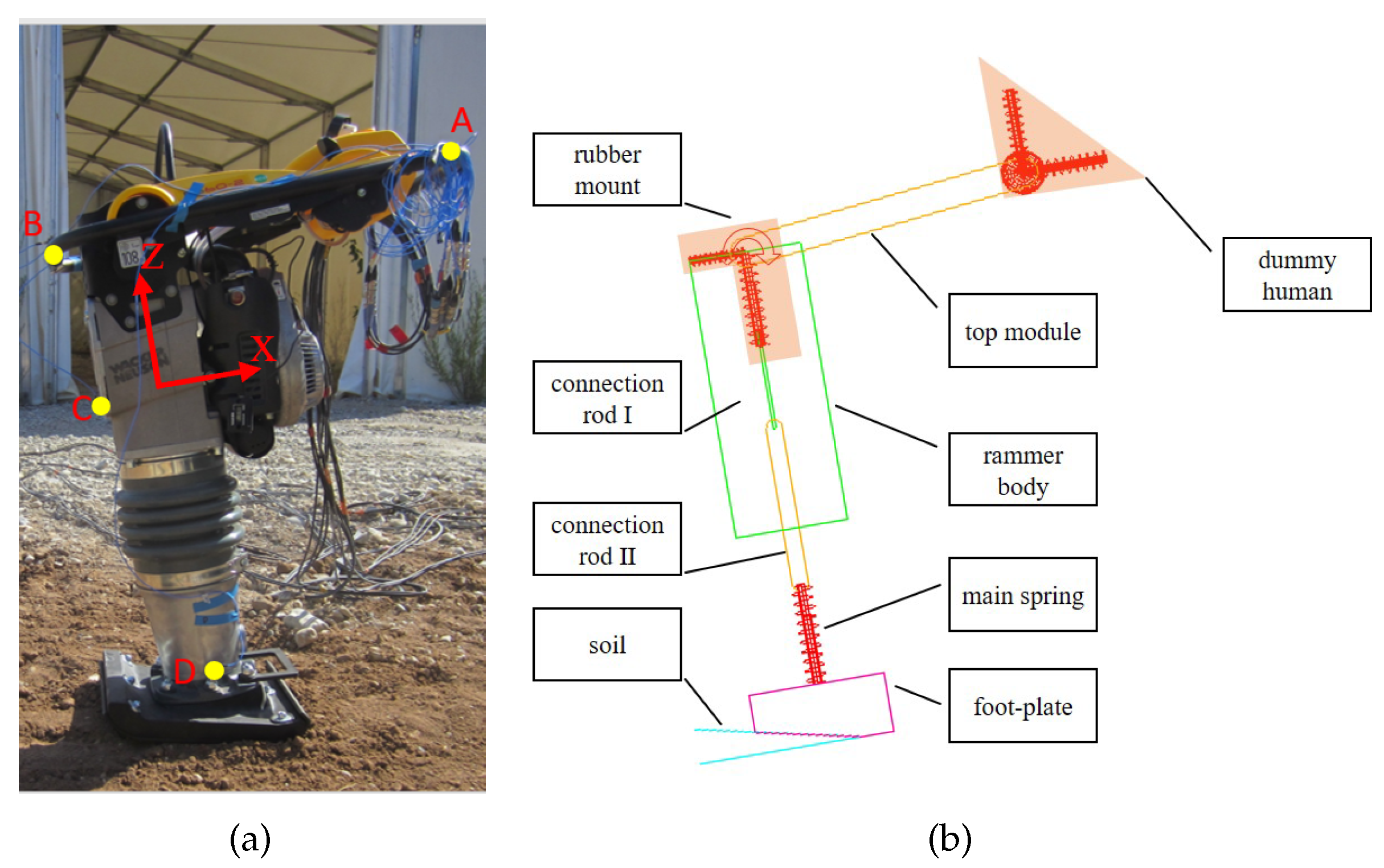
A vibratory rammer is used on construction sites for soil compaction after a certain construction activity is conducted. In the present research, a popular rammer product in the market is taken as an example. The engine and the crank gear are mounted on the rammer body as shown in
Figure 3. The engine drives the rotation of the crank gear, which is connected to a piston through two connection rods. The rotation of the crank gear moves the connection rod II up and down, thus enforcing a periodic relative movement between the rammer body and the piston. This relative movement
can be described as a harmonic function
where
A is the amplitude and
f is the vibration frequency decided by the engine rotation speed. When the piston moves downward, it presses the foot-plate through the rammer main spring. The foot-plate applies a pressure in turn to the ground and compacts the soil. Due to this periodic movement, the rammer ‘jumps’ along the main axis of the rammer body. The main axis has a 12-degree angle to the global vertical axis. Due to this angle, the machine also ‘jumps’ forward besides vertical in operation. In the downward period, the rammer generates an impact on the soil and thus compacts the soil. The top module, which consists of a fuel tank, control bar and accessories, is connected to the rammer body through a vibration isolator (rubber mount). Due to this soft connection, the vibration of the rammer body is transferred less to the holding point of the control bar, where the operator is loaded.
3.2. Design Problem
3.2.1. System Requirements and Quantities of Interest (QoIs)
In the scope of the present research, a vibratory rammer is to be redesigned so that the vibration at the holding point is reduced to a desired level (requirement 1), while the guiding performance must not be worse than in the reference design (requirement 2). By reducing the vibration, the dynamic load on the operators is reduced so that the health of the operator is protected, and the operator can work longer on a daily basis. This will also give the manufacturer of the vibratory rammer an advantage against competitors in the market. During operation, the machine must also follow the operator’s guidance well. This means that when the operator presses the control bar downward, the operator’s hands must be supported with enough stiffness and the machine leans backward so that it can be pushed uphill on a slope. A softer vibration isolator is in general beneficial to the vibration requirement; however, it is unfavorable for good maneuverability. These two requirements are therefore in conflict with each other, which makes it difficult to find effective measures to fulfill both requirements.
The method proposed in
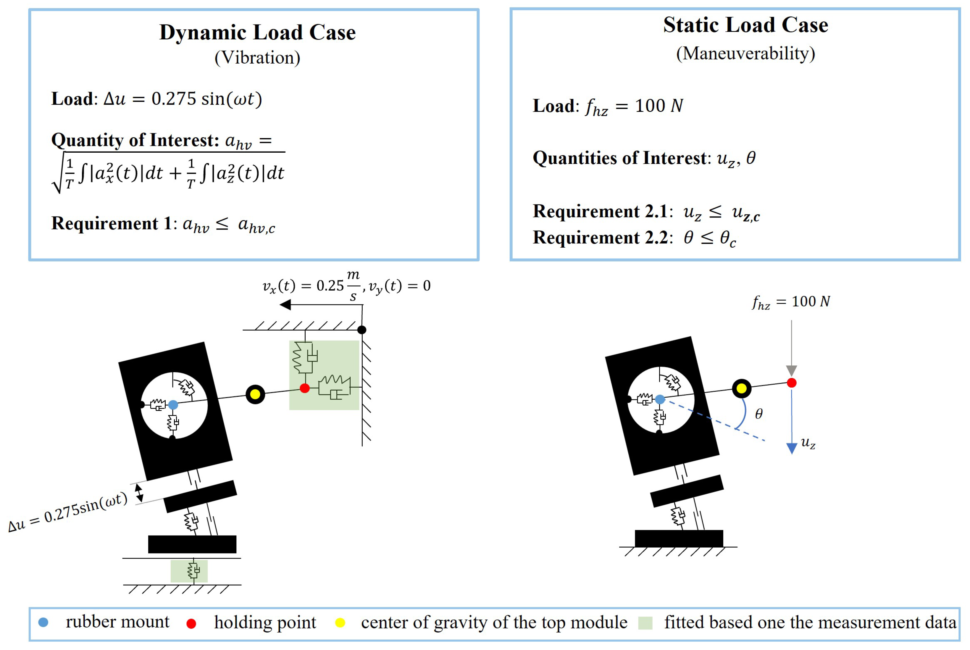
Section 2 offers a systematic framework to find a proper component design for this complex design problem. The first requirement refers to the dynamic performance of the system, while the second requirement involves only its static performance. For better problem solving, the development requirements for the entire system are formulated mathematically in two load cases (
Figure 4). Since the rammer mainly ‘jumps’ upward and forward, the machine dynamics are simplified as a 2D problem.
Requirement 1: dynamic load case
During operation, the rammer mechanism that is driven by the engine enforces a periodic relative movement between the rammer body and the piston with a frequency of 11.55 Hz and an amplitude of 0.275 m (Equation (
1)). This dynamic motion also causes the vibration of the entire machine. In the dynamic load case, the vibration is evaluated by the so-called Hand–Arm–Vibration (HAV) value
[
35] at the holding point of the control bar, which is a commonly used index as an industry standard for vibration regulation to evaluate the dynamic load on humans. It is defined as
where
,
and
are frequency-weighted accelerations in different directions.
T is the total duration of vibration data that is used for the computation of the HAV value. With the HAV value
, the contributions of the dynamic loads in all spatial directions are summed up. In the current case study, however, the dynamic motion is simplified into a 2D problem. Therefore, the HAV value
in this work is calculated as
In the present research, it is desired to reduce the vibration from 14.49 m/s
of the reference design to below 8 m/s
, which is believed to be a reasonable vibration reduction target based on discussions with a rammer manufacturer. Requirement 1 is defined mathematically as
Requirement 2: static load case
Maneuverability also plays a role during operation while the machine is vibrating. However, the maneuverability is barely affected by the vibration level of the machine. On the contrary, it is mainly associated with the static property of the rammer. Thus, the maneuverability is evaluated separately in a static load case. In the static load case, the rotation of the gear is fixed. The foot-plate is fixed to the boundary. The rotation angle of the control bar
and the vertical displacement of the handling point
to a given operation force in the vertical direction
must be smaller than the limit values
and
. It is desired that the maneuverability of the new rammer design is not worse than the reference design. The limit values
and
are therefore defined as the same as those measured
and
values of the reference design.
of the reference design is calculated based on the measured acceleration with Equation (
3). The measurement is shown in
Section 3.3. All system requirements are summarized in
Table 1.
3.2.2. Design Variables (DVs)
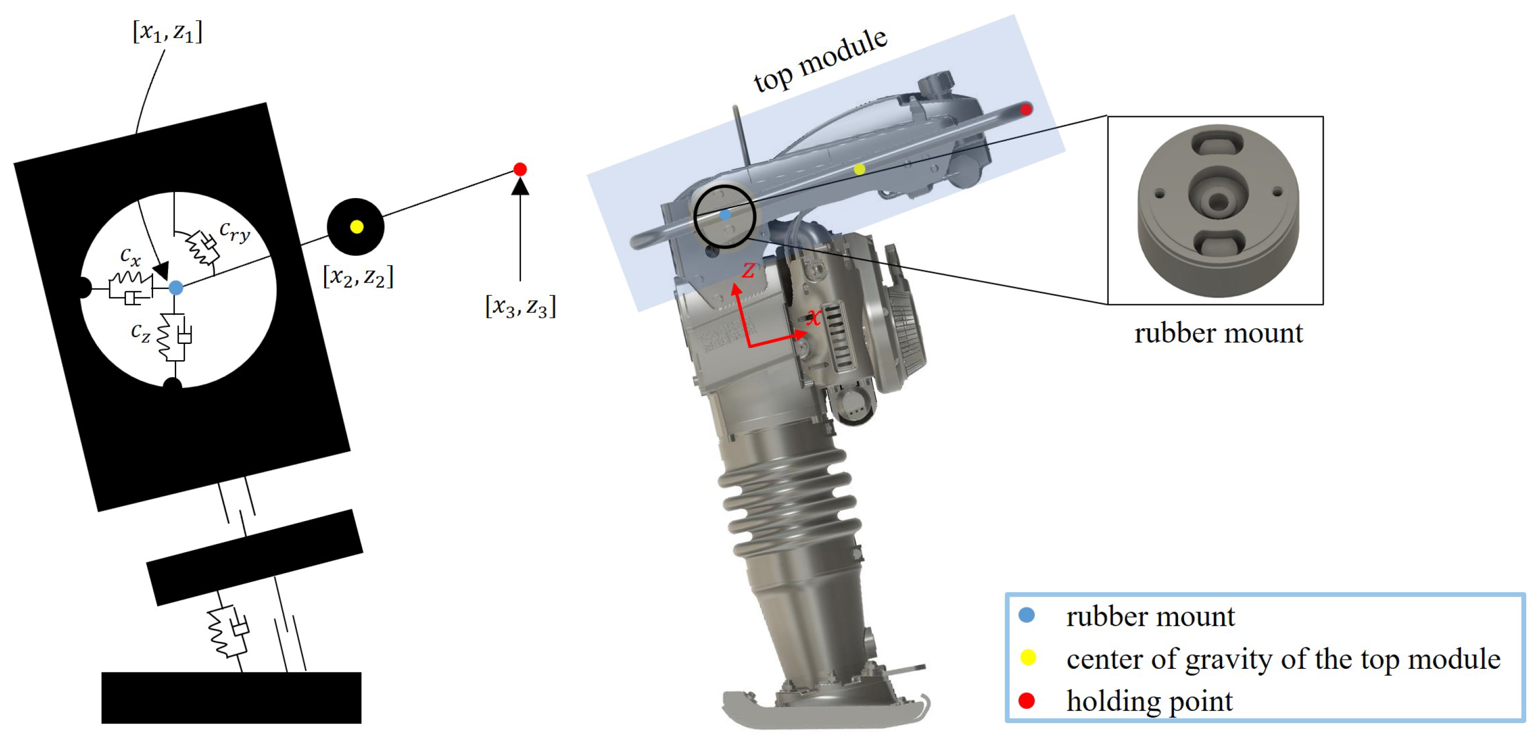
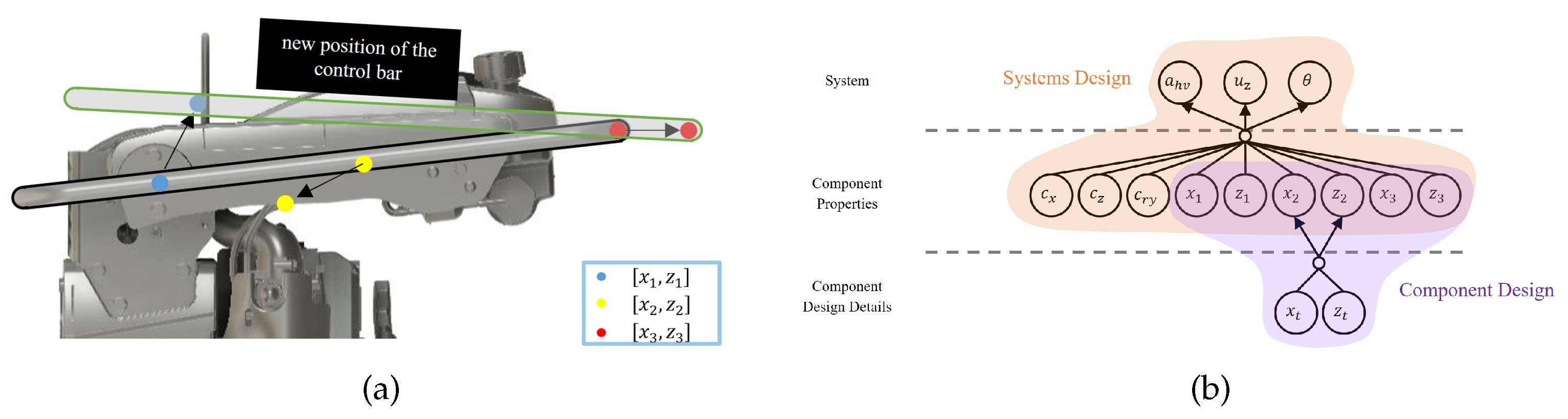
The rubber mount and the top module are to be redesigned so that these requirements are fulfilled (
Figure 5). The mechanical property of the rubber mount is characterized by its stiffness in the horizontal direction (
), vertical direction (
) and rotational direction (
) in the rammer local coordinate system, which further depend on the detailed geometry and material parameters of the rubber mount.
The layout of the top module may also be changed. The geometrical layout of the top module is represented by the position of two key points: the position of the rubber mount (
and
) in the front and the holding point (
and
) in the back. Furthermore, the position of the center of gravity (CoG) (
and
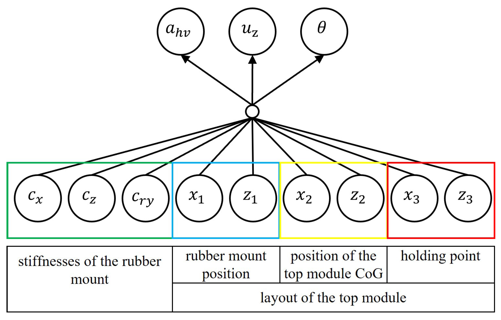
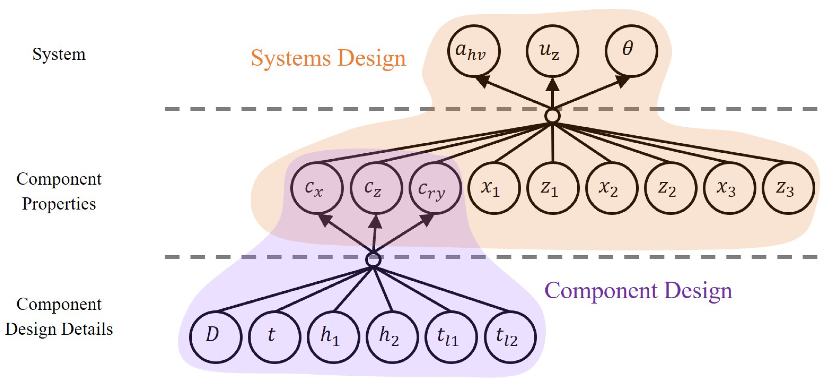
) of the top module also influences the overall dynamics of the machine. The position of the CoG can be influenced, e.g., by moving the position of the fuel tank and thus is also used as a design variable. The design variables and quantities of interest of the systems design are summarized in
Figure 6.
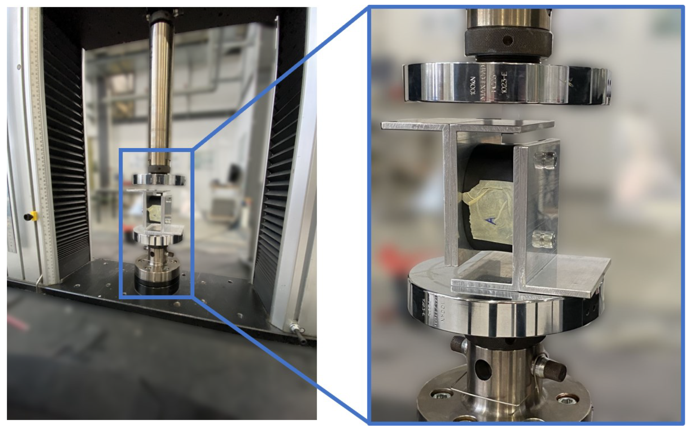
The current values of all design variables are measured for the reference design of the rammer (see the measurement of rubber mount stiffness in
Figure 7, for example) and are summarized in
Table 2. In the design process, these values cannot be changed arbitrarily due to practical limitations such as geometric limitations imposed by other components, cost consideration, user habits/expectations, safety regulations, etc. Reasonable upper and lower limit values for each design variable are defined in cooperation with a rammer manufacturer. These limits define the design space of this design problem.
3.3. Systems Design
3.3.1. System Modeling
MBS model
As discussed in
Section 2, the first step of problem solving is system modeling. Several methods are available for system modeling. The main excitation frequency of the ramming process
f is 11.55 Hz. The contact between the rammer and the soil must be modeled properly. Here, this low-frequency nonlinear dynamic problem is modeled with the Multibody Simulation (MBS) method in MSC Adams
® [
36]; see
Figure 8b. The main parts of the rammer are modeled as rigid bodies: top module, rammer body, crank gear, connection rod I and II, and foot-plate. Their property values, dimension and position in the model are the same as the measured values of the reference design (
Table 3). These rigid bodies are connected by connectors and force elements. The rubber mount is modeled as three springs representing the elastic connection in translational
x- and
z-directions as well as the rotational direction
. In the reference design, there are two rubber mounts of the same design on each side. As a result, the spring stiffness values in the MBS model are twice the stiffness values of each rubber mount.
The dynamics of the soil is modeled with a damper. The contact between the rammer and the soil is modeled with the penalty method. In operation, the rammer is guided by an operator. In the MBS, the dynamics of the operator is modeled as a dummy human consisting of two springs and two dampers. Parameter values of the soil model and the dummy human are not measured directly but are fitted based on the measurement results in
Figure 9. Parameter values of all force elements are summarized in
Table 4.
In order to evaluate the system performance regarding the two system level requirements as defined in
Section 3.2.1, two analyses are conducted. In the dynamic load case, the crank gear is defined to rotate with a constant frequency of 11.55 Hz, the same as the reference design. Due to this rotation, the model ‘jumps’ up and down as well as forward in the dynamic simulation. The acceleration at the holding point is computed for the
x- and
z-direction in the rammer local coordinate system (
and
). For the static load case, the gear is fixed to the rammer body. The foot-plate is also constrained with a fixed boundary condition. A static force
of 100 N in the global vertical direction is defined on the holding point as the external load as defined in
Figure 4. The rotation angle of the control bar
and the vertical displacement
are computed in a static analysis.
The vibration of the rammer in operation is measured at measurement points marked in Figure (
Figure 8a). The data from points A, C and D are used to validate the simulation. The comparison between the acceleration in the time domain shows good agreement between the simulation and the measurement, as can be seen in
Figure 9. Furthermore, the HAV-value
is calculated based on Equation (
3) for both measurement and simulation.
of the measurement is 14.49 m/s
. The simulation has an
value of 14.31 m/s
. The MBS model is considered to be sufficiently accurate.
Surrogate model
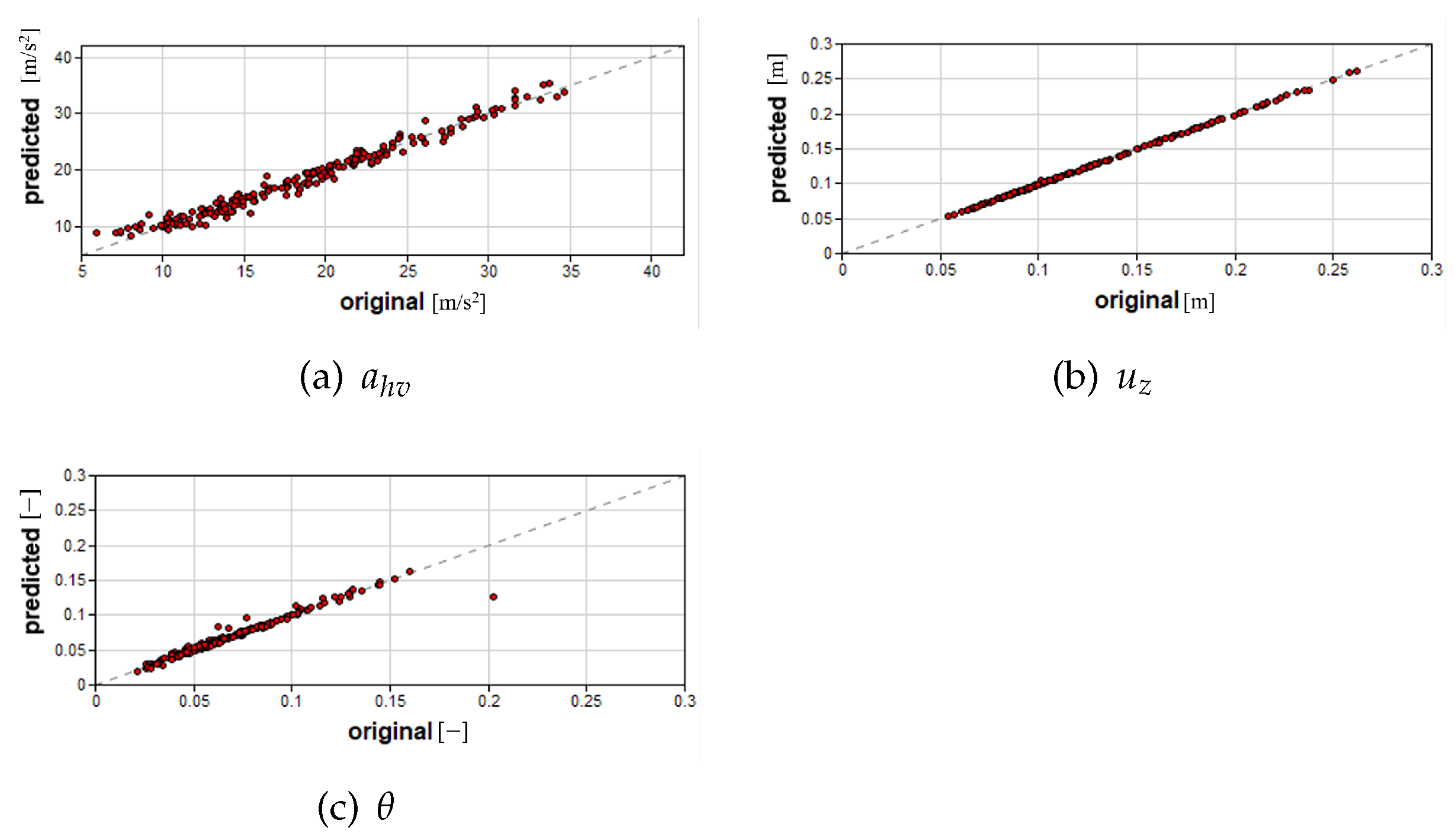
Each dynamic MBS simulation takes about 8 min. The solution space computation in the next section requires thousands of evaluations of the system performance for different sample designs. In order to reduce the computational burden of the solution space computation, a surrogate model is built based on neural network technology. In total, 1000 different designs are generated based on random sampling. The system performance is evaluated through MBS for each set of sample values. These values of design variables (DVs) and quantities of interest (QoIs) are then used to train a neural network model as a surrogate model. The training quality is good, as can be seen in
Figure 10 and
Table 5.
3.3.2. Solution Space Computation
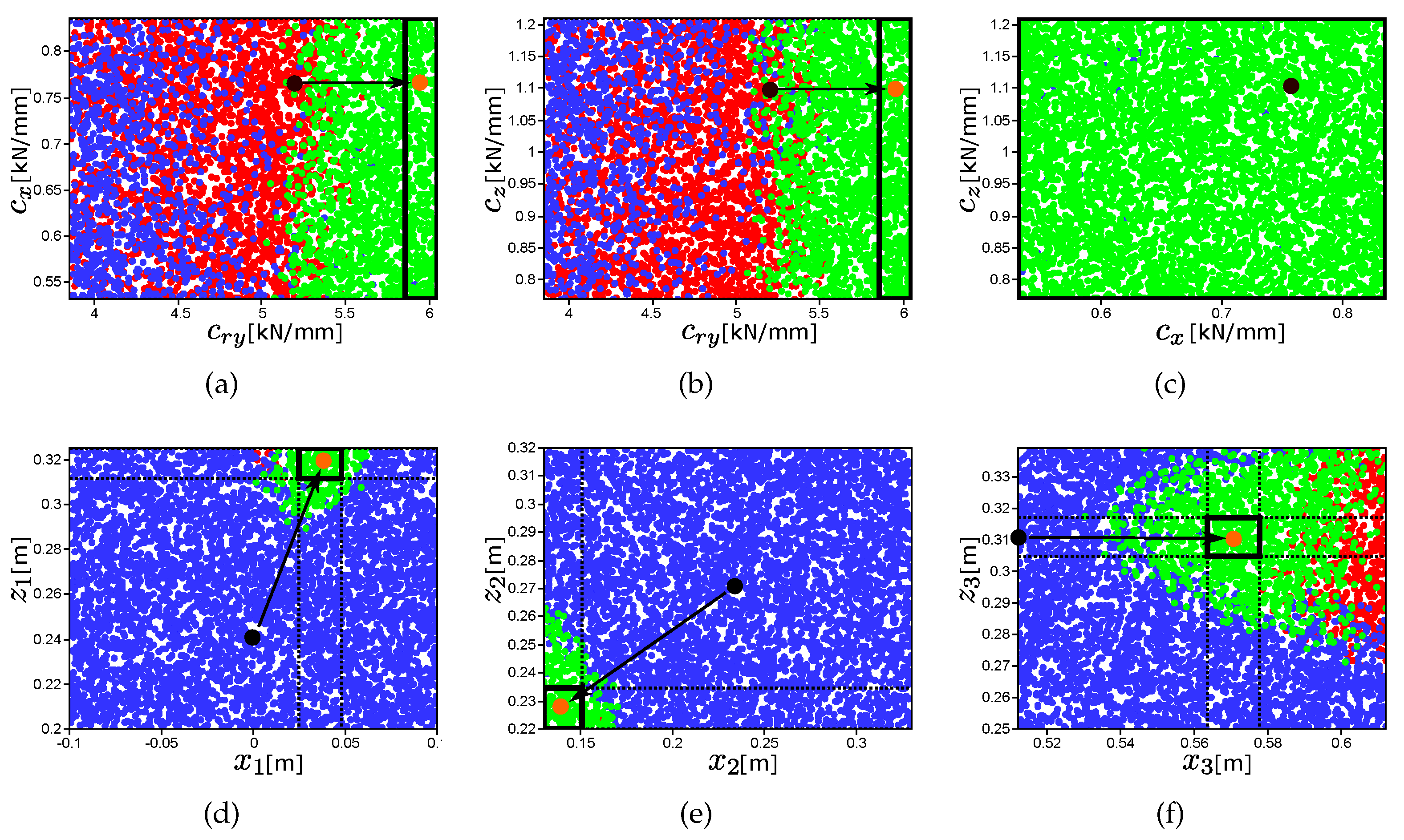
Due to the complex relationship between DVs and QoIs, the component requirements cannot be computed analytically. Instead, the component requirements are computed numerically. The solution spaces are computed with the selective design space projection [
27], and the results are plotted in
Figure 11. Sample designs are generated randomly in the design space. A sample design that violates the dynamic and static requirements is marked in red and blue, respectively. The designs that can fulfill all requirements are marked in green. Rectangular solution boxes are created in order to decouple the requirements on design variables. Based on the solution boxes, the admissible value range for each DV is identified, which serves as the component requirement in the following component design (
Table 6).
The reference design is marked with black points in the design space based on the values in
Table 2. As can be seen in
Figure 11, the reference design is outside of the solution space and does not fulfill the component requirement. By comparing the position of the reference design and the solution box in the design space, it is concluded that the following changes must be made for the rubber mount and the top module in order to fulfill the system requirements in
Table 1:
Rubber mount
Top module
must be increased. This means that the rubber mount must be moved to a higher position.
and must be decreased. The center of gravity must be moved forward and downward. This can be achieved by repositioning the fuel tank.
A larger value of is desired. The holding position must be moved away from the engine (in positive local x-direction).
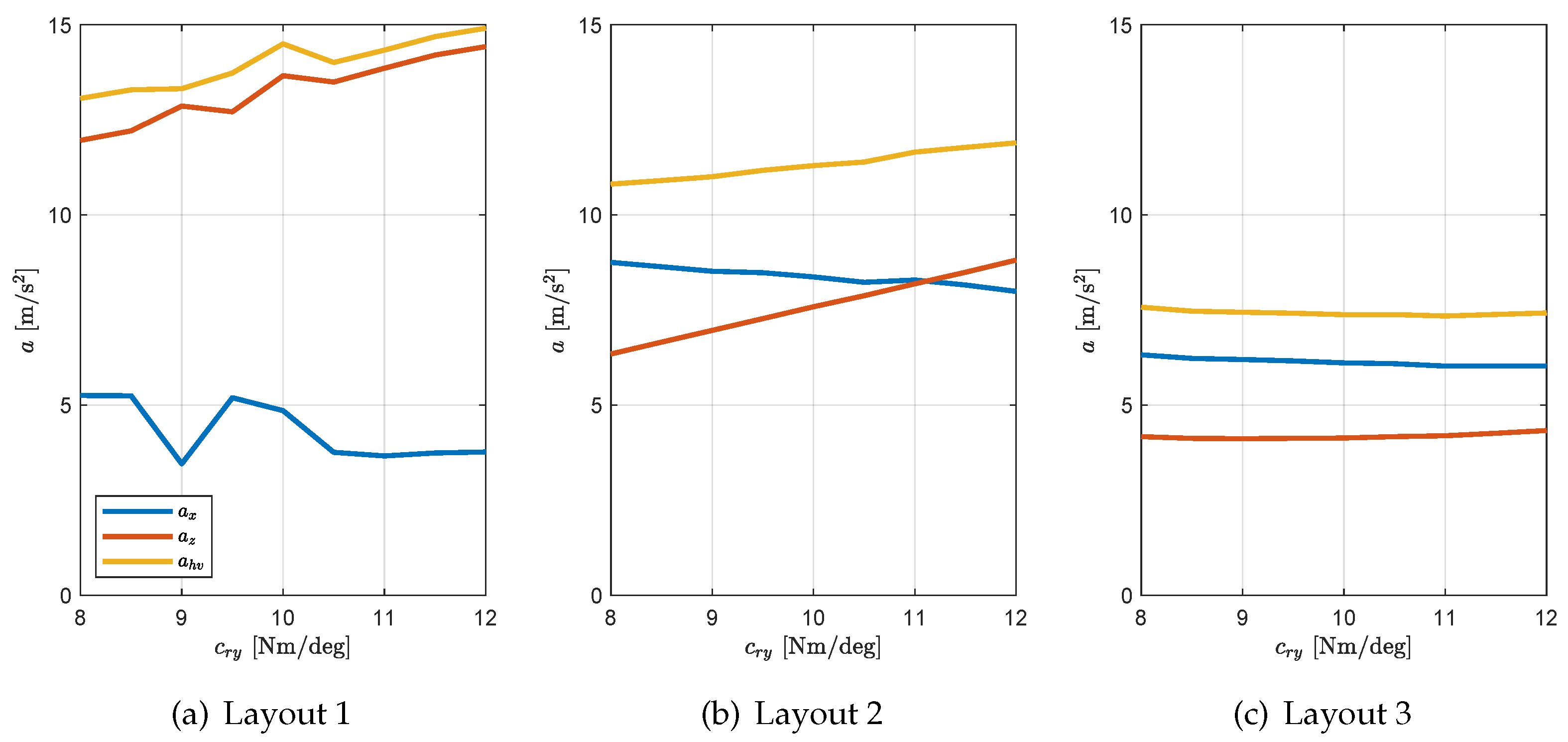
Interaction between top module layout and rubber mount stiffness
It was found that in order to reach a lower vibration level as demanded by the system level requirement R1, the rotational stiffness should be increased. This is somehow counter-intuitive, since a softer vibration isolator is in general beneficial for vibration reduction. This is presumably because the change of the top module layout (
,
,
,
,
and
) influences the dependency of the vibration level on the rotational stiffness of the rubber mount. In order to verify this hypothesis, a sensitivity study was conducted for three different layouts (
Table 7). Layout 1 is the one of the reference design. Layout 3 is an example design inside the solution space. Layout 2 is an intermediate layout, where
,
,
and
are the same as in layout 1, but
and
are changed to be the same as in layout 3.
As can be seen in
Figure 12, a higher rotational stiffness of the rubber mount increases the vibration level in the vertical direction (
z-direction) in all three layouts but decreases the vibration in the horizontal direction (
x-direction). Since the overall vibration level depends on the contribution of vibrations in both directions, whether the overall vibration level increases or decreases depends on the relative value of the vertical and horizontal vibrations. In layout 1, the vertical vibration is much larger than the horizontal vibration, thus dominating the change in the overall vibration. An increase in the rotational stiffness increases the vertical vibration and thus the overall vibration. Layout 2, however, lowers the vertical vibration in general compared to layout 1. This makes the vertical and horizontal vibration approximately the same level. The overall vibration is more influenced by the vertical vibration when the rubber mount is stiff; however, it is dominated more by the horizontal vibration when the rubber mount is soft. In layout 3, the vertical vibration is even smaller. An increase in the rubber mount stiffness slightly decreases the overall vibration level.
This explains why a lower vibration level is associated with a stiffer rubber mount in the final solution space. This also shows the complex interaction between different design variables. The influence of a certain design variable on system performance depends on the specific value of other design variables. Due to this interaction, there is no obvious tendential dependency between a certain quantity of interest and a certain design variable. Thus, this complex design problem cannot be solved by a linearized sensitivity analysis based on the reference design. Instead, solution spaces guide a way toward a solution taking component interaction into account.
3.4. Component Design
3.4.1. Component Modeling
Rubber mount
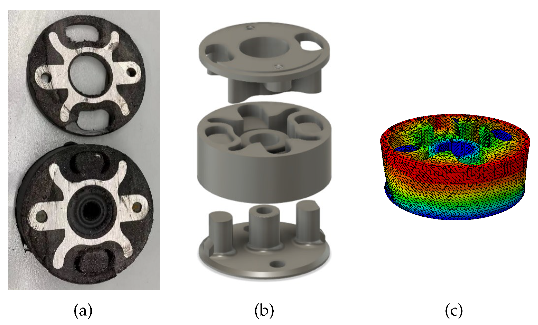
The rubber mount consists of two metal connection parts and the rubber in between. Their dimensions are measured in the reference design. Several rubber mount samples are cut in different directions to check the inner geometrical details (
Figure 13a, left), based on which the concrete geometry of the rubber part is modeled in a CAD model (
Figure 13b). The rubber part is then modeled with FEM in Abaqus
® (
Figure 13c) [
37]. In order to determine the rubber mount stiffness
,
and
in the simulation, three load cases are defined. In each of them, one side of the rubber is constrained, while the other side is loaded either in the
x-,
z- or
-directions with a unit force or moment. The stiffness is calculated as the load divided by the resulting displacement or rotational angle. The rubber is modeled as an isotropic material. Proper parameter values are sought through model updating by comparing the simulated stiffness in the
x-,
z- and
-directions to the measured stiffness in
Table 2. Finally, the Young’s modulus of 2.06 MPa and position’s ratio of 0.422 are identified. The absolute deviation between the simulated and measured stiffness is below 4% (
Table 8). The FE model is considered as valid.
Top module
The layout of the top module must also be changed in order to fulfill its requirements. The design variables are marked in
Figure 14a and are highlighted in
Figure 14b. All values of these quantities between the lower and upper limits in
Table 6 can fulfill the requirements. In the present research, the values of the example design in solution spaces in
Table 7 are adopted as final values. If the position of the rubber mount
and the holding point
are moved accordingly, the new control bar should be moved to the position marked in green in
Figure 14a.
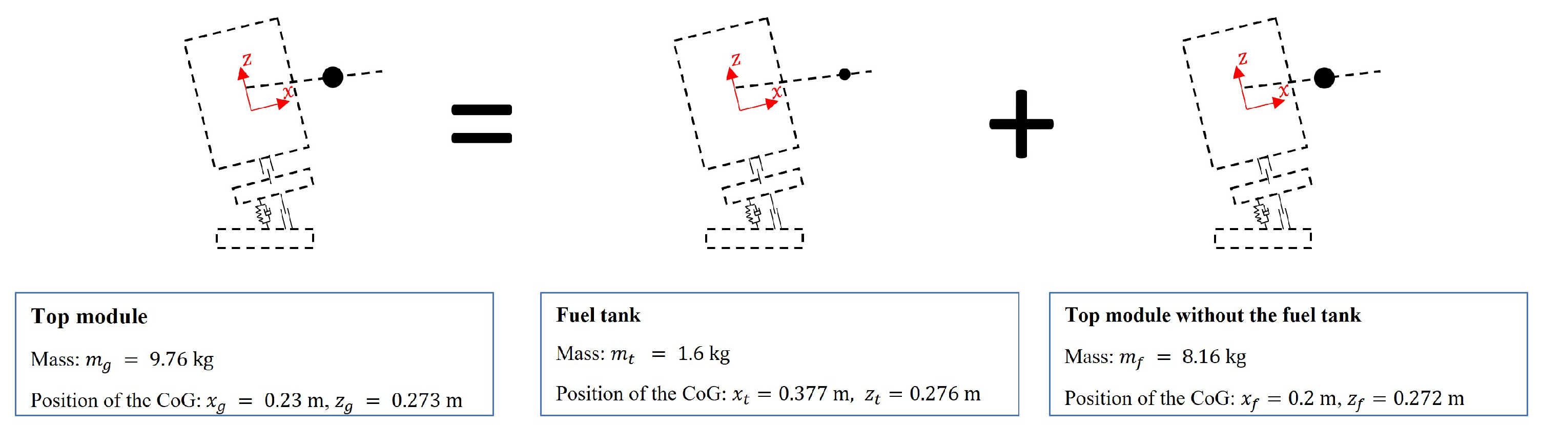
In order to move the center of gravity to the targeted position, the fuel tank is re-positioned. The exact position is determined by dividing the top module into two parts: the fuel tank and the rest of the top module (
Figure 15). The fuel tank is simplified as a point mass. Its total mass is 1.6 kg when the tank is half-full. Its original position
is
in the local coordinate system. The rest of the top module is still modeled as a rigid body. The mass is 8.16 kg. The position of the center of gravity is located at
. Based on this component model, the new position of the fuel tank is computed in the next section.
3.4.2. Detailed Design
Rubber mount
Based on the rubber mount model, rubber mount designs that can fulfill the component requirements from
Table 6 are sought. Only the geometry of the rubber mount is to be modified since it is difficult to change the material parameter to a specific target value in the manufacturing process. This design process can be supported with two methods: optimization and DoE. In the following, both methods are applied to demonstrate their applications in the scope of the systemic development method proposed in this paper. A comparison of both methods is not intended.
Numerical optimization identifies values of DVs that minimize the value of the objective function. In order to satisfy the component requirements, the objective function is defined such that the rotational stiffness
is ideally as close to the middle between the upper and lower limit as possible:
subject to
With the two constraints on stiffness in the
x- and
z-directions, they are forced to fulfill the component requirement. The DVs in the systems design problem,
,
,
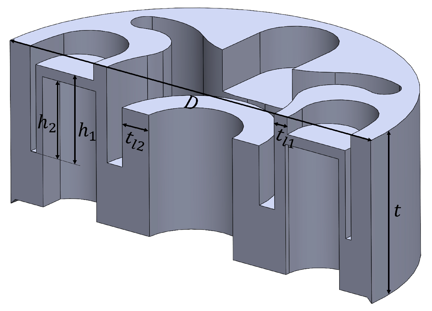
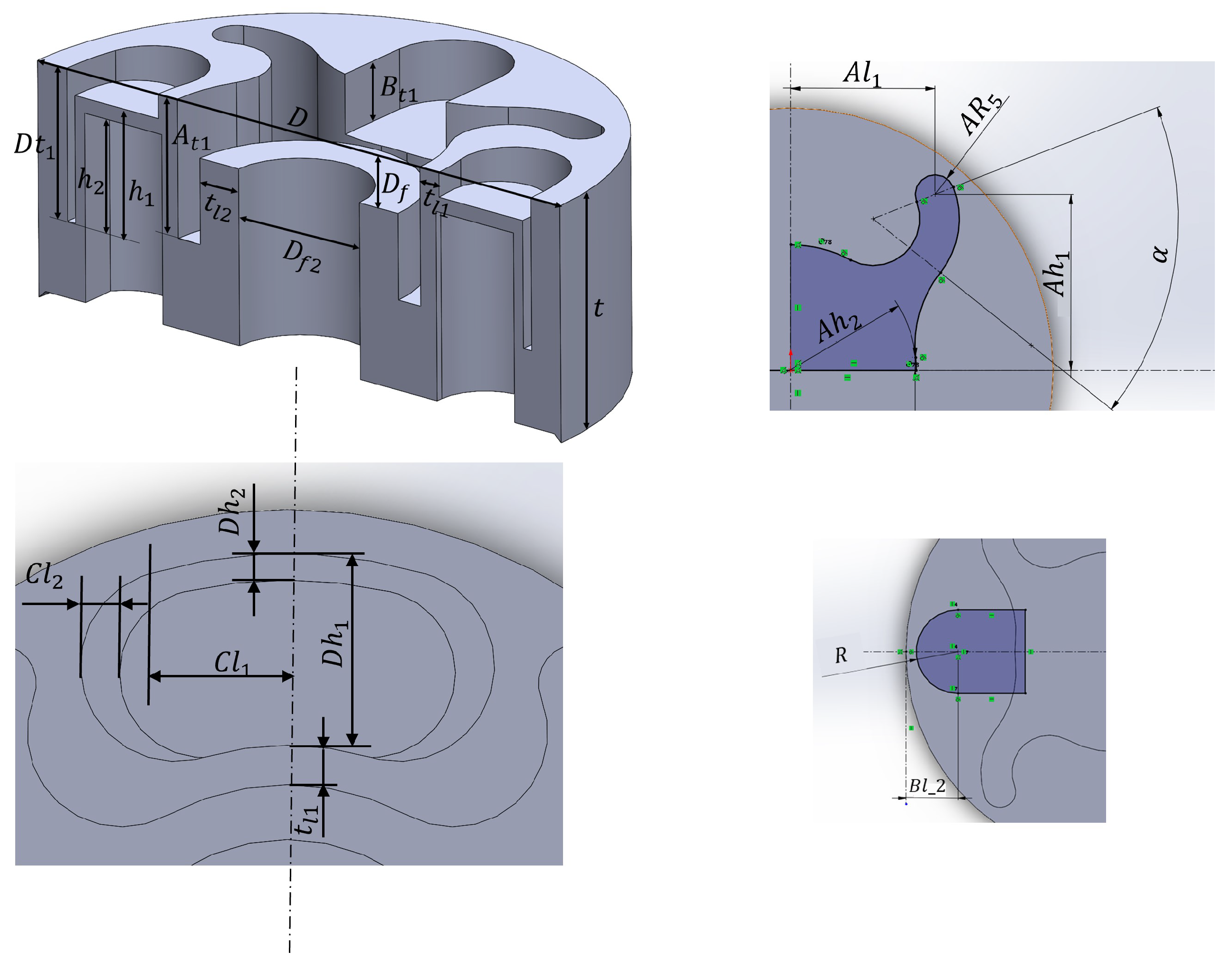
, now become QoIs of the component design problem. In order to fulfill the component requirements on these three quantities, six geometrical parameters are selected as design variables (
Figure 16), including
The global diameter D and thickness t;
Two local heights ( and );
The thickness of two local rubber layers ( and ).
The new DVs and QoIs are summarized in
Figure 17.
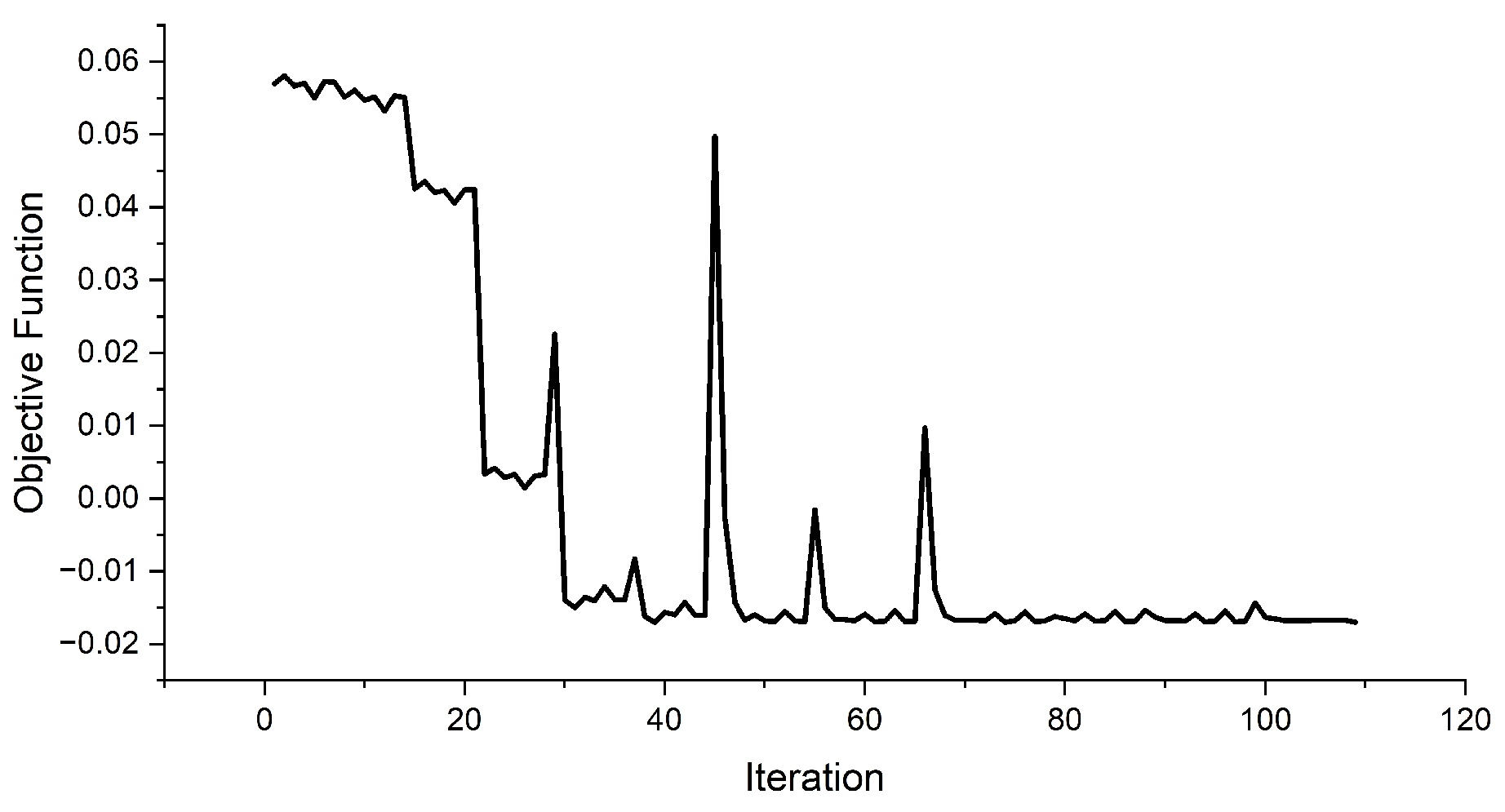
The optimization is implemented in the software Isight
® [
38]. A parametric CAD model is built. The value of the objective function is minimized iteratively with the Sequential Quadratic Programming (SQP) method [
39]. The optimization converges after 117 iterations (
Figure 18). The results are summarized in
Table 9. The targeted value ranges of all three stiffness are reached.
An alternative method used to identify a detailed design is based on DoE. To increase the design space, the rubber mount design is extended with 16 further geometrical parameters (
Figure 19). Finally, 22 geometric design variables are considered (
Figure 20). Optimizing the rubber mount structure with these 22 DVs is CPU-consuming and may not be possible due to the limited 3D modeling capabilities of FE software. Therefore, an automatic workflow combining (1) random sampling-based design of experiments (DoE), (2) parametric CAD modeling, and (3) FE simulation enables automatic and efficient design of the rubber mount.
A new parametric CAD model representing the rubber mount was generated based on the reference model. Design variables are automatically modified in the parametric CAD model by collecting parameter values from the input data and by adapting geometry to maintain consistency. The CAD models representing different designs are automatically generated as preparation for the FE simulation part of DoE. Each CAD model generated from the previous step is then imported into Abaqus for generic and specific simulation setups for the computation (meshing, etc.). Lastly, the simulation result is saved in the results data that cover the stiffness
,
and
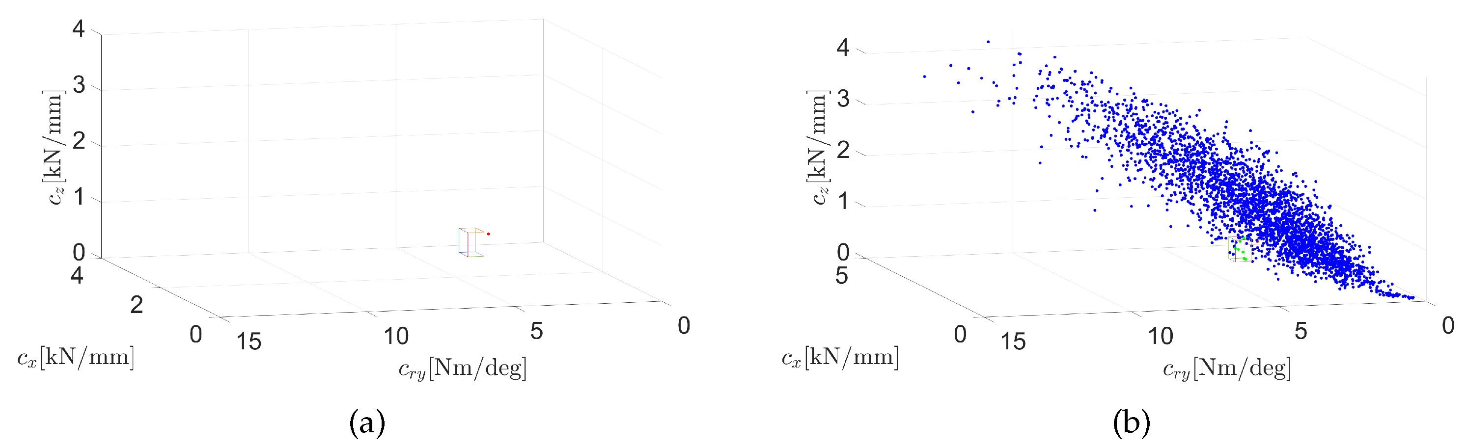
. Admissible areas of the rubber mount stiffness are marked in
Figure 21a based on the component requirements in
Table 6. The red point represents the reference design, which does not fulfill the requirements on stiffness.
In order to find solutions in the solution space of the system level by scanning the entire design space (
Table 10), 3000 samples were randomly created (
Figure 21b). Finally, seven solutions were identified from these random samples that were used to search the 22-dimensional design space; see
Table 11. The identified designs show large differences between each other in terms of internal details and overall size. Even though the geometries are different, they all meet the component requirements on rubber mount stiffness.
Top module
In order to move the CoG of the top module to the targeted position of
, the new position of the fuel tank
is calculated as:
3.5. Results and Validation
The property values of the new rubber mount design and top module design from
Section 3.4.2 are summarized in
Table 12. Here, the rubber mount design through numerical optimization is adopted as final design, although a result from the DoE could have also been chosen. The new design is plotted in the design space and is compared with the solution boxes in
Figure 11. The component requirements are all fulfilled.
In the end, the system performance with the new component designs is validated against the system requirement defined in
Table 1. However, it is time-consuming and cost-intensive to build the prototype for the new design for validation purposes, especially for the rubber mount, where a new mold must be manufactured for the vulcanization process to cope with the new rubber mount geometry. Instead, the system performance is validated virtually with the full MBS model by updating the stiffness values of the rubber mount and the layout values of the top module with the values of the new component designs as listed in
Table 12. As can be seen in
Table 13, the HAV value is reduced from 14.33 m/s
of the reference design to 7.39 m/s
. This is below the limit value of 8 m/s
. A reduction of 48% is achieved. In addition, the maneuverability is also improved slightly. The system requirements are fulfilled.
4. Discussion
The proposed method offers a systematic design framework for the design for vibration reduction of complex vibrating systems. Admissible value ranges of the component properties are identified with a sampling-based design method based on a system model and system requirements. These value ranges serve as component requirements in the component design. Component requirements provide quantitative targets for component design and help component designers identify effective measures faster during component design.
This proposed top–down design process using solution spaces improves the efficiency of the development of complex vibrating machines. The component requirements are computed based on an accurate system model and quantitative computation. These component requirements are consistent with the system requirements. As long as the component requirements are fulfilled, the system requirements are guaranteed to be fulfilled. In this way, design iterations are limited to the component design. Time-consuming design iterations on the system level, which are usually inevitable with existing development methods, are avoided with the proposed method as shown in the presented application example. This reduction of iterations reasonably contributes to efficiency improvement. Furthermore, the proposed method can handle design problems subject to multi-disciplinary system requirements and decompose these requirements into multiple component requirements. The computed component requirements are independent of each other. Each component can be developed by the corresponding department or engineer independently. This enables concurrent engineering. Parallel development of different components further improves the efficiency of the entire development.
This proposed method lowers the complexity and difficulty in the development process. First, the solution spaces improve the robustness and flexibility of the development. Component requirements are formulated as admissible value ranges for each quantity instead of a single target value. This provides tolerance for the uncertainty in the component design and makes it easier for the component designer to reach the design goal. Second, no assumption is made about components when computing the component requirements. For example, all vibration isolator concepts can potentially be applied in the use case of the vibratory rammer. Further concepts other than the rubber mount may also be explored when a certain component concept has difficulties fulfilling the component requirements. This greatly increases the freedom of the solution finding. Furthermore, the development of an entire system is decomposed into two stages through the target cascading process, the systems design and the component design. In each stage, the scope is limited to a certain detail level. This simplifies the development and lowers the difficulty.
Applicability of the proposed method. The proposed method can be extended for a large variety of problems. For problems with different complexity, different system modeling techniques can be adopted. For example, for linear vibration problems, dynamic substructuring can be applied [
23]. For more complex problems, nonlinear dynamics and multidisciplinary requirements should be included in the modeling process. However, care must be taken regarding the modeling effort when choosing the appropriate modeling method. Besides the effort required to build the system model, each analysis with the system model should also not take too long since the solution space computation would require thousands of system performance evaluations. This could be especially challenging for complex systems. Therefore, unnecessary details should be avoided in the model. Model order reduction techniques or surrogate modeling techniques may also be adopted.
Another limitation is that the system topology (e.g., the number of components and the connectivity between components) of the structure to be designed must be known and stay unchanged when applying the proposed method, although changing the system topology may potentially improve the vibroacoustic performance of the whole structure. This is due to the fact that the system modeling is based on a given system topology in general, which is determined in a previous conceptual design phase. With the proposed method, only parameter values are designed. Therefore, the proposed method may encounter difficulties in assisting the development of the next generation of a mechanical product where the system topology undergoes radical changes during the conceptual design phase. However, if the system topology (for example the number of components or the connectivity between components) could also be parameterized in certain application cases, the system topology can also be designed with the proposed method. In these cases, the system topology is no longer a limitation.
5. Conclusions
We present a product development method to design complex vibrating mechanical systems through quantitative requirement derivation with solution spaces. For the first time, it is applied to a full-scale industry problem to demonstrate applicability and effectiveness. The development of a complex vibrating system is decomposed into two steps: systems design and component design. In systems design, the relationship between the system performance and the component properties is modeled quantitatively. Based on this system model, admissible areas of the component properties are derived and expressed as solution spaces. These admissible areas are used as component requirements that are to be fulfilled by the following component design.
The proposed method is demonstrated with an industry use case, a vibratory rammer. As system requirements, the vibration should be reduced while the maneuverability should not deteriorate. These should be accomplished by modifying the rubber mount and the layout of the top module. In this sense, this is a multi-disciplinary multi-component design problem. The nonlinear dynamics of the rammer in operation are modeled with multibody simulation. To reduce vibration, a lower rubber mount stiffness would be beneficial. However, this would lead to worse maneuverability. This conflict of goals is solved by introducing further design variables, the geometric parameters of the layout of the top module. As the number of the design variables increases, this design problem becomes so complex that numerical methods are important for supporting the design process. Based on the MBS model as the system model, the admissible value ranges of the rubber mount stiffness and the position of three geometrical key points determining the layout of the top module are computed as solution spaces. This way, the system requirements regarding vibration reduction and maneuverability are cascaded down to the component level for the rubber mount and the layout of the top module. In order to fulfill these component requirements, the rubber mount and the layout of the top module are modified in the component design. In the end, the system performance is validated virtually, and all system requirements are fulfilled. The effectiveness of the proposed method is validated through the application on the vibratory rammer.
By decoupling different variables in the solution space computation, a certain number of good solutions are excluded from the solution box. This loss of solution space will be quantified in future research, and its influence will be studied. Furthermore, the solution boxes are defined manually using selective design space projection by the author based on the originally computed solution space. In the future, possible techniques to automatically identify optimal solution boxes and to maximize the size of solution boxes shall be adopted. The effectiveness of the proposed method needs to be verified by more applications. Finally, the efficiency improvement needs to be quantitatively studied by comparing the development time using the proposed method to the time using other development methods when applying them to the same design problem.
Author Contributions
D.X.: Conceptualization, Methodology, Software, Writing—original draft, Writing—review and editing, Visualization; Y.Z.: Methodology of DoE, Software, Writing—original draft, Visualization; M.Z.: Supervision, Writing—review and editing. All authors have read and agreed to the published version of the manuscript.
Funding
This research was funded by Zeidler–Forschungs–Stiftung, grant number ZFS-207.
Acknowledgments
The help of Fernando van der Vinne, Joy Dutta, Yuxin Wang and Gabriel Albalá Cervantes from the Technical University of Munich with the simulation and measurement is greatly acknowledged.
Conflicts of Interest
The authors declare no conflict of interest. The funders had no role in the design of the study; in the collection, analyses, or interpretation of data; in the writing of the manuscript; or in the decision to publish the results.
References
- Sacka, M.L. A System Engineering Approach to Improving Vehicle NVH Attribute Management. Ph.D. Thesis, Massachusetts Institute of Technology, Cambridge, MA, USA, 2008. [Google Scholar]
- Hesse, C.; Biedermann, J. Vibroacoustic Evaluation and Optimization of Aircraft Cabin Concepts-A Systems Engineering Framework. In Proceedings of the INTER-NOISE and NOISE-CON Congress and Conference Proceedings, Madrid, Spain, 30 September 2019; Volume 259, pp. 5510–5521. [Google Scholar]
- Haskins, C. Systems Engineering Handbook; Incose: San Diego, CA, USA, 2006. [Google Scholar]
- Angrick, C. Subsystemmethodik für die Auslegung des Niederfrequenten Schwingungskomforts von PKW; Cuvillier Verlag: Goettingen, Germany, 2017; Volume 5. [Google Scholar]
- Ambardekar, M.; Solanki, N. Performance cascading from vehicle-level NVH to component or sub-system level design. SAE Int. J. Veh. Dyn. Stability NVH 2017, 1, 58–65. [Google Scholar] [CrossRef]
- Zeng, P.W. Target setting procedures for vehicle powerplant noise reduction. Sound Vib. 2003, 37, 20–23. [Google Scholar]
- van der Linden, P.J.; Wyckaert, K.; van der Auweraer, H. Modular vehicle noise and vibration development. In Proceedings of the Inter-Noise 2001-Abstracts From International Congress And Exhibition On Noise Control Engineering, Hague, The Netherlands, 27–30 August 2001. [Google Scholar] [CrossRef]
- Mori, T.; Takaoka, A.; Maunder, M. Achieving a vehicle level sound quality target by a cascade to system level noise and vibration targets. In Proceedings of the SAE 2005 Noise and Vibration Conference and Exhibition, Traverse City, MI, USA, 16–19 May 2005. [Google Scholar] [CrossRef]
- Fischer, J.C.H. Methoden für die Validierung des Fahrzeuginnengeräusches von Elektrofahrzeugen in Bezug auf tonale Geräusche Aufgrund Torsionaler Anregung durch den Elektromotor= Methods for the Validation of Electric Vehicle Interior Noise with Regard to Tonal Noise due to Torsional Excitation by the Electric Drive; Karlsruhe Institute of Technology: Karlsruhe, Germany, 2018. [Google Scholar] [CrossRef]
- Muenster, M.; Lehner, M.; Rixen, D. Requirement derivation of vehicle steering using mechanical four-poles in the presence of nonlinearities. Mech. Syst. Signal Process. 2021, 155, 107484. [Google Scholar] [CrossRef]
- Bergen, B.; Chavan, J.A.; van de Rostyne, K. Target setting for vibration transmission through driveline components based on on-vehicle and on-bench evaluation. In Proceedings of the Automotive Acoustics Conference 2019; Springer: Berlin/Heidelberg, Germany, 2020; pp. 109–121. [Google Scholar] [CrossRef]
- Tousignant, T.; Govindswamy, K.; Tomazic, D.; Eisele, G.; Genender, P. NVH Target Cascading from Customer Interface to Vehicle Subsystems; Technical Report; SAE Technical Paper; SAE: Warrendale, PA, USA, 2013. [Google Scholar] [CrossRef]
- de Klerk, D.; Rixen, D.J.; Voormeeren, S.N. General framework for dynamic substructuring: History, review and classification of techniques. AIAA J. 2008, 46, 1169–1181. [Google Scholar] [CrossRef]
- El Hafidi, A.; Martin, B.; Loredo, A.; Jego, E. Vibration reduction on city buses: Determination of optimal position of engine mounts. Mech. Syst. Signal Process. 2010, 24, 2198–2209, Special Issue: ISMA 2010. [Google Scholar] [CrossRef]
- Xu, Z.D.; Huang, X.H.; Xu, F.H.; Yuan, J. Parameters optimization of vibration isolation and mitigation system for precision platforms using non-dominated sorting genetic algorithm. Mech. Syst. Signal Process. 2019, 128, 191–201. [Google Scholar] [CrossRef]
- Haeussler, M.; Kobus, D.; Rixen, D. Parametric design optimization of e-compressor NVH using blocked forces and substructuring. Mech. Syst. Signal Process. 2021, 150, 107217. [Google Scholar] [CrossRef]
- Kim, H.M.; Michelena, N.F.; Papalambros, P.Y.; Jiang, T. Target cascading in optimal system design. J. Mech. Des. 2003, 125, 474–480. [Google Scholar] [CrossRef]
- Kim, H.M.; Rideout, D.G.; Papalambros, P.Y.; Stein, J.L. Analytical target cascading in automotive vehicle design. J. Mech. Des. 2003, 125, 481–489. [Google Scholar] [CrossRef] [Green Version]
- Kim, Y.; Lee, J. Probabilistic optimization of engine mount to enhance vibration characteristics using first-order reliability-based target cascading. J. Vib. Control 2021, 27, 759–773. [Google Scholar] [CrossRef]
- Cui, T.; Zhao, W.; Wang, C.; Guo, Y.; Zheng, H. Design optimization of a steering and suspension integrated system based on dynamic constraint analytical target cascading method. Struct. Multidiscip. Optim. 2020, 62, 419–437. [Google Scholar] [CrossRef]
- Chen, J.; Wu, Y.; Zhang, L.; He, X.; Dong, S. Dynamic optimization design of the suspension parameters of car body-mounted equipment via analytical target cascading. J. Mech. Sci. Technol. 2020, 34, 1957–1969. [Google Scholar] [CrossRef]
- Zimmermann, M.; von Hoessle, J.E. Computing solution spaces for robust design. Int. J. Numer. Methods Eng. 2013, 94, 290–307. [Google Scholar] [CrossRef] [Green Version]
- Xu, D.; Häußler, M.; Zimmermann, M. Computing Component Requirements for Multiple Connected Transfer Paths of Structural Borne Noise. In Proceedings of the the 2022 Leuven Conference on Noise and Vibration Engineering, Leuven, Belgium, 5 September 2022. [Google Scholar]
- Lindemann, U. Handbuch Produktentwicklung; Carl Hanser Verlag GmbH Co KG: Munich, Germany, 2016. [Google Scholar]
- Seeler, K.A. System Dynamics: An Introduction for Mechanical Engineers; Springer: Berlin/Heidelberg, Germany, 2014. [Google Scholar]
- Orden, J.C.G.; Goicolea, J.M.; Cuadrado, J. Multibody Dynamics: Computational Methods and Applications; Springer Science & Business Media: Berlin/Heidelberg, Germany, 2007; Volume 4. [Google Scholar]
- Zimmermann, M.; Königs, S.; Niemeyer, C.; Fender, J.; Zeherbauer, C.; Vitale, R.; Wahle, M. On the design of large systems subject to uncertainty. J. Eng. Des. 2017, 28, 233–254. [Google Scholar] [CrossRef]
- Fender, J. Solution Spaces for Vehicle Crash Design. Ph.D. Thesis, Technische Universität München, München, Germany, 2013. [Google Scholar]
- Song, L.; Fender, J.; Duddeck, F. A semi-analytical approach to identify solution spaces for crashworthiness in vehicle architectures. In Proceedings of the 24th International Technical Conference on the Enhanced Safety of Vehicles (ESV), Gothenburg, Sweden, 8–11 June 2015; pp. 8–12. [Google Scholar]
- Vukašinović, N.; Duhovnik, J. Advanced CAD modeling. In Explicit, Parametric, Free-Form CAD and Re-Engineering; Springer Nature: Cham, Switzerland, 2019. [Google Scholar]
- Whiteley, J. Finite Element Methods. In A Practical Guide; Springer Science & Business Media: Berlin/Heidelberg, Germany, 2014; Volume 1. [Google Scholar]
- Allen, M.S.; Rixen, D.; Van der Seijs, M.; Tiso, P.; Abrahamsson, T.; Mayes, R.L. Substructuring in Engineering Dynamics: Emerging Numerical and Experimental Techniques; Springer: Berlin/Heidelberg, Germany, 2019; Volume 594. [Google Scholar]
- Cavazzuti, M. Optimization Methods: From Theory to Design Scientific and Technological Aspects in Mechanics; Springer Science & Business Media: Berlin/Heidelberg, Germany, 2012. [Google Scholar]
- Antony, J. Design of Experiments for Engineers and Scientists; Elsevier: Amsterdam, The Netherlands, 2014. [Google Scholar]
- Mechanical Vibration–Measurement and Evaluation of Human Exposure to Hand-Transmitted Vibration: Standard; Technical Report; International Organization for Standardization: Geneva, Switzerland, 2001.
- MSC Software Corporation. Adams 2021.3—Adams View User’s Guide; MSC Software Corporation: Newport Beach, CA, USA, 2021. [Google Scholar]
- Smith, M. ABAQUS/Standard User’s Manual; Version 6.9; Dassault Systèmes Simulia Corp: Providence, RI, USA, 2009. [Google Scholar]
- SIMULIA. Isight 4.0 Getting Started Guide; SIMULIA: Providence, RI, USA, 2009. [Google Scholar]
- Bonnans, J.F.; Gilbert, J.C.; Lemaréchal, C.; Sagastizábal, C.A. Numerical Optimization: Theoretical and Practical Aspects; Springer Science & Business Media: Berlin/Heidelberg, Germany, 2006. [Google Scholar]
Figure 1.
Classical V-model based on [
3] and the V-model adapted for vibrating systems.
Figure 1.
Classical V-model based on [
3] and the V-model adapted for vibrating systems.
Figure 2.
Solution space and solution box illustrated in 2D [
23] (
a) and 3D (
b). The box marked in green in (
b) represents the high-dimensional slab.
Figure 2.
Solution space and solution box illustrated in 2D [
23] (
a) and 3D (
b). The box marked in green in (
b) represents the high-dimensional slab.
Figure 3.
Vibratory rammer: (a) a vibratory rammer in operation on the construction site; (b) vibratory rammer design; (c) vibratory mechanism. The main spring connecting the piston to the foot-plate is omitted here to enhance visibility.
Figure 3.
Vibratory rammer: (a) a vibratory rammer in operation on the construction site; (b) vibratory rammer design; (c) vibratory mechanism. The main spring connecting the piston to the foot-plate is omitted here to enhance visibility.
Figure 4.
Schematic of the dynamic and static load cases.
Figure 4.
Schematic of the dynamic and static load cases.
Figure 5.
Design variables of the systems design. The rammer local coordinate system is marked in red.
Figure 5.
Design variables of the systems design. The rammer local coordinate system is marked in red.
Figure 6.
Design variables and quantities of interest of the systems design.
Figure 6.
Design variables and quantities of interest of the systems design.
Figure 7.
Measurement of the rubber mount stiffness. Multiple samples are measured. The sample A is shown here as an example. The final stiffness values are taken as averaged results of all samples.
Figure 7.
Measurement of the rubber mount stiffness. Multiple samples are measured. The sample A is shown here as an example. The final stiffness values are taken as averaged results of all samples.
Figure 8.
Rammer measurement (a) and MBS model (b). The positions of the accelerometers are marked with yellow points.
Figure 8.
Rammer measurement (a) and MBS model (b). The positions of the accelerometers are marked with yellow points.
Figure 9.
Measured and simulated accelerations of vibratory rammer.
Figure 9.
Measured and simulated accelerations of vibratory rammer.
Figure 10.
Predicted vs. original data for surrogate model.
Figure 10.
Predicted vs. original data for surrogate model.
Figure 11.
Solution spaces for rubber mount stiffness (, , ) (a) , (b) , (c) , and top module layout ((d) , , (e) , , (f) , ). Solution boxes are marked with black boxes. The black and orange points represent the reference design and the final design, respectively.
Figure 11.
Solution spaces for rubber mount stiffness (, , ) (a) , (b) , (c) , and top module layout ((d) , , (e) , , (f) , ). Solution boxes are marked with black boxes. The black and orange points represent the reference design and the final design, respectively.
Figure 12.
Parameter study on the rotational stiffness of the rubber mount at three different layouts.
Figure 12.
Parameter study on the rotational stiffness of the rubber mount at three different layouts.
Figure 13.
Component modeling: (a) rubber mount sample, (b) CAD model, and (c) finite element (FE) model.
Figure 13.
Component modeling: (a) rubber mount sample, (b) CAD model, and (c) finite element (FE) model.
Figure 14.
Component design of the top module: (a) design variables; (b) overview of design variables and quantities of interest.
Figure 14.
Component design of the top module: (a) design variables; (b) overview of design variables and quantities of interest.
Figure 15.
Dividing the top module into two rigid bodies.
Figure 15.
Dividing the top module into two rigid bodies.
Figure 16.
Design variables of the rubber mount optimization.
Figure 16.
Design variables of the rubber mount optimization.
Figure 17.
Design variables and quantities of interest of the rubber mount design using numerical optimization.
Figure 17.
Design variables and quantities of interest of the rubber mount design using numerical optimization.
Figure 18.
Iterative minimization of the objective function f in Isight®.
Figure 18.
Iterative minimization of the objective function f in Isight®.
Figure 19.
Design variables the rubber mount design using a DoE.
Figure 19.
Design variables the rubber mount design using a DoE.
Figure 20.
Design variables and quantities of interest of the rubber mount design using a DoE.
Figure 20.
Design variables and quantities of interest of the rubber mount design using a DoE.
Figure 21.
Design of Experiment: (a) target area; (b) sample designs.
Figure 21.
Design of Experiment: (a) target area; (b) sample designs.
Table 1.
System requirements.
Table 1.
System requirements.
| Requirement Number | Quantity of Interest | Symbol | Requirements | Unit | Limit Value | Reference Design |
|---|
| R1 | Vibration at the holding point | | | m/s | 8 | 14.33 |
| R2.1 | Static displacement in vertical direction | | | m | 0.065 | 0.065 |
| R2.2 | Static rotation | | | deg | 6.56 | 6.56 |
Table 2.
Initial values of and limits for the design variables.
Table 2.
Initial values of and limits for the design variables.
| Number | Symbol | Name | Value of the Reference Design | Unit | Minimum | Maximum |
|---|
| 1 | | Stiffness x | 0.76 | kN/mm | 0.532 | 0.836 |
| 2 | | Stiffness z | 1.10 | kN/mm | 0.77 | 1.21 |
| 3 | | Rotational Stiffness | 5.12 | Nm/deg | 3.85 | 6.05 |
| 4 | | Rubber Mount Position x | 0 | m | −0.10 | 0.10 |
| 5 | | Rubber Mount z | 0.25 | m | 0.20 | 0.325 |
| 6 | | Position of CoG x | 0.231 | m | 0.13 | 0.33 |
| 7 | | Position of CoG z | 0.2737 | m | 0.22 | 0.32 |
| 8 | | Holding Point x | 0.512 | m | 0.512 | 0.612 |
| 9 | | Holding Point z | 0.308 | m | 0.25 | 0.339 |
Table 3.
Rigid bodies in the MBS model.
Table 3.
Rigid bodies in the MBS model.
| Rigid Body | Mass (kg) | Moment of Inertia in -Direction (kgm) |
|---|
| Top module | 9.75 | 0.5 |
| Rammer body | 27.71 | 0.294 |
| Crank gear | 1.84 | |
| Connection rod I | 0.67 | |
| Connection rod II | 5.55 | |
| Foot-plate | 22.09 | 0.375 |
Table 4.
Force elements in the MBS model.
Table 4.
Force elements in the MBS model.
| Part | Parameter | Value | Unit |
|---|
| Rubber mount | Rubber mount stiffness x | | N/m |
| Rubber mount stiffness z | | N/m |
| Rubber mount stiffness | 10.3 | Nm/deg |
| Rubber mount damping x | 400 | Ns/m |
| Rubber mount damping z | 400 | Ns/m |
| Rubber mount damping | | Nms/deg |
| Main spring | Stiffness | 65,252 | N/m |
| Damping | 190 | Ns/m |
| Soil | Soil damping | | Ns/m |
| Soil penetration depth | | m |
| x spring of the dummy human | Spring stiffness | | N/m |
| Damping | 350 | Ns/m |
| z spring of the dummy human | Spring stiffness | 100 | N/m |
| Damping | 350 | Ns/m |
Table 5.
Root mean squared error of the neural network.
Table 5.
Root mean squared error of the neural network.
| | |
|---|
| 0.98 m/s | 0.01 m | 0.048 deg |
Table 6.
Component requirements.
Table 6.
Component requirements.
| Number | Symbol | Name | Unit | Lower Limit | Upper Limit |
|---|
| 1 | | Stiffness x | kN/mm | 0.532 | 0.836 |
| 2 | | Stiffness z | kN/mm | 0.77 | 1.21 |
| 3 | | Stiffness | Nm/deg | 5.85 | 6.05 |
| 4 | | Rubber mount position x | m | 0.0246 | 0.0479 |
| 5 | | Rubber mount position z | m | 0.311 | 0.325 |
| 6 | | Position of the CoG x | m | 0.13 | 0.151 |
| 7 | | Position of the CoG z | m | 0.22 | 0.235 |
| 8 | | Holding point position x | m | 0.563 | 0.578 |
| 9 | | Holding point position z | m | 0.305 | 0.317 |
Table 7.
Three layouts of the parameter study.
Table 7.
Three layouts of the parameter study.
| | | (m) | (m) | (m) | (m) | (m) | (m) |
|---|
| Layout 1 | reference design | 0 | 0.25 | 0.231 | 0.2737 | 0.512 | 0.308 |
| Layout 2 | intermediate design | 0.03 | 0.32 | 0.231 | 0.2737 | 0.512 | 0.308 |
| Layout 3 | example design in solution spaces | 0.03 | 0.32 | 0.14 | 0.23 | 0.57 | 0.308 |
Table 8.
Measured and validated stiffness of the rubber mount.
Table 8.
Measured and validated stiffness of the rubber mount.
| | (kN/mm) | (kN/mm) | (Nm/deg) |
|---|
| Measurement | 0.76 | 1.1 | 5.12 |
| Simulation | 0.731 | 1.144 | 5.08 |
| Percentage derivation | −3.77% | 3.97% | −0.86% |
Table 9.
Results of the rubber mount optimization.
Table 9.
Results of the rubber mount optimization.
| Design Variable | D
| t
|
|
|
|
|
|
|
|
|---|
| Reference design | 41.25 | 29.3 | 17 | 15 | 3.1 | 3.05 | 0.76 | 1.1 | 5.12 |
| Optimized design | 42.9 | 29.5 | 16.8 | 15.5 | 3.1 | 3.075 | 0.75 | 1.16 | 5.95 |
| Percentage change | 4% | 0.70% | −1.20% | 3.30% | 0% | 0.80% | −1.3% | 5.5% | 16.2% |
Table 10.
Design variables of the rubber mount design with DoE.
Table 10.
Design variables of the rubber mount design with DoE.
| Design Variable | Design Space (mm) | Design Variable Value of the Reference Design (mm) |
|---|
| D | 40–50 | 40 |
| t | 38–50 | 40 |
| 16–24 | 19.15 |
| 1–5 | 3 |
| 16.5–24 | 22 |
| 21–28 | 26.82 |
| 20 deg–90 deg | 60 deg |
| R | 5–10 | 8 |
| 7–25 | 10 |
| 2–7 | 5.84 |
| 1.5–3.5 | 3 |
| 0.4–3 | 0.96 |
| 12–18 | 14.5 |
| 0.9–2.2 | 1.5 |
| 1–15 | 5 |
| 7–10 | 10 |
| 5–30 | 20 |
| 1–25 | 5 |
| 5–35 | 20 |
| 5–35 | 25 |
| 1–30 | 25 |
| 1–40 | 10 |
Table 11.
Identified component designs based on DoE.
Table 12.
Property values of the new component designs.
Table 12.
Property values of the new component designs.
| Number | Symbol | Name | Value | Unit |
|---|
| 1 | | Stiffness x | 0.75 | kN/mm |
| 2 | | Stiffness z | 1.16 | kN/mm |
| 3 | | Rotational stiffness | 5.95 | Nm/deg |
| 4 | | Rubber mount position x | 0.03 | m |
| 5 | | Rubber mount z | 0.32 | m |
| 6 | | Position of CoG x | 0.14 | m |
| 7 | | Position of CoG z | 0.23 | m |
| 8 | | Holding point x | 0.57 | m |
| 9 | | Holding point z | 0.308 | m |
Table 13.
System validation.
Table 13.
System validation.
| QoI | Unit | Limit Value | Reference Design | New Design |
|---|
| | 8 | 14.31 | 7.39 |
| m | 0.065 | 0.065 | 0.0592 |
| deg | 6.56 | 6.56 | 5.48 |
| Disclaimer/Publisher’s Note: The statements, opinions and data contained in all publications are solely those of the individual author(s) and contributor(s) and not of MDPI and/or the editor(s). MDPI and/or the editor(s) disclaim responsibility for any injury to people or property resulting from any ideas, methods, instructions or products referred to in the content. |
© 2023 by the authors. Licensee MDPI, Basel, Switzerland. This article is an open access article distributed under the terms and conditions of the Creative Commons Attribution (CC BY) license (https://creativecommons.org/licenses/by/4.0/).


