
Improvement of Crashworthiness Indicators with a New Idea in the Design of the Multi-Cell Hexagonal Tube under Dynamic Axial Load

Abstract
:1. Introduction
2. Problem Description
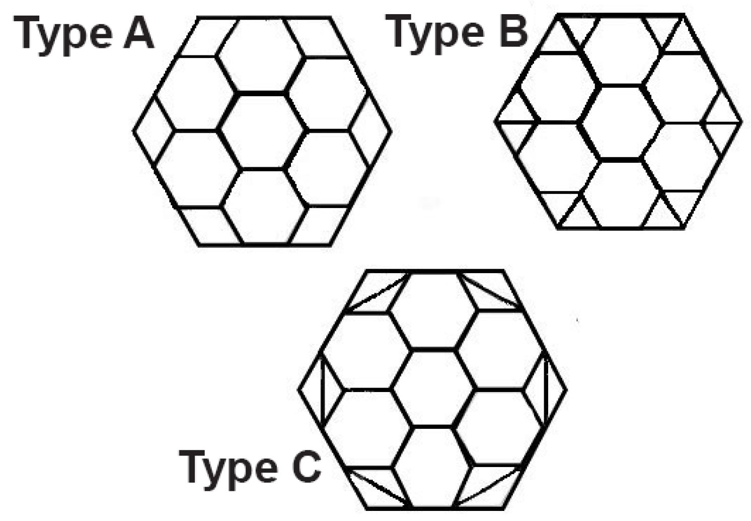
2.1. Geometrical Parameters
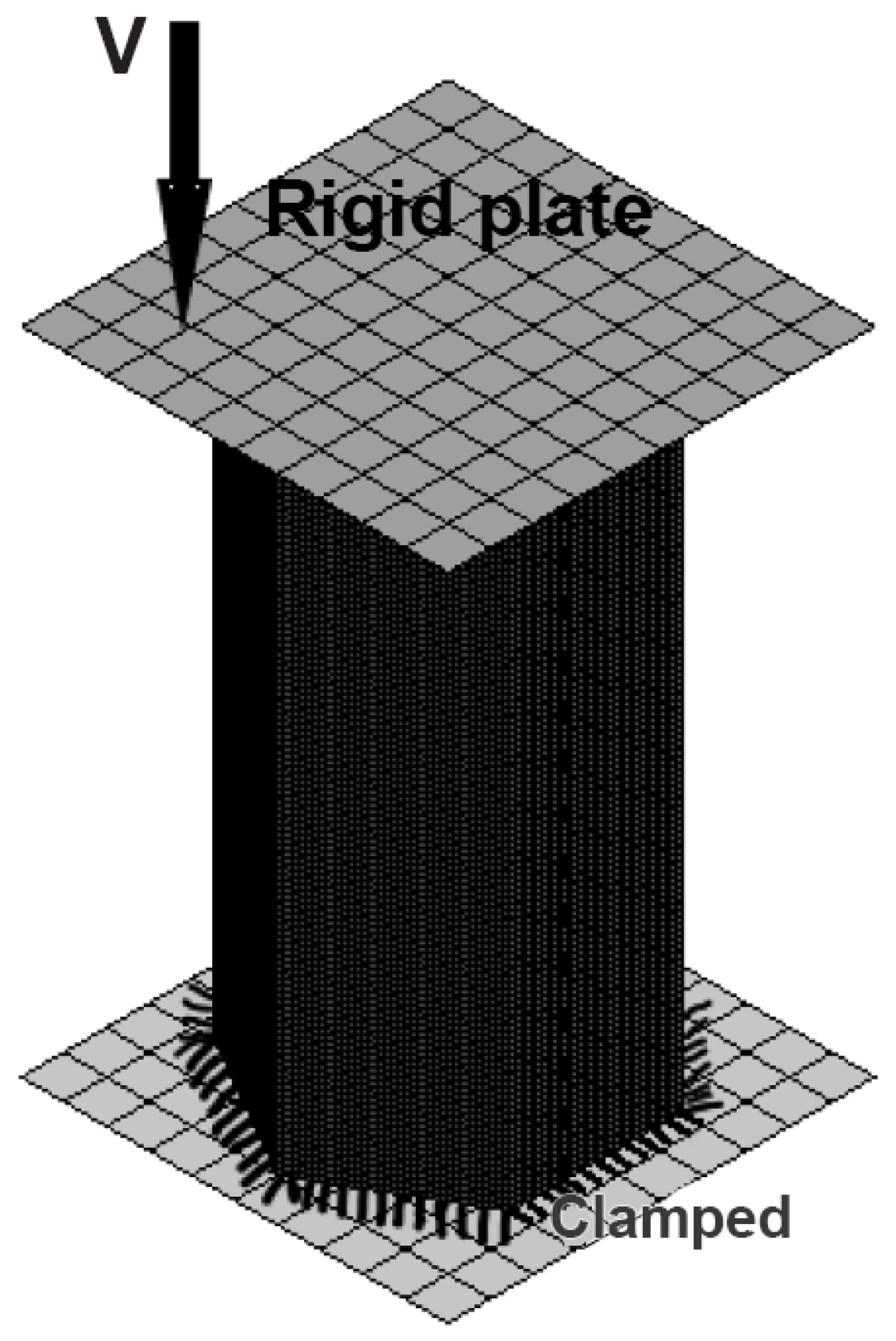
2.2. Numerical Analysis
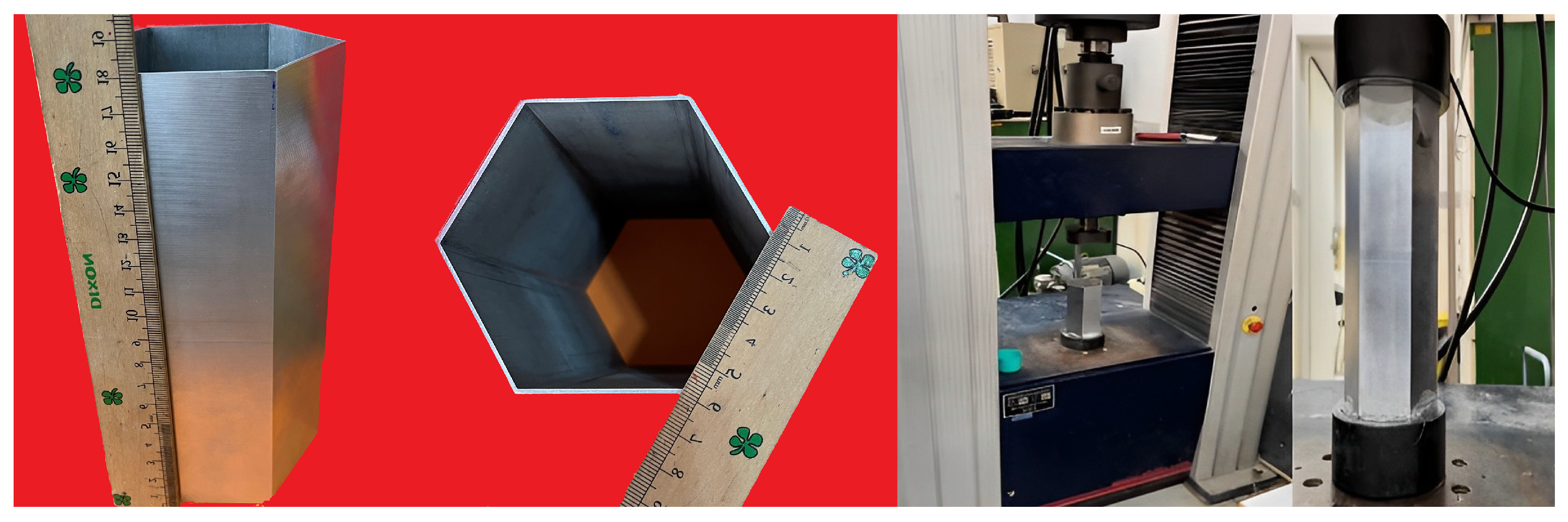
2.2.1. Model Properties and Verification
2.2.2. Definition of Crashworthiness Indicators
3. Selecting the Applicable Multi-Cell Tube with the SAW Method Based on the Numerical Results of Different Sections of the Multi-Cell Structure under Axial Dynamic Loading
4. Optimization of the Selected Section of the Multi-Cell Hexagonal Tube with Variable Thicknesses
4.1. Problem Explanation
4.2. Regression Model
4.3. Optimization of Different Variable Thicknesses of Multi-Cell Tube under Dynamic Axial Load
4.3.1. Plan A: Optimization of Variable Thicknesses Aimed at Increasing Specific Energy Absorption and Acceptable Peak Force
4.3.2. Plan B: Optimization of Thicknesses Aimed at Crushing Force Efficiency and Acceptable Peak Force
5. Conclusions
Author Contributions
Funding
Institutional Review Board Statement
Informed Consent Statement
Data Availability Statement
Conflicts of Interest
Abbreviations
| SEA | Specific energy absorption |
| F | Average force |
| F | Peak force |
| CEF | Crushing force efficiency |
| Flow stress | |
| Yield stress | |
| Ultimate stress | |
| n | Exponent of the power law |
| S | Standard deviation |
| E | Crash energy absorbed |
| m | Mass of tube |
| B | Outer side width |
| t | Thickness |
| Effective length | |
| K | The ratio of the effective crash distance to the original length |
| Dynamic coefficient | |
| SAWM | Simple additive weighting method |
| R-sq | Relative squared error |
| p | Number of samples |
| N | Number of observations |
| AHPM | Analytic hierarchy process method |
References
- Wei, L.; Zhao, X.; Yu, Q.; Zhu, G. Quasi-static axial compressive properties and energy absorption of star-triangular auxetic honeycomb. Compos. Struct. 2021, 267, 113850. [Google Scholar] [CrossRef]
- Wang, Z.; Zhang, J.; Li, Z.; Shi, C. On the crashworthiness of bio-inspired hexagonal prismatic tubes under axial compression. Int. J. Mech. Sci. 2020, 186, 105893. [Google Scholar] [CrossRef]
- Jiang, H.; Ren, Y.; Jin, Q.; Zhu, G.; Hu, Y.; Cheng, F. Crashworthiness of novel concentric auxetic reentrant honeycomb with negative Poisson’s ratio biologically inspired by coconut palm. Thin-Walled Struct. 2020, 154, 106911. [Google Scholar] [CrossRef]
- Wang, H.; Lu, Z.; Yang, Z.; Li, X. In-plane dynamic crushing behaviors of a novel auxetic honeycomb with two plateau stress regions. Int. J. Mech. Sci. 2019, 151, 746–759. [Google Scholar] [CrossRef]
- Dong, Z.; Li, Y.; Zhao, T.; Wu, W.; Xiao, D.; Liang, J. Experimental and numerical studies on the compressive mechanical properties of the metallic auxetic reentrant honeycomb. Mater. Des. 2019, 182, 108036. [Google Scholar] [CrossRef]
- Wang, Z. Recent advances in novel metallic honeycomb structure. Compos. Part Eng. 2019, 166, 731–741. [Google Scholar] [CrossRef]
- Mirfendereski, L.; Salimi, M.; Ziaei-Rad, S. Parametric study and numerical analysis of empty and foam-filled thin-walled tubes under static and dynamic loadings. Int. J. Mech. Sci. 2008, 50, 1042–1057. [Google Scholar] [CrossRef]
- Wierzbicki, T. Crushing analysis of metal honeycombs. Int. J. Impact Eng. 1983, 1, 157–174. [Google Scholar] [CrossRef]
- Gibson, L.J.; Ashby, M.F. Cellular Solids: Structure and Properties, 2nd ed.; Cambridge University Press: Cambridge, UK, 2014; pp. 1–510. [Google Scholar] [CrossRef]
- Tran, V.X.; Hong, S.T.; Pan, J.; Tyan, T.; Prasad, P. Crush behaviors of aluminum honeycombs of different cell geometries under compression dominant combined loads. Sae Tech. Pap. 2006, 22, 73–109. [Google Scholar] [CrossRef]
- Kocabas, I.; Yilmaz, H. Crashworthiness Performance of Al6061 Tubes with Stiffened Quatrefoil Sections under Axial and Oblique Impact Conditions. MÜHendis Makina 2021, 63, 23–40. [Google Scholar] [CrossRef]
- Alexander, J.M. An approximate analysis of the collapse of thin cylindrical shells under axial loading. Q. J. Mech. Appl. Math. 1960, 13, 10–15. [Google Scholar] [CrossRef]
- Wierzbicki, T.; Abramowicz, W. On the Crushing Mechanics of Thin-Walled Structures. J. Appl. Mech. 1983, 50, 727–734. [Google Scholar] [CrossRef]
- Chen, W.; Wierzbicki, T. Relative merits of single-cell, multi-cell and foam-filled thin-walled structures in energy absorption. Thin-Walled Struct. 2001, 39, 287–306. [Google Scholar] [CrossRef]
- Kim, H.S. New extruded multi-cell aluminum profile for maximum crash energy absorption and weight efficiency. Thin-Walled Struct. 2002, 40, 311–327. [Google Scholar] [CrossRef]
- Zhang, X.; Cheng, G.; Zhang, H. Theoretical prediction and numerical simulation of multi-cell square thin-walled structures. Thin-Walled Struct. 2006, 44, 1185–1191. [Google Scholar] [CrossRef]
- Zhang, X.; Zhang, H. Numerical and theoretical studies on energy absorption of three-panel angle elements. Int. J. Impact Eng. 2012, 46, 23–40. [Google Scholar] [CrossRef]
- Niknejad, A.; Liaghat, G.H.; Moslemi Naeini, H.; Behravesh, A.H. A theoretical formula for predicting the instantaneous folding force of the first fold in a single cell hexagonal honeycomb under axial loading. Proc. Inst. Mech. Eng. Part J. Mech. Eng. Sci. 2010, 224, 2308–2315. [Google Scholar] [CrossRef]
- Qiu, N.; Gao, Y.; Fang, J.; Feng, Z.; Sun, G.; Li, Q. Crashworthiness analysis and design of multi-cell hexagonal columns under multiple loading cases. Finite Elem. Anal. Des. 2015, 104, 89–101. [Google Scholar] [CrossRef]
- Alavi Nia, A.; Parsapour, M. Comparative analysis of energy absorption capacity of simple and multi-cell thin-walled tubes with triangular, square, hexagonal and octagonal sections. Thin-Walled Struct. 2014, 74, 155–165. [Google Scholar] [CrossRef]
- Altin, M.; Acar, E.; Güler, M.A. Crashworthiness optimization of hierarchical hexagonal honeycombs under out-of-plane impact. Proc. Inst. Mech. Eng. Part J. Mech. Eng. Sci. 2021, 235, 963–974. [Google Scholar] [CrossRef]
- Maulud, D.; Abdulazeez, A.M. A Review on Linear Regression Comprehensive in Machine Learning. J. Appl. Sci. Technol. Trends 2020, 1, 140–147. [Google Scholar] [CrossRef]
- Ibrahim, A.; Surya, R.A. The Implementation of Simple Additive Weighting (SAW) Method in Decision Support System for the Best School Selection in Jambi. In Proceedings of the Journal of Physics: Conference Series, Bandar Lampung, Indonesia, 9–11 August 2019; IOP Publishing: Bristol, UK, 2019; Volume 1338, p. 12054. [Google Scholar] [CrossRef] [Green Version]
- Saaty, R.W. The analytic hierarchy process-what it is and how it is used. Math. Model. 1987, 9, 161–176. [Google Scholar] [CrossRef] [Green Version]
- Qiu, N.; Gao, Y.; Fang, J.; Sun, G.; Kim, N.H. Topological design of multi-cell hexagonal tubes under axial and lateral loading cases using a modified particle swarm algorithm. Appl. Math. Model. 2018, 53, 567–583. [Google Scholar] [CrossRef]
- Tran, T.; Hou, S.; Han, X.; Chau, M. Crushing analysis and numerical optimization of angle element structures under axial impact loading. Compos. Struct. 2015, 119, 422–435. [Google Scholar] [CrossRef]
- Liu, Y. Crashworthiness design of multi-corner thin-walled columns. Thin-Walled Struct. 2008, 46, 1329–1337. [Google Scholar] [CrossRef]
- Kurtaran, H.; Eskandarian, A.; Marzougui, D.; Bedewi, N.E. Crashworthiness design optimization using successive response surface approximations. Comput. Mech. 2002, 29, 409–421. [Google Scholar] [CrossRef]
- Hou, S.; Li, Q.; Long, S.; Yang, X.; Li, W. Crashworthiness design for foam filled thin-wall structures. Mater. Des. 2009, 30, 2024–2032. [Google Scholar] [CrossRef]
- Qin, R.; Zhou, J.; Chen, B. Crashworthiness Design and Multiobjective Optimization for Hexagon Honeycomb Structure with Functionally Graded Thickness. Adv. Mater. Sci. Eng. 2019, 2019, 1–13. [Google Scholar] [CrossRef]


| Crashworthiness Criteria | |||
|---|---|---|---|
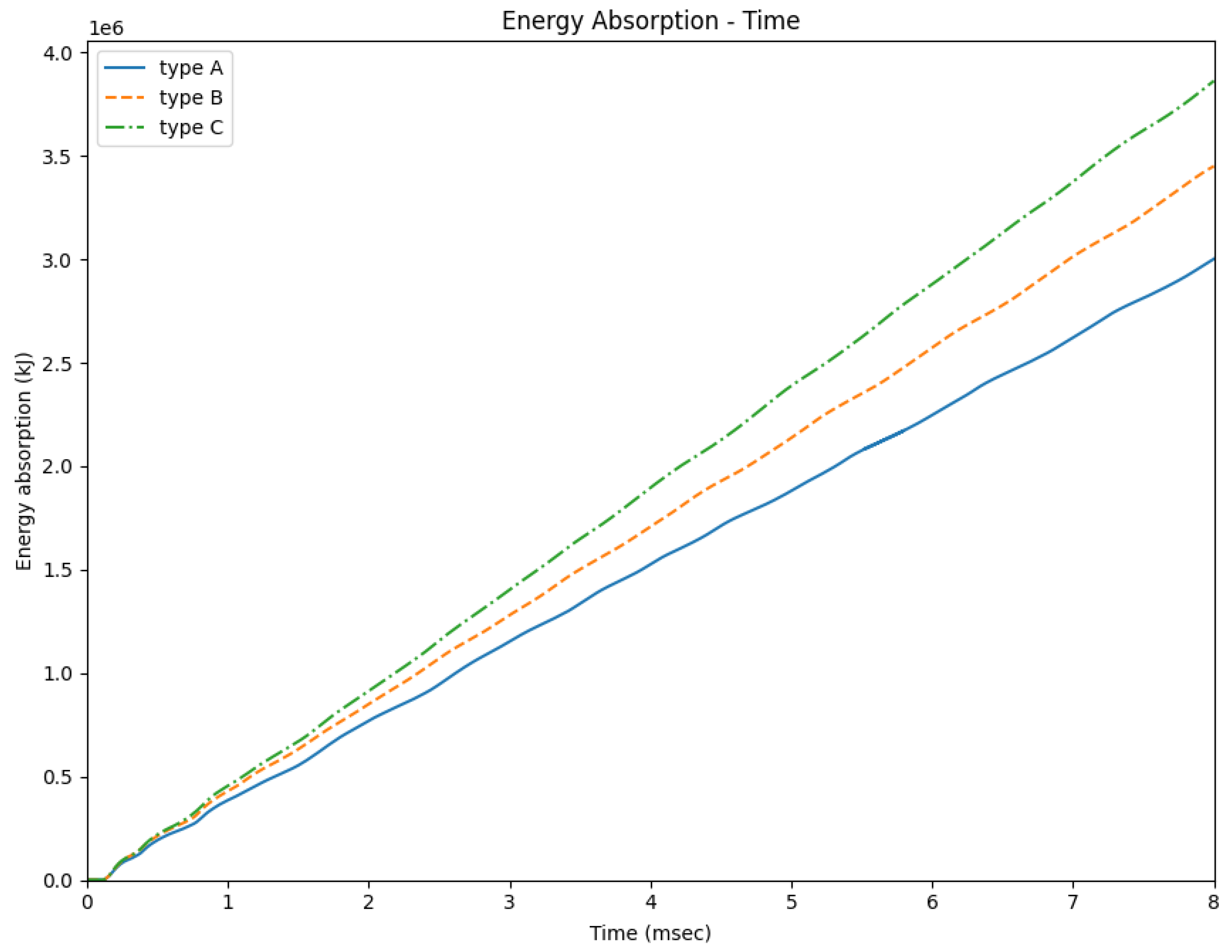
| Multi-Cell Tubes | Energy Absorption (kJ) | F (KN) | m (g) |
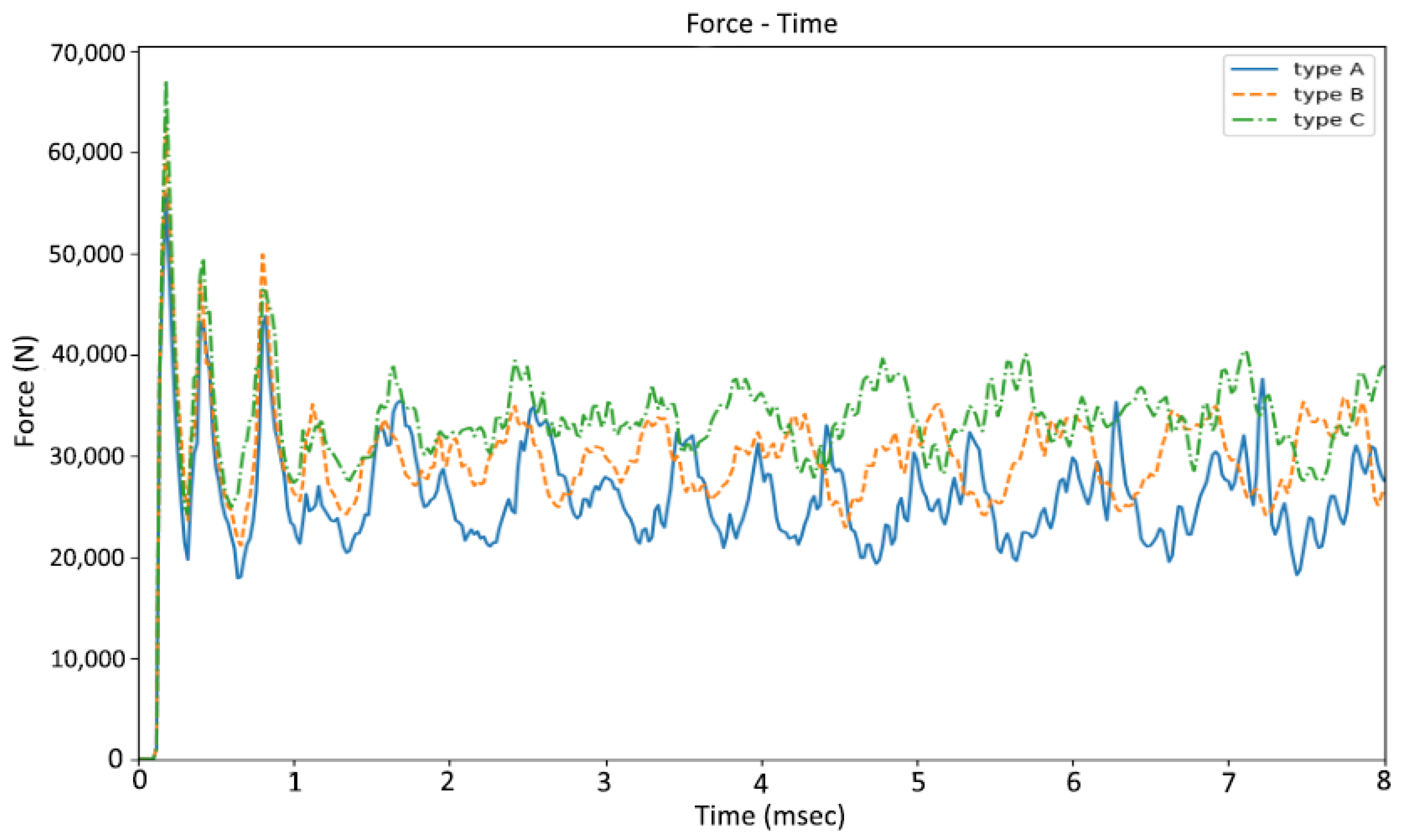
| Type A | 3.00 | 55.9 | 373.2 |
| Type B | 3.45 | 62.5 | 410.5 |
| Type C | 3.86 | 67.1 | 437.9 |
| Criteria | |||
|---|---|---|---|
| Alternative | SEA (kJ/kg) | F (KN) | CFE (%) |
| Type A | 8.04 | 55.9 | 44.7 |
| Type B | 8.40 | 62.5 | 46.0 |
| Type C | 8.81 | 67.1 | 47.9 |
| R-sq | R-sq(adj) | R-sq(pred) |
|---|---|---|
| 98.60% | 98.56% | 98.51% |
| R-sq | R-sq(adj) | R-sq(pred) |
|---|---|---|
| 97.35% | 97.28% | 97.19% |
| R-sq | R-sq(adj) | R-sq(pred) |
|---|---|---|
| 92.44% | 92.23% | 91.94% |
| R-sq | R-sq(adj) | R-sq(pred) |
|---|---|---|
| 98.99% | 98.90% | 98.70% |
| R-sq | R-sq(adj) | R-sq(pred) |
|---|---|---|
| 98.98% | 98.90% | 98.77% |
| R-sq | R-sq(adj) | R-sq(pred) |
|---|---|---|
| 95.93% | 95.65% | 95.25% |
| R-sq | R-sq(adj) | R-sq(pred) |
|---|---|---|
| 99.67% | 99.62% | 99.52% |
| R-sq | R-sq(adj) | R-sq(pred) |
|---|---|---|
| 99.11% | 98.99% | 98.84% |
| R-sq | R-sq(adj) | R-sq(pred) |
|---|---|---|
| 96.15% | 95.79% | 95.35% |
| (mm) | (mm) | (mm) | (mm) | SEA (kJ/kg) Regression Fit | SEA (kJ/kg) FEA | F (KN) Regression Fit | F (KN) FEA | RE% SEA | RE% F |
|---|---|---|---|---|---|---|---|---|---|
| 2.000 | 0.509 | 0.917 | 1.000 | 9.6195 | 9.6017 | 69.4620 | 69.1405 | 0.18 | 0.46 |
| 2.000 | 0.497 | 0.939 | 1.000 | 9.6074 | 9.5903 | 69.3011 | 69.1555 | 0.17 | 0.21 |
| 2.000 | 0.477 | 0.971 | 1.000 | 9.5834 | 9.5767 | 69.9984 | 69.1717 | 0.07 | 1.19 |
| 1.963 | 0.503 | 1.000 | 1.000 | 9.6226 | 9.5714 | 69.4978 | 69.1585 | 0.53 | 0.49 |
| 2.000 | 0.703 | 0.479 | 0.987 | 9.6964 | 9.5296 | 69.7429 | 69.5311 | 0.73 | 0.65 |
| (mm) | (mm) | (mm) | (mm) | CFE% Regression Fit | E (kJ) FEA | F (KN) FEA | F (KN) FEA | F Regression Fit | RE% F | RE% SEA | RE% CFE |
|---|---|---|---|---|---|---|---|---|---|---|---|
| 2.000 | 0.533 | 0.400 | 1.000 | 61.096 | 4.5958 | 38.2983 | 62.7766 | 61.007 | 63.8385 | 1.69 | 0.14 |
| 1.958 | 0.400 | 0.400 | 0.951 | 58.919 | 4.3417 | 36.1808 | 61.2506 | 59.070 | 61.7969 | 0.89 | 2.20 |
| 2.000 | 0.552 | 0.400 | 1.000 | 60.375 | 4.6355 | 38.6292 | 62.9961 | 61.320 | 64.2649 | 2.01 | 1.54 |
| 1.958 | 0.400 | 0.495 | 1.000 | 58.803 | 4.1303 | 34.4189 | 59.6518 | 57.695 | 62.4254 | 4.65 | 1.92 |
Disclaimer/Publisher’s Note: The statements, opinions and data contained in all publications are solely those of the individual author(s) and contributor(s) and not of MDPI and/or the editor(s). MDPI and/or the editor(s) disclaim responsibility for any injury to people or property resulting from any ideas, methods, instructions or products referred to in the content. |
© 2023 by the authors. Licensee MDPI, Basel, Switzerland. This article is an open access article distributed under the terms and conditions of the Creative Commons Attribution (CC BY) license (https://creativecommons.org/licenses/by/4.0/).
Share and Cite
Sistani, R.; Mousavi Mashhadi, M.; Mohammadi, Y. Improvement of Crashworthiness Indicators with a New Idea in the Design of the Multi-Cell Hexagonal Tube under Dynamic Axial Load. Machines 2023, 11, 641. https://doi.org/10.3390/machines11060641
Sistani R, Mousavi Mashhadi M, Mohammadi Y. Improvement of Crashworthiness Indicators with a New Idea in the Design of the Multi-Cell Hexagonal Tube under Dynamic Axial Load. Machines. 2023; 11(6):641. https://doi.org/10.3390/machines11060641
Chicago/Turabian StyleSistani, Reza, Mahmoud Mousavi Mashhadi, and Younes Mohammadi. 2023. "Improvement of Crashworthiness Indicators with a New Idea in the Design of the Multi-Cell Hexagonal Tube under Dynamic Axial Load" Machines 11, no. 6: 641. https://doi.org/10.3390/machines11060641