Article

Optimal Coordinated Control of Active Front Steering and Direct Yaw Moment for Distributed Drive Electric Bus

1
College of Mechanical Engineering and Automation, Huaqiao University, Xiamen 361021, China
2
Xiamen King Long United Automotive Industry Company, Xiamen 361006, China
*
Author to whom correspondence should be addressed.
Machines 2023, 11(6), 640; https://doi.org/10.3390/machines11060640
Submission received: 17 May 2023 / Revised: 30 May 2023 / Accepted: 31 May 2023 / Published: 11 June 2023
(This article belongs to the Special Issue Advanced Modeling, Analysis and Control for Electrified Vehicles)

Abstract

:
This paper suggests a hierarchical coordination control strategy to enhance the stability of distributed drive electric bus. First, an observer based on sliding mode observer (SMO) and adaptive neural fuzzy inference system (ANFIS) was designed to estimate the vehicle state parameters. Then the upper layer of the strategy primarily focuses on coordinating active front steering (AFS) and direct yaw moment control (DYC). The phase plane method is utilized in this layer to provide an assessment basis for the switching control safety of AFS and DYC. The lower layer of the strategy designs an integral terminal sliding mode controller (ITSMC) and a non-singular fast terminal sliding mode controller (NFTSMC) to obtain the optimal additional front wheel steering angle to improve handling performance. A fuzzy sliding mode controller (FSMC) is also proposed to obtain additional yaw moment to ameliorate yaw stability. Finally, the strategy proposed in this paper is subjected to simulation testing and compared with the performance of AFS and DYC systems. The proposed strategy is also evaluated for tracking errors in sideslip angle and yaw rate under two conditions. The results demonstrate that the proposed strategy can effectively adapt to various extreme environments and improve the maneuvering and yaw stability of the bus.

1. Introduction

As electric vehicle technology continues to advance and gain popularity, distributed drive electric bus is increasingly used in urban public transport. It offers numerous benefits such as being environmentally friendly and providing convenient dynamic control. Advancements in automotive technology have brought about significant improvements in driving safety and handling stability. However, these technological advancements have also led to an increase in security concerns. To address these concerns, many active safety control (ASC) systems [1,2,3,4] have been developed and improved to assist drivers in navigating complex and unpredictable driving conditions.
In practice, to better study the steering stability performance of vehicles, some state parameters are expensive to measure or are susceptible to environmental noise during measurement, resulting in low measurement accuracy, such as speed, sideslip angle, etc. Therefore, a large amount of observation theory has been applied to vehicle state estimation [5,6,7]. The most commonly employed methods are extended Kalman filtering (EKF), SMO, and other nonlinear observers. Fuzzy logic algorithms and neural networks have also been used in some cases. Zhang et al. proposed an integrated scheme using a dual extended-infinite Kalman filter to estimate vehicle velocity, yaw rate, and sideslip angle [8].
SMO has the advantages of simple design and high robustness in modeling errors and measurement noise. However, their performance may be compromised when dealing with nonlinear systems and in the presence of large measurement errors. To solve such problems, Chen et al. reconstructed the equations of longitudinal forces by means of model decoupling and considered the effect of noise to achieve the estimation of longitudinal forces of tires with insufficient sensor information [9]. Melzi et al. proposed a hierarchical neural network approach to estimate sideslip angle. The design of the neural network was obtained by numerical simulation of a vehicle model. Finally, post-processing of the experimental data obtained from the vehicle is performed by using an instrument [10].
Considering the deficiency of the SMO in observing the nonlinear system, ANFIS is introduced for estimating speed and sideslip angle based on the SMO in order to improve the observation accuracy in this paper.
ASC systems are designed to effectively enhance the stability and safety of vehicles on the road by means such as active steering (AS), active suspension system, DYC, etc. An AFS system has a significant impact on the lateral performance of the vehicle. When the tire force is in the linear region, lateral force does not reach saturation, and AFS performs well. However, due to the nonlinear characteristics of tire force, the performance of AFS is limited to the linear region of lateral tire force. To address this limitation, DYC can be employed to enhance the effectiveness of the vehicle control system in the non-linear region of tire dynamics. DYC is capable of improving the vehicle’s control system in both the linear and non-linear regions of tire dynamics. This makes DYC an efficient solution to overcome the limitations of AFS [11,12,13].
Although corrective yaw moments can help improve vehicle stability, they are often seen as a costly control input that should be minimized. This is because these moments are typically generated by applying braking force, which not only slows the vehicle down but can also shorten the lifespan of the tires. As a result, it is important to minimize the impact of corrective yaw moments on the vehicle’s speed and tire wear. Integrating and coordinating DYC and AFS is a useful approach to limit the excessive use of external yaw moment while maintaining stability [14,15,16]. To further improve the maneuvering and yaw stability of the vehicle, researchers have employed a variety of control algorithms such as sliding mode control (SMC) [17,18], fuzzy logic control [19], optimal control [20,21], model predictive control [22,23], and so on.
The coordinated control of AFS and DYC should take into account the maneuvering and yaw stability of the vehicle at the same time. Moreover, the control system should address uncertainties in parameters, unknown external disturbances, and non-linearity of tires. Researchers have proposed various solutions to tackle these issues [24]. Ahmadian et al. developed an adaptive coordinated control strategy for AFS and DYC. Parameter uncertainty is managed through an integrated multiple input multiple output adaptive control method of variables such as changes in vehicle mass and road adhesion coefficient. Coordinated control between AFS and DYC through a gain scheduling mechanism based on stability index [25].
Termous et al. designed a coordinated control strategy. This method coordinated AS, differential braking and active suspension through a high-order SMC and a back-stepping controller. It productively improves the handling stability, safety and ride comfort of electric vehicles [26]. Jin et al. created an integrated DYC and AFS controller based on a robust fuzzy H control strategy to improve the lateral stability and handling performance of vehicles. It applied the Takagi-Sugeno fuzzy modeling method to solve nonlinear problems of lateral dynamics of vehicles [27].
Although these methods solve some problems, they do not effectively resolve the coupling problem between maneuverability and stability, as well as the conflicts between the control objectives of various subsystems. The nonlinear coupling relationship exists in the longitudinal, lateral, and vertical directions of the vehicle, which causes many difficulties to the controller design.
Zhao et al. proposed a nonlinear SMC algorithm which realizes multi-target independent tracking and calculates the expected total body force in line with the upper-layer instructions. The actuator control layer controls the corresponding actuator to achieve optimal tire force from the body control layer [28]. Aiming at the difficulty of vehicle lateral control under high-speed conditions, Liang et al. proposed a comprehensive control method integrating AS and DYC. For light or moderate steering regions, a decoupling control method is proposed, which uses a penalty function to allocate the participation of AS and DYC for the overdrive characteristics of the vehicle. In large steering regions, based on the sideslip angle phase plane, both handling-oriented and stability-oriented controls are proposed to achieve a good balance [29].
At the same time, some articles use the phase plane method as the basis for judging vehicle yaw stability. They consider the influence of different driving conditions on the stability boundary [30,31]. Liu et al. raised a new method for establishing vehicle yaw stability criterion based on the β-r phase plane. The influence of different driving conditions (front wheel steering angle, road adhesion coefficient, and vehicle speed) on the phase plane stability boundary is emphatically analyzed, which provides a theoretical basis for the intervention of the stability control algorithm [32]. Chen et al. proposed a new extensible coordinated controller for the driving stability and handling performance of the vehicle. The controller takes into account different vehicle speeds, road adhesion coefficients, and front wheel steering angles and adopts the phase plane method to provide dynamic stability boundaries for the switching control strategies of AFS and DYC [33].
From the above studies we can learn, firstly, the coordinated control of AFS and DYC for the distributed drive electric bus is an effective mean to improve the maneuvering and yaw stability. Secondly, the controller algorithm should have good robustness and transient response characteristics to deal with the uncertainty of the vehicle state and external disturbances. Finally, the coordinated controller can operate and maintain stability depending on the different driving conditions and the stability region which the vehicle is in.
To this end, this paper designs a coordinated control mechanism of AFS and DYC for the handling and stability of distributed drive electric bus. The AFS system adopts an ITSMC and a NFTSMC to improve transient performance. The DYC system uses an FSMC to decouple the sideslip angle and yaw rate to obtain the optimal additional yaw moment and maximize the stability of the vehicle. Finally, the phase plane method is used to assess the stability region of the vehicle. A boundary layer is also set to reduce the impact of mode switching on the control system. Different control systems are implemented according to different driving conditions to improve the maneuvering and yaw stability of the bus.
The remainder of this paper consists of the following parts. Section 2 introduces the two distributed drive electric bus dynamic models. Section 3 presents the design and verification of the state observer. Section 4 expands on the design process of the hierarchical coordination controller. Section 5 simulates and verifies the designed coordination controller. Section 6 is the conclusion.

2. Vehicle System Modeling

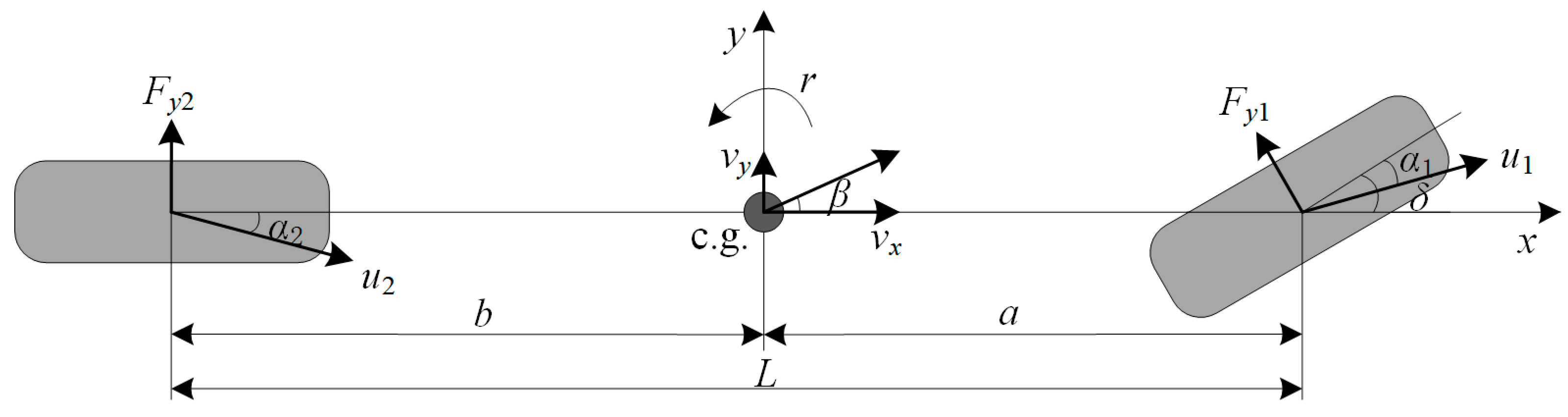
2.1. Linear 2-DOF Vehicle Model

The linear “two degrees of freedom” (2-DOF) vehicle model is called the ideal reference model. This model has many advantages, such as fewer parameters, low complexity, simple structure, and better real-time performance. It can accurately reflect the kinetic relationship between the front wheel steering angle and the sideslip angle of center of gravity and yaw rate. It plays an important role in the development of bus stability control algorithms. The force analysis is shown in Figure 1.
The model uses the front wheel steering angle as input and assumes that the vehicle is moving at a constant speed and the steering angles of the left and right sides are the same. Only the lateral motion on the horizontal plane of the vehicle and the yaw motion around the center of gravity are considered.
The dynamic equation of the body motion is as follows:
F y = m ( v x r + v x β ˙ ) = F y 1 cos δ + F y 2 M z = I z r ˙ = a F y 1 cos δ b F y 2
where m is the vehicle mass; νx is the longitudinal speed; νy is the lateral speed; r is the yaw rate; δ is the front wheel steering angle; a is the distance from the center of gravity of the vehicle to the front axle; b is the distance from the center of gravity of the vehicle to the rear axle; Iz is the yaw moment of inertia; Fyi is the lateral force of the i-th wheel (i = 1, 2); Fy is the resultant lateral force; Mz is the resultant yaw moment.
Assuming that δ is very small, the above formula can be written as:
F y = m ( v x r + v x β ˙ ) = k 1 α 1 + k 2 α 2 M z = I z r ˙ = a k 1 α 1 b k 2 α 2
where ki is the lateral tire stiffness of the i-th wheel (i = 1, 2); αi is the sideslip angle of the i-th wheel (i = 1, 2).

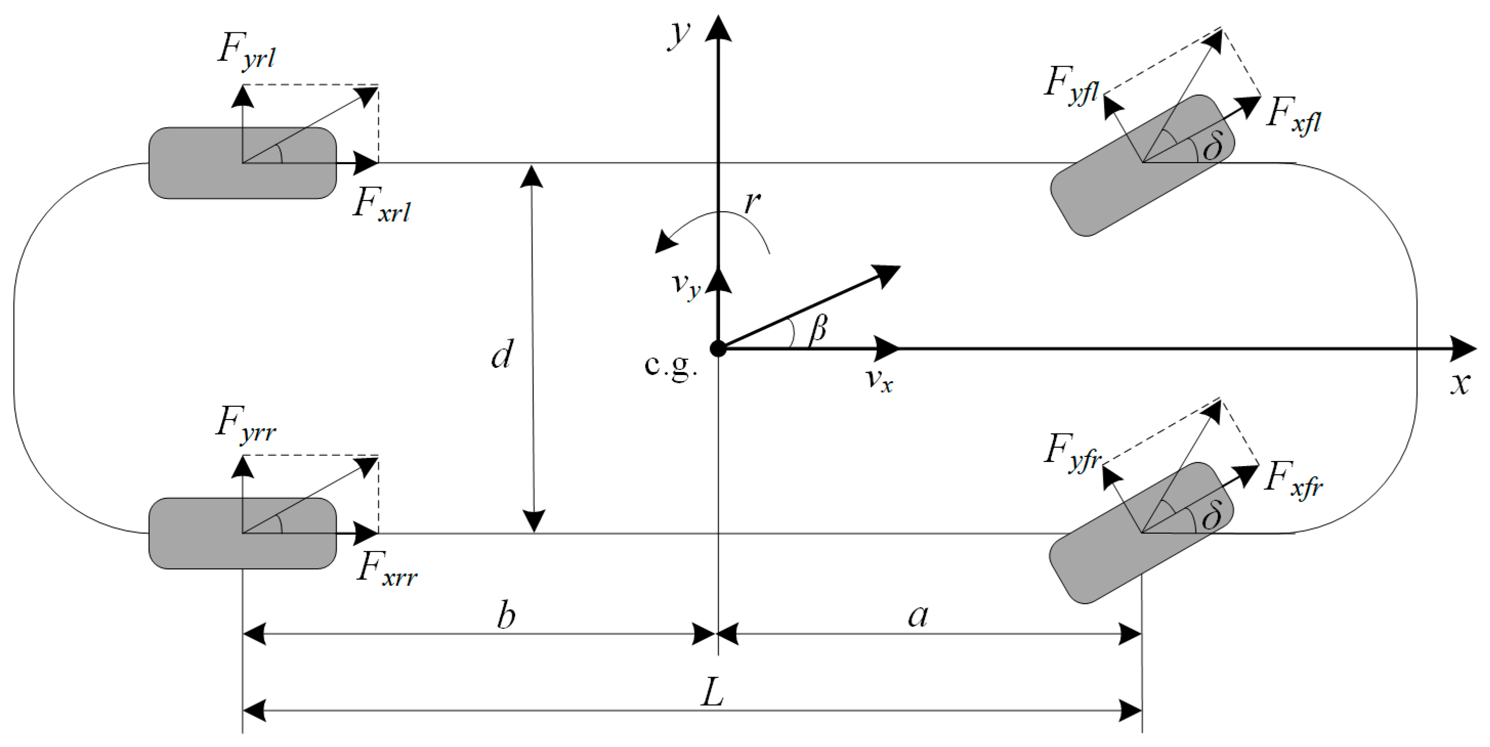
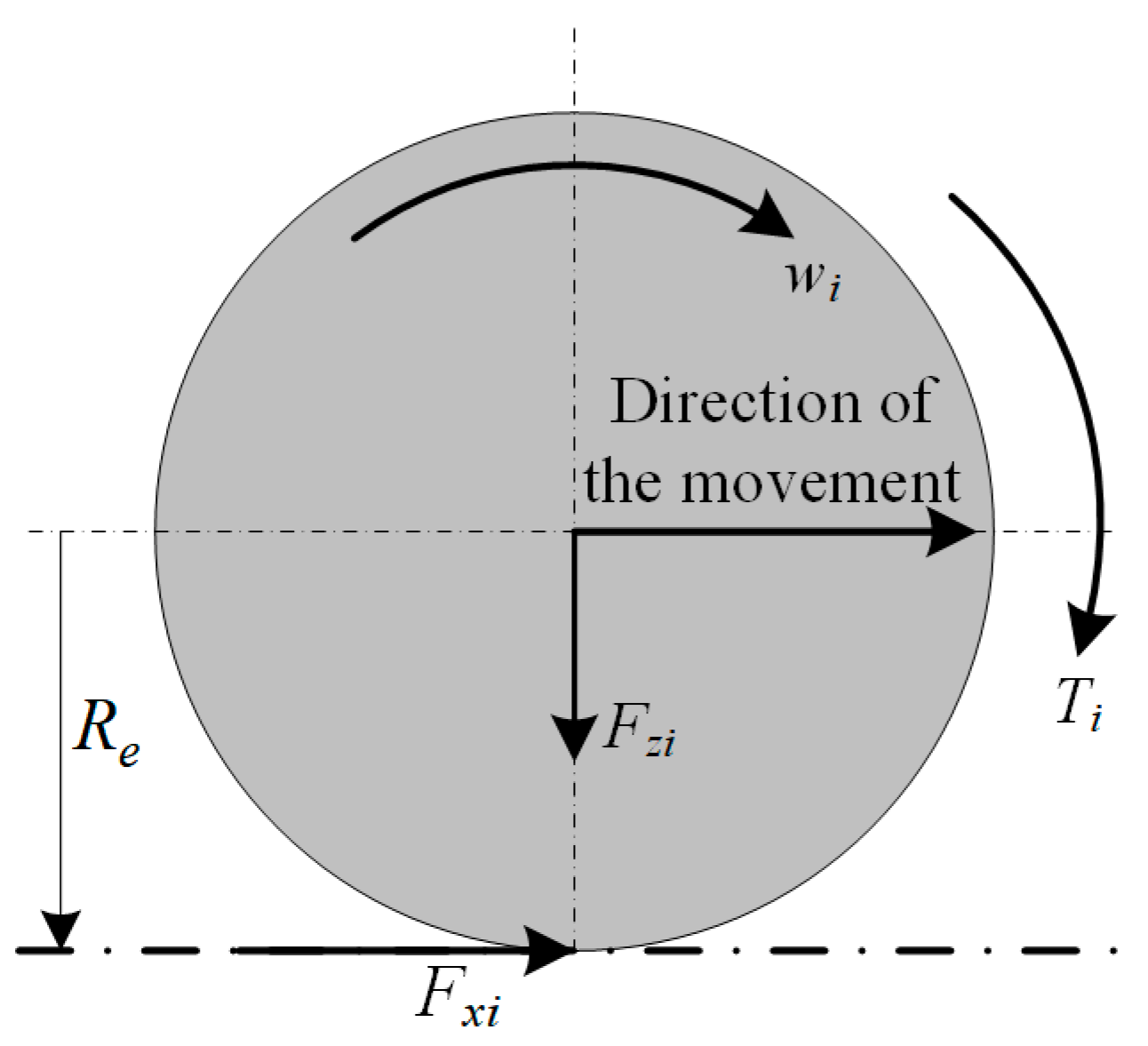
2.2. Nonlinear 7-DOF Vehicle Model
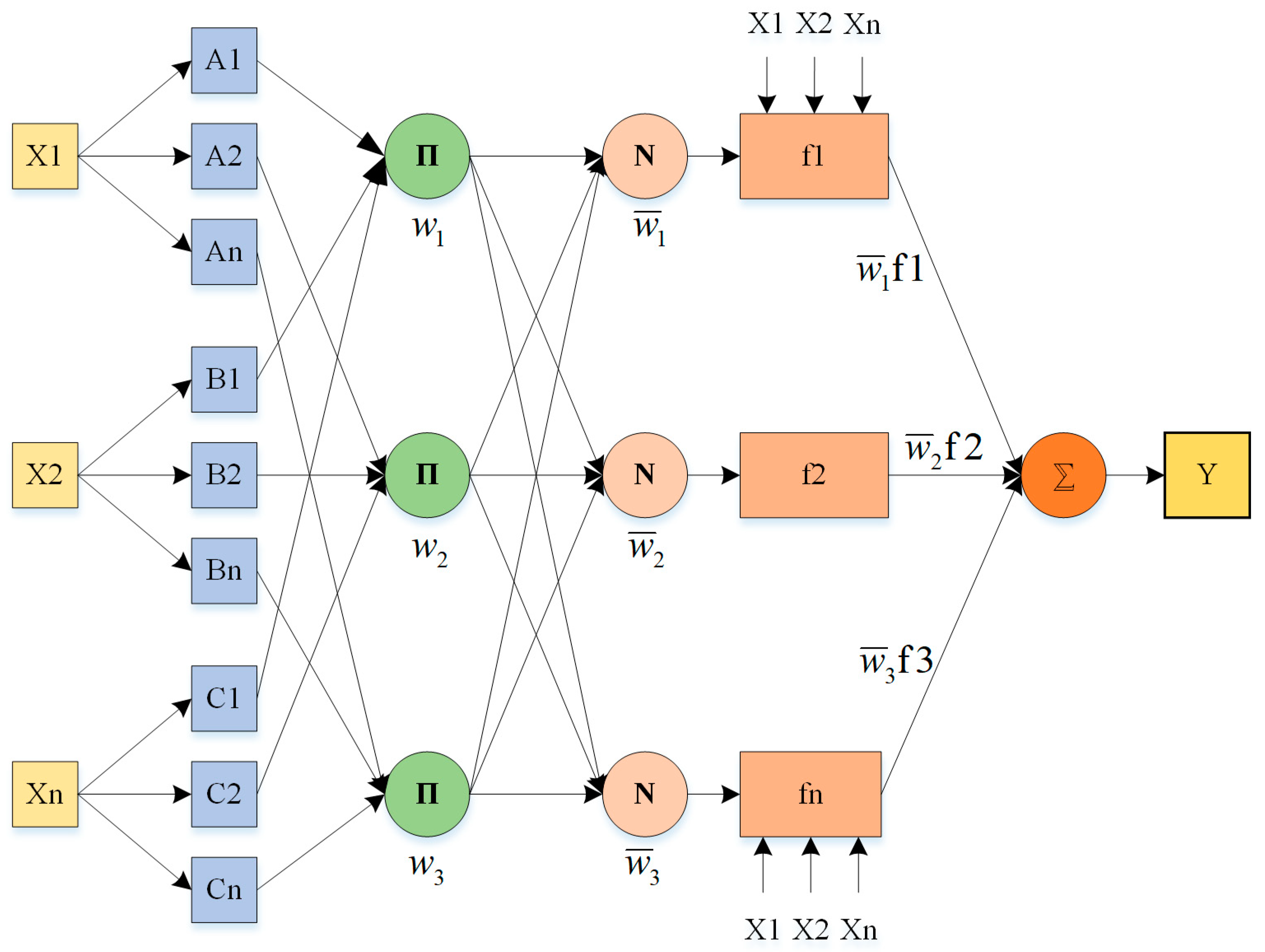
The nonlinear “seven degrees of freedom” (7-DOF) model is widely used in vehicle dynamic simulation research. It has important application value in the research and development of vehicle dynamics and can provide strong support for the evaluation and optimization of vehicle performance. The vehicle coordinate system and force analysis are shown in Figure 2.
The dynamic equation is as follows:
m ( v ˙ x v y r ) = ( F x f l + F x f r ) cos δ ( F y f l + F y f r ) sin δ + F x r l + F x r r m ( v x β ˙ + v x r ) = ( F x f l + F x f r ) sin δ + ( F y f l + F y f r ) cos δ + F y r l + F y r r I Z r ˙ = a ( F x f l + F x f r ) sin δ + a ( F y f l + F y f r ) cos δ b ( F y r l + F y r r ) d 2 ( F x f l F x f r ) cos δ + d 2 ( F y f l F y f r ) sin δ d 2 ( F x r l F x r r )
where Fxi is the longitudinal force of the each wheel (i = fl, fr, rl, rr); Fyi is the lateral force of the each wheel (i = fl, fr, rl, rr).
The force analysis of the vehicle wheels is shown in Figure 3. According to the torque balance of wheel dynamics, the wheel rotation dynamics equation can be obtained as follows:
J w w ˙ = T i F x i R e
where Jw is the wheel moment of inertia, Re is the effective radius of wheels, wi and Ti denote the angular velocity and wheel torque of the i-th wheel (i = 1, 2, 3, 4), respectively.
Only the effect of vehicle load transfer caused by vehicle longitudinal and lateral acceleration on the wheel vertical load is considered. Thus the vertical load equation for each wheel is shown in the following equation.
F z f l = 1 2 m g b L 1 2 m a x h g L m a y b L h g d F z f r = 1 2 m g b L 1 2 m a x h g L + m a y b L h g d F z r l = 1 2 m g a L 1 2 m a x h g L m a y b L h g d F z r r = 1 2 m g a L 1 2 m a x h g L + m a y b L h g d
where Fzi is the vertical force of the i-th wheel (i = 1, 2, 3, 4), hg is the height of the center of gravity.
The definitions and values of the parameters mentioned in the article are shown in Table 1:

3. State Observer

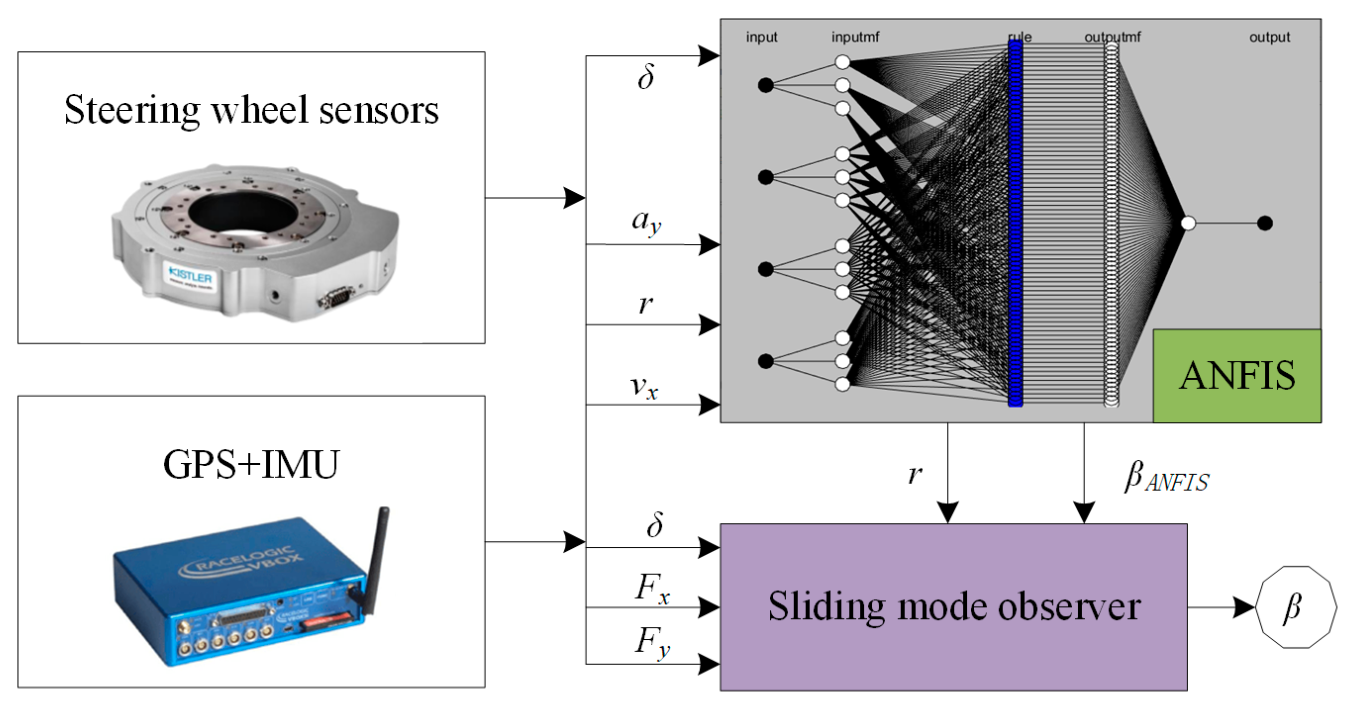
3.1. The Observer Design

Due to the limitations of the measurement position, the limited accuracy of the sensors, and the change of vehicle attitude during motion, there are many limitations and difficulties in the measurement of vehicle speed and the sideslip angle of the center of gravity, which need to be fused and derived from information from multiple sensors to improve measurement accuracy and precision.
Therefore, to address the above problems, a theory-based nonlinear sliding mode variable structure observer is proposed, based on which an ANFIS is introduced as a pre-observable quantity to effectively overcome the inherent chattering phenomenon of the sliding mode observer, the dependence on the system model, and the sensitivity to measurement noise and to improve the accuracy of the observer. The structure of the observer is shown in Figure 4.
ANFIS is an intelligent control method that combines fuzzy logic and neural networks for modeling and controlling nonlinear systems. ANFIS is capable of approximating arbitrary linear as well as nonlinear data with arbitrary accuracy. It is also characterized by high accuracy, low error, short convergence time, and few training samples required. Its activation functions include the sigmoid function, gaussian function, trapezoidal function, etc. A typical ANFIS structure is illustrated in Figure 5.
When the input variables are fuzzified, the fuzzy quantities of the output variables are generated by fuzzy rules and neural networks, and then the actual physical quantities are obtained by inverse fuzzification. The neural network is used to adjust the parameters of the fuzzy rules.
The criteria considered for input selection by ANFIS are generally the selection of the minimum number of inputs and the selection of signals that can be measured by the on-board sensors. Therefore, the following parameters are selected as inputs: wheel steering angle, lateral acceleration, yaw rate, and longitudinal speed. The output parameters are the sideslip angle. To generate the fuzzy logic estimator presented in this paper, an ANFIS toolbox for Matlab was used. The neural network was generated and trained based on the input data specified earlier.
SMO is an observer algorithm based on sliding mode control theory, the core idea of which is to achieve the estimation of the system state by introducing a sliding mode surface.
The expression for the nonlinear form of the observer is:
x ˙ = f ( x , u ) y = C x
The output vector y is a linear function of the state vector x which can be measured directly by the sensor, and u is the input variable. C is the coefficient matrix.
In the design of the sliding mode observer, it is first necessary to construct the sliding mode surface, defined as follows:
s ( x , t ) = e y = y ^ y = C ( x ^ x ) = s 1 , , s n T
When the sliding surface satisfies the sliding condition:
d d t ( 1 2 s i 2 ) η s i
η is positive value. The sliding surface will converge to zero in a finite time. When the nonlinear system is energetically observable, the system trajectory line converges to the true value in the sliding mode plane in finite time.
Therefore, the sliding mode algorithm can be described by the following equation:
x ^ ˙ = f ( x ^ , u ) H C ( x ^ x ) K sgn ( y y ^ )
The feedback gain K is introduced to control the system state estimates toward the sliding surface. K needs to be chosen according to the design of the sliding surface and the system characteristics. H is the gain matrix.
Based on the above mentioned analysis, this paper has designed an estimation methodology of bus state parameters based on SMO and ANFIS where the state vector is:
x = [ v x v y r ]
the observed vector is:
y = [ r β A N F I S ]
the input vector is:
u = [ δ F x F y ]
Therefore, the observer can be constructed as follows:
x ^ ˙ = f ( x ^ , u ) H ( r ^ r , β ^ β A N F I S ) K s a t [ ( r ^ r + β ^ β A N F I S ) / λ ]
The function sat(x) is chosen as the switching function of the sliding mode observer to reduce the chattering of the system. This is equivalent to setting the boundary layer around the sliding mode surface. λ is the thickness of the boundary layer.
The longitudinal and lateral velocities of the bus can be estimated by the above observer and then according to following equation:
β = arctan v y v x
The final sideslip angle of the center of gravity can be estimated.

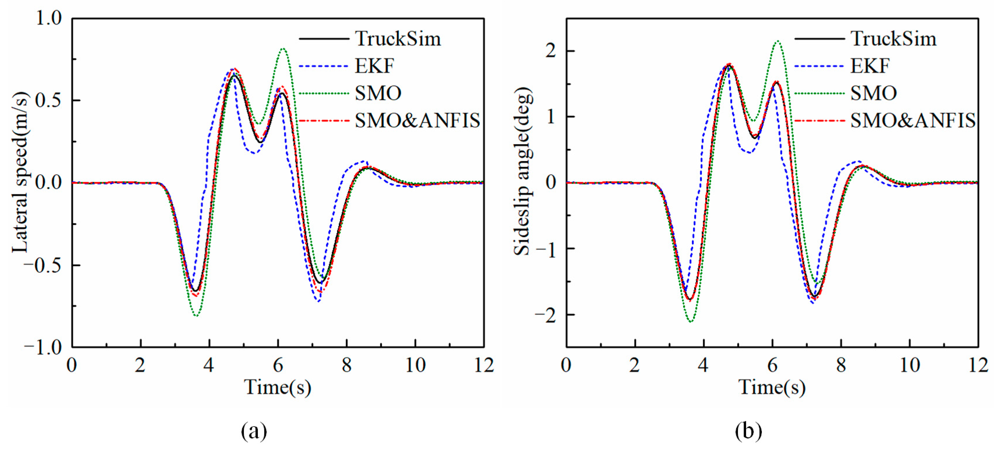
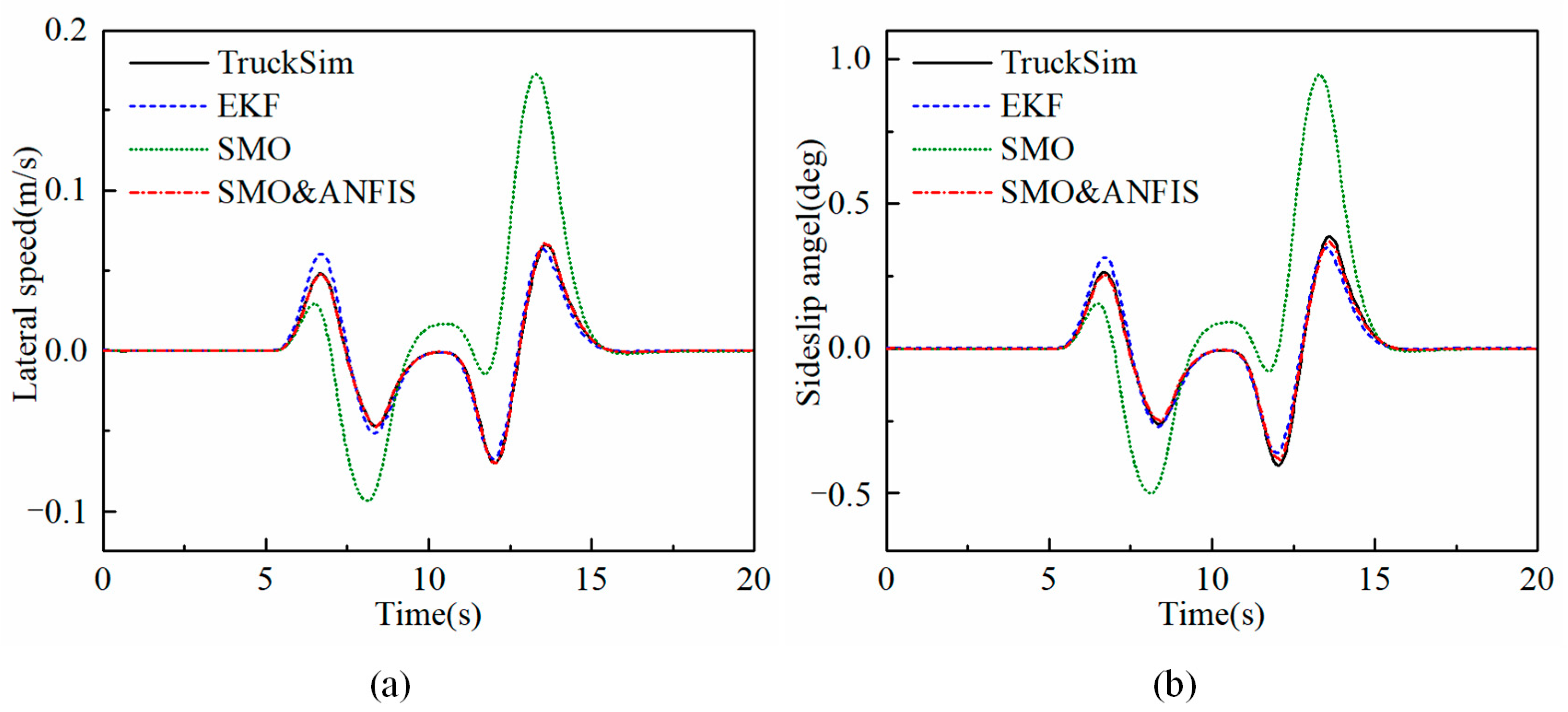
3.2. The Observer Simulation Verification

To verify the performance of the designed observer in terms of vehicle speed as well as sideslip angle, a double lane change simulation test was performed. The observer performance is also compared with that of the EKF and SMO estimation methods.
The vehicle speed is set to 80 km/h and the road adhesion coefficient is 0.85. The results are illustrated in Figure 6.
The simulation response results of the sideslip angle and the lateral speed show that the observation accuracy of the EKF is inferior to that of the SMO and SMO&ANFIS observers, in which there is always a large error, while the observation accuracy of the SMO observer suddenly deteriorates at the moment of the vehicle turning. The SMO&ANFIS observer overcomes this problem and maintains high observation accuracy throughout the observation process.
At low speed and a low adhesion coefficient, the bus speed is set to 40 km/h and the road adhesion coefficient is set to 0.5. As seen in Figure 7, by comparing the estimated results of the sideslip angle and lateral speed with the ideal values from TruckSim, it can be seen that there is a large error in the SMO, and the observation accuracy of the EKF decreases slightly at the moment of vehicle steering, which is the opposite of the high speed, high adhesion coefficient condition. In contrast, the SMO&ANFIS observer is not affected by vehicle turning conditions and maintains a high observation accuracy.

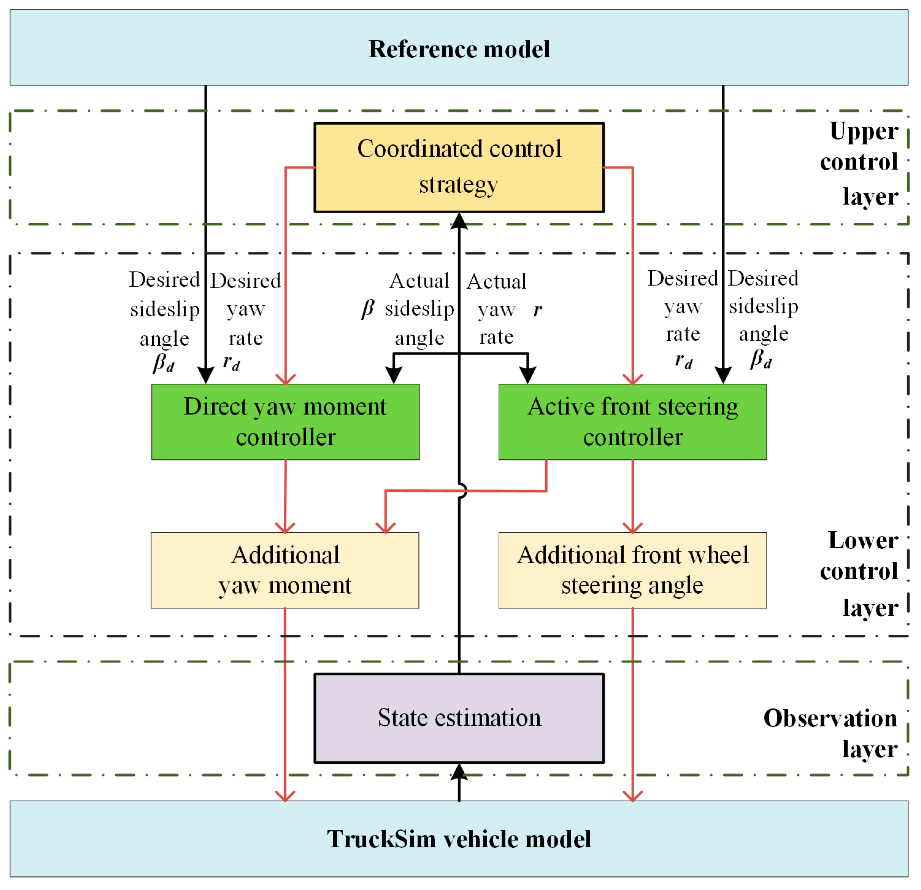
4. Hierarchical Coordinated Controller Design

The handling stability of the vehicle is mainly determined by the lateral and longitudinal force characteristics of the tires. AFS and DYC are both designed to change the lateral and longitudinal force of the tires, so that the vehicle handles according to the driver’s manipulation intention. However, the longitudinal and lateral force of the tires have serious coupling and are limited by the road adhesion coefficient. An important issue in vehicle dynamics control research has been how to reasonably adjust the force state of the tires so that the AFS and DYC systems can generate their respective optimal effects.

4.1. AFS Controller Design for Handling

4.1.1. Sideslip Angle Controller

According to Equation (1), the sideslip angle β follows a first-order dynamic system with respect to the lateral tire force Fy. Therefore, the ITSMC method can be employed to minimize sideslip angle.
The state variables of the system can be set as:
x 1 = e β = β β d x 2 = x ˙ 1 = e ˙ β = β ˙ β ˙ d
The sliding surface of the ITSMC controller can be selected as:
s β = e β + 0 t ( α β 2 e β + β β 2 γ β e β γ β ) d t
By the formula in Equation (1):
e ˙ β = r + F y m v x + g β
gβ is an unknown but bounded function. It is used to represent uncertainty and disturbance in practical nonlinear vehicle models and defined as:
| g β | k β , k β > 0
Therefore, assuming Fy as the control output, we can obtain:
F y = m v x [ α β 2 e β + β β 2 γ β e β γ β r + α β 2 s β + β β 2 sgn ( s β ) + k β sgn ( s β ) ]
Proof: 
According to the Lyapunov function definition:
V 1 = 1 2 s β 2
Differentiating V1 with respect to time:
V ˙ 1 = s β s ˙ β = s β ( e ˙ β + 1 2 α β e β + β β 2 γ β e β γ β ) = s β ( r + F y m v x + g β + α β 2 e β + β β 2 e β γ β )
According to Equation (19), we can obtain:
V ˙ 1 = k β | s β | + g β s β α β 2 s β 2 β β 2 | s β | k β | s β | + | g β | | s β | α β 2 s β 2 β β 2 | s β |
Through Equation (18), we can obtain:
V ˙ 1 α β 2 s β 2 β β 2 | s β | α β V 1 β β V 1 1 2 0
It can be demonstrated that the system can converge in a short finite time on ITSMC surfaces. □
Finally, the front wheel steering angle of the sideslip angle controller can be derived:
δ β = 1 k 1 [ F y ( k 1 + k 2 ) β a k 1 b k 2 v x r ]

4.1.2. Yaw Rate Controller

According to Equation (1), the vehicle yaw angle ψ follows the second-order dynamic system with respect to the yaw moment Mz. The NFTSMC method can be used to design the yaw rate controller.
The state variables of the system can be set as:
x 1 = e ψ = ψ ψ d x 2 = x ˙ 1 = e ˙ ψ = e r = r r d
The sliding surface of the NFTSMC controller can be defined as:
s ψ = e ψ + α ψ | e ψ | γ ψ 1 sgn ( e ψ ) + β ψ | e ˙ ψ | γ ψ 2 sgn ( e ˙ ψ )
Equation (1) can be converted into:
e ˙ r = e ¨ ψ = 1 I z M A F S + g ψ
MAFS is an additional yaw moment that improves vehicle handling stability. gψ is an unknown but bounded function which satisfies the following equation.
| g ψ | k ψ 1 , k ψ 1 > 0
Therefore, MAFS as a control input can be obtained thus:
M A F S = I z [ 1 β ψ γ ψ 2 | e ˙ ψ | 2 γ ψ 2 sgn ( e ˙ ψ ) ( 1 + α ψ γ ψ 1 | e ψ | γ ψ 1 1 ) + k ψ 1 sgn ( s ψ ) + k ψ 2 s ψ ]
Proof: 
According to the Lyapunov function definition:
V 2 = 1 2 s ψ 2
Differentiating V2 with respect to time:
V ˙ 2 = s ψ s ˙ ψ = s ψ ( e ˙ ψ + α ψ γ ψ 1 | e ψ | γ ψ 1 1 e ˙ ψ + β ψ γ ψ 2 | e ˙ ψ | γ ψ 2 1 e ¨ ψ )
Substituting Equations (27) and (29) into Equation (31) obtains:
V ˙ 2 = s ψ ( β ψ γ ψ 2 | e ˙ ψ | γ ψ 2 1 g ψ k ψ 1 β ψ γ ψ 2 | e ˙ ψ | γ ψ 2 1 sgn ( s ψ ) k ψ 2 β ψ γ ψ 2 | e ˙ ψ | γ ψ 2 1 s ψ )
Through Equation (28), it can be concluded that:
V ˙ 2 k ψ 2 β ψ γ ψ 2 | e ˙ ψ | γ ψ 2 1 s ψ 2 2 k ψ 2 β ψ γ ψ 2 | e ˙ ψ | γ ψ 2 1 V 2 0
The system can satisfy the Lyapunov stability condition, and the system state will reach the NFTSMC surface in a short finite time. □
Finally, the front wheel steering angle of the yaw rate controller can be derived as:
δ ψ = 1 a k 1 [ M A F S ( a k 1 b k 2 ) β a 2 k 1 b 2 k 2 v x ]
The final front wheel steering angle generated by the AFS system is the combination of the two controllers. The final additional front wheel steering angle is:
δ = w 1 δ β + w 2 δ ψ
where w1 and w2 are weighting coefficients.
The optimal value is obtained through continuous experiments.

4.2. DYC Controller Design for Stability

4.2.1. Adaptive Fuzzy Sliding Mode Controller

In this paper, an adaptive fuzzy sliding mode control method is proposed to adjust the coupling relationship between the sideslip angle and the yaw rate in real time, so as to improve the performance of the control system and meet the actual needs. The state variables of the system can be set as:
x 1 = e = λ ( β β d ) + ( 1 λ ) ( ψ ψ d ) x 2 = x ˙ 1 = e ˙ = λ ( β ˙ β ˙ d ) + ( 1 λ ) ( r r d )
λ represents the control weight factor between sideslip angle and yaw rate, 0 < λ < 1.
The sliding surface function is defined as:
s = k 1 e + k 2 e ˙
where k1 > 0, k2 > 0.
The yaw motion balance equation is transformed into the following equation:
r ˙ = 1 I Z [ M Z + P ]
where P express as:
P = a ( F x f l + F x f r ) sin δ + a ( F y f l + F y f r ) cos δ b ( F y r l + F y r r ) + d 2 ( F y f l F y f r ) d 2 ( F x f l F x f r ) cos δ d 2 ( F x r l F x r r )
The final control law of DYC can be obtained:
M D Y C = I Z 1 λ [ k 1 k 2 e ˙ λ ( β ¨ β ¨ d ) + ( 1 λ ) r ˙ d η sgn ( s ) ] P
where η is a positive constant (η > 0).
Proof: 
According to the definition of the Lyapunov function:
V = 1 2 s 2
The formula is obtained by deriving it with respect to time:
V ˙ = s s ˙ = s { k 1 e + k 2 { λ ( β ¨ β ¨ d ) + ( 1 λ ) [ 1 I Z ( M D Y C + P r ˙ d ) ] } }
By substituting Equation (40) into Equation (42), finally the following value is obtained:
V ˙ = s [ η sgn ( s ) ] = η | s | < 0
According to the above proof, the system state can eventually converge along the sliding mode surface, and the designed controller will eventually tend to be stable. □
This paper designs a variable weight coefficient. Using fuzzy control, the weight coefficient is adjusted according to the tracking error of the sideslip angle and yaw angle. eβ and eψ are respectively used as the fuzzy control inputs, and the weight coefficient λ is used as the fuzzy control output, shown in Table 2.

4.2.2. Torque Distribution Controller

The additional yaw moment calculated by the current controller requires a reasonable distribution method to distribute it to each wheel in order to obtain a good control effect. Therefore, this paper proposes a torque distribution method based on the dynamic load in the vertical direction of the wheel. The longitudinal force obtained from the controllers needs to be distributed according to the vertical load of each wheel. In this case, the individual longitudinal force of each tire can be effectively used. From the above, we can obtain
c l = F x f l / F x r l = F z f l / F z r l c r = F x f r / F x r r = F z f r / F z r r
where cl and cr are the ratio of the vertical load on the left wheel and the ratio of the vertical load on the right wheel.
The total longitudinal force and yaw moment of the vehicle are:
F x = F x f l cos δ + F x f r cos δ + F x r l + F x r r M Z = d 2 ( F x f r F x f l ) cos δ + d 2 ( F x r r F x r l )
According to Equations (37) and (38), we can obtain:
F x f l = 1 cos δ + 1 / c l ( F x 2 M Z d ) F x f r = 1 cos δ + 1 / c r ( F x 2 + M Z d ) F x r l = 1 c l cos δ + 1 ( F x 2 M Z d ) F x r r = 1 c r cos δ + 1 ( F x 2 + M Z d )
The longitudinal force of each wheel is obtained. Finally, according to the tire radius, the additional moment of each wheel can be obtained.

4.3. Coordinated Controller Design

4.3.1. Overall Structure of the Coordinated Controller

AFS and DYC control systems have their own advantages and disadvantages and complement each other. Adjusting the steering angle changes the lateral force and also directly affects the longitudinal force margin. Therefore, it is necessary to coordinately control the AFS and DYC systems to achieve the best utilization effect of tire force and better ensure the safety and stability of the vehicle. The overall structure diagram is shown in Figure 8.
Taking the linear 2-DOF model as the reference model, the desired sideslip angle and desired yaw rate are obtained. Then, through the AFS and DYC systems, the additional yaw moment and additional front wheel steering angle needed to maintain vehicle stability are obtained. The key to the coordinated control strategy lies in the distribution and coordination between the two systems. Therefore, it is necessary to improve the identification and assessment of the working conditions of the two systems and reduce the occurrence of incorrect assessment. On this basis, an assessment method based on the phase plane method was designed, namely an allocation algorithm for calculating the respective weight coefficients of AFS and DYC by determining vehicle state. The purpose of this is to divide the respective working areas of the two systems, taking into account vehicle handling and yaw stability.

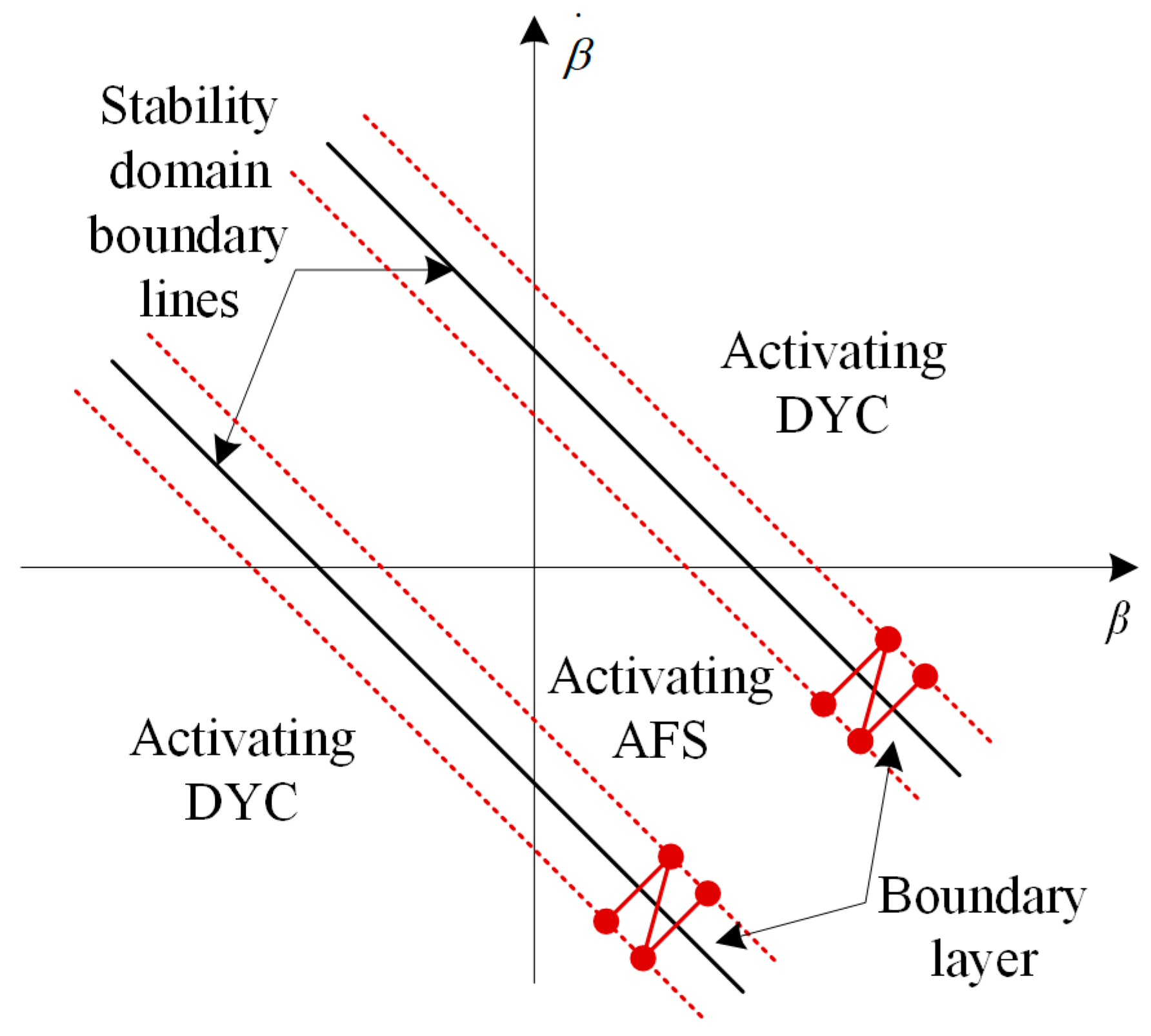
4.3.2. Determination of the Stability Boundary

In the AFS control system, the stability of the vehicle is maintained by adjusting the lateral force between the tire and the ground. In the DYC control system, the yaw movement of the vehicle is corrected by controlling longitudinal force to ensure the stability of the vehicle. Therefore, it is very important to correctly identify the state of the vehicle and determine whether it is in the stable or unstable zone.
The phase plane method is a commonly used method for judging vehicle instability. In the phase plane model, when the vehicle exits the stable domain, it means that the vehicle loses stability, and corresponding control is required to correct the vehicle’s state and restore its stability.
The double line method is one of the stable domain division methods shown in Figure 9. When the trajectory of the vehicle is outside the two boundary lines, the vehicle enters an unstable region, and stability control is required. This method can determine the stability of the vehicle more accurately, and the calculation is simple and easy to implement.
This paper uses the phase plane method of the sideslip angle and the sideslip angle rate. The assessment formula used in this paper is as follows:
χ = | 1 24 β + 4 24 β ˙ |
where χ is the stability index. When the vehicle is in the stable area, it is necessary to activate AFS and deactivate DYC. When the vehicle state is outside the demarcation lines, AFS needs to be deactivated and DYC is activated

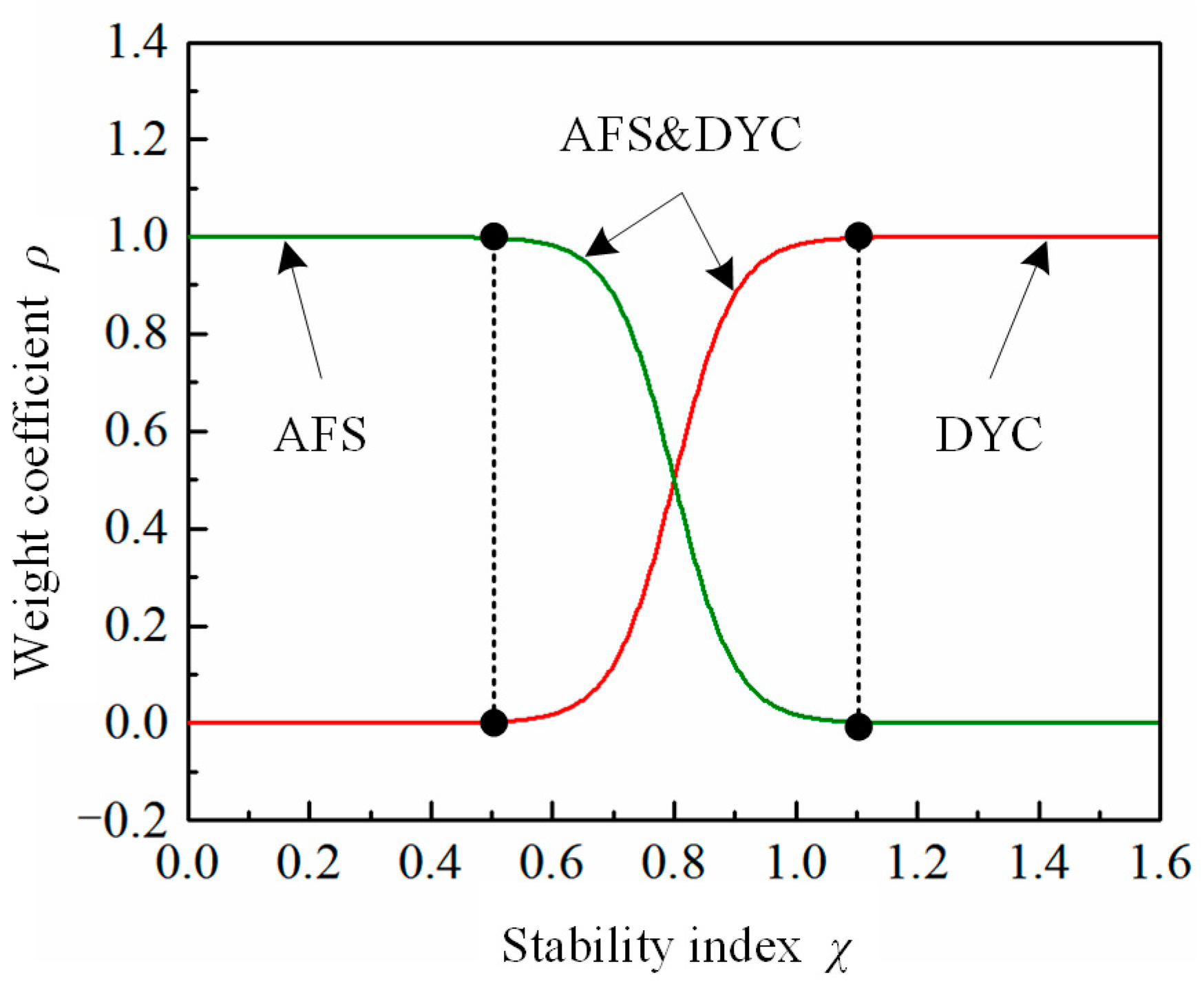
4.3.3. Distribution of Additional Yaw Moment

The vehicle will switch back and forth between AFS and DYC near the boundary line of the stable area. Mode switching will cause frequent switching of actuators. In order to reduce this effect, a boundary layer can be added near the boundary line shown in Figure 9. When the vehicle state is in the boundary layer, AFS and DYC are activated simultaneously, and the additional yaw moment of the two is distributed by distribution coefficient ρ. Therefore, the final body yaw moment is calculated as follows:
M = ρ M A F S + ( 1 ρ ) M D Y C
where M is the final required yaw moment. ρ is the weight coefficient between the AFS and DYC systems. It can be obtained from the following equation:
ρ = 1 1 + e ( χ a ) b
where a is the threshold value taken as 0.8 and b is a constant taken as 20, which controls the switching speed of the function.
Then the relationship between the stability index χ and the weight coefficient ρ are shown in Figure 10:

5. Coordinated Controller Simulation Verification

A single-lane change in the actual driving process was selected for simulation analysis. The 2-DOF model and the 7-DOF model mentioned in this paper are simulated in Simulink in conjunction with TruckSim. The steering test is carried out for two different steering angles and compared with the single AFS and DYC system at work to verify the effectiveness of the coordinated controller.

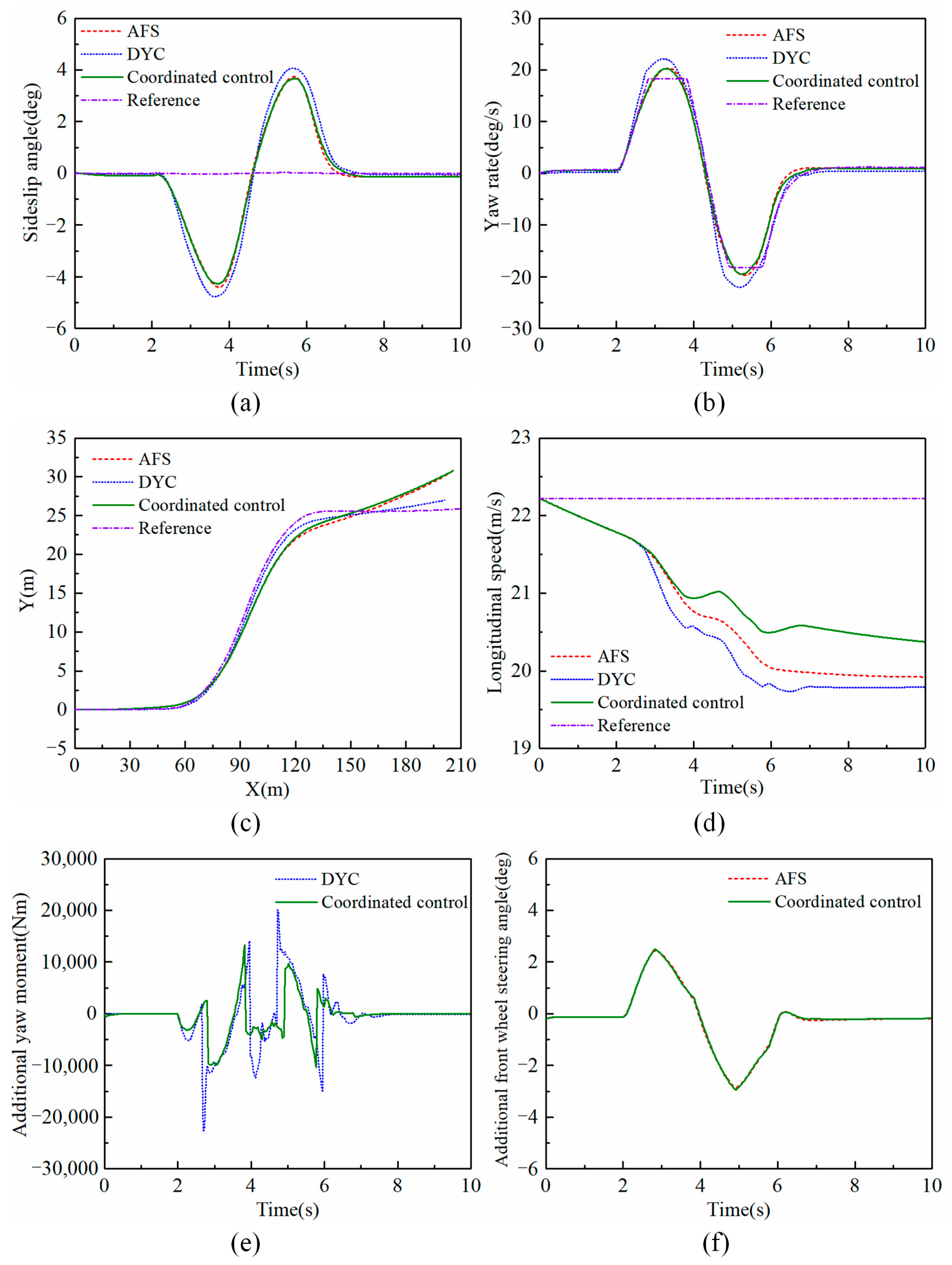
5.1. Maneuver 1: Single Lane Change under Peak Steering Angle 180°

The road adhesion coefficient is 0.85. The vehicle speed is 80 km/h. The maximum steering amplitude is 180°. The simulation results are illustrated in Figure 11a–f.
As can be seen from Figure 11a,b, the steering angle is relatively insignificant and the vehicle is in the stable region. For the sideslip angle and yaw rate, the control effects of the AFS system and the coordinated control system are not much different. Compared with the DYC system, they are closer to the ideal values. The control effect of the DYC system is slightly worse.
In terms of driving trajectory, as shown in Figure 11c, the vehicle controlled by DYC is closest to the ideal reference value. AFS is similar to the driving trajectory of coordinated control. As shown in Figure 11d, the longitudinal speed of the DYC system drops the fastest. The coordinated control drops the slowest, and its control effect is the best.
The additional yaw moment and additional front wheel steering angle are demonstrated in Figure 11e,f. Compared with the additional yaw moment of DYC control, the coordinated control has fewer sudden changes, and the values are smaller. It shows a better effect. The additional steering wheel angle of AFS and coordinated control are basically the same; hence they showed similar control effects.
The tracking errors of sideslip angle and yaw rate of the three strategies are respectively analyzed. The value of mean absolute error (MAE) and root mean square error (RMSE) is illustrated in Figure 12a,b. Whether the sideslip angle or the yaw rate, the value of the DYC method is the largest. The values of AFS and coordinated control are smaller, which also confirms that the AFS system mainly works in the stable region, and the AFS system plays the most important role at this time. Based on the results, the three control methods can effectively improve the stability of the vehicle.

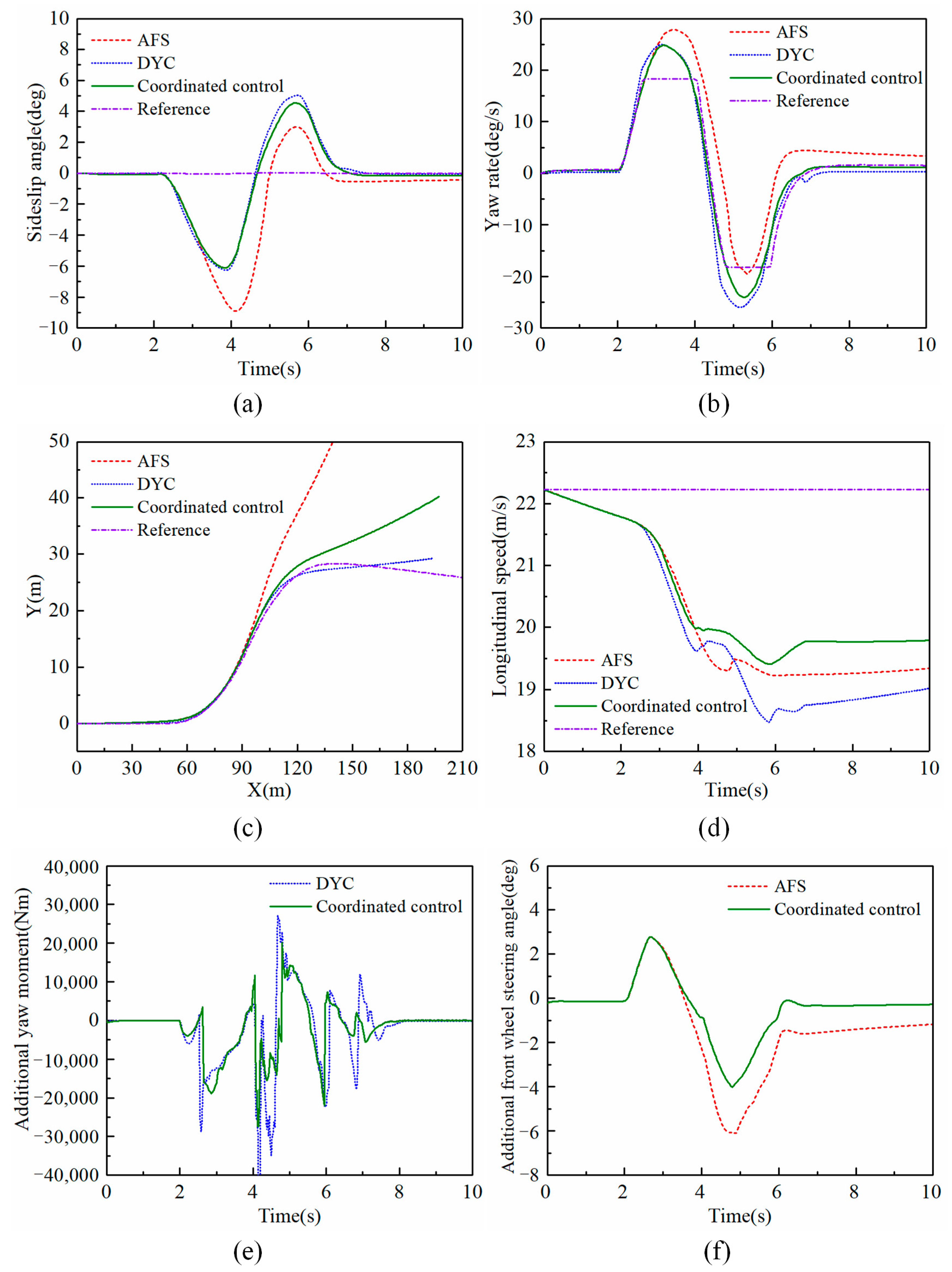
5.2. Maneuver 2: Single Lane Change under Peak Steering Angle 240°

The road adhesion coefficient is 0.85. The vehicle speed is 80 km/h. The maximum steering amplitude is 240°. The simulation results are illustrated in Figure 13a–f.
As displayed in Figure 13a,b, when the vehicle steering angle increases to 240°, the vehicle controlled by the single AFS system is almost destabilized and cannot work. DYC and coordinated control exhibit better control effect. The yaw rate and the sideslip angle are all stably controlled within a certain range. The vehicle did not lose its stability, reflecting the advantageous role of the DYC system in the unstable region. The yaw rate and the sideslip angle under the coordinated control are smaller than those under single DYC control and are the smallest among the three control systems.
In terms of the driving trajectory shown in Figure 13c, the vehicle controlled by DYC is closest to the ideal reference value. AFS loses its control effect and deviates from its ideal trajectory early. The effect of coordinated control is centered. The longitudinal speed of DYC decreases the fastest, as demonstrated in Figure 13d. The longitudinal speed of coordinated control is closer to the reference value, and the control effect is the best.
Although the additional yaw moment and additional front wheel steering angle required for coordinated control are smaller, as illustrated in Figure 13e,f, the control effect is better. This shows the superiority of the proposed coordinated control strategy.
The same conclusion can be confirmed by MAE and RMSE in Figure 14a,b. The values of coordinated control are smaller. It indicates that sideslip angle and yaw rate are closest to the ideal reference values. It combines the advantages of the AFS system and the DYC system well. Among the three methods, it has the best control effect. The AFS control effect is the worst, which also confirms that the AFS system will lose its effect when it works in unstable areas such as large steering angles.

6. Conclusions

This paper proposes a coordinated control strategy based on AFS and DYC methods to improve the stability and maneuverability of distributed drive electric bus. The strategy can not only improve performance under general working conditions but also in extreme cases, such as low road adhesion coefficient and low speed.
A vehicle state observer based on SMO and ANFIS was designed to improve observation accuracy with the objective of better studying the stability of the bus during steering. The simulation results demonstrate the effectiveness of the observer. The phase plane method is used to calculate the stability region for different driving conditions, which provides a reference for the coordinated control strategy executor. Through the weight function, the execution proportion of the AFS system and the DYC system is flexibly allocated. The simulation and verification in two cases of single-lane change steering condition are carried out. Through the analysis of MAE and RMSE of the sideslip angle and yaw rate compared to the ideal value, the effectiveness of the proposed coordinated control strategy is verified.
The results illustrate that the coordinated control strategy has excellent performances. The AFS system and the DYC system can be well-coordinated under different driving conditions, adapt to various extreme environments, and maintain the stability and maneuverability of the bus. However, due to the limited capability of the authors and some objective conditions, the state parameter estimation algorithm and yaw stability coordinated control strategy developed in this paper are mainly verified by offline simulation, and further hardware-in-the-loop and actual vehicle validation are subsequently required.

Author Contributions

Conceptualization, J.L. and T.Z.; methodology, T.Z.; software, T.Z.; validation, L.S. and F.Z.; formal analysis, J.L.; investigation, L.S. and F.Z.; resources, Y.Z., L.S. and F.Z.; data curation, J.L. and T.Z.; writing—original draft preparation, J.L. and T.Z.; writing—review and editing, T.Z.; visualization, T.Z.; supervision, J.L.; project administration, J.L.; funding acquisition, Y.Z. and J.L. All authors have read and agreed to the published version of the manuscript.

Funding

This work is supported by the National Key Research and Development Program of China (2021YFB2500704), National Natural Science Foundation of China (52075188), Open fund of Fujian Key Laboratory of Automotive Electronics and Electric Drive (KF-X19001).

Data Availability Statement

Not applicable.

Conflicts of Interest

The authors declare no conflict of interest.

References

  1. Wu, J.; Cheng, S.; Liu, B.; Liu, C. A Human-Machine-Cooperative-Driving Controller Based on AFS and DYC for Vehicle Dynamic Stability. Energies 2017, 10, 1737. [Google Scholar] [CrossRef] [Green Version]
  2. Lin, J.; Zou, T.; Zhang, F.; Zhang, Y. Yaw Stability Research of the Distributed Drive Electric Bus by Adaptive Fuzzy Sliding Mode Control. Energies 2022, 15, 1280. [Google Scholar] [CrossRef]
  3. Xu, H.; Zhao, Y.; Pi, W.; Wang, Q.; Lin, F.; Zhang, C. Integrated Control of Active Front Wheel Steering and Active Suspension Based on Differential Flatness and Nonlinear Disturbance Observer. IEEE Trans. Veh. Technol. 2022, 71, 4813–4824. [Google Scholar] [CrossRef]
  4. Tian, J.; Wang, Q.; Ding, J.; Wang, Y.; Ma, Z. Integrated Control with DYC and DSS for 4WID Electric Vehicles. IEEE Access 2019, 7, 124077–124086. [Google Scholar] [CrossRef]
  5. Chen, J.; Guo, C.; Hu, S.; Sun, J.; Langari, R.; Tang, C. Robust Estimation of Vehicle Motion States Utilizing an Extended Set-Membership Filter. Appl. Sci. 2020, 10, 1343. [Google Scholar] [CrossRef] [Green Version]
  6. Li, L.; Ran, X.; Wu, K.; Song, J.; Han, Z. A novel fuzzy logic correctional algorithm for traction control systems on uneven low-friction road conditions. Veh. Syst. Dyn. 2015, 53, 711–733. [Google Scholar] [CrossRef]
  7. Boada, B.L.; Boada, M.J.L.; Diaz, V. Vehicle sideslip angle measurement based on sensor data fusion using an integrated ANFIS and an Unscented Kalman Filter algorithm. Mech. Syst. Signal Process. 2016, 72–73, 832–845. [Google Scholar] [CrossRef] [Green Version]
  8. Zhang, F.; Wang, Y.; Hu, J.; Yin, G.; Chen, S.; Zhang, H.; Zhou, D. A Novel Comprehensive Scheme for Vehicle State Estimation Using Dual Extended H-Infinity Kalman Filter. Electronics 2021, 10, 1526. [Google Scholar] [CrossRef]
  9. Chen, T.; Chen, L.; Xu, X.; Cai, Y.; Jiang, H.; Sun, X. Estimation of Longitudinal Force and Sideslip Angle for Intelligent Four-Wheel Independent Drive Electric Vehicles by Observer Iteration and Information Fusion. Sensors 2018, 18, 1268. [Google Scholar] [CrossRef] [Green Version]
  10. Melzi, S.; Sabbioni, E. On the vehicle sideslip angle estimation through neural networks: Numerical and experimental results. Mech. Syst. Signal Process. 2011, 25, 2005–2019. [Google Scholar] [CrossRef]
  11. Hu, J.-S.; Wang, Y.; Fujimoto, H.; Hori, Y. Robust Yaw Stability Control for In-Wheel Motor Electric Vehicles. IEEE ASME Trans. Mechatron. 2017, 22, 1360–1370. [Google Scholar] [CrossRef]
  12. Song, Y.; Shu, H.; Chen, X.; Luo, S. Direct-yaw-moment control of four-wheel-drive electrical vehicle based on lateral tyre–road forces and sideslip angle observer. IET Intell. Transp. Syst. 2018, 13, 303–312. [Google Scholar] [CrossRef]
  13. Sun, P.; Trigell, A.S.; Drugge, L.; Jerrelind, J. Energy efficiency and stability of electric vehicles utilising direct yaw moment control. Veh. Syst. Dyn. 2020, 60, 930–950. [Google Scholar] [CrossRef]
  14. Lu, C.; Yuan, J.; Zha, G.; Ding, S. Sliding Mode Integrated Control for Vehicle Systems Based on AFS and DYC. Math. Probl. Eng. 2020, 2020, 1–8. [Google Scholar] [CrossRef]
  15. Ahmadian, N.; Khosravi, A.; Sarhadi, P. Driver assistant yaw stability control via integration of AFS and DYC. Veh. Syst. Dyn. 2021, 60, 1742–1762. [Google Scholar] [CrossRef]
  16. Jin, L.; Gao, L.; Jiang, Y.; Chen, M.; Zheng, Y.; Li, K. Research on the control and coordination of four-wheel independent driving/steering electric vehicle. Adv. Mech. Eng. 2017, 9, 1687814017698877. [Google Scholar] [CrossRef] [Green Version]
  17. Mousavinejad, E.; Han, Q.-L.; Yang, F.; Zhu, Y.; Vlacic, L. Integrated control of ground vehicles dynamics via advanced terminal sliding mode control. Veh. Syst. Dyn. 2016, 55, 268–294. [Google Scholar] [CrossRef]
  18. Ma, Y.; Chen, J.; Zhu, X.; Xu, Y. Lateral stability integrated with energy efficiency control for electric vehicles. Mech. Syst. Signal Process. 2019, 127, 1–15. [Google Scholar] [CrossRef]
  19. Mirzaeinejad, H.; Mirzaei, M.; Rafatnia, S. A novel technique for optimal integration of active steering and differential braking with estimation to improve vehicle directional stability. ISA Trans. 2018, 80, 513–527. [Google Scholar] [CrossRef]
  20. Ahmadian, N.; Khosravi, A.; Sarhadi, P. Adaptive yaw stability control by coordination of active steering and braking with an optimized lower-level controller. Int. J. Adapt. Control Signal Process. 2020, 34, 1242–1258. [Google Scholar] [CrossRef]
  21. Hu, X.; Chen, H.; Li, Z.; Wang, P. An Energy-Saving Torque Vectoring Control Strategy for Electric Vehicles Considering Handling Stability Under Extreme Conditions. IEEE Trans. Veh. Technol. 2020, 69, 10787–10796. [Google Scholar] [CrossRef]
  22. Zhao, H.; Lu, X.; Chen, H.; Liu, Q.; Gao, B. Coordinated Attitude Control of Longitudinal, Lateral and Vertical Tyre Forces for Electric Vehicles Based on Model Predictive Control. IEEE Trans. Veh. Technol. 2021, 71, 2550–2559. [Google Scholar] [CrossRef]
  23. Jing, C.; Shu, H.; Shu, R.; Song, Y. Integrated control of electric vehicles based on active front steering and model predictive control. Control Eng. Pract. 2022, 121, 105066. [Google Scholar] [CrossRef]
  24. Huang, W.; Wong, P.K. Integrated vehicle dynamics management for distributed-drive electric vehicles with active front steering using adaptive neural approaches against unknown nonlinearity. Int. J. Robust Nonlinear Control 2019, 29, 4888–4908. [Google Scholar] [CrossRef]
  25. Ahmadian, N.; Khosravi, A.; Sarhadi, P. Integrated model reference adaptive control to coordinate active front steering and direct yaw moment control. ISA Trans. 2020, 106, 85–96. [Google Scholar] [CrossRef]
  26. Termous, H.; Shraim, H.; Talj, R.; Francis, C.; Charara, A. Coordinated control strategies for active steering, differential braking and active suspension for vehicle stability, handling and safety improvement. Veh. Syst. Dyn. 2018, 57, 1494–1529. [Google Scholar] [CrossRef]
  27. Jin, X.; Yu, Z.; Yin, G.; Wang, J. Improving Vehicle Handling Stability Based on Combined AFS and DYC System via Robust Takagi-Sugeno Fuzzy Control. IEEE Trans. Intell. Transp. Syst. 2018, 19, 2696–2707. [Google Scholar] [CrossRef]
  28. Zhao, H.; Chen, W.; Zhao, J.; Zhang, Y.; Chen, H. Modular Integrated Longitudinal, Lateral, and Vertical Vehicle Stability Control for Distributed Electric Vehicles. IEEE Trans. Veh. Technol. 2019, 68, 1327–1338. [Google Scholar] [CrossRef]
  29. Liang, Y.; Li, Y.; Yu, Y.; Zheng, L. Integrated lateral control for 4WID/4WIS vehicle in high-speed condition considering the magnitude of steering. Veh. Syst. Dyn. 2019, 58, 1711–1735. [Google Scholar] [CrossRef]
  30. Ni, J.; Hu, J.; Xiang, C. Envelope Control for Four-Wheel Independently Actuated Autonomous Ground Vehicle Through AFS/DYC Integrated Control. IEEE Trans. Veh. Technol. 2017, 66, 9712–9726. [Google Scholar] [CrossRef]
  31. Han, Z.; Xu, N.; Chen, H.; Huang, Y.; Zhao, B. Energy-efficient control of electric vehicles based on linear quadratic regulator and phase plane analysis. Appl. Energy 2018, 213, 639–657. [Google Scholar] [CrossRef]
  32. Liu, W.; Xiong, L.; Leng, B.; Meng, H.; Zhang, R. Vehicle Stability Criterion Research Based on Phase Plane Method. In Proceedings of the WCX™ 17: SAE World Congress Experience, SAE Technical Paper Series, Detroit, MI, USA, 4–6 April 2017. [Google Scholar] [CrossRef]
  33. Chen, W.; Liang, X.; Wang, Q.; Zhao, L.; Wang, X. Extension coordinated control of four wheel independent drive electric vehicles by AFS and DYC. Control Eng. Pract. 2020, 101, 104504. [Google Scholar] [CrossRef]
Figure 1. 2-DOF vehicle model.
Machines 11 00640 g001
Figure 2. 7-DOF vehicle model.
Machines 11 00640 g002
Figure 3. Vehicle wheel force analysis schematic.
Machines 11 00640 g003
Figure 4. Structure of the state observer.
Machines 11 00640 g004
Figure 5. Structure of the ANFIS.
Machines 11 00640 g005
Figure 6. Estimated parameters at high adhesion coefficient and high speed. (a) Lateral speed, (b) Sideslip angle.
Machines 11 00640 g006
Figure 7. Estimated parameters at low adhesion coefficient and low speed. (a) Lateral speed, (b) sideslip angle.
Machines 11 00640 g007
Figure 8. Overall structure of the coordinated control strategy.
Machines 11 00640 g008
Figure 9. Stable domain division method diagram.
Machines 11 00640 g009
Figure 10. Stability index.
Machines 11 00640 g010
Figure 11. The parametric simulation results under maneuver 1. (a) Sideslip angle, (b) Yaw rate, (c) Driving trajectory, (d) Longitudinal speed, (e) Additional yaw moment, (f) Additional front wheel steering angle.
Machines 11 00640 g011
Figure 12. The MAE and RMSE of tracking errors under maneuver 1. (a) Sideslip angle, (b) Yaw rate.
Machines 11 00640 g012
Figure 13. The parametric simulation results under maneuver 2. (a) Sideslip angle, (b) Yaw rate, (c) Driving trajectory, (d) Longitudinal speed, (e) Additional yaw moment, (f) Additional front wheel steering angle.
Machines 11 00640 g013
Figure 14. The MAE and RMSE of tracking errors under maneuver 2. (a) Sideslip angle, (b) Yaw rate.
Machines 11 00640 g014
Table 1. Parameters of distributed drive electric bus.
ParametersSymbolValue
Vehicle massm7620 kg
Distance from CG to front axlea3105 mm
Distance from CG to rear axleb1385 mm
Wheelbased2030 mm
Yaw moment of inertiaIz30,782.4 kg·m2
Effective radius of wheelRe510 mm
Wheel moment of inertiaJw14 kg·m2
Height of CGhg1200 mm
Acceleration of gravityg9.8 m/s2
Table 2. Fuzzy control rules.
eψeβ
NBNSZOPSPB
NBZOPSPBPSZO
NSNSZOPBZONS
ZONBNBNBNBNB
PSNSZOPBZONS
PBZOPSPBPSZO
NB denotes negative big, NS denotes negative small, ZO denotes zero, PS denotes positive small, and PB denotes positive big.
Disclaimer/Publisher’s Note: The statements, opinions and data contained in all publications are solely those of the individual author(s) and contributor(s) and not of MDPI and/or the editor(s). MDPI and/or the editor(s) disclaim responsibility for any injury to people or property resulting from any ideas, methods, instructions or products referred to in the content.

