Vibration Resonance Spectrometry (VRS) for the Advanced Streaming Detection of Rotor Unbalance

Abstract

Determination of the diagnosis thresholds is crucial for the fault diagnosis of industry assets. Rotor machines under different working conditions are especially challenging because of the dynamic torque and speed. In this paper, an advanced machine learning based signal-processing innovation termed the multivariate state estimation technique is proposed to improve the accuracy of the diagnosis thresholds. A novel preprocessing technique called vibration resonance spectrometry is also applied to achieve a low computation cost capability for real-time condition monitoring. The monitoring system that utilizes the above methods is then applied for prognostics of a fan model as an example. Different levels of radial unbalance were added on the fan and tested, and then compared with the health state. The results show that the proposed methodology can detect the unbalance with a good accuracy and low computation cost. The proposed methodology can be applied for complex engineering assets for better predictive monitoring that could be processed with on-premise edge devices, or eventually a cloud platform due to its capacity for loss-less dimension reduction.

1. Introduction

Historically, accelerometers (vibration sensors) have been used for decades to detect problems in assets in many types of industrial problems that result in higher vibration levels, which can be precursors to failure [1,2,3,4,5,6]. Perhaps the greatest challenge for conventional vibrational surveillance of assets is the inherent “seesaw” effect between the sensitivity for catching incipient degradation mechanisms and their false alarms. This is a consequence of placing thresholds limits on the power spectral density (PSD) peak amplitude [7,8,9,10]. Monitoring system designers usually lower the thresholds to obtain a higher sensitivity for earlier warnings of the developing degradation mode. However, with variable performance assets, and especially with variability in ambient vibration levels, lowering these thresholds results in spurious alarms that have no significance at all. In most industries, false alarms from spurious trips of these thresholds are extremely costly, as the false alarms result in taking assets out of service unnecessarily. As a result, designers raise the alarm thresholds on peak responses. Consequently, if there is a new degradation mode, the degradation is usually severely underway, or the machine is dead before any alarm can be issued [11,12].

Current research on the rotor unbalance for the contact and non-contact measurement methods are as follows, Ewert et al. studied the difference between classical spectrum analysis and the higher-order bispectrum method for the permanent magnet synchronous motor [13]. Gangsar et al. used the support vector machine method to detect rotor unbalance [14]. Rahman et al. proposed an unbalance detection method based on online condition monitoring using the discrete wavelet transform [15]. Puerto et al. proposed a novel methodology for non-intrusive mechanical unbalance monitoring [16]. Furthermore, there have also been the development of several vibration signal analysis methods using non-contact measurements [17,18,19]. However, all the aforementioned methods lack the investigation of the thresholds for the detection of rotor unbalance.

Thresholds on vibration amplitudes are most appropriate for machines that have a constant load and run at a fixed speed for the life of the system, and for constant-load machines that happen to be in an environment with a stationary ambient vibration level (i.e., containing no other vibrating components that could provide a variable ambient vibration level). However, fixed workload components that run at fixed RPMs for life and are not mechanically coupled to any other components that add to the ambient vibration background are exceedingly rare. For rotating machinery with dynamic workloads, variable-speed performances, and mounting into structures containing other dynamically varying vibration sources, thresholds on gross vibrational amplitudes are very inefficient for detecting the early onset of degradation. These inefficiencies are a consequence of the threshold boundaries. Threshold alarm boundaries need to be set higher than the highest peak for the component at its highest load and the highest RPM setting when the ambient vibration levels are at their highest. This significantly lowers the “early warning” potential for prognostics, as thresholds on vibration amplitudes can be very inefficient when the components are not operating at peak load/performance conditions.

One solution to the threshold inefficiencies is to introduce a machine learning (ML) model for monitoring the vibration signals. A simple univariate model could be used, but multivariate models are significantly more accurate. However, vibration signals are generally univariate. A secondary hindrance is that vibration measurements are inherently of a high frequency, with sample rates for the vibrations being in the kHz range. The glut of data generated by these sensors quickly becomes unmanageable for storage, which makes vibration-based monitoring untenable [12,20,21,22]. Thus, vibration resonance spectrometry (VRS) has been proposed to process the data for the loss-less dimension reduction of the signals and produce a multivariate dataset from one vibration sensor that can be consumed by a ML model.

The VRS transforms a single univariate vibration or acoustic signal into 20 correlated time series signals that are predictive of an asset’s unique operational frequency signature. First, during the measurement phase, a deterministic periodic loading pattern, which covers the entire range of the asset operation, is introduced to excite the appropriate system dynamics in the frequency domain. The second stage is a preprocessing algorithm which is composed of several substages whereby vibration/acoustic measurements are manipulated with a frequency-domain to time-domain to frequency-domain double transformation. The double transformation ostensibly reduces the dimension of the data without causing a loss in prognostic information. In the final stage, the output from VRS is inputted into a ML algorithm, thereby generating a model for the subsequent monitoring of new measurements. ML monitoring informs condition-based decisions regarding the state of the mechanical, electromechanical, or thermal-hydraulic system. The ML algorithm is integrated into the multivariate state estimation technique (MSET), which is defined as a nonlinear regression-based technique. It is best suited for anomaly detection in time series data. It has been widely adopted in many business-critical industries for over 20 years. It has been redeveloped in recent years to make it scalable to large collections of telemetry sensors for big prognostic use cases. There are several reasons for such a widespread adoption. First, the MSET has significant advantages regarding their great accuracy and low false alarm and missed alarm rates. They are crucial especially in the field of anomaly detection, with false alarms leading to unnecessary asset shutdowns and missed alarms leading to catastrophic failures, both of which are very costly. Furthermore, the overhead compute cost of the MSET is much lower compared to the other prognostic algorithms such as neural networks and support vector machines due to its deterministic mathematical model, and this is important for streaming prognostics which involves tens of thousands of sensors [10,20,23,24,25,26].

In this paper, a multivariate state estimation technique and vibration resonance spectrometry have been proposed to improve the accuracy of diagnosis thresholds. Firstly, the specifics of the VRS methodology along with several design choices and algorithmic structures are presented. Then, the process with the ML monitoring of telemetry with MSET are discussed. Next, the experimental setup and the parameter settings of the unbalanced fans are introduced, and different levels of radial unbalance were added on the fan and assessed. Finally, the results show that the proposed methodology can detect the unbalance with a good accuracy and low computation cost.

2. Detection Methodology

2.1. Principals of the Method

When VRS is combined with other auxiliary-supporting computational agents, it is capable of robust prognostics for all types of mechanical, electromechanical, and thermal-hydraulic flow systems. The algorithm autonomously discriminates the multi-bin operation frequency signatures for the predictive-based health monitoring of an asset. Predicated on solving two major hindrances to vibration predictive monitoring, being the high-frequency sample rates, and low sensitivity to subtle degradation, the algorithm solves these inadequacies in a multi-stage analytical framework.

First, during the measurement phase, a deterministic oscillatory loading pattern that covers the entire range of the asset operation is introduced to excite the appropriate system dynamics in the frequency domain. The second stage is a preprocessing algorithm and is the cornerstone of VRS. The second stage is composed of several substages whereby the accelerometer measurements are manipulated with a frequency-domain to time-domain to frequency-domain double transformation. The double transformation ostensibly reduces the dimension of the data without causing a loss in prognostic information. In the final stage, the time series from VRS are inputted into a ML algorithm, leading to the generation of a model for the subsequent monitoring of new measurements. ML monitoring informs predictive-based decisions regarding the state of the mechanical, electromechanical, or thermal-hydraulic systems.

2.2. Vibration Measurement Training Regimen

Utilizing ML to monitor an asset requires the training data to encompass the entire range of the system operation. For example, if the training data for monitoring a car only contains city driving measurements, the model will generate alarms if the car were to begin highway driving. Additionally, it is common for mechanical assets to operate in a small subset of the spectrum of operation for long periods. To continue with the car as an example, if it operates mostly in the city, its driving will be on the streets, oscillating between idle and approximately 40 miles per hour, with either short spurts of regular freeway driving or long-range driving on the freeway, but infrequently. In the first scenario, it will take a long time to log enough freeway training data to generate reliable predictions. In the second scenario, one long trip may provide enough freeway measurements for a valid training set, but with much less opportunities to do so. Furthermore, most drivers never reach a peak or maximum performance in a car regardless how long and how often the car has been driven. Therefore, it is necessary to incite the entire operational range during the initial stage of measurements to guarantee sufficient training data to generate a reliable model.

Another concern that is specific to vibration measurements is the magnitude of the stochastic noise measurement. Tracking vibration modes requires a high resolution and dense sampling to capture the true dynamics of the system, which are otherwise opaque, allowing for more opportunities for obtaining noisy measurements. Noise can also stem from how the vibration of a system is being measured, as vibrations are usually tracked globally and not through individual components in the system. Tracking global measurements as opposed to individual components of the system are generally more pragmatic, since storing and processing data from the individual components in a system are prohibitively expensive, or access to all the components may not be feasible. Moreover, global measurements track multiple components in parallel, and the emergent behavior of the system is more indicative of reality. Unfortunately, tracking system behavior generates noisy measurements as it is composed of multiple components that vibrate and resonate with their own unique frequencies.

To mitigate noise and guarantee adequate training data, the monitored asset runs through a short deterministic periodic loading pattern for a nominal amount of time. The workload must cycle through all known and valid operational states of the system. The pattern can be sophisticated if the asset has a programmable workload capability or can be extremely simple as toggling on/off, or idle/max several times in a “training” window. The technique is also indifferent to the shape of the periodic workload wave. The pattern can be sinusoidal in nature, saw tooth, or a square wave if the pattern is repeated. This training measurement regime ensures full operational classification and aids in processing downstream. The periodic pattern makes the asset operational signature more easily identifiable in the frequency domain, thereby bypassing noise that may have been overshadowing the representative frequencies of the system. The additional benefits to the determinism in the workload will be discussed in later sections.

2.3. VRS Preprocessing

The approach for the vibration analysis introduced in this study is composed of a frequency-domain to time-domain to frequency-domain double transformation, resulting in an optimal set of a finite number of narrow-band frequency bins. This creates a set of time series signals. The bins are sampled at a rate which matches the other sensor telemetry for the assets under surveillance, e.g., once every 2 or 5 s. Ideally, the fastest sampling rate for the other telemetry metrics (e.g., temperatures, voltages, currents, RPMs, etc.) is selected to sample the narrow-band frequency bin time series, thereby instituting real-time vibration monitoring. The bins are then averaged and ranked, resulting in a set of time series which are subsequently consumed by a machine learning algorithm, along with additional telemetry, to monitor the condition of rotating machinery and other mechanical systems.

2.3.1. Frequency Transformation

Once the raw measurements are recorded, there is an initial transformation into the frequency domain using a fast Fourier transform (FFT) and the PSD is calculated. The window or sample size for the FFT is determined by the fastest sample rate of the remaining telemetry monitoring in any given mechanical system, and this is the first stage in dimension reduction. The results are a set of time series that records the change in frequency across the entire frequency spectrum, up to the Nyquist frequency. While there are some distinctly excited frequencies that are representative of the operating frequency of the system, they lie in narrow bands of the entire sample spectrum. To isolate the operational signature narrow bands of frequencies are either grouped, or “binned,” and undergo a process for reducing noise within each group and ranking.

2.3.2. Frequency Binning

When a wide frequency spectrum is sampled, there will be unexcited frequencies that are essentially noise. To identify the more representative frequencies we split the frequency spectrum into several frequency bins. Subsequently, a technique to generate a time series signal that is a highly correlated average of the frequencies in the bin is applied. This not only reduces the problem size, but also gets rid of the noisy behavior in general. The process narrows the broad frequency spectrum and isolates the germane frequencies by “binning” the frequencies across the linearly spaced ranges, and then finds the most representative time series in the narrow band frequency bins by averaging the most highly correlated signals in the bin.

The first step is to decide the number of frequency bins to use for subdividing the spectrum. The total number of bins should be small enough to reduce the size of the spectrum data. In addition, the number of frequencies in each bin needs to be large enough to have a statistically significant sample guaranteeing the average time series comprises more than one frequency. The number of total bins in this study has been empirically determined to be 100 through previous work [27]. The value can either be reduced or increased depending on the context, but 100 has been found to be at the optimal intersection between the dimension reduction and the robust frequency characterization of an asset.

The number of frequencies in each bin will also influence these results. If each bin is of equal length, it is likely that a portion of the spectrum that is either minimally active or superfluous will be weighted too highly downstream. To account for the inequity in the measured spectrum, a weighting system is applied based on the root mean square (RMS) to determine the overall energy in each portion of the spectrum:

$$\begin{array}{c}RMS=\sqrt{\frac{A_0^2}{2}+{{\displaystyle \sum }}_{i=1}^{k-1}{A}_i^2+\frac{A_k^2}{2}}\end{array}$$

(1)

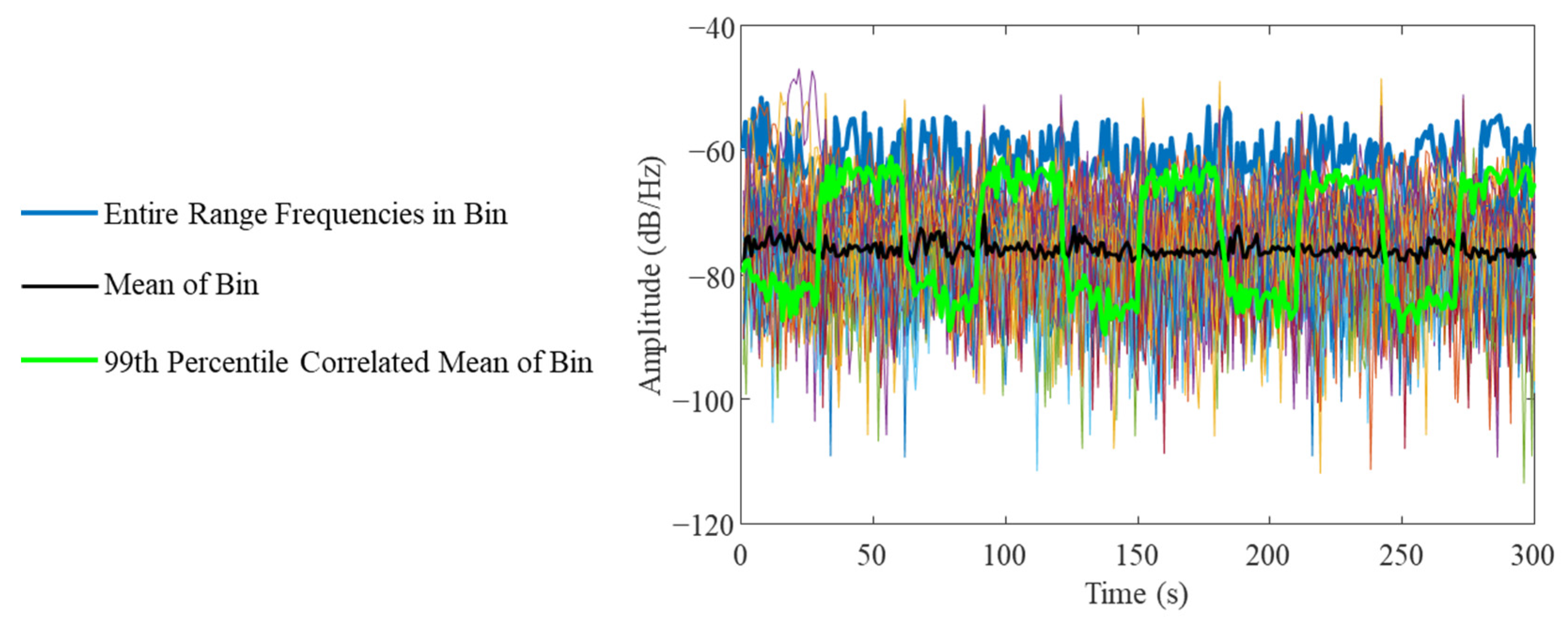
where $A$ is the discrete fast Fourier transform (DFFT) of the vibration signal. The segments of the spectrum with more energy have smaller bin sizes which proportionally increases the number of bins in that range. After grouping many of the bins are just random noise, while the most correlated prominently respond to the deterministic load sources. For some bins, a simple average over the frequencies in the bin will filter out the random noise yielding a signal with a greater signal-to-noise ratio as the random noise signals negate each other. To illustrate the motivations behind the correlation ranking average, an example of 100 frequency bins is displayed in Figure 1. Unfortunately, most bins are a mixture of noisy measurements, which are unresponsive to the load activity, and the simple average can result in a signal with less range (black). Instead, a subset of signals inside the frequency bin with the best inter-correlations are averaged, further filtering out the noise, yielding a high noise ratio signal (green), and revealing the dynamic pattern of the workload.

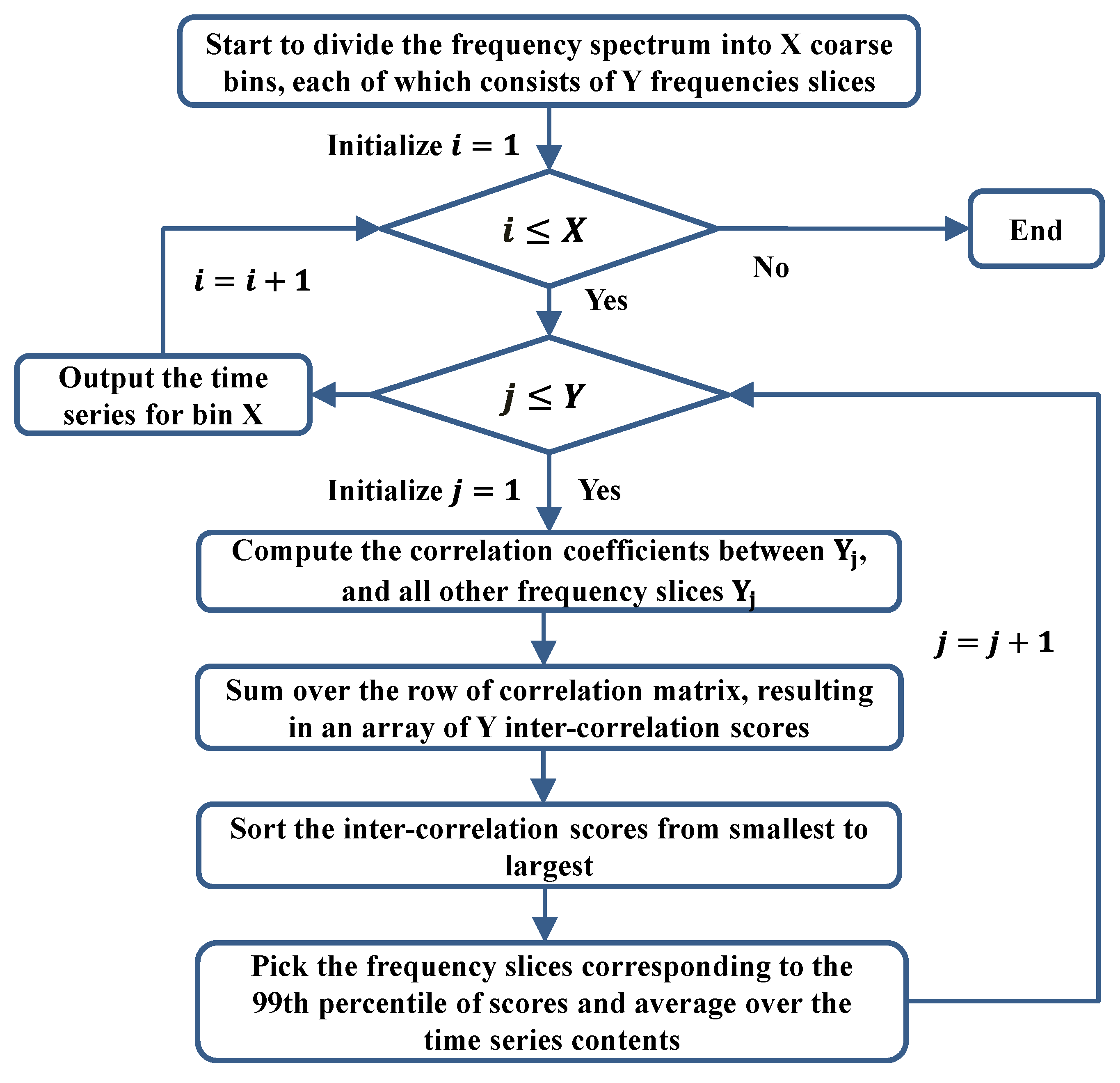
The algorithm structure is presented in Figure 2 to facilitate the explication of the process. All the signals in the bin go through a correlation matrix assessment, and the correlation coefficients are summed over the signals and sorted from the lowest to the highest. Then, the signals corresponding to the top one percentile are selected and averaged, yielding a single time series signal for that frequency bin. The percentile is utilized as the threshold instead of the correlation coefficient; therefore, this approach is adaptive and can be applied to any size frequency bin with any SNR distributions.

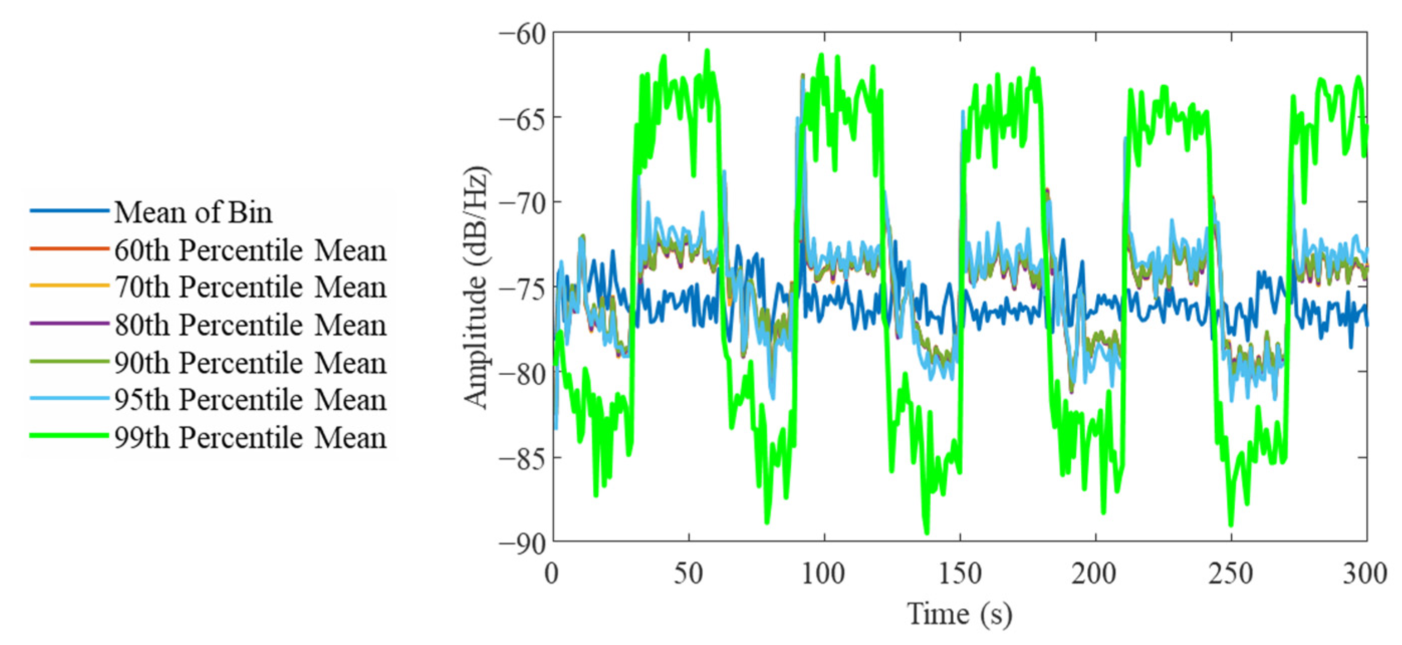
The 99th percentile was chosen as the “threshold” to sort out the best frequencies as it captures the signal dynamic range, but also retains more than one frequency signal per bin. Figure 3 shows a sensitivity test with different percentile thresholds and their resulting averages. It was found that between the 90th and 99th percentiles, there was a significant improvement in terms of a greater dynamic range and clearer shape of the periodic workload, but this was found to not increase the likelihood of the too few available frequencies guaranteed by the lower thresholds.

2.3.3. Frequency Identification

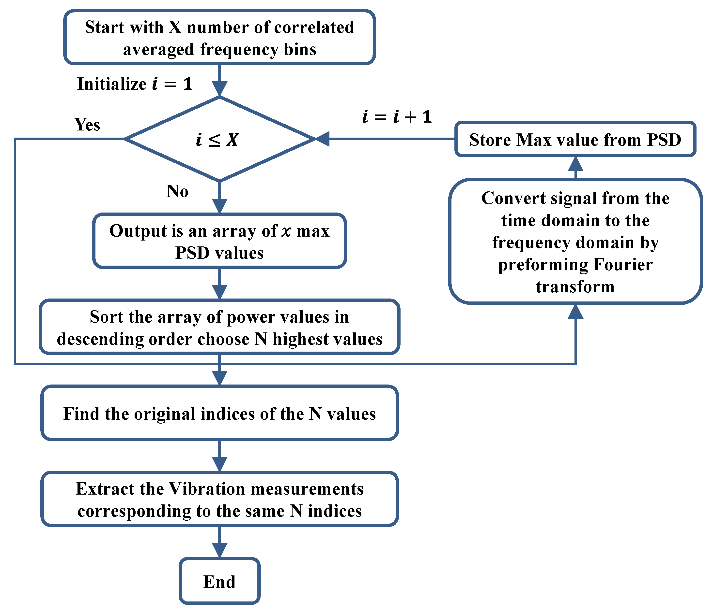
After the binning step, a sorting process is conducted to further reduce the problem size by discarding the frequency bins that are least representative of the operational frequencies of the system. The signals with the strongest frequency components in the spectrogram are chosen while the remainder are ignored. This step is greatly enhanced by the deterministic loading pattern. To determine the strongest frequency components, the resultant 100 time series from the binning step are transformed into the frequency domain again. The bins are sorted by the magnitude of the PSD. After the sorting, the number of bins that are discarded is dependent on the sensitivity requirements of the system. In this study, the top 20% of the discrete frequency bins were recommended for selection based on the height of the peak in the frequency domain. This was empirically determined to be the most representative of the frequency behavior of most assets. The algorithm by which the bins are sorted is presented in Figure 4 below.

Without the deterministic workload, the ranking process becomes much more ambiguous due to several factors that can influence the ranking. For example, a trend can be introduced into the time domain caused by an exogenous or stochastic process that does not directly influence the system. If this occurs, the affected bin, when converted into the frequency domain with a limited sample, will have a large PSD peak near 0 Hz. The reason for the large peaks is that the low frequency will generate a large Fourier coefficient. The magnitude of the low frequency can overshadow the remaining PSD peaks resulting in a high-ranking bin that is not representative of the operational signature of the system. Another source of ambiguity is the variation in excited frequencies which can be dependent on the operational state during the instance of measurements. This variation can also result in formation of outlier frequencies with a large PSD peak, resulting in an inconsistent sorting.

When the deterministic periodic workload is introduced into the training measurements, the precision of the sorting increases by utilizing the known frequency for ranking. For example, if the workload is programed with a cycle period of 1 min, the frequencies that are most relevant to the operational signature of the system will be excited by the workload, thereby generating a dominant peak at 1 min in the frequency domain and all other peaks can be ignored during sorting. The loading pattern also introduces consistency into the measurements and the operation of the system, which thereby reduces noise as a result. Finally, as aforementioned, the periodic workload should cover the entire range of normal operation. All these properties lead to the consistent frequency identification for a system unless the condition of the system has degraded.

3. MSET ML-Based Monitoring

The MSET has two primary phases: training and inferencing. The model is trained with the operating-frequency-data from a system. Here the system does not have to be a brand new asset, but an asset that is certified to have no degradation, and the MSET estimates are subsequently produced with this model. After that, the pairwise residuals between the MSET estimates and the actual values are computed and sent to an anomaly detection module called the sequential probability ratio test (SPRT) [24,25,26]. The SPRT performs two statistical hypothesis tests, whereby the mean and variance shift between the reference distribution and the degraded distribution are quantified to identify the anomalies. The SPRT allows the users to specify both the false alarm rate and missed alarm rate, which thereby avoids the conventional trade-offs between the low false alarm rate and low missed alarm rate.

3.1. Training

The training for the MSET is composed of measurements taken from a healthy system. These measurements consist of highly correlated features from a mechanical system, such as RPMs, voltages, and currents. In this study, the training consists of 20 frequencies that were identified during a period of healthy operation. In the field, these 20 frequencies would be included with the remaining telemetry in the model for more accurate and precise condition monitoring. However, for laboratory experiments, ML would be trained solely on the healthy operational signature.

3.2. Monitoring

During the monitoring phase, the measurements will be continued after the system has been altered. The alteration in this case would be several radial imbalances that gradually increase in severity. The frequency bins that are monitored for the imbalanced measurements are identical to the 20 bins determined during the binning and sorting phase while the system is healthy. The motivation for doing so is that a shift in the operational frequency often occurs when there is a damage in the system. For example, if a gear tooth in a gearbox chips, the motor power and the RPM will likely increase to compensate for the damage, resulting in higher frequency vibrations [28]. The frequency behavior of the healthy state will be the most indicative of normality.

4. Experimental Setup

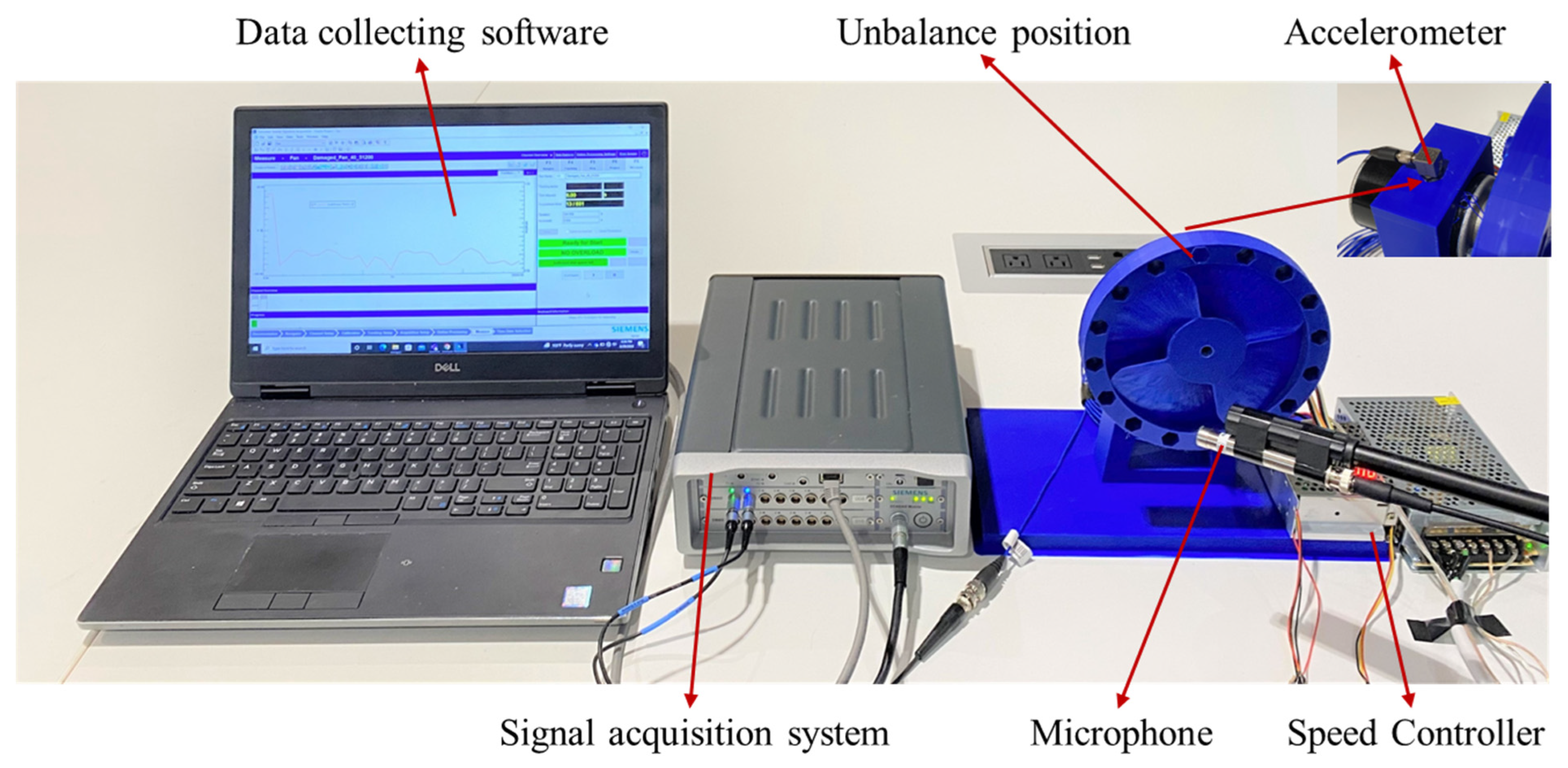
The experimental testing was performed on a 3D-printed fan that is a proxy for a mechanical impellor blade in a motor or rotary machinery. There were two unique impellor states: healthy and damaged. The healthy state of the impellor was a fan that was uniformly balanced. A few holes were designed to be in the circumferential direction. A small mass can be inserted into the hole thereby introducing an imbalance to the fan. To obtain the measurements, a tri-axial accelerometer (PCB TLD333B30) and a microphone (PCB 378B02) were utilized, which have a good sensitivity deviation in complex measurement environments. The calibration sensitivity of the accelerometers was 103.3 mV/g. We also used the sound level calibrator (B&K 4231) to calibrate the microphone sensor. The accelerometer was placed onto the impellor mount. and the microphone was placed in front of the impellor. The entire experimental setup was placed in a whisper room to avoid environmental noise that could influence the microphone measurements. The vibration and acoustic time series signals were recorded, and the experiment was repeated 4 separate times for each state.

The entire unbalanced fan assembly is depicted in Figure 5. During the measurement, the fan speed was a periodical workload, which ramped up and down from 20% to 50% of the nominal speed (3000 rpm), respectively. The tri-accelerometer was placed on top of the fan bracket and the microphone was placed in the upper front of the fan at an angle to avoid air turbulence. The Simcenter SCADAS mobile and recorder were used to measure the vibration data using the ICP mode. Four rings of different weights were used to create fan unbalance at different levels. The measurement process was repeated 4 times at a sampling frequency of 16.384 kHz, each lasting 600 s. The measured data included the acoustics and vibration signals in three directions. We used the data in the radial direction of the fan model by analyzing the performance of the 4 sets of data.

5. Results and Discussions

As mentioned before, the current techniques in vibration monitoring relies on tracking the amplitude of the peaks in the frequency domain. However, there are many pitfalls to these methods. First, it is often difficult to determine which peaks are important and in which ranges as the data can be noisy. Additionally, monitoring one or a few peaks limits the focus on one or two dominant peaks and thus narrows the focus of inspection. These issues can lead to expensive false alarms, and in some cases results in deleterious missed alarms. Second, these methods generate massive amounts of vibration measurements, which require averaging or dimension reduction techniques, and thereby renders real-time monitoring impossible. Lastly, the monitoring systems are generally complicated and require an expensive subject matter expert (SME) to initiate, maintain, and monitor the systems as part of the custom on-premise solutions. The VRS and MSET techniques allow the user to automate vibration analysis with a better sensitivity to degradation and without the need for a SME. In this section, the data generated from the fan and analysis using current VRS and MSET techniques will be discussed.

5.1. Measurements

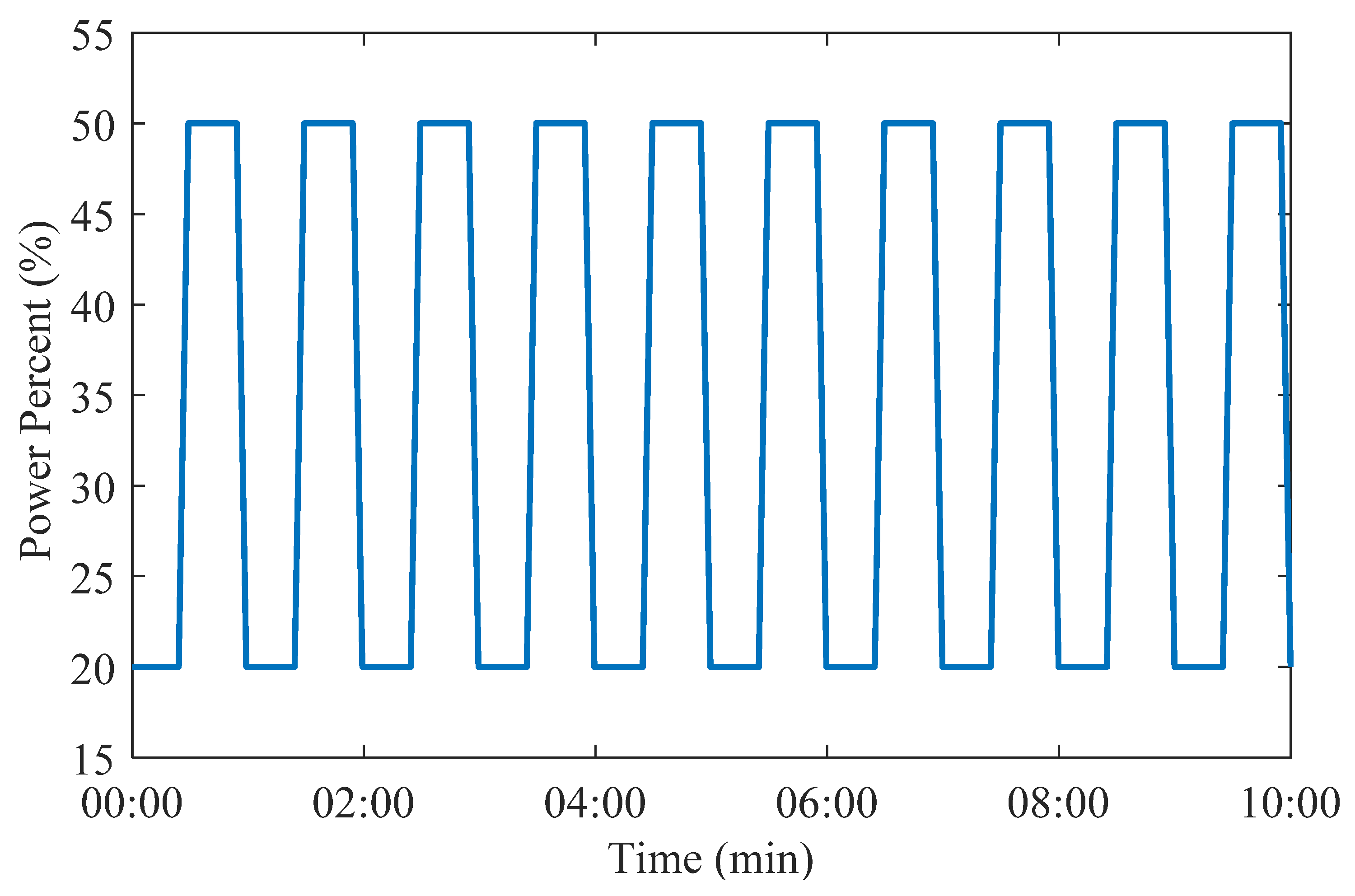
To identify the frequency bins that are unique to the system more easily, a periodic workload was introduced into the measurements. Due to experimental constraints, the fan speed could not be programmatically controlled, and a square-wave oscillation was implemented for simplicity. The pattern is illustrated in Figure 6, where one period of the square wave is equal to one minute. The wave measurements were initiated when the fan motor was at 20% power capacity for the first 30 s, then increased to 50% for the next 30 s, and subsequently dropped back down to 20%. This pattern was repeated for 10 min for both the healthy state and the unbalanced state. The 50% power threshold was determined to be the maximum operational capacity as it was found the chassis would crack when the power is greater than 50%.

5.2. Condition Monitoring Techniques

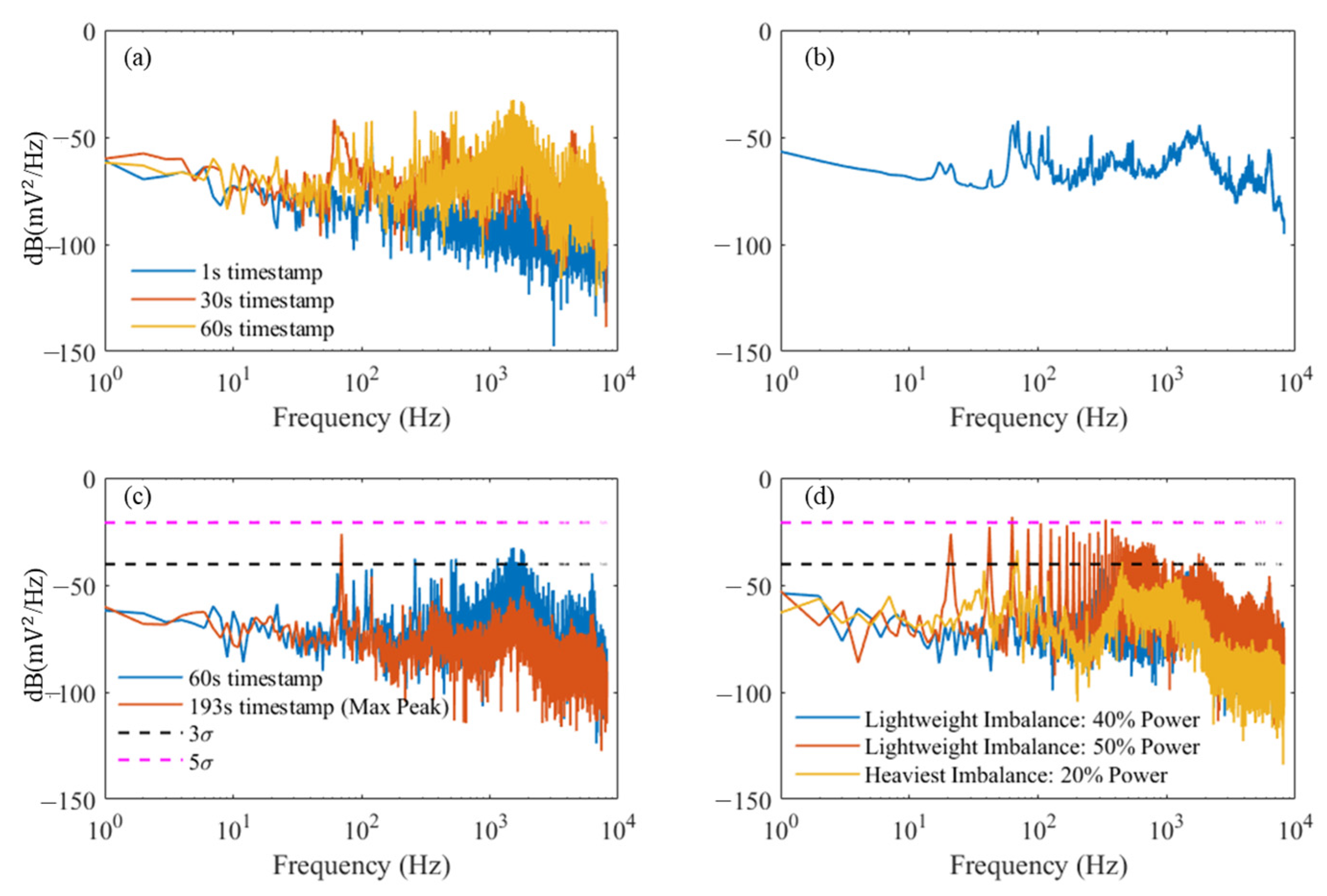
As a comparison, an analysis of the fan data utilizing current frequency domain monitoring practices was conducted [8,10,11,12]. Many of these methods are similar in nature whereby vibration measurements are converted into the frequency domain and the peaks with the largest magnitude are monitored over time. In Figure 7, the PSD of the measurements taken over 10 min was calculated, and the operational frequency was found to change over the course of the measurements. As such, the dominant frequencies changed over time.

Beginning with the first set, in Figure 7a, the PSD of the vibration measurements from the fan in the healthy state was calculated where no imbalance was present. From this, it was clear that the dominant peak was not uniform over time. One common technique is to sample the data over many periods and average the results [29]. This method is often used to determine the most prominent frequencies across the entire measurement set. Additionally, this process diminishes the noise thereby making the pertinent frequencies more identifiable. Figure 7b shows the resulting average PSD for the entire span of the healthy state measurements by which the thresholds were set. A standard statistical threshold is defined as three standard deviations (3σ) from the maximum peaks of the healthy measurements. Figure 7c shows the thresholds determined from Figure 7b, which were applied for monitoring a secondary set of healthy sate measurements. The red curve is the maximum peak occurrence in the healthy state measurements whereas the blue curve is another instance where the fan is operating at its maximum capacity. Both instances were deemed to trigger an alarm if the threshold of 3σ was employed. Therefore, in this instance, a threshold of 5σ was utilized to minimize the false alarms. Figure 7d shows the measurements for when the lightest weight imbalance was introduced. While the 5σ threshold does indicate that the fan has an imbalance, the alarm was only triggered when the fan is operating at its maximum capacity. This can be problematic, as if the operational capacity never reaches its maximum, the fault will be completely overlooked as a result.

Figure 7. The PSD spectrums with frequency thresholds: (a) comparison of healthy state measurements for different timestamps; (b) the entire spectrum; (c) comparison of thresholds and different timestamps for healthy state measurements; and (d) the thresholds comparison with the PSDs of different damaged states.

Figure 7. The PSD spectrums with frequency thresholds: (a) comparison of healthy state measurements for different timestamps; (b) the entire spectrum; (c) comparison of thresholds and different timestamps for healthy state measurements; and (d) the thresholds comparison with the PSDs of different damaged states.

The above analysis illustrates that these methods based on simple thresholding lack sensitivity to many defects. What is even more problematic is that these frequency signatures are unique to each asset and often to the type of fault. These issues can lead to expensive false alarms and in some cases deleterious missed alarms. There are other methods such as comparing the displacements or the velocity RMS, but again these metrics are also unique to the context [30]. In summary, these methods are only helpful for the non-destructive condition monitoring and binary assessment of whether the asset requires repair or not. There is no indication of the degradation severity, remaining useful life, how long the system has been faulty, and whether the outcome is state dependent.

5.3. The VRS Process and Predictive Monitoring

5.3.1. Frequency Analysis

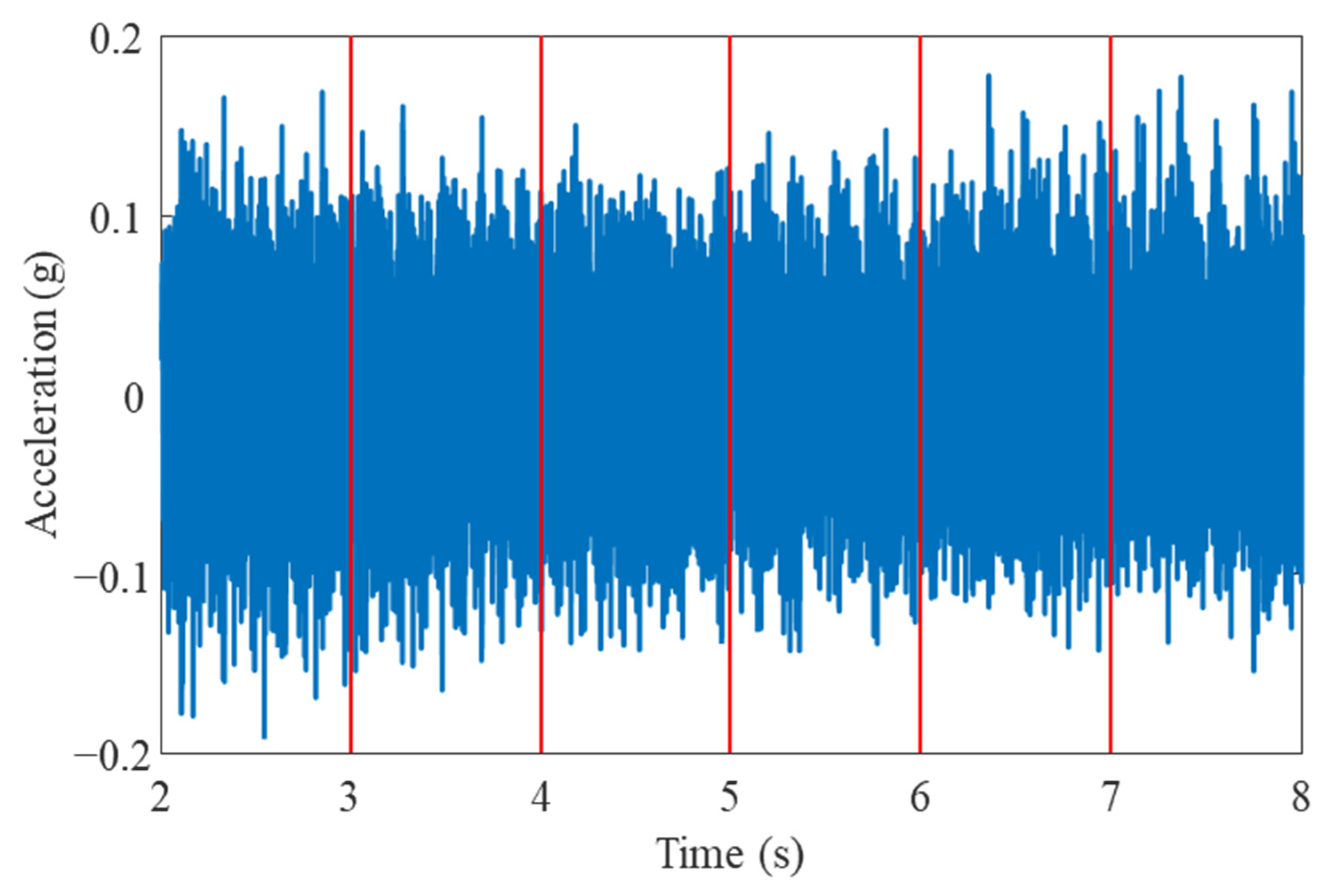
The first step in the VRS process is to convert the vibration measurements into the frequency domain. To initiate the analysis, the raw vibration signal was windowed to the intended sample rate as shown in Figure 8. For simplicity, the sample window chosen for this experiment was one second, as indicated by the vertical red line. The measurements lasted for 600 s but only 8 s were shown to make the window size more visually legible.

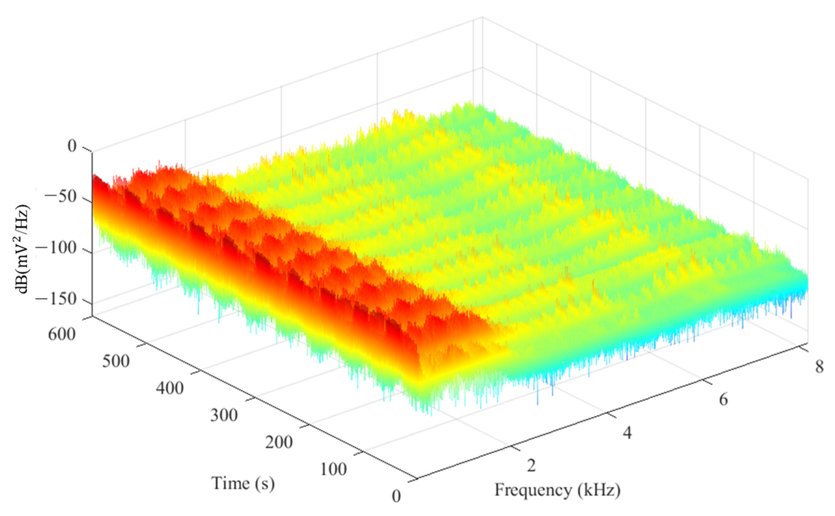
Each window was then transformed into the frequency domain through a FFT. Subsequently, the PSD was calculated resulting in a granular set of a time series which tracked the frequency change across the entire sample spectrum for each state of the fan. A moving Hann window was then applied to minimize edge artifacts in the frequency domain. An example for the balanced fan is presented in Figure 9. The dynamics of the oscillatory workload were visually apparent, and activity was skewed towards the first 3 kHz. The binning was weighted accordingly so that the more active part of the spectrums were prioritized. A more formal discussion of the weighting was continued in the next section.

5.3.2. Binning and Ranking

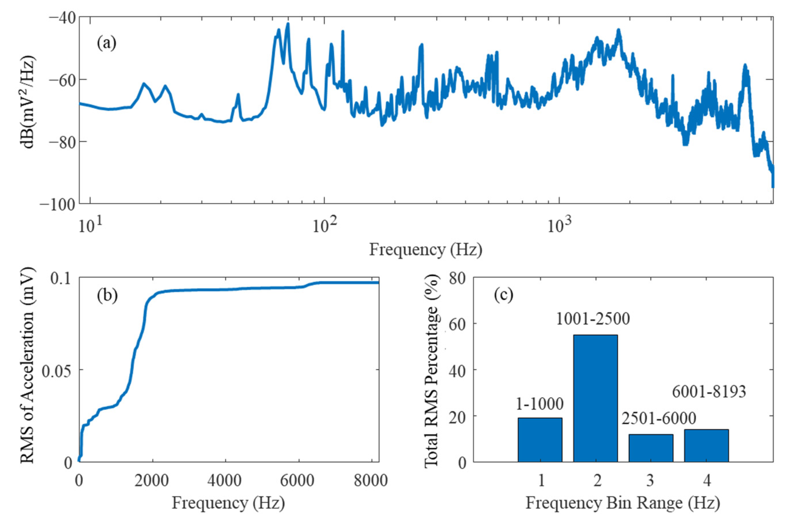
To determine the size of each frequency bin and therefore the weighting of each segment of the spectrum, the RMS metric in Equation (1) was applied to ascertain the energy content in each part of the spectrum. The first step was to ascertain the representative frequency spectrum for the entire set of healthy measurements by transforming the entire set of the healthy state vibration measurements with a PSD, as shown in Figure 10a. Then, the cumulative RMS across the entire frequency spectrum was calculated, as shown in Figure 10b, to assess the change in slope, which corresponds to an increase in the energy content of the spectrum. The frequency bin weighting was then determined by the percentage of the RMS that each portion of the spectrum contains, as shown in Figure 10c. In this case, the percentage of the RMS within the first 1000 Hz was approximately 18% which translates to 18 bins out of the 100 total bins being dedicated to the initial 1kHz.

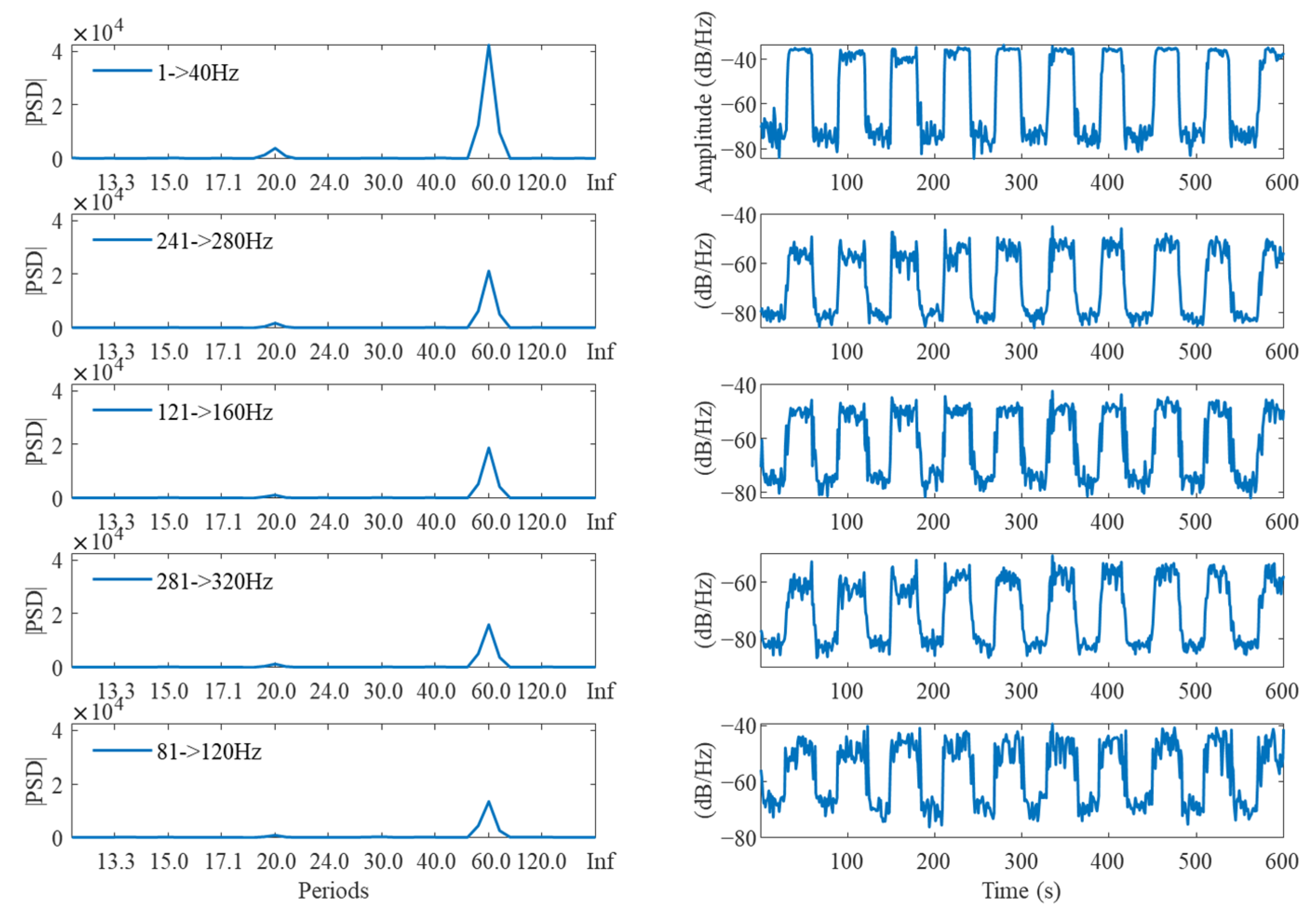
As aforementioned, one of the main motivations behind the oscillatory workload is to assist in the ranking of the frequency bins. In this experiment, the periodicity of the workload was 1 min, or 60 s. As such, the largest magnitude of the PSD for the germane frequency bins will be at 60 s. As shown in Figure 11, the top five ranked frequency bins corresponding to the balanced measurements were presented. These signals were deemed to be the optimum narrow-band signals to include in the subsequent time-series machine learning monitoring.

5.3.3. MSET Training and Surveillance

The final step was to apply the MSET to the signals to generate a model for the predictive maintenance on the incoming measurements. Generally, the 20 frequencies determined from the healthy state measurements from an asset would be the training data for the MSET. This model is used to monitor the new data for the same asset as it changes over time. In this study, an assessment of the VRS process in combination with MSET was conducted to illustrate the value for the predictive monitoring of the fan data.

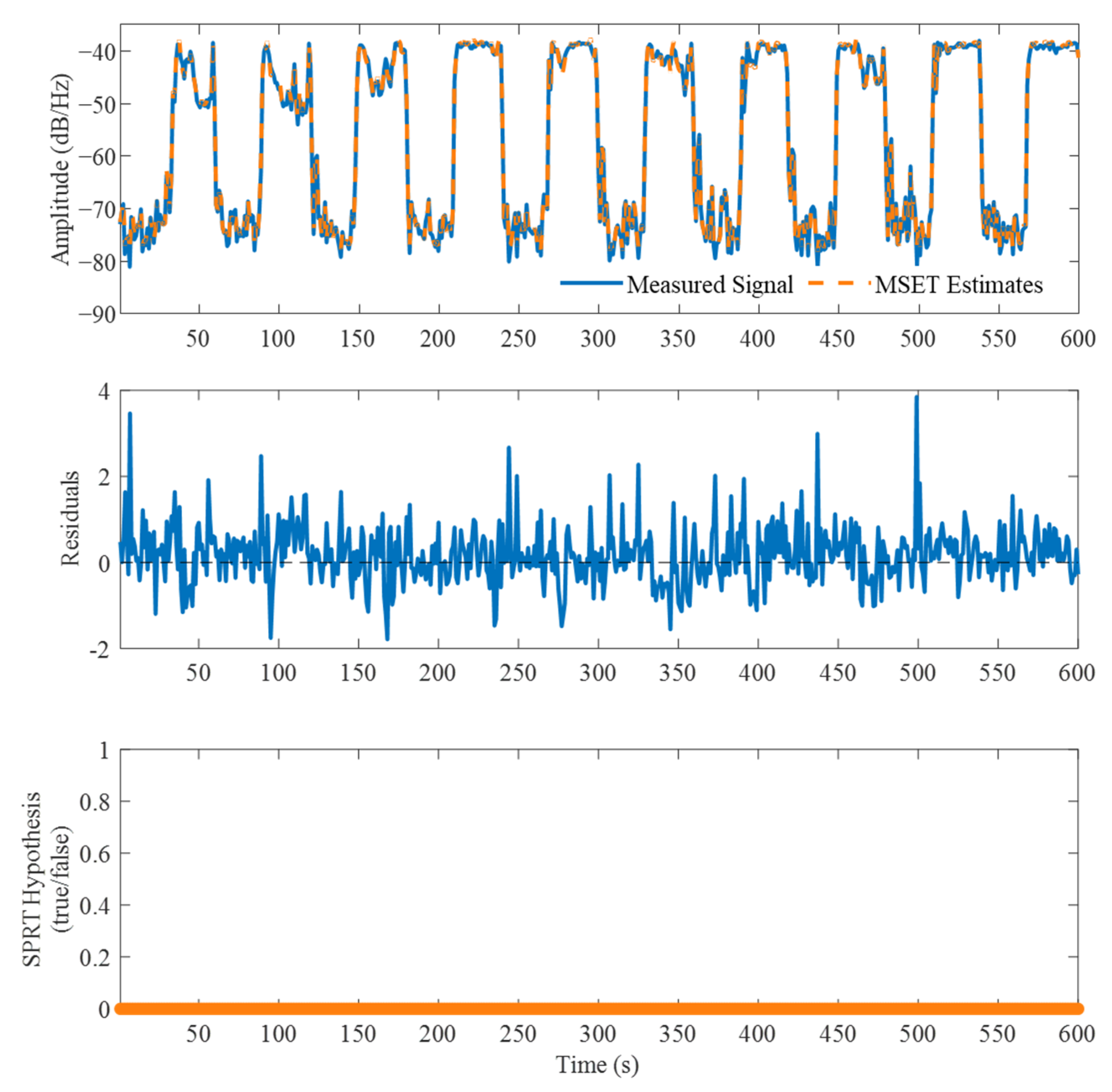
Initially, the prominence of false alarms for the healthy system was determined by evaluating the false alarm probability (FAP) and the variability between measurements. To calculate the FAP, the MSET was first trained on one set of healthy state measurements and was then used to monitor another set. The frequencies chosen for the monitored measurements were the same frequency indexes chosen for the training set. To illustrate the operation of the MSET, an example was given whereby the first set of measurements on the healthy fan model was used to monitor the second set of healthy state measurements, as presented in Figure 12. In the top plot, the generated MSET estimates (orange) were compared with the actual measurements (blue). Subsequently, the residual was calculated as presented in the second subplot to determine the difference between the estimates and the measurements. The SPRT test was then applied to determine the time point at which a deviation in the distribution of the residuals has occurred. Lastly, the results from the SPRT test were presented in the bottom subplot as a binary indicator for the SPRT alerts where 0 indicates “healthy” and 1 indicates “damaged”, respectively. As expected, there was found to be no indication of any degradation, and therefore the FAP for this signal was 0. The FAP is defined as the total sum of SPRT alerts divided by the total SPRT decisions made over the monitoring period.

To assess the reproducibility of the VRS method, a methodical, iterative evaluation whereby all possible permutations of the training and monitoring of the healthy state measurements were conducted. For example, the MSET was trained on the first set of healthy measurements, generating a model that monitored all the remaining sets of measurements. This process was repeated until all four sets of healthy measurements were trained with the MSET and monitored the remaining measurement sets. To assess the quality of the model and the VRS process, the FAP was calculated for each of the 20 frequencies and then averaged. The target FAP in this case was 0.01, which is the expected maximum for any given dataset without degradation. In practice, if the data used to train a MSET model properly encapsulates the dynamics of the system being monitored, the FAP is therefore empirically much lower than the target FAP defined in the SPRT. Therefore, a FAP lower than 0.01 indicates that the model sufficiently emulates the dynamics of the test data and will trigger alarms unnecessarily.

In

Table 1. Average FAP value for the balanced fan models.

Training/Testing	Set 1	Set 2	Set 3	Set 4
Set 1	/	0.0081	0.0040	0.0095
Set 2	0.0076	/	0.0026	0.0135
Set 3	0.0099	0.0026	/	0.0015
Set 4	0.0077	0.0058	0.0034	/

, the averaged FAP values for each training and test case are presented. In all instances, the averaged FAP across all 20 frequencies was lower than the target value of 0.01 except for one instance, which could be attributed to the low sample rate possibly diminishing the capacity for system operational frequency discrimination. Another possibility is that more training data is required. Considering the FAP was found to be lower than the target FAP for the remaining scenarios, the most reasonable explanation for the outlier is the fact that the fan was controlled manually rather than with a program.

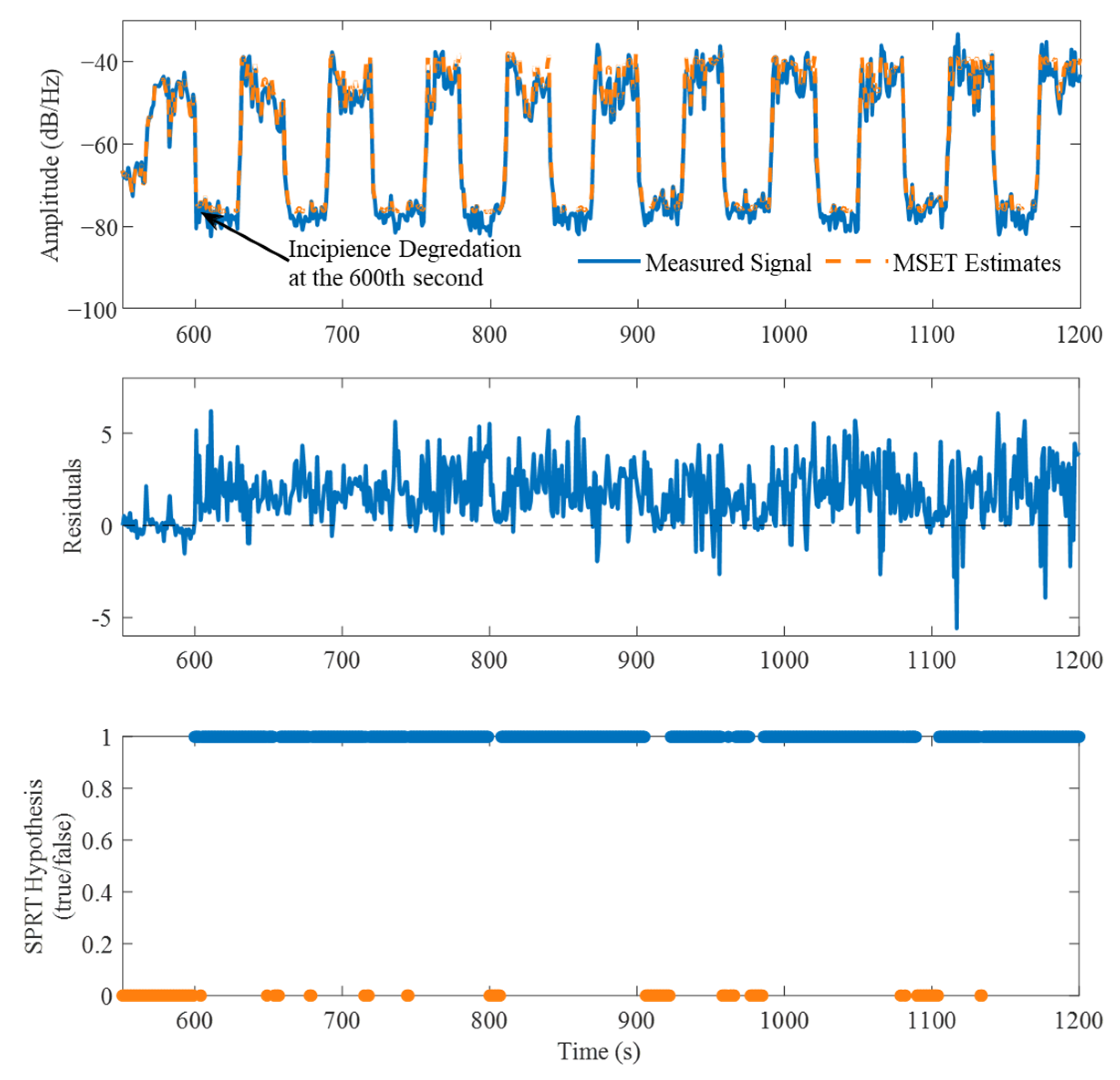
The final step in the process was to utilize the MSET for predictive monitoring. First, the 20 frequencies from the healthy state measurements were determined from the VRS process. Then, the same 20 frequency bin indexes determined from the healthy state were used for the damaged state and concatenated the healthy measurements with the damaged ones. The concatenated signals were intended to simulate a system that suddenly begins to be degraded. The resulting dataset was 20 min of measurements across 20 frequency bins. The MSET was trained on the first 540 s and then monitors for the remaining 660 s. One minute of the healthy measurements remained in the testing phase to illustrate the differentiation capacity of the model. The monitoring stage is presented in Figure 13 with one example signal from the unbalanced set of measurements with the lightest weight. As with the healthy state example, the results include the signal measurements and estimates, the residuals between the two, and the results from the SPRT. The unbalanced measurements were introduced to the testing phase at the 600 s. The MSET can detect this sudden change in operation, as indicated by the SPRT alarms (blue) in the bottom subplot. Then, the weight of the imbalance gradually increased, and each weight imbalance was measured five times. The fan unbalance was calculated by the unbalanced mass multiplied by its distance to the center of the fan divided by the fan mass:

$$\begin{array}{c}e=\frac{m_u\times r}{m_f}\end{array}$$

(2)

where $m_u$ is the unbalanced mass, $r$ is the distance between the center of the fan and the unbalanced mass, and $m_f$ is the mass of the fan.

The confidence factor (or CF) is a ratio between the frequency of triggered alerts, which is indicated by when the SPRT is counter to the null hypothesis ($H_1$), and the number of SPRT decisions, which is defined as when either the null hypothesis ($H_0$) or the counter is confirmed. It is defined by the equations below:

$$\begin{array}{c}SPR{T}_{alert}=H_1=\left\{SPR{T}_{pos}, SPR{T}_{neg}, SPR{T}_{nom}, SPR{T}_{inv}\right\}\end{array}$$

(3)

$$\begin{array}{c}SPR{T}_{decision}=\left\{H_0, H_1\right\}\end{array}$$

(4)

$$\begin{array}{c}CF=\frac{Y_i}{D_i}=\frac{{{\displaystyle \sum }}_{j=1}^{i}SPR{T}_{aler{t}_j}}{{{\displaystyle \sum }}_{j=1}^{i}SPR{T}_{decisio{n}_j}}\end{array}$$

(5)

whereby $SPR{T}_{pos}$, $SPR{T}_{neg}$, $SPR{T}_{nom}$, and $SPR{T}_{inv}$ are all indications of when the mean of the distribution of the residuals have shifted positively or negatively, or when the variance in the residual distribution has increased or decreased, respectively. $SPR{T}_{alert}=\left\{0,1\right\}$ and $SPR{T}_{decision}=\left\{0,1\right\}$ are SPRT output for the $j^{th}$ element of the time series, and the ratio of the cumulative sum of the $SPR{T}_{alert}$ and $SPR{T}_{decision}$ is the confidence factor at each time stamp [20].

Several metrics were tracked, averaged, and presented in

Table 2. Average of the key metrics utilized in the predictive modeling of the damaged assets.

Training/Testing	TTD (s)	Confidence Factor (%)	Fault Found
$e=$ 0.113	53.3	80.78	Yes
$e=$ 0.225	53.2	80.21	Yes
$e=$ 0.338	53.5	88.30	Yes
$e=$ 0.451	53.3	90.73	Yes

. The first metric was the time to detect (TTD) which is particularly important to predictive monitoring. This metric is a description of the capacity of a model to quickly indicate the onset of degradation so it can remediate before it becomes disastrous. The TTD is the first timestamp that indicates where there is a fault. On the average MSET, the predictive modeling system determined that there was degradation approximately 6 s before the degradation began in all cases across all the measurement sets. The reason that detection was possible before the 60th second was because the analysis was run as a static case and not in real time. The SPRT has a secondary function that utilizes a buffer whereby future timestamps and the current timestamp can be assessed at the same time. In a real-time scenario, the buffer size would be adjusted to the latency requirements of the use case. If in this instance the latency requirement was 1 s, the detection would occur instantaneously at 60 s, but not before. Another metric that is useful is the confidence factor. This is a measure of certainty that a fault exists and a proxy for the severity of the fault. The confidence factor is calculated from the cumulative total of alarms by the current index of the time stamp, and is a measure of alarm frequency. The final value in the monitoring phase will result in the maximum confidence factor. The highest confidence factor on any given signal is used to calculate the average. Overall, the MSET was relatively confident in that a fault existed. If the faulty time series signals were longer, the confidence factor would have increased. Lastly, an indication of the fault was recorded, and in all instances for each weight, an imbalance was detected.

Figure 13. Visualization of the MSET monitoring of the unbalanced fan at the frequency of 1.55 kHz.

Figure 13. Visualization of the MSET monitoring of the unbalanced fan at the frequency of 1.55 kHz.

6. Conclusions and Future Directions

In this paper, the vibration resonance spectrometry (VRS) technique, along with an advanced ML signal-processing innovation termed the multivariate state estimation technique (MSET) was applied to detect the unbalance state of a fan model. The main conclusions are given as follows:

(1) The utilization of the novel VRS preprocessing algorithm allows for better predictive monitoring that could be processed with on-premise edge devices or eventually a cloud platform due to its capacity for loss-less dimension reduction;

(2) The process transforms a noisy univariate vibration signal into 20 highly correlated signals that can be used in a multivariate ML model to predict the frequency signature;

(3) The multivariate ML model with the mechanical state of system based on working conditions improve the accuracy of diagnosis thresholds;

(4) When the VRS is placed upstream of the MSET, the real-time condition monitoring becomes more sensitive to the current condition and the onset of degradation or mechanical assists than is currently available in the industry.

In the current test setup, only radial unbalance was considered, and the weights were relatively large. As the next step, the sensitive to the imbalance severity and different types of imbalance will be tested. In addition, the current methodology will be applied to monitor much more complex systems to determine the capacity for root cause analysis, such as a powertrain system. Different types of faults, such as motor winding faults, broken rotor bar, crack gear tooth, and bearing faults will be introduced both individually and together to test the system capability of fault detection.

References

- Niewczas, P.; Dziuda, L.; Fusiek, G.; McDonald, J.R. Design and evaluation of a preprototype hybrid fiber-optic voltage sensor for a remotely interrogated condition monitoring system. IEEE Trans. Instrum. Meas. 2005, 54, 1560–1564. [Google Scholar] [CrossRef]
- Niewczas, P.; Fusiek, G.; McDonald, J.R. Dynamic capabilities of the hybrid fiber-optic voltage and current sensors. In Proceedings of the SENSORS, Daegu, Republic of Korea, 22–25 October 2006; pp. 295–298. [Google Scholar]
- Rabbi, S.F.; Rahman, M.A.; Butt, S.D. Modeling and operation of an interior permanent magnet motor drive for electric submersible pumps. In Proceedings of the 2014 Oceans, St. John’s, NL, Canada, 14–19 September 2014; pp. 1–5. [Google Scholar]
- Da Silva, P.A.S.; da Costa, C.T.; Barreiros, J.A.L. Intelligent Analysis Program Applied to Production Logs in Oil and Gas Wells. IEEE Lat. Am. Trans. 2006, 4, 353–358. [Google Scholar] [CrossRef]
- Shanbr, S.; Elasha, F.; Elforjani, M.; Teixeira, J.A. Bearing fault detection within wind turbine gearbox. In Proceedings of the 2017 International Conference on Sensing, Diagnostics, Prognostics, and Control (SDPC), Shanghai, China, 16–18 August 2017; pp. 565–570. [Google Scholar]
- Yang, J.; Zhao, L.; Lang, Z.-Q.; Zhang, Y. Wind Turbine Blade Condition Monitoring and Damage Detection by Image-Based Method and Frequency-Based Analysis. In Proceedings of the 2018 10th International Conference on Modelling, Identification and Control (ICMIC), Guiyang, China, 2–4 July 2018; pp. 1–6. [Google Scholar]
- Chikuruwo, M.N.H.; Maregedze, L.; Garikayi, T. Design of an automated vibration monitoring system for condition based maintenance of a lathe machine (Case study). In Proceedings of the 2016 International Conference on System Reliability and Science (ICSRS), Paris, France, 15–18 November 2016; pp. 60–63. [Google Scholar]
- Seo, J. A practical scheme for vibration signal measurement-based power transformer on-load tap changer condition monitoring. In Proceedings of the 2018 Condition Monitoring and Diagnosis (CMD), Perth, Australia, 23–26 September 2018; pp. 1–4. [Google Scholar]
- Rikardo, S.A.; Bambang, C.B.; Sumaryadi, C.; Yulian, T.D.; Arief, S.E.; Kharil, S.F.I. Vibration monitoring on power transformer. In Proceedings of the 2008 International Conference on Condition Monitoring and Diagnosis, Beijing, China, 21–24 April 2008; pp. 1015–1016. [Google Scholar]
- Pavithra, R.; Ramachandran, P. An Overview of Predictive Maintenance for Industrial Machine Using Vibration Analysis. In Proceedings of the 2021 Innovations in Power and Advanced Computing Technologies (i-PACT), Kuala Lumpur, Malaysia, 27–29 November 2021; pp. 1–7. [Google Scholar]
- Minaiepour, H.; Sarabeigi, H.; Heydari, E. Surveying compressor C-2501 vibration problem by analysis of vibration and its analytical report. In Proceedings of the 2012 IEEE International Conference on Condition Monitoring and Diagnosis, Bali, Indonesia, 23–27 September 2012; pp. 706–709. [Google Scholar]
- Mo, Y.-C.; Su, K.-Y.; Kang, W.-B.; Chen, L.-B.; Chang, W.-J.; Liu, Y.-H. An FFT-based high-speed spindle monitoring system for analyzing vibrations. In Proceedings of the 2017 Eleventh International Conference on Sensing Technology (ICST), Sydney, Australia, 4–6 December 2017; pp. 1–4. [Google Scholar]
- Ewert, P.; Kowalski, C.T.; Jaworski, M. Comparison of the Effectiveness of Selected Vibration Signal Analysis Methods in the Rotor Unbalance Detection of PMSM Drive System. Electronics 2022, 11, 1748. [Google Scholar] [CrossRef]
- Gangsar, P.; Pandey, R.K.; Chouksey, M. Unbalance detection in rotating machinery based on support vector machine using time and frequency domain vibration features. Noise Vib. Worldw. 2021, 52, 75–85. [Google Scholar] [CrossRef]
- Rahman, M.d.M.; Uddin, M.N. Online Unbalanced Rotor Fault Detection of an IM Drive Based on Both Time and Frequency Domain Analyses. IEEE Trans. Ind. Appl. 2017, 53, 4087–4096. [Google Scholar] [CrossRef]
- Puerto-Santana, C.; Ocampo-Martinez, C.; Diaz-Rozo, J. Mechanical rotor unbalance monitoring based on system identification and signal processing approaches. J. Sound Vib. 2022, 541, 117313. [Google Scholar] [CrossRef]
- Yang, Y.; Dorn, C.; Mancini, T.; Talken, Z.; Kenyon, G.; Farrar, C.; Mascareñas, D. Blind identification of full-field vibration modes from video measurements with phase-based video motion magnification. Mech. Syst. Signal Process. 2017, 85, 567–590. [Google Scholar] [CrossRef]
- Lado-Roigé, R.; Font-Moré, J.; Pérez, M.A. Learning-based video motion magnification approach for vibration-based damage detection. Measurement 2023, 206, 112218. [Google Scholar] [CrossRef]
- Scislo, L. Single-Point and Surface Quality Assessment Algorithm in Continuous Production with the Use of 3D Laser Doppler Scanning Vibrometry System. Sensors 2023, 23, 1263. [Google Scholar] [CrossRef] [PubMed]
- Gross, K.C.; Lu, W. Early detection of signal and process anomalies in enterprise computing systems. In Proceedings of the ICMLA, Las Vegas, NA, USA, 24–27 June 2002; pp. 204–210. [Google Scholar]
- Durgam, S.; Bawankule, L.N.; Khindkar, P.S. Prediction of Fault Detection Based on Vibration Analysis for Motor Applications. In Proceedings of the 2021 4th Biennial International Conference on Nascent Technologies in Engineering (ICNTE), Navi Mumbai, India, 15–16 January 2021; pp. 1–5. [Google Scholar]
- Yuan, X.; Gao, Z.; Tang, K.; Zeng, M.; Wang, Y. Wind turbine gearbox condition monitoring system based on vibration signal. In Proceedings of the 2015 12th IEEE International Conference on Electronic Measurement & Instruments (ICEMI), Qingdao, China, 16–18 July 2015; Volume 1, pp. 159–163. [Google Scholar]
- Sharma, R.; Pandey, N. A neural network model for electric submersible pump surveillance. In Proceedings of the 2016 International Conference on Communication and Signal Processing (ICCSP), Melmaruvathur, India, 6–8 April 2016; pp. 2083–2088. [Google Scholar]
- Gross, K.C.; Baclawski, K.; Chan, E.S.; Gawlick, D.; Ghoneimy, A.; Liu, Z.H.; Zhang, X. MSET Prognostics for Operator Decision Aid for Human-in-the-Loop Supervisory Control Applications. In Proceedings of the 2016 IEEE International Multi-Disciplinary Conference on Cognitive Methods inSituation Awareness and Decision Support (CogSIMA), San Diego, CA, USA, 21–25 March 2016. [Google Scholar]
- Gross, K.C.; McMaster, S.; Porter, A.; Urmanov, A.; Votta, L.G. Proactive system maintenance using software telemetry. In Proceedings of the 1st International Conference on Remote Analysis and Measurment of Software Systems (RAMSS), Portland, OR, USA, 3–10 May 2003; pp. 24–26. [Google Scholar]
- Gross, K.C.; Humenik, K.E. Sequential probability ratio test for nuclear plant component surveillance. Nucl. Technol. 1991, 93, 131–137. [Google Scholar] [CrossRef]
- Wetherbee, E.R.; Wang, G.C.; Gross, K.C.; Dayringer, M.; Lewis, A.; Gerdes, M.T. Counterfeit Device Detection Using EMI Fingerprints. US Patent 11,460,500, 2022. [Google Scholar]
- Durbhaka, G.K.; Selvaraj, B. Predictive maintenance for wind turbine diagnostics using vibration signal analysis based on collaborative recommendation approach. In Proceedings of the 2016 International conference on advances in computing, communications and informatics (ICACCI), Manipal, India, 21–24 September 2016; pp. 1839–1842. [Google Scholar]
- Patil, S.S.; Gaikwad, J.A. Vibration analysis of electrical rotating machines using FFT: A method of predictive maintenance. In Proceedings of the 2013 Fourth International Conference on Computing, Communications and Networking Technologies (ICCCNT), Tiruchengode, India, 4–6 July 2013; pp. 1–6. [Google Scholar]
- Nivesrangsan, P.; Jantarajirojkul, D. Bearing fault monitoring by comparison with main bearing frequency components using vibration signal. In Proceedings of the 2018 5th International Conference on Business and Industrial Research (ICBIR), Bangkok, Thailand, 17–18 May 2018; pp. 292–296. [Google Scholar]