Article

Industrial Process Monitoring Based on Parallel Global-Local Preserving Projection with Mutual Information

1
College of Automation, Chongqing University, Chongqing 400044, China
2
Cloudwalk, Chongqing 401320, China
3
Chongqing Chuanyi Automation Co., Ltd., Chongqing 401121, China
*
Author to whom correspondence should be addressed.
Machines 2023, 11(6), 602; https://doi.org/10.3390/machines11060602
Submission received: 25 April 2023 / Revised: 20 May 2023 / Accepted: 23 May 2023 / Published: 1 June 2023
(This article belongs to the Special Issue Advanced Data Analytics in Intelligent Industry: Theory and Practice)

Abstract

:
This paper proposes a parallel monitoring method for plant-wide processes by integrating mutual information and Bayesian inference into a global-local preserving projections (GLPP)-based multi-block framework. Unlike traditional multivariate statistic process monitoring (MSPM) methods, the proposed MI-PGLPP method transforms plant-wide monitoring into several sub-block monitoringtasks by fully taking advantage of a parallel distributed framework. First, the original datasets of the process are divided into a group of data blocks by quantifying the mutual information of process variables. The block indexes of new data are generated automatically. Second, each data block is modeled by the GLPP method. The variable information and local structure are well preserved during the whole projection. Third, Bayesian inference is introduced to generate final statistics of the process by the probability framework. To illustrate the algorithm performance, a detailed case study is performed on the Tennessee Eastman process. Compared with the principle component analysis and GLPP-based method, the proposed MI-PGLPP provides higher FDRs and superior performance for plant-wide process monitoring.

1. Introduction

With the rapid development of information technology, intelligent sensors are widely applied to industrial manufacturing processes. For this reason, advanced monitoring systems such as SCADA and IIoT are adopted to retrieve real-time data. Process monitoring has become an emerging concern for researchers and industrial engineers [1,2]. Statistical methods have been intensively researched and applied to multivariate statistical process monitoring (MSPM) [3]. The most common practice is to extract process features with dimension reduction methods, then construct a latent variable model for dynamic industrial process monitoring [4]. These methods are based on partial least-squares (PLS) [5], PCA [6], canonical correlation analysis (CCA) [7], Fisher discriminant analysis (FDA) [8], independent component analysis (ICA) [9] and subspace-aided approach [10] etc. These methods and their variants are used to monitor linear, nonlinear, time-variant and multi-mode processes. To further investigate the performance, Shen et al. presented a review [11] to compare the performance of the aforementioned methods on the same industrial process.
Most of the traditional methods focus on solving the MSPM problem by generating latent variables from either global information or local structure, i.e., PCA-based methods use the variance of the dataset to generate projection directions. Meanwhile, a trend of preserving both global and local structures was observed in recent works [12]. The global-local structure analysis (GLSA) [13] model is first applied to monitoring plant-wide processes, which shows promising application prospects. On the basis of the GLSA model, Luo L et al. presented GLPP [4] for industrial process monitoring and kernel GLPP (KGLPP) [14] for nonlinear process monitoring. Their research further analyzes the intrinsic relationship between PCA and LPP, revealing its performance theoretically. Similarly, the FDA is introduced into GLPP in [3] to enhance the fault-identification performance by maximizing scattering between classes and minimizing scattering within classes. Huang et al. [15] proposed the KGLPP-Cam model with a new weighted distance named Cam weighted distance. This approach is used to reselect the neighbors and consequently overcome the non-uniform distributed characteristic of data. For the dynamic process monitoring problems, Tang et al. [16] proposed a hybrid framework by integrating canonical variate analysis into GLPP.
Recently, plant-wide process monitoring is becoming a hot issue and has attracted a lot of researchers’ interests. The multi-block methods are presented to generate sub-blocks of the original dataset, which contributes to significant performance improvement. In general, the multi-block methods consist of three major steps:
  • Block division. The industrial process data are divided into several blocks by certain strategies, i.e., mutual information [17] or knowledge-based methods [18].
  • Block modeling. Each block is modeled by related methods, i.e., PLS, PCA, ICA, etc.
  • Statistics fusion. For an online dataset, several groups of statistics are generated by a well-trained monitoring model. In order to obtain consistent monitoring results, a flexible fusion strategy is required to generate the final statistic pair. According to the literature review, Bayesian inference and voting methods are the common strategies for plant-wide process monitoring.
Based on these steps, researchers have presented several application results. A distributed PCA (DPCA) method [19] is presented, which evolves into the distributed framework presented in paper [20]. This idea is also extended to big data applications [21] and quality monitoring [1]. For the purpose of utilizing process knowledge, a hierarchical hybrid DPCA framework is presented by introducing a knowledge-based strategy and mutual information [18]. For non-Gaussian industrial process monitoring, a multi-block ICA [22] is developed and applied to industrial processes. These data-driven methods have the capability to automatically divide the process into several sub-blocks. However, they are based on covariance and are subject to linear constraints. Process decomposition, as a crucial step in multi-block methods, holds significant importance for practical nonlinear fault detection and diagnosis.
Furthermore, a significant portion of research has been focused on the application of Bayesian methods for industrial process monitoring. For instance, Huang and Yan [23] proposed a dynamic process monitoring method based on DPCA, DICA and Bayesian inference. Jiang et al. [24] established a Bayesian diagnostic system based on optimal principal components (OPCs), enabling probabilistic fault identification. Zou et al. [25] employed Bayesian inference criteria for online performance assessment. Bayesian networks are commonly employed in industrial process monitoring to model dependencies and interactions among process variables, sensors and equipment [26]. Bayesian networks provide a systematic approach to handle uncertainty, identify causal relationships and propagate the effects of changes or faults throughout the entire system [27]. For most modern industrial processes, comprehending and evaluating multiple monitoring outcomes from different units or components using Bayesian techniques holds significant importance. However, Bayesian methods necessitate sufficient data for effective inference and updating, and their successful application relies on appropriate model selection and parameter configuration.
Inspired by the distributed PCA framework [20] and mutual information-based block division [17], a mutual information-based parallel GLPP method (MI-PGLPP) is proposed for plant-wide process monitoring in this paper. With the integration of mutual information, GLPP and Bayesian fusion in a multi-block framework, the advantages of MI-PGLPP are as follows:
  • MI-PGLPP utilizes mutual information of the variables and divides data blocks automatically, which does not require prior knowledge of the process.
  • MI-PGLPP naturally meets the independent condition of Bayesian inference since variables in each block are divided by the independence of mutual information.
  • MI-DGLPP utilizes GLPP to obtain the latent matrix and transformation matrix of each data block. The intrinsic features of global and local structures are well preserved during the projection.
This paper consists of five sections. The rest is organized as follows: Section 2 briefly reviews the fundamental theory of the GLPP method and mutual information in MI-PGLPP. Section 3 presents the detail of MI-PGLPP for process monitoring. Section 4 gives a case study to evaluate the performance of the proposed method. Finally, Section 5 concludes the paper.

2. Preliminaries

This section presents a brief theoretical review of the GLPP method and mutual information. These two methods are integrated into the proposed MI-PGLPP method. The detailed information can be seen in the following parts.

2.1. Global-Local Preserving Projection

Benefiting from the dimensionality-reduction and feature-extraction capabilities of PCA and LPP, these two methods are often used in industrial process inspection to project original datasets into a low-dimensional space. During the data projection procedure, PCA preserves the variance information while LPP keeps the local neighborhood structure information [4]. Therefore, these two methods and their variants may lead to information loss when performing data projection. Unlike these methods, the GLSA-based [13] method aims to generate the spatial correlations of original datasets by preserving the variance and local structure information [3]. For a given dataset X = x 1 , x 2 , , x n R m × n with n samples and m variables, GLPP formulates a projection matrix A R m × k and projects X into lower-dimensional data Y = y 1 , y 2 , , y k R k × n ( k m ) ,
y i = A T x i Y = A T x
In order to retain the global and adjacent structures of dataset X , the objective function is formulated as follows [4,13]
J G L P P ( a ) = min a J Local ( a ) , J G l o b a l ( a ) J Local ( a ) = 1 2 i j y i y j 2 W i j J G l o b a l ( a ) = 1 2 i j y i y j 2 W ¯ i j
where a denotes the transformation vector and y i T = a T X , adjacent matrix W i j and nonadjacent weighting matrix W ¯ i j are defined as follows [4,13,28].
W i j = e x i x j 2 σ 1 , if x j Ω k x i or x i Ω k x j 0 , otherwise
W ¯ i j = e x i x j 2 σ 2 , if x j Ω k x i or x i Ω k x j 0 , otherwise
where σ 1 and σ 2 are constant parameters and Ω k x i denotes the k nearest neighbors of data point x i . It is easy to find out that σ 1 and σ 2 are both in the interval [ 0 , 1 ] . Equation (2) can be reformulated as [3,4]
J G L P P ( a ) = min a η J G l o b a l ( a ) ( 1 η ) J Local ( a ) = min a 1 2 η i j y i y j 2 W i j ( 1 η ) i j y i y j 2 W ¯ i j
where η is the tradeoff between global and local information in projection.
With some basic arithmetic operations, Equation (5) can be written as,
J G L P P = min a i j y i y j 2 R i j = min a a T X ( H R ) X T a = min a a T X M X T a
where R i j = η W i j ( 1 η ) W ¯ i j , H is a diagonal matrix with H i j = j R i j and M = H R denotes the Laplacian matrix [4].
Furthermore, a common constraint is introduced to transform the above objective function into a constrained optimization problem [15,16],
min a a T X M X T a s . t . a T N a = 1
where N = η X H X T + ( 1 η ) I and I denotes identity matrix.
It is easy to transform Equation (7) into a generalized eigenvalue problem,
X M X T a = λ X N X T a
By solving Equation (8), the transformation matrix A is finally obtained by the k-th eigenvectors a 1 , a 2 , , a k which correspond to the eigenvalues λ 1 , λ 2 , , λ k .

2.2. Mutual Information

Mutual information is defined as a non-parametric index [17] and used to quantify the mutual dependence of variables from the perspective of entropy [29]. For given vectors x 1 and x 2 , the mutual information M I is defined with the aid of the joint probability density function [30],
M I ( x 1 , x 2 ) = x 1 , x 2 p j ( x 1 , x 2 ) log p j ( x 1 , x 2 ) p m ( x 1 ) , p m ( x 2 ) d x 1 d x 2
where p m ( x 1 ) and p m ( x 2 ) denote marginal probability of x 1 and x 2 , respectively. p j ( x 1 , x 2 ) represents the joint probability density function of variable x 1 and variable x 2 .
By introducing Shannon entropy, Equation (9) can be clarified as follows [31]:
M I ( x 1 , x 2 ) = H j ( x 1 ) + H j ( x 2 ) H m ( x 1 , x 2 )
where H j ( x 1 , x 2 ) is the joint entropy of x 1 and x 2 , the Shannon entropy of x can be defined as [32]:
H j ( x ) = x p j ( x ) log p j ( x ) d x
Similarly, the joint entropy H m ( x 1 , x 2 ) can be defined as [31]:
H m ( x 1 , x 2 ) = x 1 , x 2 p m ( x 1 , x 2 ) log ( p m ( x 1 , x 2 ) ) d x 1 d x 2
Since mutual information describes the dependence of variables in high-dimensional space, it can be used in both linear and nonlinear analysis. Furthermore, it is obvious that the stronger relevance of two variables leads to larger mutual information.

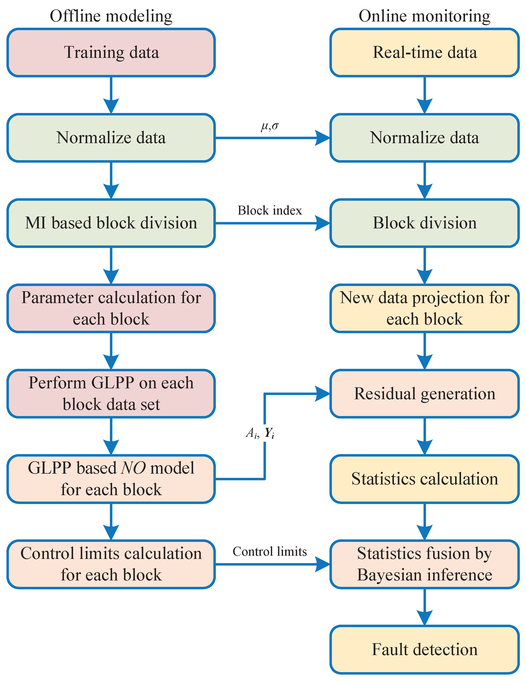
3. Fault Diagnosis Based on MI-PGLPP

This section explains the detail of the proposed MI-PGLPP method. Its framework is shown in Figure 1, which consists of three major steps.
  • Step 1: Block selection. The original dataset is divided into several subblocks.
  • Step 2: Offline model training. The block model is obtained by the subblocks of the dataset.
  • Step 3: Online monitoring. The statistics of each subblock is generated by the online data and the final statistics pair is calculated by fusion strategies.

3.1. Mutual Information-Based Variable Block Division

A large-scale process such as the plant-wide process takes a number of resources to train a universal monitoring model. However, the model does not always perform as well as the initial purpose. Thus, some distributed methods are proposed aiming at a plant-wide monitoring problem [20,21,33]. These methods divide the dataset into several blocks via physical structure analysis, empirical analysis and quantitative calculation. Mutual information is a typical technique of quantitative methods and used in various methods to deal with variable selection problems.
As in papers [17,29], mutual information is introduced to divide the original process data into several data blocks. In each block, the variables have stronger dependence, contributing to fewer model efforts and better data features. For dataset X R m × n , the mutual information M I x i , x j is calculated as Equation (10),
M I x i , x j = M I ( x i , x j )
where i , j 1 , 2 , , m . A numerical example for MI calculation is shown in Figure 2.
The division principle depends on the MI value. For example if M I x i , x j > M I x i , x k , variable x j will be divided into the block with variable x i . The dataset X can be divided into the following blocks,
X = [ X 1 , X 2 , , X N ]
where N denotes the block number, for i [ 1 , 2 , , N ] , X i R m i × n and m i denotes dimension of data block X i .
This step aims to partition the original dataset of the process into a set of data blocks by quantifying the mutual information between process variables. It automatically generates block indices for the new data. Based on the calculation principles of mutual information, a higher MI value indicates stronger dependency between variables, which contributes to reduced modeling effort and improved data characterization.

3.2. GLPP-Based Block Data Modeling

For the i-th data block X i T R n × m i , the offline normal operation model can be trained by GLPP
X i = Y i A i T + E i Y i = X i A i ( A i T A i ) 1 E i = X i Y i A i T
where A i = [ a i 1 , a i 2 , , a m i k ] R m i × m i k denotes the transform matrix, Y i = [ y i 1 , y i 2 , , y m i k ] R n × m i k denotes the latent variable matrix, and matrix E i represents the residual.
For process monitoring of each block, T 2 and S P E statistics are applied to GLPP model and their control limits are defined as follows [34],
T i , l i m i t s 2 = m i k ( n 2 1 ) n ( n m i k ) F α ( m i k , n m i k ) S P E i , l i m i t s = θ 1 1 θ 2 h 0 1 h 0 θ 1 2 + z α ( 2 θ 2 h 0 2 ) θ 1 1 h 0
where m i k is the dimension of latent variables in block i. ∼ F α ( m i k , n m i k ) denotes ∼F-distribution, α is the significance level. h 0 = 1 [ ( 2 θ 1 θ 3 ) / ( 3 θ 2 2 ) ] , θ 2 = t r ( c o v ( E i ) 2 ) , θ 3 = t r ( c o v ( E i ) 3 ) and z α denotes the standardized normal variable with confidence 1 α .
In each block, the monitoring performance depends on the selection of parameter η . In order to meet the requirements of tradeoff between global information and local information in the latent matrix, several feasible principles have been applied according to the dataset. For industrial time series analysis, a spectral radius based approach [4,16] is presented to select parameter η ,
η = δ ( L ¯ ) δ ( L ¯ ) + δ ( L )
where δ ( L ) and δ ( L ¯ ) denote the spectral radius of local and global Laplacian matrices, respectively.
For block i, the new data sample x i n e w R 1 × m i is projected onto the i-th well-trained offline model,
x i n e w = A i y i n e w + e i , n e w y i n e w = ( A i T A i ) 1 A i T x i n e w e i , n e w = x i n e w A i y i n e w
The T i , n e w 2 and S P E i , n e w statistics of the i-th block are calculated as follows,
T i , n e w 2 = y i n e w T ( Y i T Y i n 1 ) 1 y i n e w S P E i , n e w = e i , n e w T e i , n e w
where Y i denotes the i-th latent variable matrix.
For each block, { T i , n e w 2 , S P E i , n e w } i = 1 , 2 , , N are calculated online with new monitoring data. The monitoring results of each block are simply generated by comparing statistics of new sample data with their control limits { T i , l i m i t s 2 , S P E i , l i m i t s } i = 1 , 2 , , N . For example, if T i , n e w 2 > T i , l i m i t s 2 , a process fault is triggered by the T 2 statistics of the i-th block model.
Since there are several blocks, the final monitoring results can be further calculated by some fusion strategies. According to the literature review, the probabilistic framework is the common solution to this problem. The following section introduces a Bayesian inference strategy to generate final monitoring results.

3.3. Bayesian Inference-Based Monitoring Result Fusion

Bayesian inference is prevalent in distributed monitoring such as distributed PCA methods [35], distributed ICA [36] and so on. This section presents Bayesian inference based monitoring result fusion.
Firstly, the normal operation and faulty case are tagged with N and F , respectively. p T 2 i ( N ) and p T 2 i ( F ) , p S P E i ( N ) and p S P E i ( F ) are the prior probabilities of T 2 and S P E statistics of the i-th block corresponding to operation modes N and F , which can be calculated by significance level α and 1 α . The probabilities of T 2 and S P E statistics are determined by
p T 2 i ( x i n e w N ) = e x p T i , n e w 2 T i , l i m i t s 2 p T 2 i ( x i n e w F ) = e x p T i , l i m i t s 2 T i , n e w 2
p S P E i ( x i n e w N ) = e x p S P E i , n e w S P E i , l i m i t s p S P E i ( x i n e w F ) = e x p S P E i , l i m i t s S P E i , n e w
Based on Equations (20) and (21) and prior probabilities, the fault probabilities of data point x i n e w can be calculated as,
p T 2 i ( F x i n e w ) = p T 2 i ( x i n e w F ) p T 2 i ( F ) p T 2 i ( x i n e w ) p S P E i ( F x i n e w ) = p S P E i ( x i n e w F ) p S P E i ( F ) p S P E i ( x i n e w )
where p T 2 i ( x i n e w ) and p S P E i ( x i n e w ) are calculated as
p T 2 i ( x i n e w ) = p T 2 i ( x i n e w N ) p T 2 i ( N ) + p T 2 i ( x i n e w F ) p T 2 i ( F ) p S P E i ( x i n e w ) = p S P E i ( x i n e w N ) p S P E i ( N ) + p S P E i ( x i n e w F ) p S P E i ( F )
With Equation (22), fault probabilities of each block can be calculated corresponding to T 2 and S P E statistics. The probabilities set { p T 2 i ( F x i n e w ) } i = 1 , 2 , , N and { p S P E i ( F x i n e w ) } i = 1 , 2 , , N are further integrated by a weighted probability approach [20],
p T 2 ( F x n e w ) = i = 1 N p T 2 i ( F x i n e w ) p T 2 i ( x i n e w F ) i = 1 N p T 2 i ( F x i n e w ) p S P E ( F x n e w ) = i = 1 N p S P E i ( F x i n e w ) p S P E i ( x i n e w F ) i = 1 N p S P E i ( F x i n e w )
In a Bayesian inference framework, the assumption of independence is essential and requires lower correlation between variables x i and x j . Because sub-blocks are divided by mutual information with low dependence, variables in each sub-block are relatively independent of each other. As a result, fault-monitoring performance is guaranteed to the maximum extent.
Based on the final statistics p T 2 ( F x n e w ) and p S P E ( F x n e w ) , the monitoring result is determined by the significance level α as
NO : p T 2 ( F x n e w ) α & p S P E ( F x n e w ) α FO : p T 2 ( F x n e w ) > α o r p S P E ( F x n e w ) > α
where NO and FO denote normal operation and faulty operation, respectively.

3.4. Monitoring Procedure

The proposed MI-PGLPP based process monitoring can be applied as the procedures in Figure 3.
Step 1: Steps of offline modeling:
  • Normalize each data block by Z-score standardization and generate data mean and variance.
  • Analyze the variable dependence of training dataset by Equation (10), and then generate the data blocks and block index.
  • Construct adjacent weighting matrix W i j and nonadjacent weighting matrix W ¯ i j by Equation (4).
  • Calculate the tradeoff parameter η by Equation (17) for each data block.
  • Perform GLPP on each data block X i by Equation (7) and generate transformation matrices A i , latent matrices Y i and NO model.
  • Define significance level α and calculate control limits for each data block by Equation (16).
Step 2: Steps of online monitoring:
  • Acquire the new sample data x n e w and perform normalization with the mean and variance of training samples.
  • Divide new data x n e w into N blocks with the variable index generated by the training data.
  • Project each block data point on the NO model and generate residual e i , n e w of each block by Equation (18).
  • Calculate the statistics of each block by Equation (19).
  • Calculate the prior probabilities, conditional probabilities and fault probabilities by Equations (20)–(23).
  • Perform statistics fusion with Bayesian inference by Equation (24).
  • Monitor the process by Equation (25).

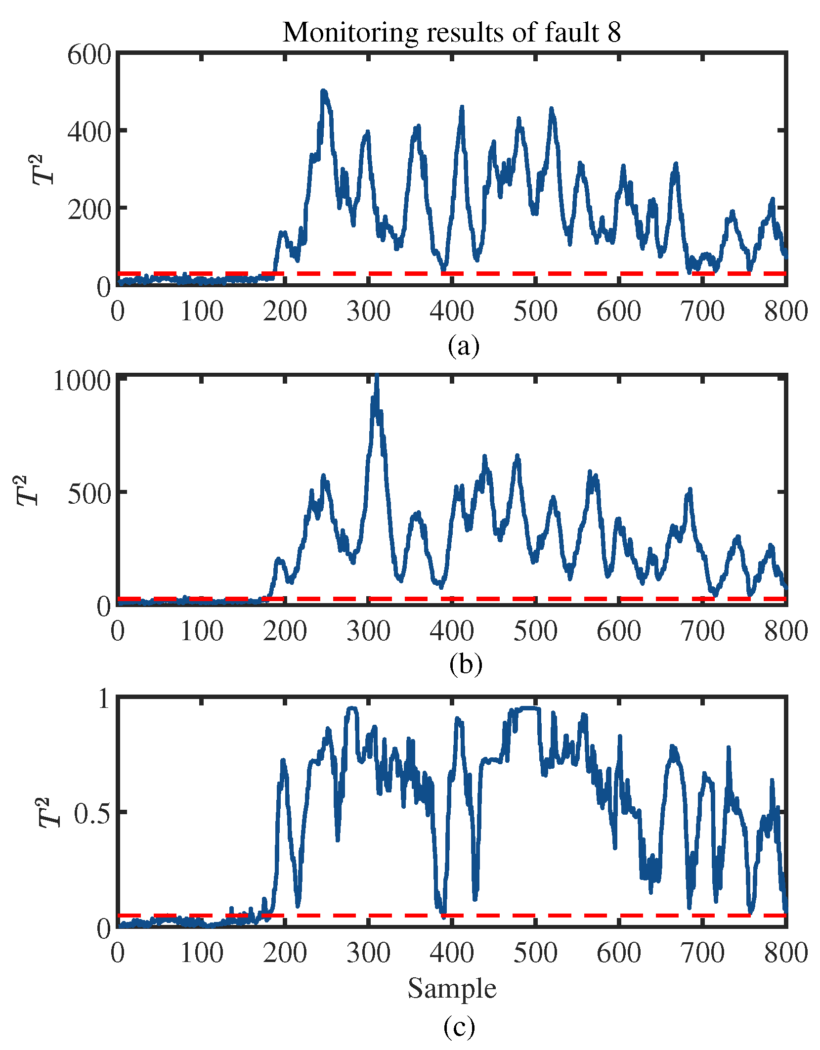
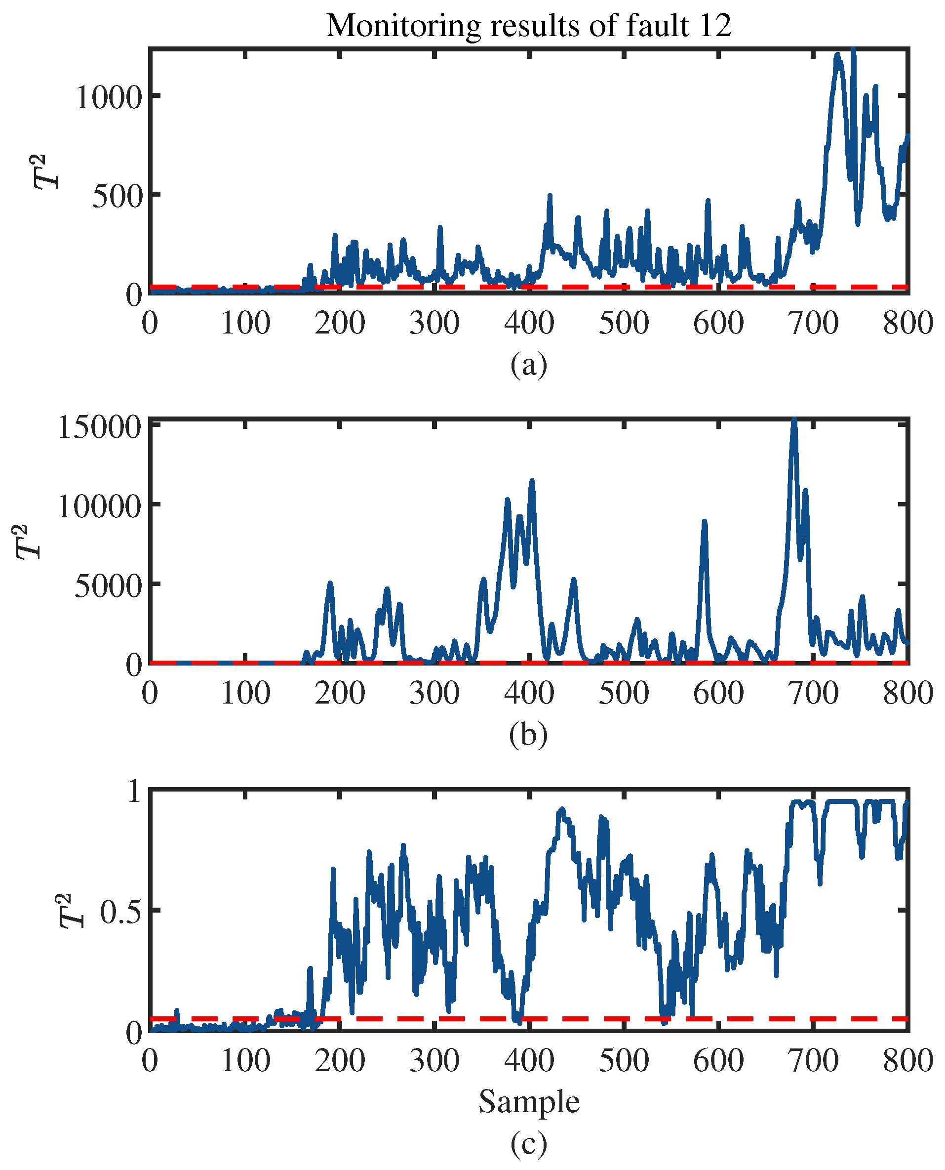
4. Experiments and Results

In this section, the Tennessee Eastman (TE) process [37] is adopted to evaluate the performance of the proposed method. The TE process is a benchmark for data-driven fault diagnosis strategies and is widely applied to illustrating process monitoring performance [11]. It consists of five major process unit [38], including a vapor–liquid flash separator, an exothermic two-phase reactor, a reboiled product stripper, a recycling compressor and a product condenser (mixer) [3]. As shown in Figure 4, the TE process produces two products and a byproduct from four gaseous materials [39].
The Tennessee Eastman process is simulated using mathematical models that capture the behavior of a chemical plant. The simulation involves solving equations based on principles of physics and chemistry to calculate the evolution of process variables over time. The simulation replicates the dynamics of a real chemical plant, considering factors such as reaction kinetics, heat transfer and fluid flow. It allows researchers to analyze the process behavior, evaluate control strategies and test techniques before implementing them in real-world applications.
The TE process has 53 monitored variables, including 22 process variables, 12 manipulated variables and 19 component measurements. In this study, 11 manipulated variables and 22 continuously monitored variables are selected as experimental datasets. A total of 21 faults were obtained under 21 different types of disturbances.
Faults in the TE process are classified into five categories: group 1 is step changes corresponding to faults 1–7, group 2 is random changes corresponding to faults 8–12, group 3 is a slow shift of reaction kinetics corresponding to fault 13, group 4 is unknown faults corresponding to faults 16–20 and the last group is valve sticking, corresponding to faults 14, 15 and 21. More information on faults in the TE process is presented in paper [3,17,40]. The training datasets are acquired under normal operating conditions, which consist of 960 samples, and all variables are collected every three minutes. Then introducing each fault into process at sample 160 to collect the fault datasets.
The normal operation process is utilized as modeling input, and 21 faults are introduced to verify the monitoring performance. For further illustration, the feasibility of MI-PGLPP, PCA and GLPP-based methods are introduced to monitor the TE process. The significance level of three methods is set as α = 0.05 , and the principle contribution rate is set as σ P C A = 0.85 . For the GLPP method, the parameters are referred to paper [3] and selected as neighborhood number k = 10 , local weight σ 1 = 48 , global weight σ 2 = 132 . The proposed MI-PGLPP also utilizes these parameter settings. Furthermore, the neighborhood number is set as k = 2 due to the group characteristics. The mutual-information-based multiblock principal component analysis (MI–MBPCA) [17] and the global DISSIM (GDISSIM) model [41] are also constructed for comparison. During the construction, the window length is set to be 30 by trial and error. A total of 371 moving windows are generated in each test dataset and the fault is introduced from the 172th the moving window. The confidence level is defined as 0.99.
The fault detection rate (FDR), which is widely used for monitoring results evaluation, was also introduced in this study for performance comparison. Since there are two statistical results of the experiment, this study uses a voting strategy to determine the FDR.
F D R = m a x { F D R T 2 , F D R S P E }
where F D R of certain statistics is defined as in Ref. [11],
F D R s t a t i s = C o u n t ( J > J t h FO ) C o u n t ( FO )
In order to construct a multi-block model, the mutual information between each pair of variables was computed. In all, 33 continuous variables are used for process monitoring, represented as x = χ 1 , χ 2 , , χ 33 , which was partitioned into 7 sub-blocks, consisting of 6 typical blocks and 1 unknown block. The variables within each sub-block are listed in Table 1.
According to FDRs in Table 2, the proposed method performs much better for 10 faults. They are fault 1, fault 2, fault 6, fault 7, fault 8, fault 12, fault 13, fault 14, fault 17 and fault 18. It is capable of handling monitor step, slow drift, random variation and unknown fault. The result shows that the proposed MI-PGLPP can cover all types of fault in the TE process.It is also seen that the results seem bad only for Fault 4. The reason may be that the monitoring variables in the Fault 4 are related-fault, which makes it difficult for the original data to divide the block through the mutual information in the proposed method. Moreover, Fault 4 is characterized by unique patterns that are more challenging to detect and classify compared to other faults. The T 2 and S P E statistics can generate alarms for most faults around sample 160 when faults are introduced. Figure 5 and Figure 6 show the performance of MI-DLPP for monitoring fault 1, fault 2 and fault 7. All faults are introduced at sample 160. Both T 2 and S P E statistics can alarm fault occurrence after about four samples.
For the purpose of further exploring the performance of MI-PGLPP, more experimental results are presented below, in Figure 7, Figure 8, Figure 9 and Figure 10. Figure 7 and Figure 8 are the monitoring results of fault 8 whereas Figure 9 and Figure 10 are the detection performance of Fault 12.
Therefore, a higher FDR implies better monitoring performance. The FDRs of three methods are shown in Table 2, and bold numbers indicate optimum performance with certain failures. It is not difficult to see that MI-PGLPP contributes most of the highest FDR even for fault 3, fault 9 and fault 15, which are generally recognized as the most difficult monitoring faults. Moreover, the average FDR of MI-PGLPP is also higher than those of the other two methods.
All methods show acceptable performance on Fault 8, while MI-PGLPP outperforms the other two methods on Fault 12 in this study. These results fully demonstrate the effectiveness of MI-PGLPP for the TE process, which is recognized as a typical benchmark of plant-wide process monitoring applications.

5. Conclusions

In this paper, the MI-PGLPP method is proposed and applied to monitoring plant-wide processes. Different from PCA and GLPP, MI-PGLPP adopts a parallel distributed framework. To uncover the nonlinear characteristics between data blocks, the proposed method combines mutual information with classical GLPP, partitioning high-dimensional datasets into blocks and projecting the local structure and global information of each block into a latent variable space. For process monitoring applications, the new dataset is projected onto the transformation matrices to generate latent matrices and residuals. Leveraging the fully explored data, Bayesian inference is employed to integrate the statistical information of each data block. Ultimately, experimental monitoring of the TE process demonstrates that MI-PGLPP outperforms the other methods in terms of FDR. Further research is needed to reveal the fundamental reasons behind the performance degradation of MI-PGLPP under certain faults, which could contribute to improving the monitoring outcomes for such faults in the future.

Author Contributions

Conceptualization, T.W.; methodology, T.W.; software, T.W.; validation, Z.Y., J.Y. and P.W.; writing—original draft preparation, T.W.; writing—review and editing, Y.Q.; supervision, H.Y. All authors have read and agreed to the published version of the manuscript.

Funding

This research received no external funding.

Data Availability Statement

The data presented in this study are openly available in [37].

Conflicts of Interest

The authors declare no conflict of interest.

References

  1. Yu, W.; Zhao, C.; Huang, B.; Wu, M. A Robust Dissimilarity Distribution Analytics with Laplace Distribution for Incipient Fault Detection. IEEE Trans. Ind. Electron. 2023; early access. [Google Scholar] [CrossRef]
  2. Cai, L.; Yin, H.; Lin, J.; Zhou, H.; Zhao, D. A Relevant Variable Selection and SVDD-Based Fault Detection Method for Process Monitoring. IEEE Trans. Autom. Sci. Eng. 2022; early access. [Google Scholar] [CrossRef]
  3. Tang, Q.; Chai, Y.; Qu, J.; Fang, X. Industrial process monitoring based on Fisher discriminant global-local preserving projection. J. Process Control 2019, 81, 76–86. [Google Scholar] [CrossRef]
  4. Luo, L. Process monitoring with global-local preserving projections. Ind. Eng. Chem. Res. 2014, 53, 7696–7705. [Google Scholar] [CrossRef]
  5. Choi, S.W.; Lee, I.B. Multiblock PLS-based localized process diagnosis. J. Process Control 2005, 15, 295–306. [Google Scholar] [CrossRef]
  6. Zhou, B.; Ye, H.; Zhang, H.; Li, M. Process monitoring of iron-making process in a blast furnace with PCA-based methods. Control Eng. Pract. 2016, 47, 1–14. [Google Scholar] [CrossRef]
  7. Chen, Z.; Ding, S.X.; Zhang, K.; Li, Z.; Hu, Z. Canonical correlation analysis-based fault detection methods with application to alumina evaporation process. Control Eng. Pract. 2016, 46, 51–58. [Google Scholar] [CrossRef]
  8. He, X.B.; Wang, W.; Yang, Y.P.; Yang, Y.H. Variable-weighted Fisher discriminant analysis for process fault diagnosis. J. Process Control 2009, 19, 923–931. [Google Scholar] [CrossRef]
  9. Lee, J.M.; Yoo, C.; Lee, I.B. Statistical process monitoring with independent component analysis. J. Process Control 2004, 14, 467–485. [Google Scholar] [CrossRef]
  10. Ge, Z.; Zhang, M.; Song, Z. Nonlinear process monitoring based on linear subspace and Bayesian inference. J. Process Control 2010, 20, 676–688. [Google Scholar] [CrossRef]
  11. Yin, S.; Ding, S.X.; Haghani, A.; Hao, H.; Zhang, P. A comparison study of basic data-driven fault diagnosis and process monitoring methods on the benchmark Tennessee Eastman process. J. Process Control 2012, 22, 1567–1581. [Google Scholar] [CrossRef]
  12. Huang, J.; Yan, X. Related and independent variable fault detection based on KPCA and SVDD. J. Process Control 2016, 39, 88–99. [Google Scholar] [CrossRef]
  13. Zhang, M.; Ge, Z.; Song, Z.; Fu, R. Global–Local Structure Analysis Model and Its Application for Fault Detection and Identification. Ind. Eng. Chem. Res. 2011, 50, 6837–6848. [Google Scholar] [CrossRef]
  14. Luo, L.; Bao, S.; Mao, J.; Tang, D. Nonlinear process monitoring based on kernel global-local preserving projections. J. Process Control 2016, 38, 11–21. [Google Scholar] [CrossRef]
  15. Huang, C.; Chai, Y.; Liu, B.; Tang, Q.; Qi, F. Industrial process fault detection based on KGLPP model with Cam weighted distance. J. Process Control 2021, 106, 110–121. [Google Scholar] [CrossRef]
  16. Tang, Q.; Liu, Y.; Chai, Y.; Huang, C.; Liu, B. Dynamic process monitoring based on canonical global and local preserving projection analysis. J. Process Control 2021, 106, 221–232. [Google Scholar] [CrossRef]
  17. Jiang, Q.; Yan, X. Plant-wide process monitoring based on mutual information-multiblock principal component analysis. ISA Trans. 2014, 53, 1516–1527. [Google Scholar] [CrossRef] [PubMed]
  18. Cao, Y.; Yuan, X.; Wang, Y.; Gui, W. Hierarchical hybrid distributed PCA for plant-wide monitoring of chemical processes. Control Eng. Pract. 2021, vol. 111, 104784. [Google Scholar] [CrossRef]
  19. Ge, Z.; Song, Z. Distributed PCA Model for Plant-Wide Process Monitoring. Ind. Eng. Chem. Res. 2013, 52, 1947–1957. [Google Scholar] [CrossRef]
  20. Ge, Z.; Chen, J. Plant-Wide Industrial Process Monitoring: A Distributed Modeling Framework. IEEE Trans. Ind. Inform. 2016, 12, 310–321. [Google Scholar] [CrossRef]
  21. Zhu, J.; Ge, Z.; Song, Z. Distributed Parallel PCA for Modeling and Monitoring of Large-Scale Plant-Wide Processes With Big Data. IEEE Trans. Ind. Inform. 2017, 13, 1877–1885. [Google Scholar] [CrossRef]
  22. Jiang, Q.; Wang, B.; Yan, X. Multiblock independent component analysis integrated with hellinger distance and bayesian inference for non-gaussian plant-wide process monitoring. Ind. Eng. Chem. Res. 2015, 54, 2497–2508. [Google Scholar] [CrossRef]
  23. Huang, J.; Yan, X. Dynamic process fault detection and diagnosis based on dynamic principal component analysis, dynamic independent component analysis and Bayesian inference. Chemom. Intell. Lab. Syst. 2015, 148, 115–127. [Google Scholar] [CrossRef]
  24. Jiang, Q.; Huang, B.; Yan, X. GMM and optimal principal components-based Bayesian method for multimode fault diagnosis. Comput. Chem. Eng. 2016, 84, 338–349. [Google Scholar] [CrossRef]
  25. Zou, X.; Zhao, C.; Gao, F. Linearity Decomposition-Based Cointegration Analysis for Nonlinear and Nonstationary Process Performance Assessment. Ind. Eng. Chem. Res. 2020, 59, 3052–3063. [Google Scholar] [CrossRef]
  26. Yu, H.; Khan, F.; Garaniya, V. Modified Independent Component Analysis and Bayesian Network-Based Two-Stage Fault Diagnosis of Process Operations. Ind. Eng. Chem. Res. 2015, 54, 2724–2742. [Google Scholar] [CrossRef]
  27. Gharahbagheri, H.; Imtiaz, S.A.; Khan, F. Root Cause Diagnosis of Process Fault Using KPCA and Bayesian Network. Ind. Eng. Chem. Res. 2017, 56, 2054–2070. [Google Scholar] [CrossRef]
  28. Tang, Q.; Li, B.; Chai, Y.; Qu, J.; Ren, H. Improved sparse representation based on local preserving projection for the fault diagnosis of multivariable system. Sci. China Inf. Sci. 2021, 64, 254–256. [Google Scholar] [CrossRef]
  29. Zeng, J.; Huang, W.; Wang, Z.; Liang, J. Mutual information-based sparse multiblock dissimilarity method for incipient fault detection and diagnosis in plant-wide process. J. Process Control 2019, 83, 63–76. [Google Scholar] [CrossRef]
  30. Jia, Q.; Li, S. Process Monitoring Based on the Multiblock Rolling Pin Vine Copula. Ind. Eng. Chem. Res. 2020, 59, 18050–18060. [Google Scholar] [CrossRef]
  31. Huang, J.; Yan, X. Quality Relevant and Independent Two Block Monitoring Based on Mutual Information and KPCA. IEEE Trans. Ind. Electron. 2017, 64, 6518–6527. [Google Scholar] [CrossRef]
  32. Zhang, X.; Li, Y.; Kano, M. Quality Prediction in Complex Batch Processes with Just-in-Time Learning Model Based on Non-Gaussian Dissimilarity Measure. Ind. Eng. Chem. Res. 2015, 54, 7694–7705. [Google Scholar] [CrossRef]
  33. Qin, Y.; Arunan, A.; Yuen, C. Digital twin for real-time Li-ion battery state of health estimation with partially discharged cycling data. IEEE Trans. Ind. Inform. 2023; early access. [Google Scholar] [CrossRef]
  34. Qin, Y.; Adams, S.; Yuen, C. Transfer learning-based state of charge estimation for Lithium-ion battery at varying ambient temperatures. IEEE Trans. Ind. Inform. 2021, 17, 7304–7315. [Google Scholar] [CrossRef]
  35. Ge, Z.; Song, Z. Bayesian inference and joint probability analysis for batch process monitoring. AIChE J. 2013, 59, 3702–3713. [Google Scholar] [CrossRef]
  36. Tong, C.; Palazoglu, A.; Yan, X. Improved ICA for process monitoring based on ensemble learning and Bayesian inference. Chemom. Intell. Lab. Syst. 2014, 135, 141–149. [Google Scholar] [CrossRef]
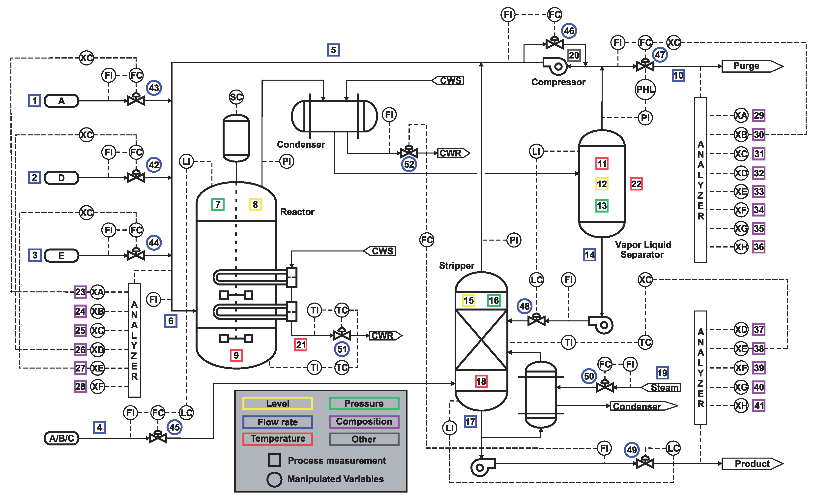
  37. Downs, J.; Vogel, E. A plant-wide industrial process control problem. Comput. Chem. Eng. 1993, 17, 245–255. [Google Scholar] [CrossRef]
  38. Jiang, Q.; Yan, X. Nonlinear plant-wide process monitoring using MI-spectral clustering and Bayesian inference-based multiblock KPCA. J. Process Control 2015, 32, 38–50. [Google Scholar] [CrossRef]
  39. Zhan, C.; Li, S.; Yang, Y. Enhanced Fault Detection Based on Ensemble Global–Local Preserving Projections with Quantitative Global–Local Structure Analysis. Ind. Eng. Chem. Res. 2017, 56, 10743–10755. [Google Scholar] [CrossRef]
  40. Wang, Y.; Fan, J.; Yao, Y. Online Monitoring of Multivariate Processes Using Higher-Order Cumulants Analysis. Ind. Eng. Chem. Res. 2014, 53, 4328–4338. [Google Scholar] [CrossRef]
  41. Zhao, C.; Gao, F. A sparse dissimilarity analysis algorithm for incipient fault isolation with no priori fault information. Control Eng. Pract. 2017, 65, 70–82. [Google Scholar] [CrossRef]
Figure 1. The flowchart of MI-PGLPP.
Machines 11 00602 g001
Figure 2. Illustration for mutual information between two variables.
Machines 11 00602 g002
Figure 3. Procedures of the proposed method.
Machines 11 00602 g003
Figure 4. Flowchart of TE process [37].
Machines 11 00602 g004
Figure 5. S P E monitoring results of the proposed method: (a) Fault 1; (b) Fault 2; (c) Fault 7 (Red dashed line indicates the control limits, and the blue solid line is the online monitoring statistics).
Machines 11 00602 g005
Figure 6. T 2 monitoring results of the proposed method: (a) Fault 1; (b) Fault 2; (c) Fault 7 (Red dashed line indicates the control limits, and the blue solid line is the online monitoring statistics).
Machines 11 00602 g006
Figure 7. T 2 monitoring results of Fault 8: (a) PCA; (b) GLPP; (c) MI-PGLPP (Red dashed line indicatest the control limits, and the blue solid line is the online monitoring statistics).
Machines 11 00602 g007
Figure 8. S P E monitoring results of Fault 8: (a) PCA; (b) GLPP; (c) MI-PGLPP (Red dashed line indicates the control limits, and the blue solid line is the online monitoring statistics).
Machines 11 00602 g008
Figure 9. T 2 monitoring results of Fault 12: (a) PCA; (b) GLPP; (c) MI-PGLPP (Red dashed line indicates the control limits, and the blue solid line is the online monitoring statistics).
Machines 11 00602 g009
Figure 10. S P E monitoring results of Fault 12: (a) PCA; (b) GLPP; (c) MI-PGLPP (Red dashed line indicates the control limits, and the blue solid line is the online monitoring statistics).
Machines 11 00602 g010
Table 1. Block Division Result.
Block Number Variables Block Number Variables
1 x 2 , x 3 , x 4 , x 5 , x 6 , x 8 ,
x 9 , x 11 , x 14 , x 21 , x 22 ,
x 23 , x 24 , x 26 , x 32
5 x 1 , x 25
2 x 7 , x 13 , x 16 , x 20 , x 27 6 x 12 , x 29
3 x 10 , x 17 , x 28 , x 33 7 x 15 , x 30
4 x 18 , x 19 , x 31
Table 2. Comparison of fault detection rates (%).
Fault No.PCAGLPP MI-MBPCA GDISSIM MI-PGLPP
197.8899.25 65 99.15 99.75
296.598.25 29.74 98.43 98.75
32.637.64 4.28 5.75 11.88
420.8881.75 39.33 20.94 7.88
524.1343.2344.83 24.15 31
699.13100 93.45 99.19 100
799.7599.37 58.45 100100
896.8896.63 92.83 96.97 98.25
91.757.5 7.95 3.25 11
1029.6344.8882.75 29.64 53.13
1174.8867.2594.13 40.67 52.88
1296.3898.63 98.83 98.45 99.50
1393.6394.5 90 93.62 95.13
1499.2599.62 57.75 99.38 100
15312.25 13.75 10.64 14.38
1627.382796.32 13.58 40
1776.2590.5 93.35 76.37 95.38
1890.1388.75 86.33 89.35 91
1912.525.5 37.6 11 42
2049.7550.584.45 31.83 55.75
2147.2551.63 42.32 39.35 50.75
Average59.0361.22 62.30 56.27 64.21
Disclaimer/Publisher’s Note: The statements, opinions and data contained in all publications are solely those of the individual author(s) and contributor(s) and not of MDPI and/or the editor(s). MDPI and/or the editor(s) disclaim responsibility for any injury to people or property resulting from any ideas, methods, instructions or products referred to in the content.

