Comparative Study on Health Monitoring of a Marine Engine Using Multivariate Physics-Based Models and Unsupervised Data-Driven Models

Abstract

The marine engine is a complex-structured multidisciplinary system that operates in a harsh environment involving high temperatures and pressures and gas/fluid/solid interactions. Many malfunctions and faults can occur to the marine engine and efficient condition monitoring is critical to ensure the expected performance. In this paper, a marine engine test rig is established and its process data are recorded, including various temperatures and pressures. Two data-driven models, i.e., principal component analysis and the sparse autoencoder, and a physics-based model are applied to the marine engine for two classic faults, i.e., lubrication oil filter blocking and cylinder leakage. Comparative studies and discussions are conducted regarding their performance in terms of anomaly detection and fault isolation. The data points collected for the filter blocking fault are generally two times higher than the fault thresholds set by the data-driven models. In the physics-based model, it is observed that the lubrication oil pressure falls from the predicted 3.2–3.8 bar to around 2.3 bar. For the cylinder leakage fault, the fault test data are nearly four times higher than the thresholds in the data-driven models. The exhaust gas temperature of the leaked cylinder falls from an estimated 150–200 °C to about 100 °C. The transferability and interpretability of these models are finally discussed. The findings of the present study offer insights into the two types of models and can provide guidance for the effective condition monitoring of marine engines.

1. Introduction

Marine engines are crucial components in various ships and provide the power required. However, many faults can occur in marine engines due to their extreme working environments and complicated structures, as well as the gas/fluid/solid coupling nature. Although different types of process data can be monitored and used for status assessment, online novelty detection and fault diagnosis are awkward in practice and it is often difficult to accurately locate fault positions. As a result, massive losses can occur due to the late detection of typical malfunctions and delayed maintenance [1,2,3].

The modern approaches to the condition monitoring of marine engines can be divided into physics-based modeling methods [4,5,6] and data-driven machine learning models [7,8,9]. Yan et al. [10] proposed to use tribological information for the effective monitoring of the abnormal wear of critical components in marine engines. A new online remote health monitoring method and a facility set were constructed, which experimentally proved to be useful for industrial applications. Wang et al. [11] established an integrated system-level early fault identification and isolation methodology based on the bond graph and applied the method to a marine engine simulator subject to lubrication system issues. In fact, due to various errors and surface roughness in components, non-stationary working conditions, and noise in measurement [12], there are inevitable uncertainties in the engine’s dynamic characteristics and the collected data sets [13,14]. A Bayesian inference model was proposed for the uncertainty quantification and performance prognostics of marine engines based on probability distributions [15]. The operational data sets from a marine engine were tested and the results showed promising potential regarding the applicability of the method for online health monitoring. Zhang et al. [16] delivered a systematic review of health condition monitoring as an efficient maintenance strategy for the prognostics and health management of marine systems and equipment. Wang et al. [17] adopted variational mode decomposition to assist the Rihaczek time–frequency representation. The physics-based health monitoring methods are fundamental approaches to novelty detection in marine engines and their major advantage is that the mechanism behind a fault is clear and can be derived from the practical working principles.

Nowadays, data-driven models are introduced into the health monitoring of diesel engines, benefiting from the rapid development of modern data science. These types of models exploit the evolution of data sets and do not rely on the mechanisms of the physics behind them, showing their black-box nature and versatility. Xi et al. [18] proposed independent component analysis for the feature extraction and visualization of marine diesel engines. Comparisons to other data-driven methods also showed the superiority of the proposed approach. The long short-term neural network [19] combined with the attention mechanism were employed to predict the exhaust air temperature of a marine diesel engine. The residual between the predicted and measured values was applied to a process control method to generate the fault threshold. Essentially, machine learning algorithms can be classified into supervised and unsupervised ones depending on whether there are labels attached to the training data. Supervised methods need pre-defined data set labels to train the models for maximum performance. However, this is not easy in engineering scenarios. On the other hand, unsupervised algorithms attempt to learn the patterns in data sets and cluster them without the pre-specification of labels, which is more convenient in general cases in practice. Principle component analysis (PCA) is a popular tool in novelty detection for marine engines [20,21]. Zhong et al. [22] used a semi-supervised PCA for fault identification in marine diesel engines, which included labeled and unlabeled data at the same time. Results indicate that the method is robust to false alarms. A combined principle component analysis and back propagation (PCA-BP) neural network scheme was proposed for intelligent fault diagnosis [23], in which PCA was used to analyze the thermal fault, and the back propagation (BP) neural network was trained to identify the failure mode. The PCA itself can act as a dimension-reduction tool, projecting massive data to low-dimensional spaces, enabling more efficient anomaly detection. Another popular tool is the sparse autoencoder (SAE), which is a variant of the autoencoder and can be viewed as a neural network [24]. In the method, the overfitting issue is dealt with by setting the sparsity constraint on hidden units. Qu et al. [25] proposed a predictive model based on the echo state network and deep autoencoder. The relative error and root mean square of the established model were found to be lower than in other approaches. In the context of missing sensor data, Velasco-Gallego and Lazakis [26] analyzed the performance of the variational autoencoder. The common imputations were comparatively studied for a high determination coefficient.

This paper focuses on the applications and comparative studies of both the physics-based models and data-driven algorithms in marine diesel engine condition monitoring. Their performance and accuracy in novelty detection and fault isolation are comparatively studied for two typical faults, i.e., a lubrication filter blockage and cylinder leakage. It aims to reveal the feasibility and interpretability of different types of health monitoring methods for marine engines, which will enable assessments of these methods in practical applications to a marine system, closer to real scenarios. The results can aid method selection, application assessment, and fault simulations. In addition, the observations of the present study can help to identify the bottlenecks of marine engine condition monitoring and guide future studies. The rest of this paper elaborates on the theories of data-driven models and physics-based models, experimental setup descriptions, and results analyses and discussions. The merits and drawbacks of both types of models are summarized.

2. Theory of Data-Driven Models

This section describes the theory of two unsupervised data-driven models for anomaly detection and health indicator extraction serving as a fault threshold.

2.1. Principle Component Analysis

PCA [27] utilizes an orthogonal transformation, projecting the correlated data set onto a set of independent orthogonal bases. From the algebraic point of view, this orthogonal transformation makes the covariance matrix of data vectors diagonal. Geometrically, it is represented by a change from the old coordinate system to another orthogonal coordinate system, directing it to the most orthogonal directions scattered among the data points. Thus, it actually serves as a dimension-reduction scheme. According to this theory, the correlation coefficient between two variables X_i and X_j can be calculated as

$$r_{ij}=\frac{{{\displaystyle \sum }}_{k=1}^n\left|\left(X_{ki}-{\overline{X}}_i\right)\right|\left|\left(X_{kj}-{\overline{X}}_j\right)\right|}{\sqrt{{{\displaystyle \sum }}_{k=1}^n{\left(X_{ki}-{\overline{X}}_i\right)}^2{{\displaystyle \sum }}_{k=1}^n{\left(X_{kj}-{\overline{X}}_j\right)}^2}}$$

(1)

where the over bar denotes the mean value of a variable and n is the number of samples. $X_{ki}$ represents the k-th sample of the i-th feature. Then, the correlation matrix can be obtained by

$$R=\left[\begin{array}{ccc}{r}_{11}& \cdots & r_{1p}\\ ⋮& \ddots & ⋮\\ r_{p1}& \cdots & r_{pp}\end{array}\right]$$

(2)

where p is the number of features. The eigenproblem is

$$Ru=\mathsf{\lambda }u$$

(3)

where $\mathsf{\lambda }$ and $u$ are the eigenvalue and eigenvector. Based on the eigensolutions, the obtained eigenvectors can be written as

$$u_1=\left[\begin{array}{c}{u}_{11}\\ u_{21}\\ ⋮\\ u_{p1}\end{array}\right], u_2=\left[\begin{array}{c}{u}_{12}\\ u_{22}\\ ⋮\\ u_{p2}\end{array}\right], \cdots , u_p=\left[\begin{array}{c}{u}_{1p}\\ u_{2p}\\ ⋮\\ u_{pp}\end{array}\right]$$

(4)

Therefore, the principal components can be expressed by

$$\left\{\begin{array}{c}{y}_1=u_{11}{X}_1+u_{12}{X}_2+\cdots +u_{1p}{X}_p\\ y_2=u_{21}{X}_1+u_{22}{X}_2+\cdots +u_{2p}{X}_p\\ ⋮\\ y_p=u_{p1}{X}_1+u_{p2}{X}_2+\cdots +u_{pp}{X}_p\end{array}\right..$$

(5)

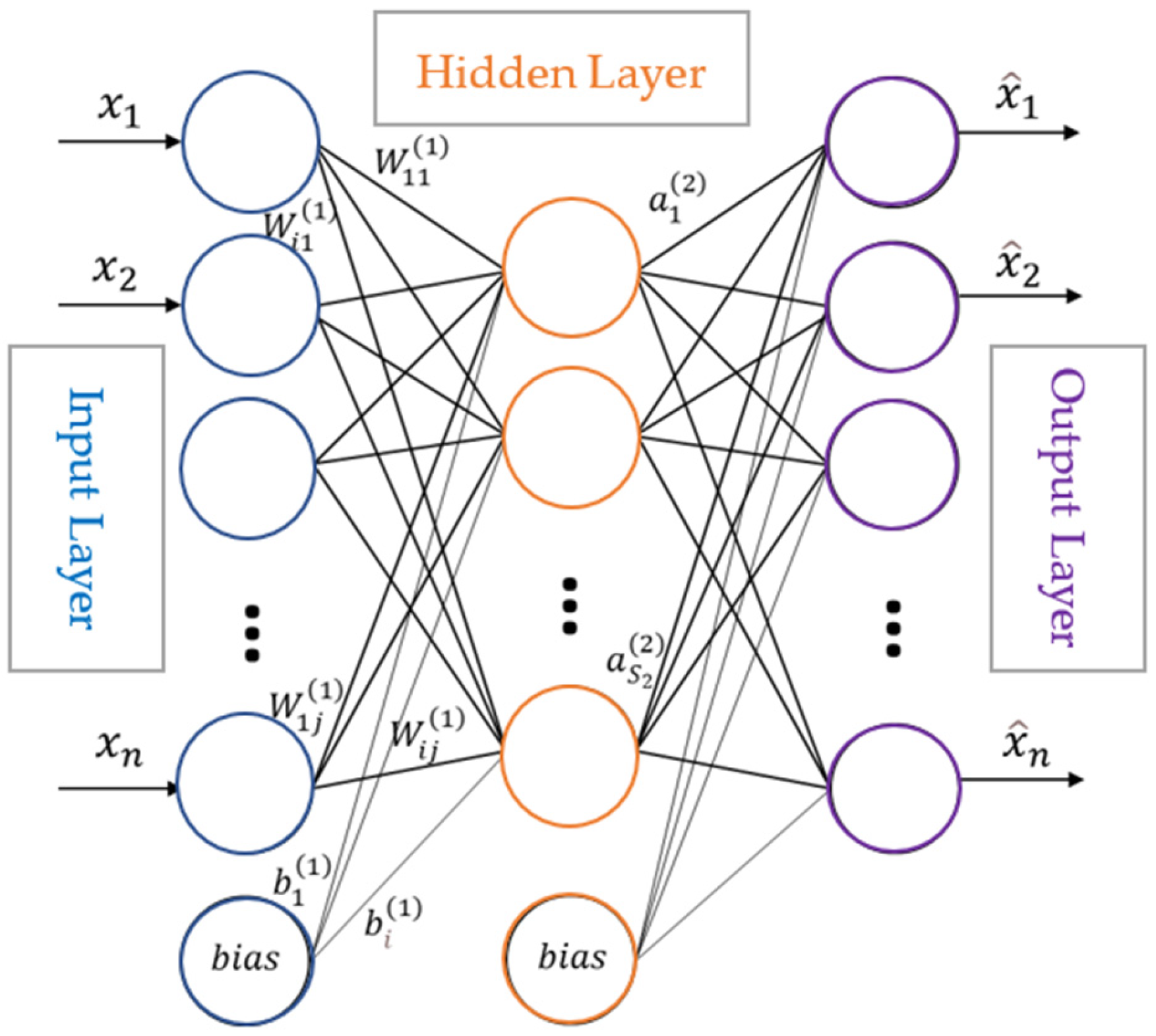
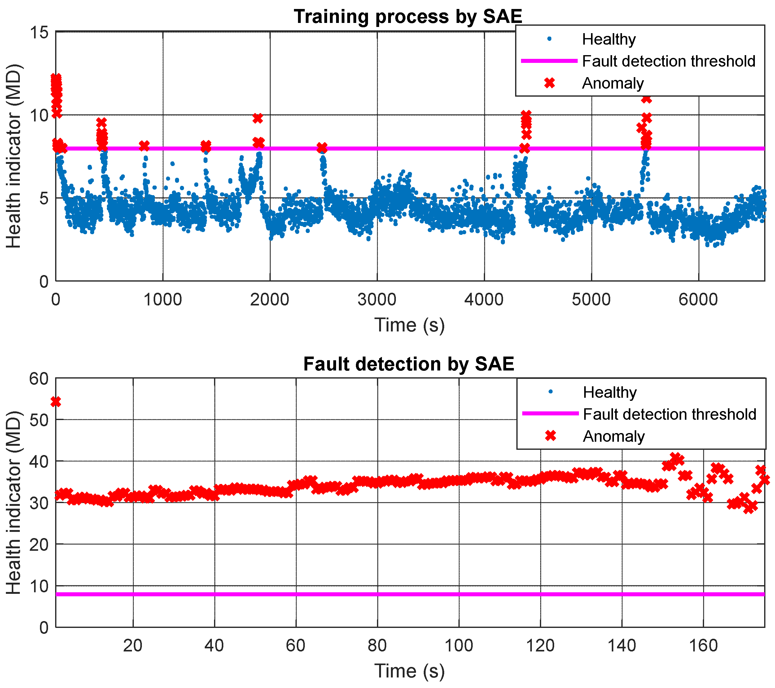
2.2. Sparse Autoencoder Model

The SAE [28] avoids directly copying the input from the input layer to the hidden layer, as often done in traditional autoencoders, and extracts the hidden distribution characteristics of data based on multi-layer nonlinear transformations. The sparse features are obtained by the sparse penalty term. Thus, the SAE is efficient and has more promising application possibilities. In fact, the SAE can be regarded as a special neural network with equal numbers of inputs and outputs, as shown in Figure 1. In the diagram, a circle indicates a neuron. The data transmitted by the input layer are encoded and reconstructed in the hidden layer, transforming the high-dimensional input into low-dimensional encoding characteristic vectors. Thus, there is an encoder connecting the input layer and hidden layer and a decoder linking the hidden layer and output layer. For an unlabeled sample set $\left\{x_1,x_2,\dots ,x_n\right\}$, the sigmoid function is chosen as the neuron activation function. Take a $n\times 1$ sample vector as the input, and define the i-th neuron activation amount $a_i^{\left(2\right)}$ as

$$a_i^{\left(2\right)}=f({\displaystyle \sum }_{j=1}^n{W}_{ij}^{\left(1\right)}{x}_j+b_i^{\left(1\right)}),$$

(6)

where $x_j$ is the j-th neuron value in the input layer, $W_{ij}^{\left(1\right)}$ represents the connection weight between the j-th neuron and the i-th neuron in the hidden layer, n is the number of neurons in the input layer, $b_i^{\left(1\right)}$ denotes the bias of the input layer i-th neuron, and f has the following expression:

$$f \left(z\right)=\frac{1}{1+e^{-z}}.$$

(7)

The hidden layer extracts the data features and the feature expression can minimize the errors in reconstructions. The feature expression in the hidden layer can be described as

$$h_{W,b}\left(x\right)=\left[\begin{array}{c}{a}_1^{\left(2\right)}\\ a_2^{\left(2\right)}\\ \dots \\ a_{S_2}^{\left(2\right)}\end{array}\right]=\left[\begin{array}{c}f({\displaystyle {\displaystyle \sum }_{j=1}^{S_1}}{W}_{1j}^{\left(1\right)}{x}_j+b_1^{\left(1\right)})\\ f({\displaystyle {\displaystyle \sum }_{j=1}^{S_1}}{W}_{2j}^{\left(1\right)}{x}_j+b_2^{\left(1\right)})\\ \dots \\ f({\displaystyle {\displaystyle \sum }_{j=1}^{S_1}}{W}_{S_{2}j}^{\left(1\right)}{x}_j+b_{S_2}^{\left(1\right)})\end{array}\right],$$

(8)

where $h_{W,b}\left(x\right)$ is the input layer feature matrix and $S_2$ is the number of neurons in the hidden layer. To minimize the reconstruction errors, a sparsity penalty function is introduced:

$$J_s \left(W,b\right)=\left[\frac{1}{m}{\displaystyle \sum }_{i=1}^m\frac{1}{2}\parallel h_{W,b}\left(x^{\left(i\right)}\right)-x^{\left(i\right)}\parallel { }^2\right]+\frac{\lambda }{2}{\displaystyle \sum }_{l=1}^{n-1}{\displaystyle \sum }_{i=1}^{S_l}{\displaystyle \sum }_{j=1}^{S_{l+1}}{(W_{ji}^{\left(l\right)})}^2+\beta {\displaystyle \sum }_{i=1}^{S_2}KL(\rho \parallel {\rho }_i).$$

(9)

where the first term $\frac{1}{m}{\displaystyle \sum }_{i=1}^m\frac{1}{2}\parallel h_{W,b}\left(x^{\left(i\right)}\right)-x^{\left(i\right)}\parallel { }^2$ denotes the mean squared error, and it is used to minimize the error between the input data and the output data. The second term $\frac{1}{2}{\displaystyle \sum }_{l=1}^{n-1}{\displaystyle \sum }_{i=1}^{S_l}{\displaystyle \sum }_{j=1}^{S_{l+1}}{(W_{ji}^{\left(l\right)})}^2$ represents the regularization and this term is used to avoid over-fitting. The last term ${\displaystyle \sum }_{i=1}^{S_2}KL(\rho \parallel {\rho }_i)$ in the equation is called sparsity regularization, and it imposes a sparsity constraint on the hidden units. $\lambda$ is the coefficient for the regularization term. $\beta$ is the coefficient for the sparsity regularization term. $KL(\rho \parallel {\rho }_i)$ measures the difference between two distributions, and this term can be given by the Kullback–Leibler divergence function.

2.3. Status Indicator for Machine Health

The Mahalanobis distance (MD) [29,30,31] synthesizes all the monitored variables and generates a threshold to determine the health status of the marine engine during the training process. It is a unitless measure with correlations between variables being included. Its advantage is that a single distance quantity is provided for multi-dimensional data sets. The Mahalanobis distance is calculated as

$$M{d}_i=\sqrt{\left(\left(Y_i-\widehat{Y_i}\right)-\overline{\mu }\right)S^{-1}{\left(\left(Y_i-\overline{Y_i}\right)-\overline{\mu }\right)}^T},$$

(10)

where $Y_i$ represents the i-th feature, $\widehat{Y_i}$ is a reconstruction of the feature, and $\overline{\mu }$ and S are the mean and covariance of the samples.

Next, the fault detection threshold $M{d}_{th}$ can be obtained from the probability density function (PDF) of $h$ for a given confidence level $\alpha$ by solving Equation (11):

$$P(h<d)={{\displaystyle \int }}_{-\infty }^{d}p\left(h\right)dh=\alpha ,$$

(11)

where $p\left(h\right)$ is the PDF function of $h$. The kernel density estimation (KDE) method is applied for distribution fitting. The KDE method is a well-established approach in statistical distribution fitting and has been successfully applied to the field of process monitoring and fault detection. According to the KDE method, $p\left(h\right)$ can be written as

$$\begin{array}{c}p\left(h\right)=\frac{1}{N\sigma }{\displaystyle {\displaystyle \sum }_{i=1}^N}K(\frac{h-h_i}{\sigma })\end{array},$$

(12)

where $N$ is the total number of $h$. $K\left(\cdot \right)$ is the kernel function and $\sigma$ is the bandwidth. The selection of the optimal value for $\sigma$ is described in [32]. Here, the Gaussian kernel [28] is used.

3. Physics-Based Multivariate Models

The physics-based models for monitored variables are linked with the working status of the marine engine. They rely on the inherent mechanism analysis of different faults to determine a group of dependent variables. Often, the grouped variables are key indicators of a specific fault. In general, the multivariate model for a monitored variable can be expressed by a least-term r-order surrogate function as

$$\begin{array}{cc}\hfill H\left(x_1,x_2,\cdots , x_k\right)& ={\phi }_{0,\dots ,0}+{\phi }_{1,0,\dots ,0}{x}_1+{\phi }_{0,1,0\dots ,0}{x}_2+\cdots +{\phi }_{0,\dots ,0,1}{x}_k,+{\phi }_{1,1,0,\dots ,0}{x}_1{x}_2+\cdots +{\phi }_{1,1,0,\dots ,0}{x}_m^2+\cdots \hfill \\ & +{\phi }_{r,0,\dots ,0}{x}_1^r+\cdots +{\phi }_{0,\dots ,0,r}{x}_k^r,\hfill \end{array}$$

(13)

where $x_1,x_2,\cdots , x_k$ are the variables used to build the model, and the number of variables is k; r represents the order of the surrogate model function; ${\phi }_{i_1,i_{2,}\cdots ,i_k}$ is the model coefficient, respectively. To reduce the computational effort, the number of terms in the model function is kept to the minimum, which is realized by setting $0\le i_1+i_2+\cdots +i_k\le r$.

The unknown model coefficient vector $\phi$ is determined by the nonlinear regression based on the least-square technique using the baseline data. When new data are collected, they will be evaluated via the surrogate function by comparing the predicted value with the measured one. Taking a variable p as an example, this process can be described by

$$\widehat{p}=H_p\left({\tilde{x}}_1,{\tilde{x}}_2,\cdots ,{\tilde{x}}_k\right),$$

(14)

$$Re\left(p\right)=\tilde{p}-\widehat{p},$$

(15)

where $H_p$ represents the multivariate model for variable p, $\widetilde{·}$ denotes the measured value, and $\widehat{·}$ denotes the predicted value, respectively. Re (p) is the residual between the model prediction and measurement for variable p. The fault threshold, ${\gamma }_p$, is generated in the prediction step by the confidence interval measure. Thus, the health status of the variable can be determined by

$$Re\left(p\right)=\tilde{p}-\widehat{p},$$

(16)

To avoid false alarms, a variable is diagnosed as abnormal when consecutive data points fall outside of the predicted confidence interval or the residual exceeds the permitted limits.

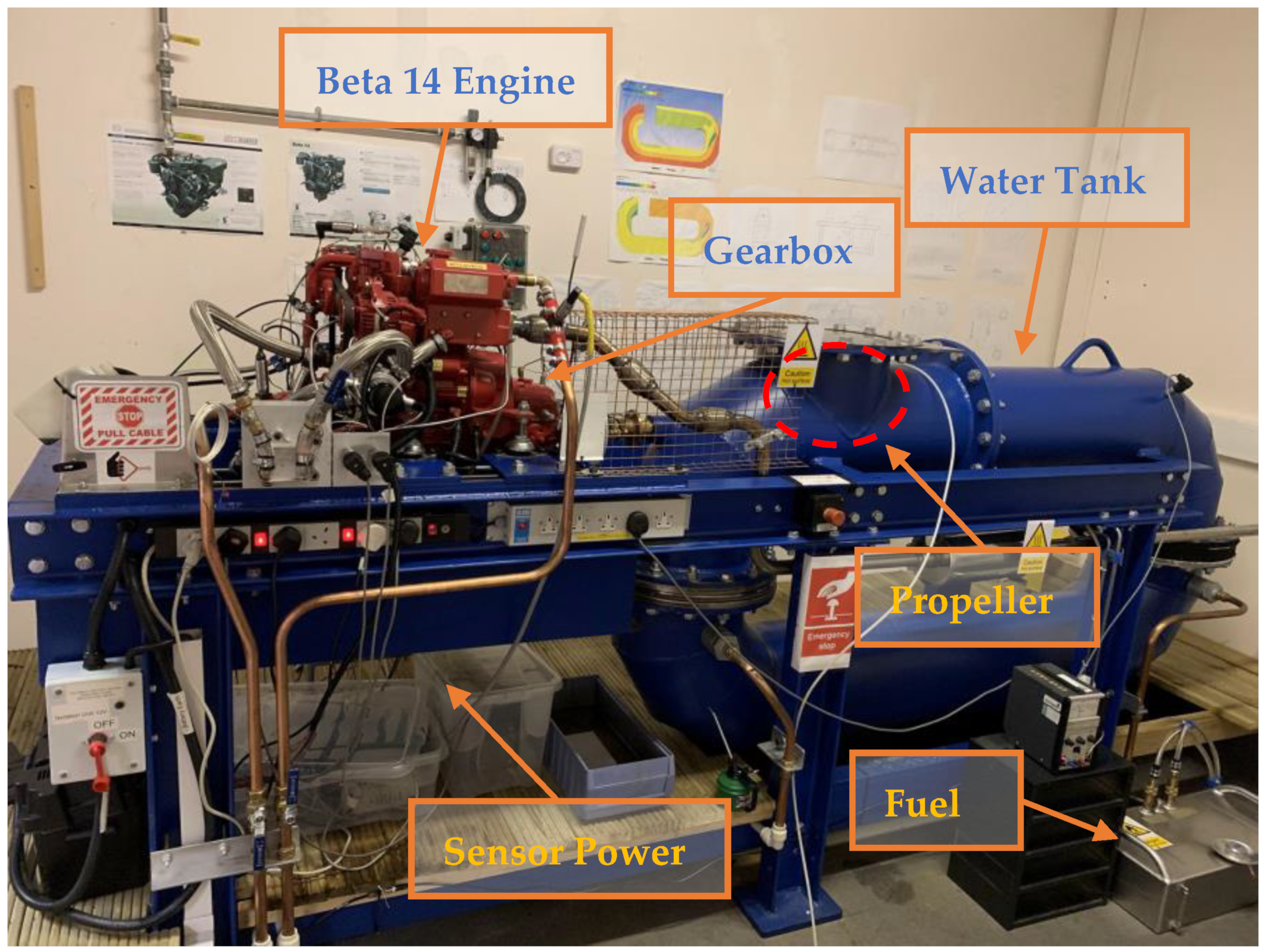
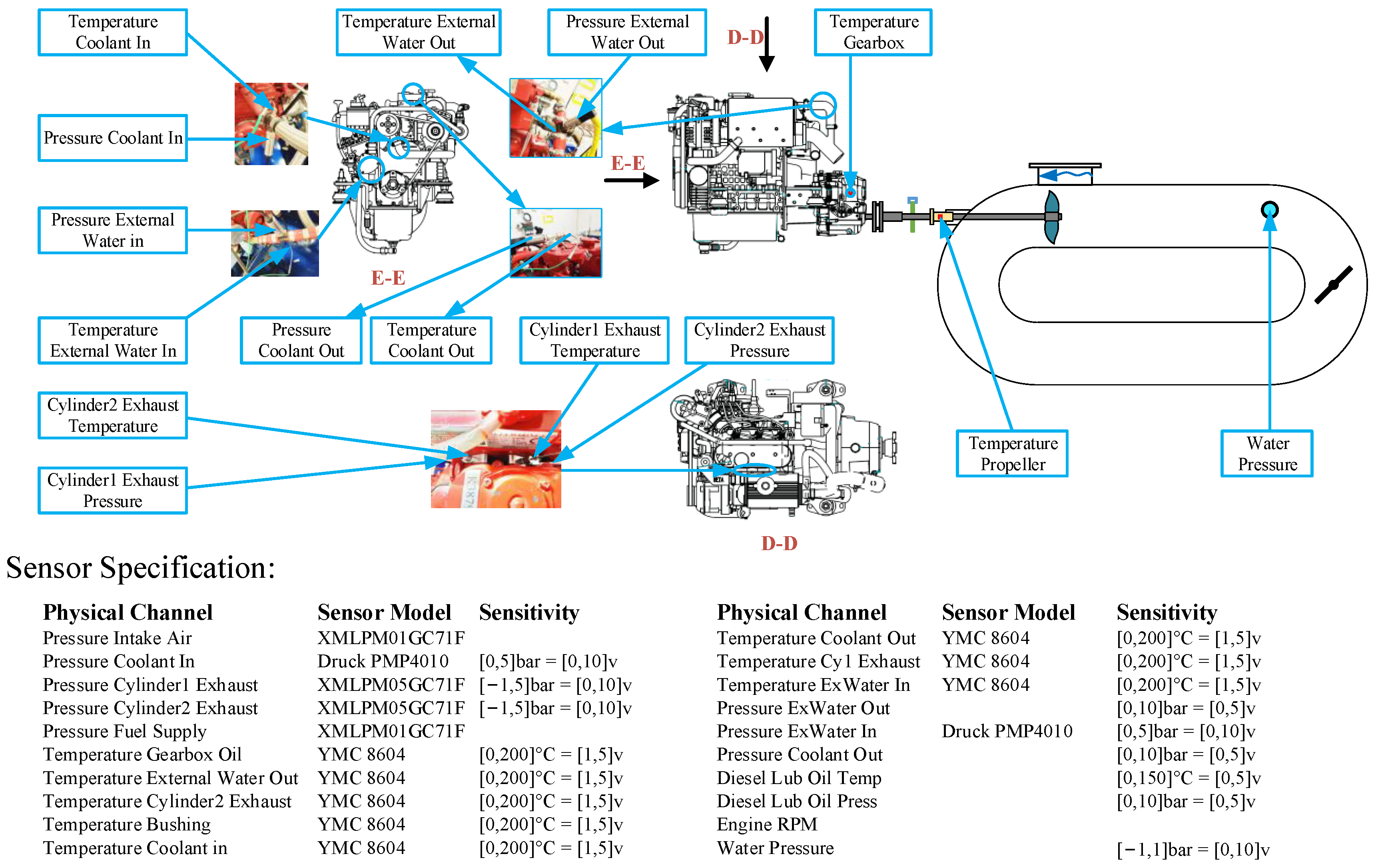
4. Marine Engine Test Rig

A marine engine test rig is set up, as demonstrated in Figure 2. The marine power system has a Beta 14 diesel engine, a gearbox, and a propeller immersed in water. It can be used to simulate many typical faults in a marine power system. The temperatures and pressures of the internal and external coolants at the inlet and outlet, lubrication systems, and gearbox are measured. The average rotating speed of the engine is calculated by the engine parameters and flywheel instantaneous angular speed. The water pressure in the water tank is recorded as an indicator of the load level, which is adjusted by a valve on the tank. Thus, the load level on the propeller and the rotating speed of the engine can be used to reflect the key working condition parameters. A complete list of monitored process data and the descriptions are provided in

Table 1. Variables monitored in the test rig.

No.	Short Form	Detail
1	Pressure Intake Air	Intake air pressure of engine
2	Pressure Coolant In	Internal coolant water pressure at inlet
3	Pressure Coolant Out	Internal coolant water pressure at outlet
4	Pressure Cy1 Exhaust	Exhaust air pressure of cylinder 1
5	Pressure Cy2 Exhaust	Exhaust air pressure of cylinder 2
6	Pressure Fuel Supply	Pressure of fuel supply to engine
7	Pressure Ex Water In	External coolant water pressure at inlet
8	Pressure Ex Water Out	External coolant water pressure at outlet
9	Pressure Lub Oil	Lube oil pressure
10	Pressure Water Tank	Water pressure in water tank/load level
11	Engine Speed RPM	Averaged rotating speed of shaft
12	Temperature Gearbox	Gearbox housing temperature
13	Temperature Bushing	Journal bearing (before propeller) oil temperature
14	Temperature Coolant in	Internal coolant water temperature at inlet
15	Temperature Coolant Out	Internal coolant water temperature at outlet
16	Temperature Cy1 Exhaust	Exhaust air temperature of cylinder 1
17	Temperature Cy2 Exhaust	Exhaust air temperature of cylinder 2
18	Temperature Ex Water In	External coolant water temperature at inlet
19	Temperature Ex Water Out	External coolant water temperature at outlet
20	Temperature Lub Oil	Lube oil temperature

. The sensor placement and sensor models with their sensitivities are exhibited in Figure 3. These data can satisfy the requirements in observing the running status and health condition of the marine power system. The acquisition rate for data collection is 1 Hz, i.e., there is one data point for each variable per second. The experimental tests are completed by using in-house software, including main modules such as the data connection, history analysis and visualization, measurement parameter setting, and further data processing. Data processing for the results in this study is implemented in Matlab. Baseline testing is conducted for many combinations of rotating speeds and load levels to enable sufficient training of the models. In the present study, the lubrication filter blockage and cylinder leakage faults in the marine engine are investigated based on the previously described methods.

5. Case Studies

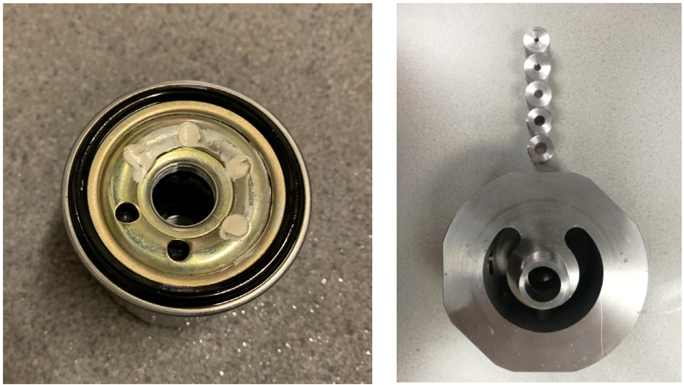
5.1. Filter Blockage

The lubrication oil filter keeps the oil clean and ensures the lubrication performance to extend the life of critical friction pairs. In practice, external elements, such as water, dust and particles, and oil oxide, will cause the blocking of the filters. When a filter blockage fault happens, insufficient lubrication oil is circulated into the engine, decreasing the performance of the marine engine. A direct consequence of filter blocking is a drop in the lubrication oil pressure. Two strategies are used to simulate this fault on the marine engine test rig. As can be seen in Figure 4, a circular device is designed to guide the oil flow and provide space to control the oil volume. The oil will circulate from the cooler into the circular passage and then enters the engine from the central hole. On the one hand, the circular holes on the cover are partially blocked manually. On the other hand, the hole size at the center is adjusted and reduced by additional bolts. The oil pressure is measured after the clog and the tests are conducted at around 1300 RPM.

Figure 5 shows the fault detection results using the PCA- and SAE-based methods when the machine runs under healthy conditions. As can be seen, the fault detection models believe that the machine works normally, because almost all the points are below the thresholds. The training process using the baseline data by PCA (upper figure) and the fault diagnosis process (lower figure) using the fault simulation test data are shown in Figure 6. A fault threshold is generated in the training process and data points with an MD index higher than the threshold are deemed abnormal. It is observed that 99% of the data collected in the health status are treated as normal, while the remaining 1% are treated as abnormal, bearing in mind that there still can be extreme points and uncertainty during normal conditions. Figure 6 suggests that the diagnosis process has successfully identified anomalies when the filter blockage fault happens, evidenced by the fact that all fault data points are above the threshold line. The Q-statistic method is employed to inspect the contributions of variables in the detection process and the contribution map is plotted in Figure 7. Furthermore, the residual map of all variables is plotted in Figure 8, in which the sign of the residual of a variable indicates whether the variable is higher or lower than normal. It can be noticed from Figure 7 that the first three major contributors in the PCA model for the diagnosis of the filter blockage fault are the external coolant water pressure at the outlet, the averaged engine rotating speed, and the internal coolant water temperature. Figure 8 shows that the residual for the lubrication oil pressure is positive, suggesting that the measured values are higher than the predicted values. It can be concluded that the PCA model has detected the filter blockage fault and can inform users that the marine engine is abnormal. However, neither the contribution map nor the residual map provides the correct classification of variable evolutions. In other words, the PCA model can detect novelties but is incapable of isolating the filter blockage fault.

The training and detection process for the filter blockage fault using the SAE model is demonstrated in Figure 9. The MD indices for fault data points are obviously higher than the threshold in the SAE model, showing that the SAE method detects the abnormality in the marine engine system. On this point, the SAE has a similar ability to PCA. The contribution map and residual map of the SAE model for the filter blockage fault are given in Figure 10 and Figure 11. From Figure 11, it is found that the residual for the lubrication oil pressure is negative, meaning that the measured data are lower than the predicted value, which is consistent with reality and proves that the SAE outperforms the PCA in this regard. However, as can be seen from Figure 10, the lubrication oil pressure does not appear either in the first three major contributors in the SAE model, which are the external coolant water pressure at the inlet, the internal coolant water temperature at the inlet, and the exhaust air temperature of the cylinders. Thus, the SAE model is able to detect the filter blockage and reveals the drop in the lubrication oil pressure. However, it cannot accurately isolate the filter blockage fault in the marine engine. The above results reflect a common issue in data-driven models, i.e., poor interpretability. These methods use pure data sets and explore their patterns, and do not rely on the physics of the marine engine, which leads to contribution analysis results that are unreasonable.

In physics-based modeling, the average rotating speed and load level are used as working condition parameters, i.e., other variables are deemed to be dependent on these two parameters. In this regard, all the monitored variables have their own models. Similarly, the baseline data are used to train the models and the data collected for fault simulation tests are then evaluated by the models to check whether any novelty occurs. For the filter blockage fault, the lubrication oil pressure is the most important quantity. The training and diagnosis process based on its physics-based model is plotted in Figure 12, where dashed lines in different colors indicate the model’s predicted 99% confidence intervals, while solid lines plot the measured data. It is observed from the results that the measured lubrication oil pressure is below 2.5 bar, while the predicted band is around 3.2–3.7 bar. The values are significantly lower than the predicted confidence interval, suggesting the fault status of the marine engine. Other monitored variables fall within their respective confidence intervals, indicating that they are healthy. For brevity, the results are not presented here. From the above analysis, it can be found that the physics-based monitoring involves mechanism inference before the diagnosis and the filter blockage fault is successfully isolated. Moreover, the evolution characteristics agree with the principles of the marine engine. Compared with the PCA and SAE models, the physics-based models are more accurate in isolating fault types as they all identified the anomalies.

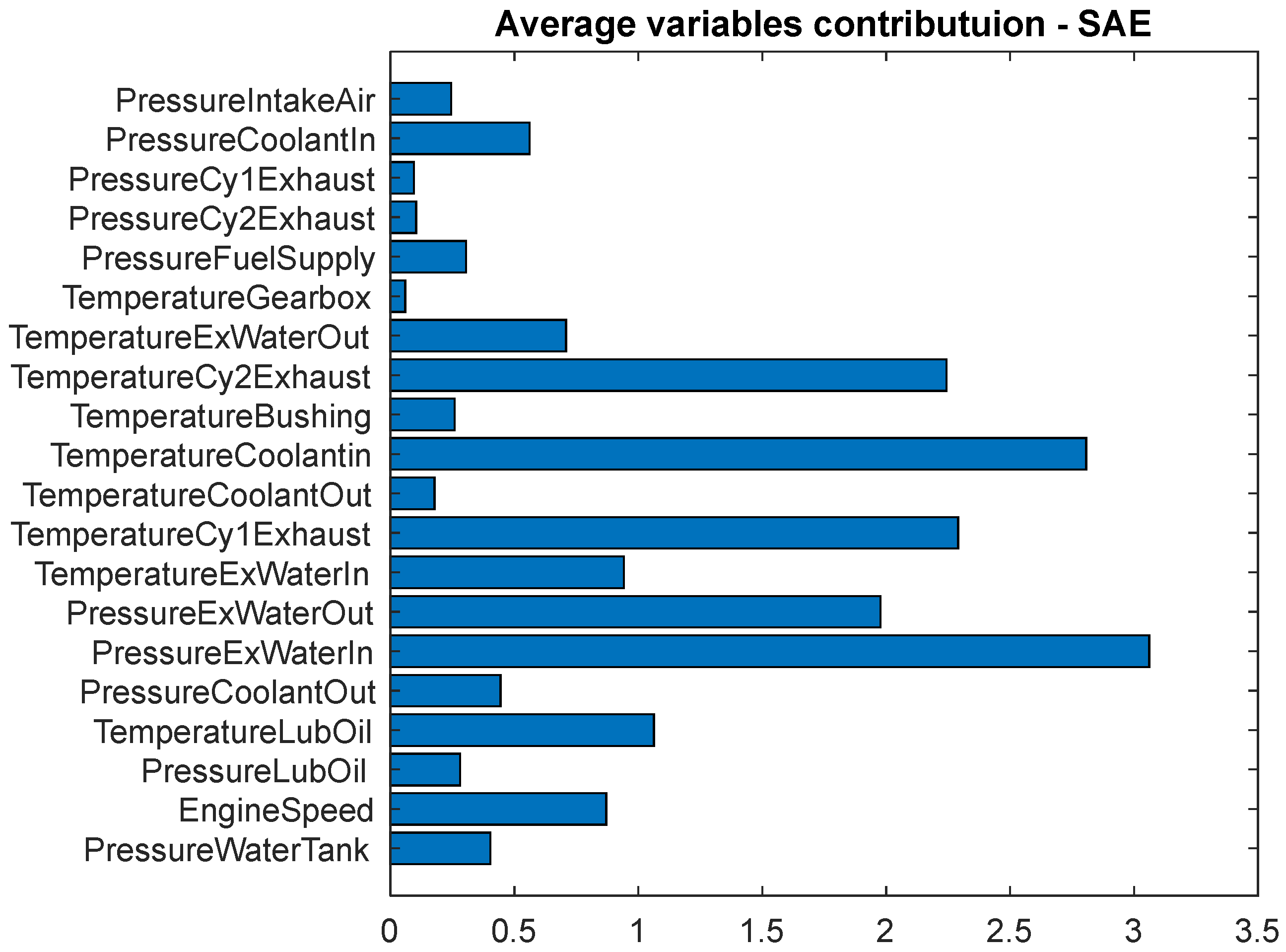
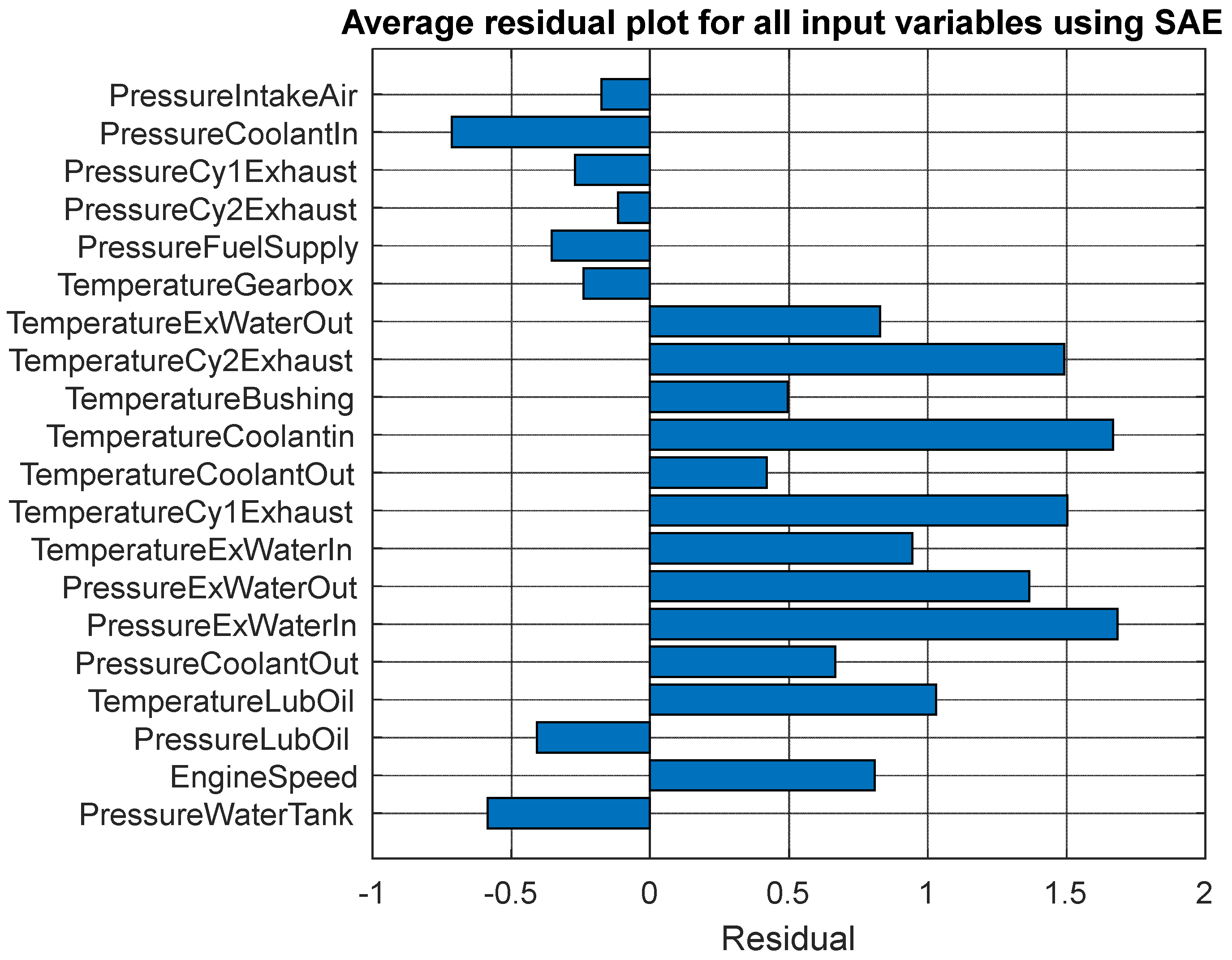
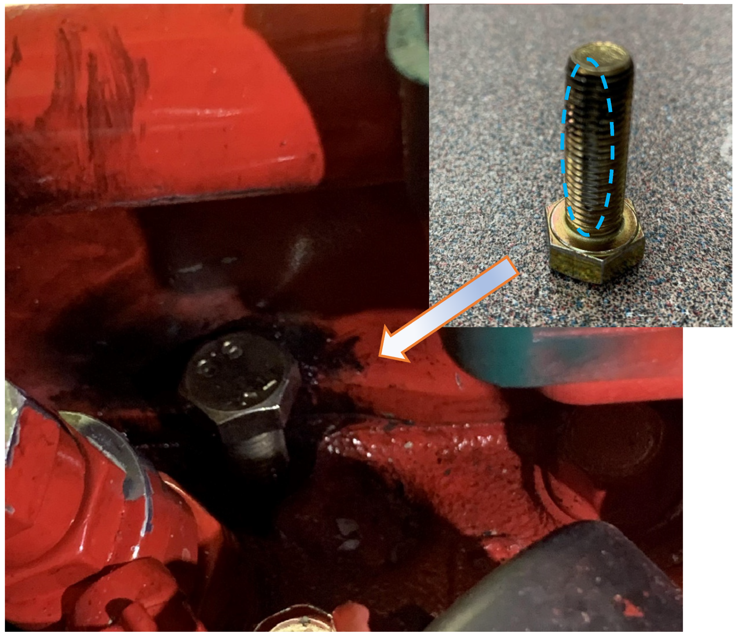
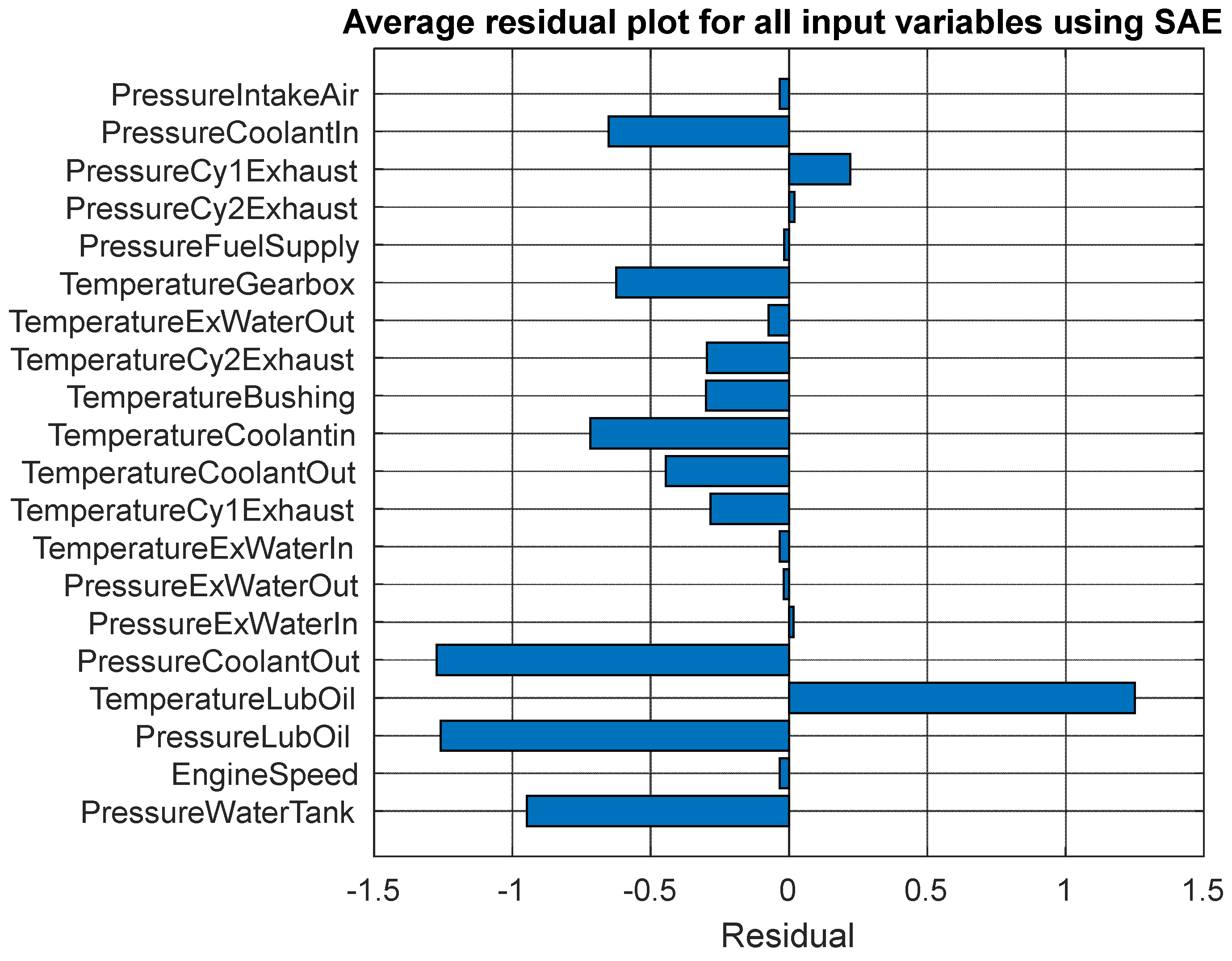
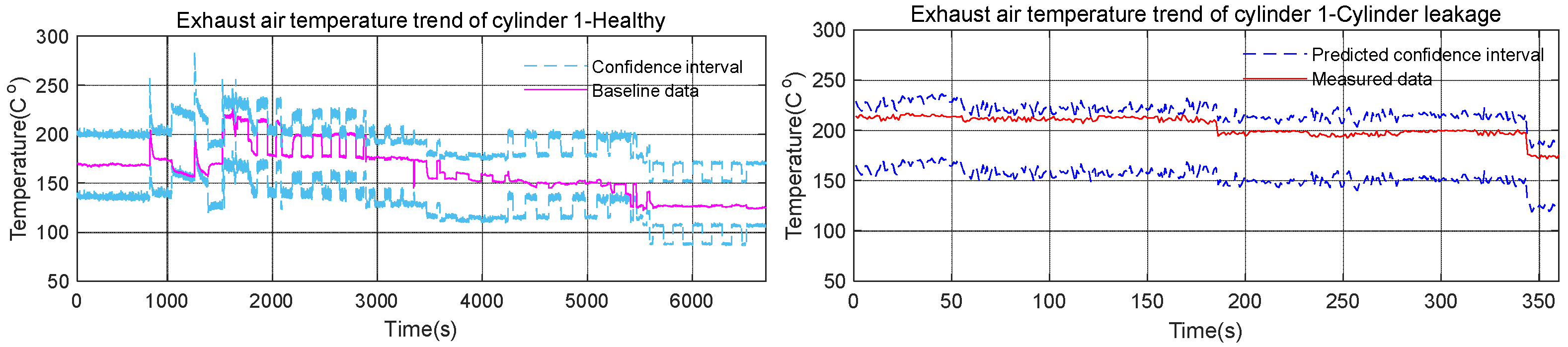
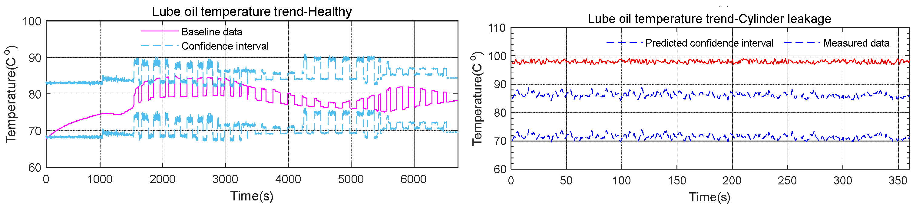
5.2. Cylinder Leakage

The cylinder leakage fault refers to the leakage of gas in the cylinder and can be caused by the loosening of the valve and fuel injector seal, wear of the piston ring, cylinder liner and piston wear, and cylinder pad damage. It will affect the power generated by the engine and the lubrication oil consumption and produce more harmful particles. To simulate the cylinder leakage fault, grooved bolts are designed to allow leakage from the cylinders. The specimen is then installed to replace the original bolt in cylinder 2, as shown in Figure 13. The test for fault conditions is carried out for the marine engine under a rotating speed of around 1600 rpm. The same data sets are used for the data-driven models and physics-based models for fault detection and isolation.

The training and fault diagnosis process for the cylinder leakage fault based on the PCA model is given in Figure 14. The same strategy as in the previous subsection, where 1% of the healthy data are deemed abnormal, is used for the training. Any red cross markers suggest a fault data point. All the points above the threshold line are diagnosed as faulty. It can be noticed that the fault status of the marine engine with the cylinder leakage fault is secured by the PCA model, evidenced by the data points being higher than the threshold. Figure 15 and Figure 16 plot the contribution map and residual map for monitored variables based on the Q-statistic method. It is found that the identified first three variables that contribute to the detection are the lubrication oil temperature, the internal coolant water pressure at the inlet, and the gearbox temperature. The results are unreasonable according to the physics of the marine engine, except for the first contributor. The residual of the leaked cylinder exhaust air temperature is negative, indicating that its measured values are lower than normal values. This is natural due to the fault implemented. The residual of the lubrication oil temperature is negative as well. However, this result does not agree with the fault mechanism of the cylinder leakage. Therefore, the PCA model again can only detect the fault status of the system, while it cannot isolate the cylinder leakage fault.

Based on the SAE model, the training and fault detection results are plotted in Figure 17. Again, it is evident that the malfunctions of the marine engine are identified since all the measured data points exceed the fault threshold line. To further clarify the contributions of variables in the model, the contribution map and residual map are shown in Figure 18 and Figure 19. Apparently, the order of major contributors in detecting anomalies is the interval coolant water pressure, the lubrication oil pressure, and the lubrication oil temperature. The residual of the leaked cylinder exhaust air temperature is negative and that of the lubrication oil temperature is positive. Therefore, the leaked cylinder exhaust air temperature drops from the predicted value and the lubrication oil temperature is increased, which is consistent with the physical principles of the marine engine. Thus, it is safe to conclude that the SAE model has successfully detected the fault and sorted out the variable evolutions correctly. However, the variable contribution of the leaked cylinder exhaust air temperature is not the largest, causing difficulties in isolating the fault type. From the above discussion, it is clear that the SAE and PCA can both report abnormalities of the marine engine regarding the cylinder leakage fault. The SAE predicts more accurate variable contributions than the PCA, while both of them fail to predict the fault type.

The training and diagnosis process based on the physics-based model is exhibited in Figure 20, Figure 21 and Figure 22. It can be observed that the exhaust air temperature of the leaked cylinder falls below the predicted 99% confidence interval significantly, reflecting the malfunctions in cylinder 2’s combustion. On the contrary, the exhaust air temperature of cylinder 1 is normal as the measured data are within the confidence interval. Moreover, the lubrication oil temperature is higher than the predicted range. These results agree with the fault mechanism of the cylinder leakage. Thus, the physics-based model can detect and isolate the cylinder leakage fault, as well as identify the fault location. From this point of view, the physics-based model is superior in isolating faults compared with the data-driven models, which can produce results with poor interpretability. The physics-based models are not intelligent or convenient enough compared with the data-driven models in terms of transferability, i.e., the physics-based models vary between engines.

6. Conclusions

In the present work, comparative studies on the condition monitoring and fault detection of a marine engine are carried out based on unsupervised data-driven models and physics-based models. The lubrication oil filter blockage and cylinder leakage faults are investigated regarding the performance of both types of models. It is found from the results that the two categories of models can effectively detect abnormalities in the marine engine. The data-driven models classify the data points for faults to be 2–4 times higher than the thresholds. The physics-based model shows a sharp drop in the lubrication oil pressure from a confidence interval with a lower limit larger than 3 to 2.3 bar in the filter blockage fault, and a decrease of about 50 °C in the leaked cylinder exhaust gas temperature is detected in simulating the cylinder leakage fault. In the latter, the lubrication oil temperature also shows a value about 20 °C higher than the predicted upper limit of the 99% confidence interval. The sparse autoencoder model predicts more accurate critical variable residual maps than the principal component analysis. However, they cannot identify the most significant contributors to faults and fail to isolate the faults. The physics-based model works well in detecting novelty and isolating faults. It can be concluded that the unsupervised data-driven models have excellent transferability, while they are prone to generating some results that have poor interpretability because they rely solely on data sets and are independent of the physics of the marine engine. On the other hand, the physics-based model shows results that are easy to interpret, but they are not transferable among different systems. The results and discussion in this paper provide a reference for the condition monitoring of marine engines and future directions for more accurate fault detection.

References

1. Castresana, J.; Gabiña, G.; Martin, L.; Basterretxea, A.; Uriondo, Z. Marine diesel engine ANN modelling with multiple output for complete engine performance map. Fuel 2022, 319, 123873. [Google Scholar] [CrossRef]
2. Ou, S.; Yu, Y.; Yang, J. Identification and reconstruction of anomalous sensing data for combustion analysis of marine diesel engines. Measurement 2022, 193, 110960. [Google Scholar] [CrossRef]
3. Liu, L.; Chen, X.; Liu, D.; Du, J.; Li, W. Combustion phase identification for closed-loop combustion control by resonance excitation in marine diesel engines. Mech. Syst. Signal Process. 2022, 163, 108115. [Google Scholar] [CrossRef]
4. Fog, T.L.; Hansen, L.K.; Larsen, J.; Hansen, H.; Madsen, L.; Sorensen, P.; Hansen, E.; Pedersen, P. On condition monitoring of exhaust valves in marine diesel engines. In Proceedings of the Neural Networks for Signal Processing IX: Proceedings of the 1999 IEEE Signal Processing Society Workshop, Madison, WI, USA, 25 August 1999; pp. 554–563. [Google Scholar]
5. Sun, L.; Ren, X.; Zhou, H.; Li, G.; Yang, W.; Zhao, J.; Liu, Y. Machining Quality Prediction of Marine Diesel Engine Block Based on Error Transmission Network. Machines 2022, 10, 1081. [Google Scholar] [CrossRef]
6. Sakellaridis, N.F.; Raptotasios, S.I.; Antonopoulos, A.K.; Mavropoulos, G.C.; Hountalas, D.T. Development and validation of a new turbocharger simulation methodology for marine two stroke diesel engine modelling and diagnostic applications. Energy 2015, 91, 952–966. [Google Scholar] [CrossRef]
7. Chen, K.; Mao, Z.; Zhao, H.; Jiang, Z.; Zhang, J. A Variational Stacked Autoencoder with Harmony Search Optimizer for Valve Train Fault Diagnosis of Diesel Engine. Sensors 2020, 20, 223. [Google Scholar] [CrossRef]
8. Han, P.; Ellefsen, A.L.; Li, G.; Holmeset, F.T.; Zhang, H. Fault Detection With LSTM-Based Variational Autoencoder for Maritime Components. IEEE Sens. J. 2021, 21, 21903–21912. [Google Scholar] [CrossRef]
9. Bai, H.; Zhan, X.; Yan, H.; Wen, L.; Yan, Y.; Jia, X. Research on Diesel Engine Fault Diagnosis Method Based on Stacked Sparse Autoencoder and Support Vector Machine. Electronics 2022, 11, 2249. [Google Scholar] [CrossRef]
10. Yan, X.; Sheng, C.; Zhao, J.; Yang, K.; Li, Z. Study of on-line condition monitoring and fault feature extraction for marine diesel engines based on tribological information. Proc. Inst. Mech. Eng. Part O J. Risk Reliab. 2014, 229, 291–300. [Google Scholar] [CrossRef]
11. Wang, J.; Sun, X.; Zhang, C.; Ma, X. An integrated methodology for system-level early fault detection and isolation. Expert Syst. Appl. 2022, 201, 117080. [Google Scholar] [CrossRef]
12. Fu, C.; Sinou, J.-J.; Zhu, W.; Lu, K.; Yang, Y. A state-of-the-art review on uncertainty analysis of rotor systems. Mech. Syst. Signal Process. 2023, 183, 109619. [Google Scholar] [CrossRef]
13. Lynch, C.; Hagras, H.; Callaghan, V. Using Uncertainty Bounds in the Design of an Embedded Real-Time Type-2 Neuro-Fuzzy Speed Controller for Marine Diesel Engines. In Proceedings of the 2006 IEEE International Conference on Fuzzy Systems, Vancouver, BC, Canada, 16–21 July 2006; pp. 1446–1453. [Google Scholar]
14. Fu, C.; Ren, X.; Yang, Y. Vibration Analysis of Rotors Under Uncertainty Based on Legendre Series. J. Vib. Eng. Technol. 2019, 7, 43–51. [Google Scholar] [CrossRef]
15. Wang, R.; Chen, H.; Guan, C. A Bayesian inference-based approach for performance prognostics towards uncertainty quantification and its applications on the marine diesel engine. ISA Trans. 2021, 118, 159–173. [Google Scholar] [CrossRef] [PubMed]
16. Zhang, P.; Gao, Z.; Cao, L.; Dong, F.; Zou, Y.; Wang, K.; Zhang, Y.; Sun, P. Marine Systems and Equipment Prognostics and Health Management: A Systematic Review from Health Condition Monitoring to Maintenance Strategy. Machines 2022, 10, 72. [Google Scholar] [CrossRef]
17. Wang, X.; Cai, Y.; Li, A.; Zhang, W.; Yue, Y.; Ming, A. Intelligent fault diagnosis of diesel engine via adaptive VMD-Rihaczek distribution and graph regularized bi-directional NMF. Measurement 2021, 172, 108823. [Google Scholar] [CrossRef]
18. Xi, W.; Li, Z.; Tian, Z.; Duan, Z. A feature extraction and visualization method for fault detection of marine diesel engines. Measurement 2018, 116, 429–437. [Google Scholar] [CrossRef]
19. Liu, Y.; Gan, H.; Cong, Y.; Hu, G. Research on fault prediction of marine diesel engine based on attention-LSTM. Proc. Inst. Mech. Eng. Part M J. Eng. Marit. Environ. 2022, 237, 508–519. [Google Scholar] [CrossRef]
20. Hou, L.; Zhang, J.; Du, B. A fault diagnosis model of marine diesel engine fuel oil supply system using PCA and optimized SVM. In Journal of Physics: Conference Series, Proceedings of the 4th International Conference on Artificial Intelligence, Automation and Control Technologies (AIACT 2020), Hangzhou, China, 24–26 April 2020; IOP Publishing Ltd.: Bristol, UK, 2020; p. 012045. [Google Scholar]
21. Wang, X.; Kruger, U.; Irwin, G.W.; McCullough, G.; McDowell, N. Nonlinear PCA with the local approach for diesel engine fault detection and diagnosis. IEEE Trans. Control Syst. Technol. 2007, 16, 122–129. [Google Scholar] [CrossRef]
22. Zhong, K.; Li, J.; Wang, J.; Han, M. Fault Detection for Marine Diesel Engine Using Semi-supervised Principal Component Analysis. In Proceedings of the 2019 9th International Conference on Information Science and Technology (ICIST), Hulunbuir, China, 2–5 August 2019; pp. 146–151. [Google Scholar]
23. Wang, S.; Wang, J.; Ding, X. An Intelligent Fault Diagnosis Scheme Based On PCA-BP Neural Network for the Marine Diesel Engine. IOP Conf. Ser. Mater. Sci. Eng. 2020, 782, 032079. [Google Scholar] [CrossRef]
24. Zhang, D.; Wang, K.; Gao, J.; Che, X. Autoencoder and Deep Neural Network based Energy Consumption Analysis of Marine Diesel Engine. In Proceedings of the 2022 IEEE International Conference on Mechatronics and Automation (ICMA), Guilin, China, 7–10 August 2022; pp. 1692–1696. [Google Scholar]
25. Qu, C.; Zhou, Z.; Liu, Z.; Jia, S. Predictive anomaly detection for marine diesel engine based on echo state network and autoencoder. Energy Rep. 2022, 8, 998–1003. [Google Scholar] [CrossRef]
26. Velasco-Gallego, C.; Lazakis, I. Analysis of variational autoencoders for imputing missing values from sensor data of marine systems. J. Ship Res. 2022, 66, 193–203. [Google Scholar] [CrossRef]
27. Abdi, H.; Williams, L. Principal Component Analysis. Wiley Interdiscip. Rev. Comput. Stat. 2010, 2, 433–459. [Google Scholar] [CrossRef]
28. Liang, X.; Duan, F.; Bennett, I.; Mba, D. A Sparse Autoencoder-Based Unsupervised Scheme for Pump Fault Detection and Isolation. Appl. Sci. 2020, 10, 6789. [Google Scholar] [CrossRef]
29. De Maesschalck, R.; Jouan-Rimbaud, D.; Massart, D.L. The Mahalanobis distance. Chemom. Intell. Lab. Syst. 2000, 50, 1–18. [Google Scholar] [CrossRef]
30. Ghorbani, H. Mahalanobis distance and its application for detecting multivariate outliers. Facta Univ. Ser. Math. Inform. 2019, 3, 583–595. [Google Scholar] [CrossRef]
31. Sarmadi, H.; Entezami, A.; Saeedi Razavi, B.; Yuen, K.V. Ensemble learning-based structural health monitoring by Mahalanobis distance metrics. Struct. Control Health Monit. 2021, 28, e2663. [Google Scholar] [CrossRef]
32. Odiowei, P.E.P.; Cao, Y. Nonlinear Dynamic Process Monitoring Using Canonical Variate Analysis and Kernel Density Estimations. IEEE Trans. Ind. Inform. 2010, 6, 36–45. [Google Scholar] [CrossRef]
Figure 1. Structure of the sparse autoencoder.
Machines 11 00557 g001
Figure 2. Marine engine test rig.
Machines 11 00557 g002
Figure 3. Monitored variables in the marine system.
Machines 11 00557 g003
Figure 4. Filter blockage simulation.
Machines 11 00557 g004aMachines 11 00557 g004b
Figure 5. Anomaly detection results when the machine runs under healthy conditions based on the PCA and SAE methods.
Machines 11 00557 g005aMachines 11 00557 g005b
Figure 6. Training and anomaly detection process for filter blockage based on the PCA.
Machines 11 00557 g006
Figure 7. Contribution map for filter blockage fault based on the PCA.
Machines 11 00557 g007
Figure 8. Residual map for filter blockage fault based on the PCA.
Machines 11 00557 g008
Figure 9. Training and anomaly detection process for filter blockage based on the SAE.
Machines 11 00557 g009
Figure 10. Contribution map for filter blockage fault based on the SAE.
Machines 11 00557 g010
Figure 11. Residual map for filter blockage fault based on the SAE.
Machines 11 00557 g011
Figure 12. Training and anomaly detection process for filter blockage using the physics-based model: dashed lines—predicted 99% confidence intervals; solid lines—measured data.
Machines 11 00557 g012
Figure 13. Cylinder leakage simulation.
Machines 11 00557 g013
Figure 14. Training and anomaly detection process for cylinder leakage fault based on the PCA.
Machines 11 00557 g014
Figure 15. Contribution map for cylinder leakage fault based on the PCA.
Machines 11 00557 g015
Figure 16. Residual map for cylinder leakage fault based on the PCA.
Machines 11 00557 g016
Figure 17. Training and anomaly detection process for cylinder leakage fault based on the SAE.
Machines 11 00557 g017
Figure 18. Contribution map for cylinder leakage fault based on the SAE.
Machines 11 00557 g018
Figure 19. Residual map for cylinder leakage fault based on the SAE.
Machines 11 00557 g019
Figure 20. Training and anomaly detection process for cylinder leakage fault using the physics-based model for exhaust gas temperature of cylinder 1.
Machines 11 00557 g020
Figure 21. Training and anomaly detection process for cylinder leakage fault using the physics-based model for exhaust gas temperature of cylinder 2.
Machines 11 00557 g021
Figure 22. Training and anomaly detection process for cylinder leakage fault using the physics-based model for lubrication oil temperature.
Machines 11 00557 g022