Evaluation of Different Fault Diagnosis Methods and Their Applications in Vehicle Systems

Abstract

A high level of automation in vehicles is accompanied by a variety of sensors and actuators, whose malfunctions must be dealt with caution because they might cause serious driving safety hazards. Therefore, a robust and highly accurate fault detection and diagnosis system to monitor the operational states of vehicle systems is an indispensable prerequisite. In the area of fault diagnosis, numerous techniques have been studied, and each one has pros and cons. Selecting the best approach based on the requirements or usage scenarios will save much needless work. In this article, the authors examine some of the most common fault diagnosis methods for their applicability to automated vehicle systems: the traditional binary logic method, the fuzzy logic method, the fuzzy neural method, and two neural network methods (the feedforward neural network and the convolutional neural network). For each approach, the diagnosis algorithms for vehicle systems were modeled differently. The analysis of the detection capabilities and the suitable application scenarios of each fault diagnosis approach for vehicle systems, as well as recommendations for selecting different methods for various diagnosis needs, are also provided. In the future, this can serve as an effective guide for the selection of a suitable fault diagnosis approach based on the application scenarios for vehicle systems.

1. Introduction

To attain a high level of autonomous driving, sensors and actuators must work in concert with one another. Regardless of how advanced the sensors and actuators are, failures are always inescapable. Improving the dependability of sensors and actuators with a sensitive and stable fault monitoring system is always an effective solution. Fault detection is the process of determining whether a monitored system is defective. The next step following problem detection is fault diagnosis, which aims to determine the type of defect and, as exactly as possible, define its size, position, and detection time [1].

Fault diagnosis can be performed in several ways, such as with neural networks, fuzzy logic, evolutionary algorithms, support vector machines, etc. [2]. Diagnostic reasoning methods and classification methods are the two most common types. The diagnostic reasoning methods can also be realized as an expert knowledge-based approach. Expert knowledge is frequently stated in conventional expert systems as deterministic “IF-THEN“ rules, which are also the origin of the traditional binary logic fault diagnosis approach. Reference [3] utilized the expert system to diagnose the problem with the boiling water reactor and an onboard application for a brushless DC motor-driven actuator introduced in [4]. Instead of a simple fault/no-fault decision, the fuzzy approach outputs the fault severity of the system to the operators. In [5], the available expert knowledge and measured data are used to develop a rule-based diagnosis model for a hydraulic system. Reference [6] showed a concept based on fuzzy logic for fault diagnosis of the sensors in a lateral dynamics system and an active vehicle suspension system. If there is no apparent causal relationship between the faults and the symptoms, classification methods such as neural networks can be trained using experimental or simulated data under normal and various fault situations. In [7], neural network methods were applied to process fault diagnosis for simulated chemical plant systems. Self-Organizing Maps (SOM) were applied in [8] for a multi-sensor diagnostic system for the condition monitoring of bearing health. Combining some methods has also been considered a way to improve existing methods. For example, neural networks and fuzzy logic could be used together [9,10].

The literature cited above has demonstrated the vast diversity of fault diagnosis methods and their applications across various disciplines. However, there remains a dearth of systematic investigation into selecting appropriate fault diagnosis methods for different requirements or scenarios. This study focused on electric vehicles as the research object and systematically modeled fault diagnosis algorithms for sensor and actuator systems using multiple methodologies. Specifically, fault cause classification was built for the representative actuator—the permanent magnet synchronous motor. Traditional logic gate diagnosis, fuzzy logic diagnosis, neuro-fuzzy diagnosis, and neural network diagnosis are the approaches covered in this article. The research object used in this study was the demonstrated car from the “SmartLoad” joint research project [11]. The article systematically investigated and evaluated the diagnostic ability and most appropriate application range of various fault detection methods, along with their relative benefits and drawbacks. The ultimate aim of this article was to provide a useful guide for the selection of fault diagnosis methods for automotive systems in the future. The present article was based on the master theses [12,13,14,15,16,17], which were supervised by the authors and are continually being developed and refined.

2. Approaches and Exemplar Vehicle Systems

The example vehicle was developed in the SmartLoad [11] joint research project and is a 1:1.5 scale vehicle with Ackermann steering and wheel-selective electric drives on the steering front axle. The rear axle of the vehicle was designed as a non-driven axle. The vehicle has a steering-wheel angle sensor, a steering-wheel torque sensor, two force sensors for measuring the forces on the tie rods, two wheel-speed sensors on the rear wheels, and an IMU (Inertial Measurement Unit) sensor, which is used to measure the dynamic vehicle states. The front axle is driven by two individually controlled permanent magnet synchronous motors. The steering system consists of two steering actuators, which are coaxially placed on the steering column. The two steering motors can work simultaneously or separately. One of the steering motors serves as a redundancy. So these six sensors, as the sensor system, and the four actuators, as the actuator system, as the exemplar vehicle systems for fault diagnosis, are the focus of this article. At the same time, due to the importance of the permanent magnet synchronous motor and the diversity of fault reasons, its fault causes were also independently addressed for further diagnostics.

The four types of diagnosed sensor faults, including total loss fault, positive offset, negative offset, and an outlier fault, are the focus of this paper. The primary duty of the actuator is to produce the torque the controller needs. Thus, four fault states were mainly considered here for the actuator. There are small-fault (only 70% to 90% of the target torque can be output), middle-fault (only 40% to 60% of the target torque can be output), large-fault (only 10% to 30% of the target torque can be output), total-loss fault (0% of the target torque can be output) and no-fault states. For a more thorough analysis of the fault’s root cause, the permanent magnet synchronous motor represents the actuator. Open switch fault, short switch fault, phase-to-phase short circuit fault in the inverter, and rotor permanent magnet demagnetization are the primary fault causes, which were further diagnosed in this article. It also covers most of the causes of permanent magnet synchronous motor failure.

In this article, several fault diagnosis methods are covered. Their presentation is organized in chronologically increasing order of complexity, ranging from traditional to modern approaches. An overview and subdivision of the approaches as well as their application for fault diagnosis in vehicle systems is shown in Figure 1. The traditional binary logic diagnosis approach, the most fundamental and straightforward diagnostic technique, can be used to determine whether a system fault exists. It is not utilized for the specialized diagnosis of fault types, which is applied to the exemplar car’s sensor and actuator systems. Fuzzy logic is a development of conventional logic that can be used to determine whether a fault exists in the system and what kind of fault it is. It is utilized by the sample car’s sensor and actuator systems. As a hybrid of conventional fuzzy logic and neural networks, neuro-fuzzy can be used to determine whether two components fail simultaneously. It can be used with the sensor system. The feedforward neural network serves as the foundation of the machine learning method and can be used to determine whether and what kind of faults are present in a system. This method is very sensitive to short-term faults in a system and is used to diagnose the sensor system and the actuator system. Convolutional neural networks are an example of deep learning techniques distinguished by their capacity to process enormous amounts of complex data. With this capability, it was used here to further categorize and identify the root causes of actuator motor failures.

Matlab and Simulink, and CarMaker were used in this research. The primary modeling tools, Matlab and Simulink, simulate fault diagnostic algorithms and various fault injections. IPG Automotive created the fully functional virtual driving environment known as the “CarMaker platform”. The vehicle model, with the validated parameters of the real car, was created in CarMaker and can be thought of as a virtual car. The detailed information on the vehicle model’s verification and parameters is described in [18]. Simulated data were preferred in this article because numerous fault scenarios can be reproduced in a virtual environment, and more data can be used to evaluate different fault detection techniques. Due to safety and cost concerns, it is not practical to produce as many faults and complex fault scenarios in a real car during testing.

The first fault diagnostic approach, classic binary logic diagnosis, has already been discussed in [18]. This method is used to identify abnormal conditions in sensors and actuators by setting thresholds to distinguish between normal and abnormal symptoms. It uses logic relationships such as AND and OR gates to provide diagnostic criteria. Although this method is successful for state monitoring, it can only identify faulty and normal system states and cannot determine the form and severity of faults. In reference [18], the authors have already provided a thorough explanation and modeling of the classic binary logic diagnosis method for the entire vehicle. Therefore, it will not be repeated here.

2.1. Fault-Diagnosis Model Architecture Based on Fuzzy-Logic

Lotfi A. Zadeh invented fuzzy logic in 1965 [19]. It is a multivalued logic that allows the specification of intermediate values between conventional evaluations, such as true or false, or high or low. It provides a high degree of flexibility in reasoning, allowing for the absorption of errors and uncertainties. It is an appropriate method for fault diagnosis. Fundamental to fuzzy systems is the fuzzy set. In contrast to classical set theory, in which the membership of items in a set is evaluated in binary terms, fuzzy set theory permits the gradual evaluation of the membership of elements. A linguistic variable is one whose values are words or phrases in a natural or artificial language [20]. The supplied mathematical values are transformed into fuzzy membership functions and linguistic variables. Then reverse defuzzification techniques can convert a fuzzy output membership function to a “sharp” output value that can be used for decision-making or control purposes.

2.1.1. Fuzzy Logic Diagnosis Algorithm for Exemplar Sensor System

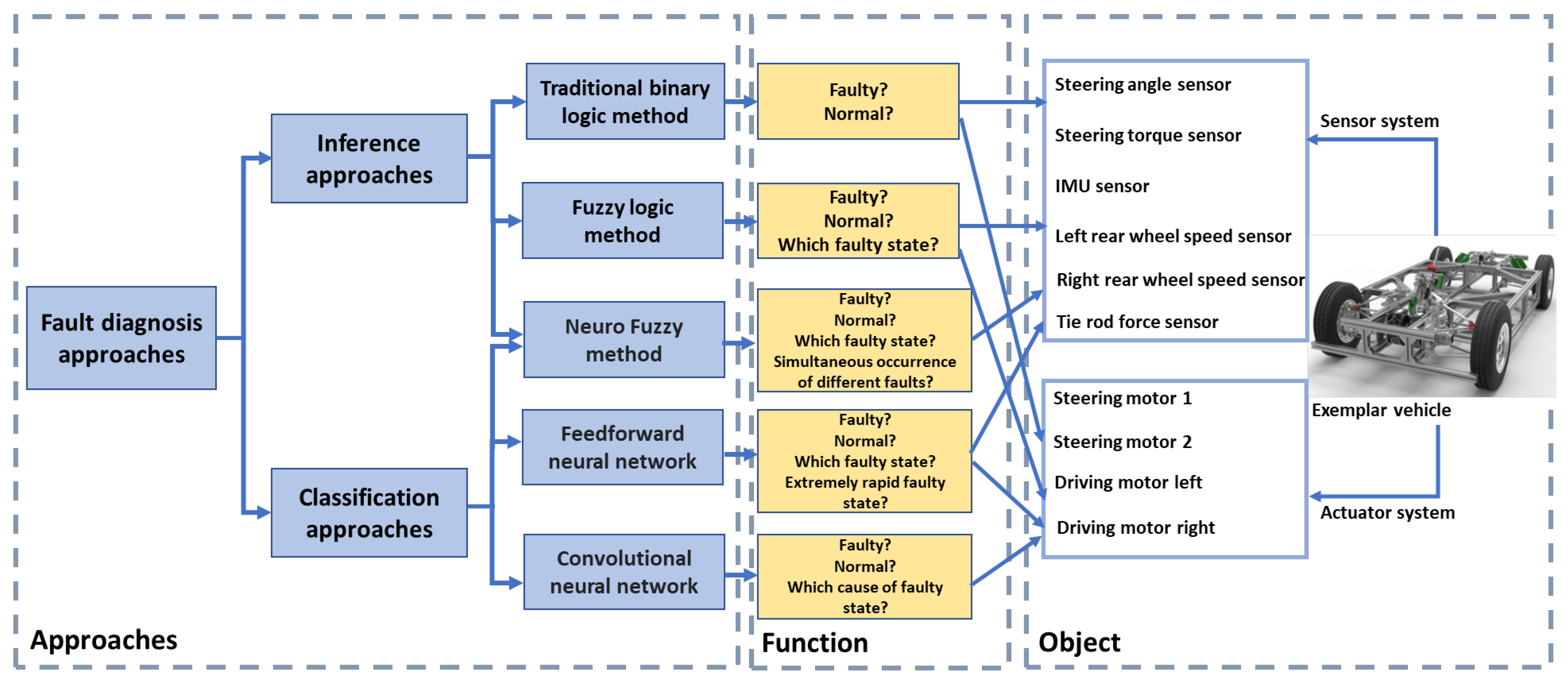
In this section, the fault diagnosis algorithm for the exemplar sensor system was built using the fuzzy logic method. The six sensors and their four fault states (positive offset, negative offset, total loss, and outlier) were involved. Since the rule bases of Mamdani fuzzy inference systems are more intuitive and simpler to comprehend, the Mamdani system was utilized here for fault diagnosis. The fuzzy logic algorithm is divided into five steps: fuzzification of the input signals, application of the fuzzy operator in the antecedent, the implication from the antecedent to the consequent, aggregation of the consequents across the rules, and defuzzification which comprise the fuzzy inference process.

As the input of the fuzzy logic system, there are eight residual values, the difference between the sensor-measured data and model-estimated data: $r_{{\delta }_S}$ (the residual of the steering wheel angle), $r_{M_S}$ (the residual of the steering wheel torque), $r_{\dot{\psi }}$ (the residual of the yaw rate), $r_{F_{TieRodSum}}$ (the residual of the tie rod force), $r_{v_{rl}}$ (the residual of the left rear wheel speed with geometric model), $r_{v_{rr}}$ (the residual of the right rear wheel speed with geometric model), $r_{v_{rl\_KF}}$ (the residual of the left rear wheel speed with Kalman filter), $r_{v_{rr\_KF}}$ (the residual of the right rear wheel speed with kalman filter). For the specific calculation method, please refer to the authors’ above-mentioned paper [18]. In the Mamdani fuzzy inference system, the first step is to transform the numerical value into a linguistic term and determine its degree of membership between 0 and 1. For example, three trapezoidal membership functions, “residual increase,” “residual zero,” and “residual decrease”, were applied here to fuzzify the input signals. Experimental results of the simulation chose the threshold for each function. After fuzzifying the inputs, the degree to which each antecedent component is satisfied for each rule was determined. The AND operator was utilized to obtain a single integer representing the result of the rule’s antecedent when the rule’s antecedent contains many components. In addition, the output signal’s membership function must be determined, and here four triangle membership functions were used, corresponding to the fault types “positive offset”, “non-fault”, “negative offset”, and “total loss”. They are used to convey the diagnostic outcomes for each sensor. Aggregation is the process of combining the fuzzy sets representing each rule’s outputs into a single fuzzy set. MAX was the aggregating method used in this paper. The aggregate output fuzzy set is the input for the defuzzification process, and the output is a single number. The chosen defuzzification method was the middle of maxima (MOM), namely, the middle of elements with maximum membership value. Each output signal from the defuzzification process indicates if a fault is present in the specific sensor. Furthermore, the type and the time-varying behavior can be determined through the waveform of the output signals.

Since there are four types of sensor faults and no faults are involved in the fault diagnosis of the sensor, the final output of the fuzzy logic is a definite number. Here, we determined that “1” represents “positive offset fault”, “−1” indicates “negative offset fault”, “−2” corresponds to “ total loss fault”, and “0” is “no-fault”. An outlier fault requires no special number because it can be judged from the resulting shape.

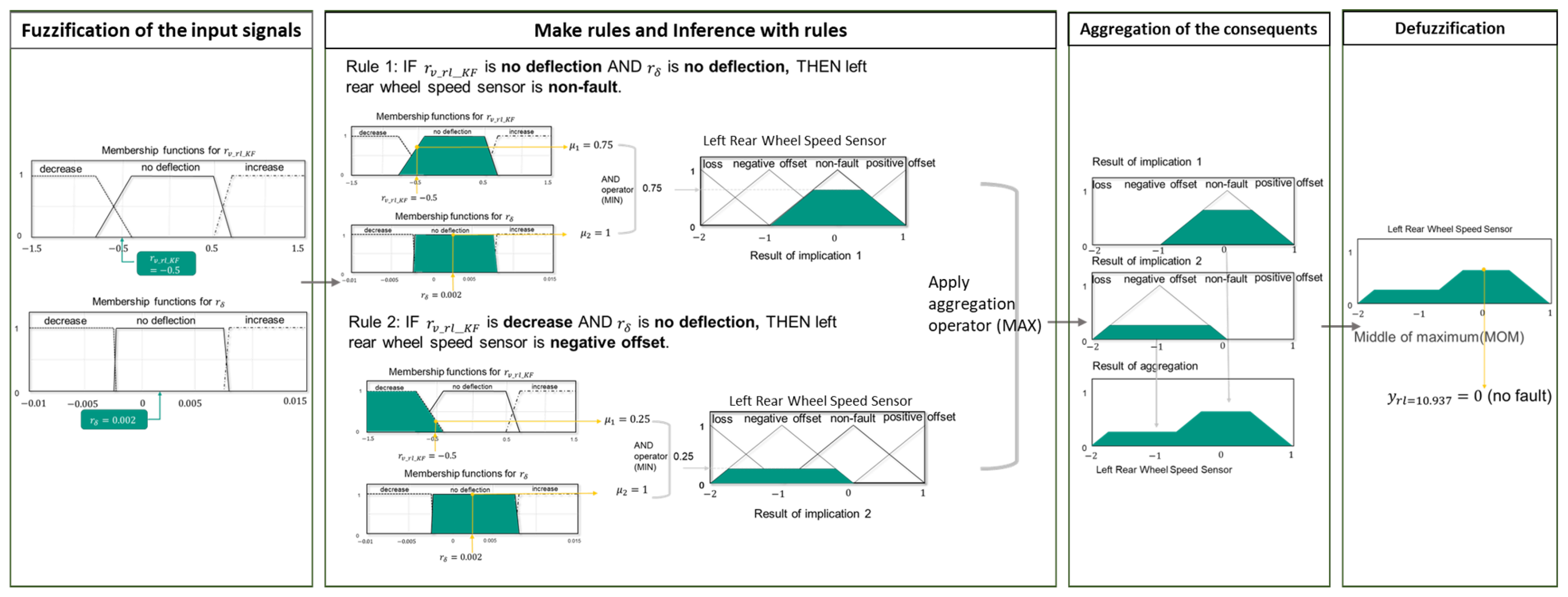
Here we use an example to illustrate the reasoning process of fuzzy logic more vividly. The entire reasoning process for this example is shown in Figure 2. First, we get two residual values: $r_{v_{rl\_KF}}=-0.5$ and $r_{{\delta }_S}=0.002$. For these two residuals, we first determined their membership functions with the help of the simulated data, which correspond to the two membership function diagrams in the leftmost box in Figure 2. When their membership functions are determined, the following two rules are formulated for them:

Rule 1: If $r_{v\_rl\_KF}$ is no deflection AND $r_{\delta }$ is no deflection, THEN left rear wheel speed sensor is non-fault;

Rule 2: If $r_{v\_rl\_KF}$ is decrease AND $r_{\delta }$ is no deflection, THEN left rear wheel speed sensor is negative offset;

The inference results of the two rules can be seen in the second box in Figure 2. It demonstrates that, by rule 1, the membership function corresponding to residual value $r_{v\_rl\_KF}$ is 0.75, whereas the membership function corresponding to residual value $r_{\delta }$ is 1. The outcome of applying the AND operator to the results of the two membership functions is then 0.75. According to this criterion, the probability that a sensor would not fail is 0.75. When matching to rule 2, the membership function for residual value $r_{v\_rl\_KF}$ is 0.25, and the membership function for residual value $r_{\delta }$ is 1. The outcome of applying the AND operator to the results of the two membership functions is 0.25. In other words, according to this criteria, the likelihood that the sensor has a negative deviation defect is 0.25. Merge the results of the two rules, and then use the MOM approach to defuzzify. The ultimate diagnosis result is 0, which indicates that the sensor is not defective.

2.1.2. Fuzzy Logic Diagnosis Algorithm for Exemplar Actuator System

In this chapter, we will introduce the fuzzy logic technique for actuator fault diagnosis. Two steering motors, two driving motors, and five states for each motor are included (no fault, small fault, middle fault, large fault, and total loss). The method of applying fuzzy logic enables the diagnostic to assess not only whether the system’s state is faulty but also the fault’s severity.

The fault diagnosis algorithm based on fuzzy logic techniques is the next step in model-based fault detection. It initially calculates the intended driving states using a mathematical model, including side-slip angle, yaw rate, target steering angle, target speed, etc. By comparing the ideal driving states to the actual driving states, which are measured by sensors, a set of residuals is calculated, which are the essential symptoms for fault diagnosis. The detailed process for calculating residuals is described in paper [18]. The key discussion here is the content of the fault diagnosis after getting the fault symptoms. For actuators, developing a fuzzy diagnostic algorithm is the same as for sensors. The Mamdani inference is still used. The method for defuzzification is the center of gravity. It determines the data’s central position as the output result of the fuzzy system. This method can provide a more objective estimate of the fault’s severity by considering the general distribution of the data.

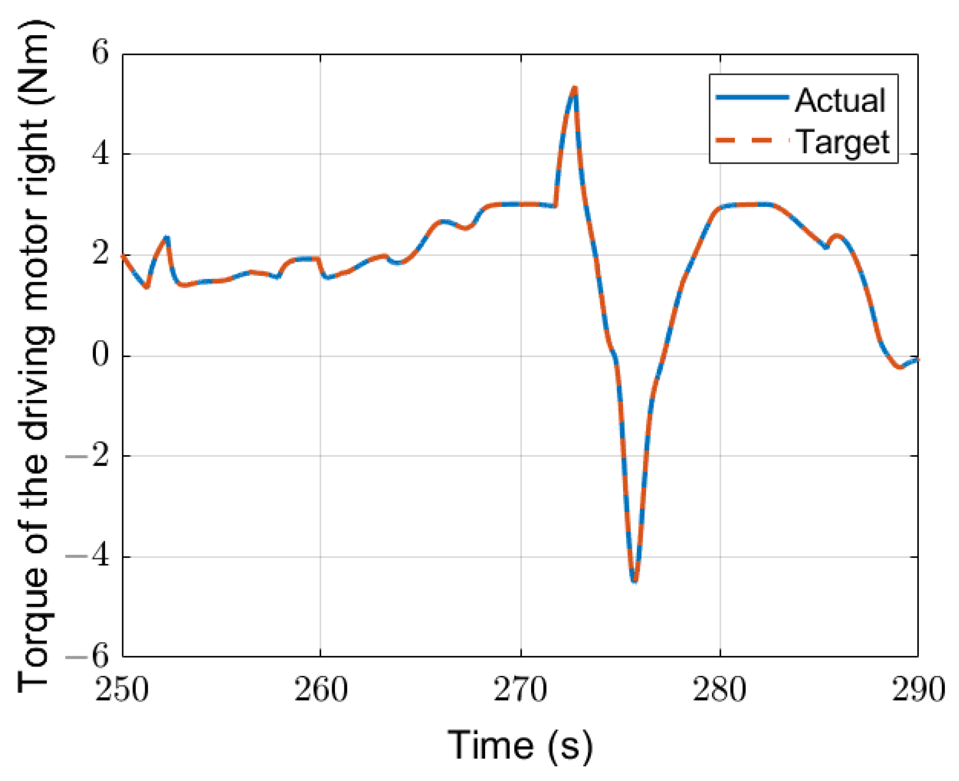
When diagnosing the steering system, the residuals we used include $r_{\dot{\psi }}$ (the difference between the target yaw rate and actual yaw rate), $r_{\beta }$ (the difference between the target side slip angle and actual side slip angle), $r_{{\delta }_S}$ (the difference between the target steering angle and actual steering angle), $r_{M_{LA1}}$ (the difference between the target steering torque and actual steering torque of the steering motor 1), $r_{M_{LA2}}$ (the difference between the target steering torque and actual steering torque of the steering motor 2). The fault diagnosis algorithm for the two driving actuators is similar to that for the two steering motors. Here mostly two residuals are employed as the symptoms of the fault diagnosis for determining the driving motor’s fault severity: $r_{v_x}$ (the difference between the target speed and actual speed) and $r_{F_{Tierod}}$ (the difference between the ideal tie rod force and the actual tie rod force). Among them, the speed residual is utilized to assess the presence of a fault, and the tie rod force residual is used to diagnose the severity of the motor fault.

2.1.3. Results of Fuzzy Logic Diagnosis Algorithm

(1)

Case a: Results of Fuzzy Logic Diagnosis For Sensors

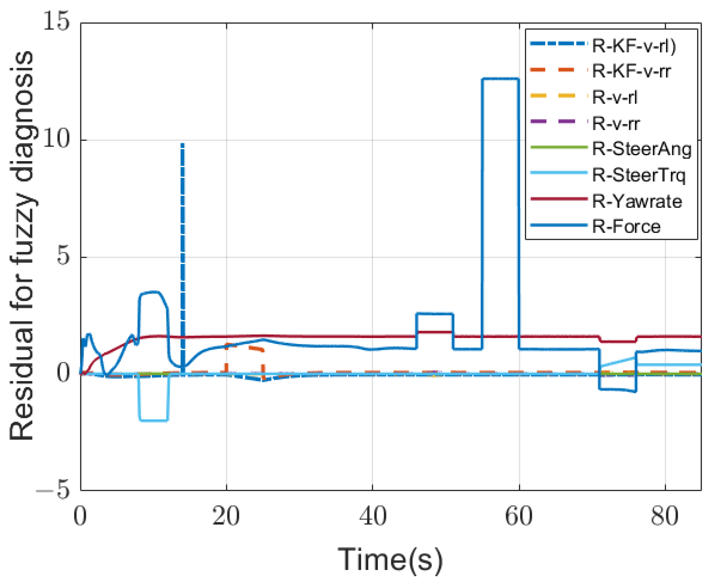
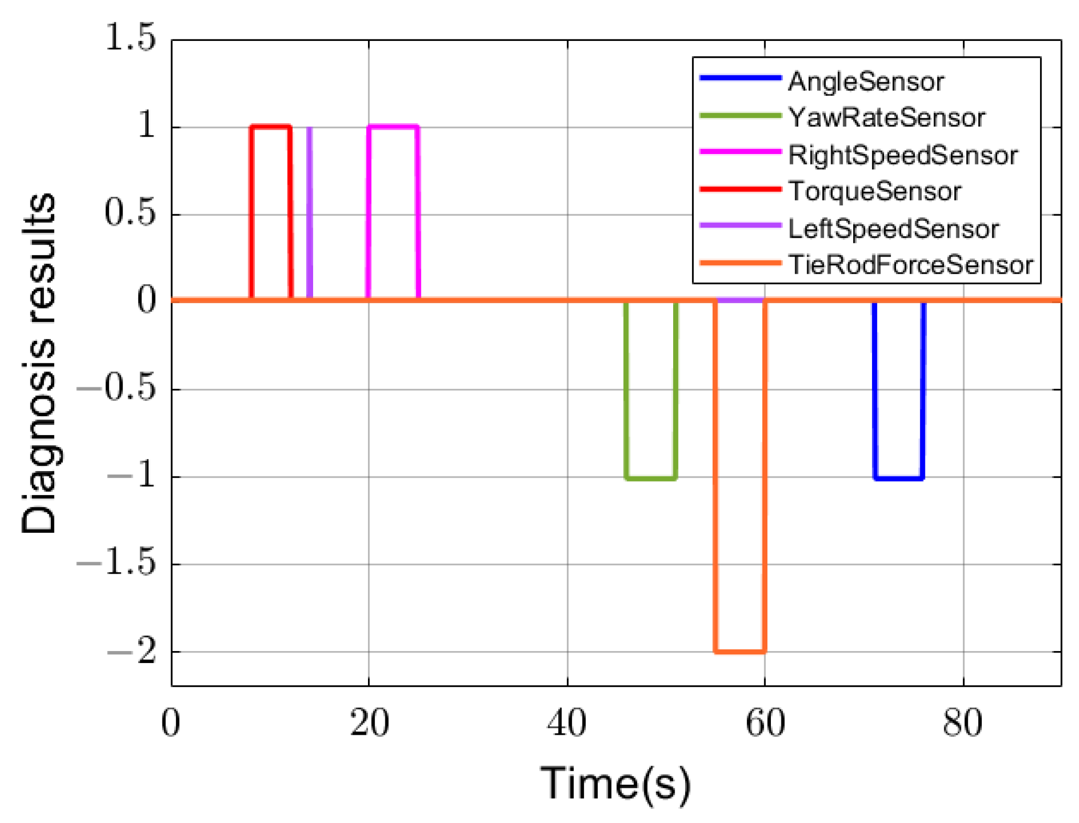
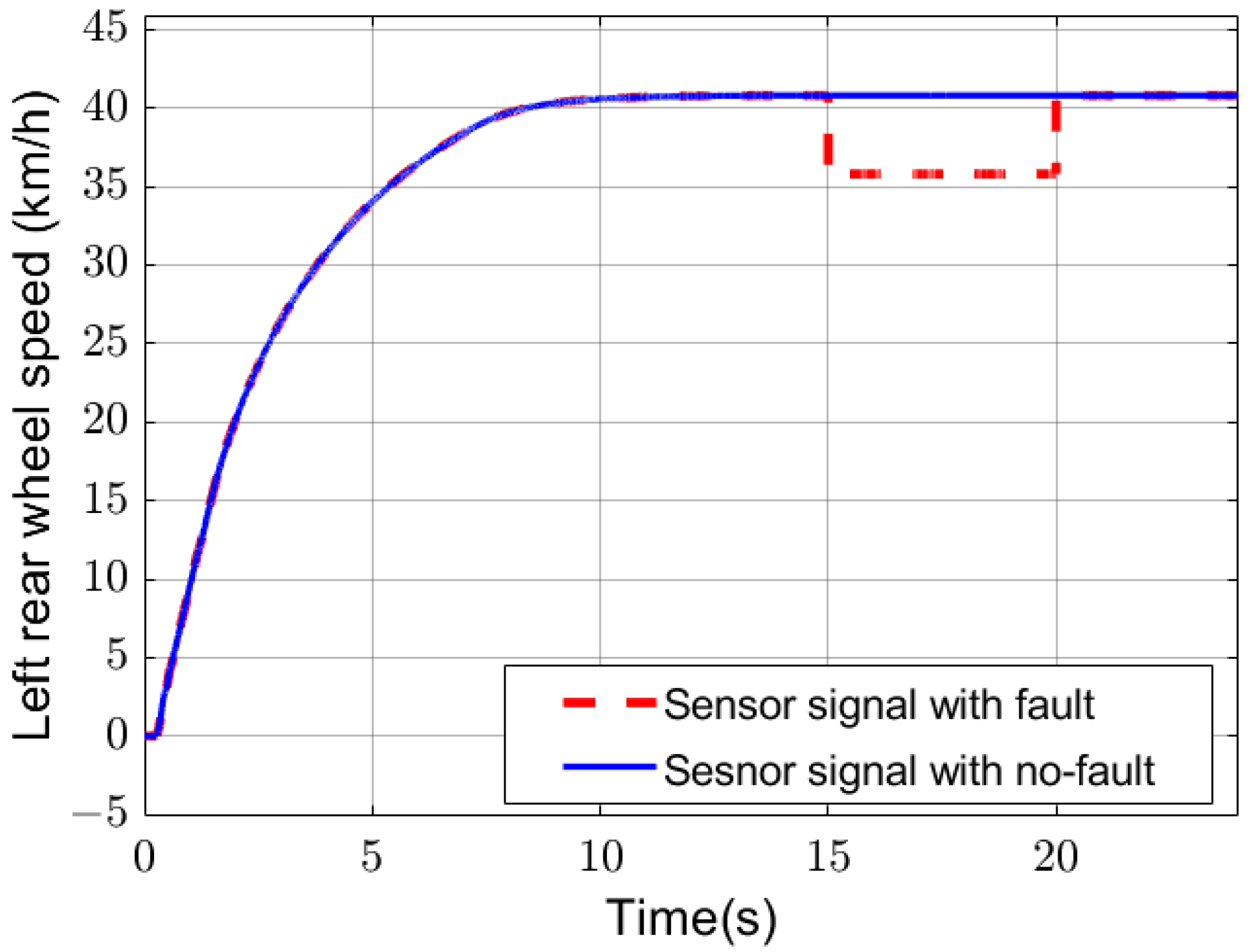
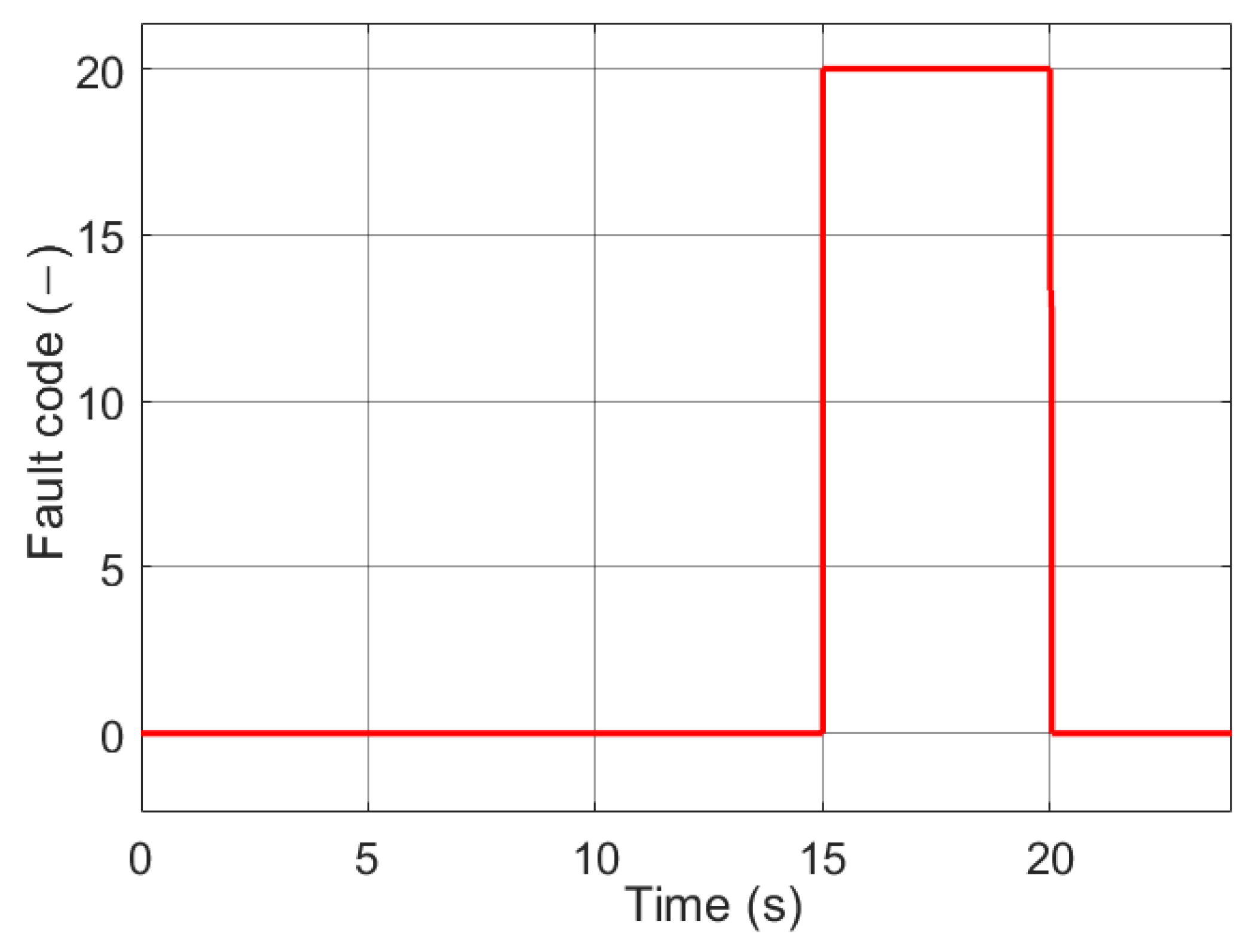
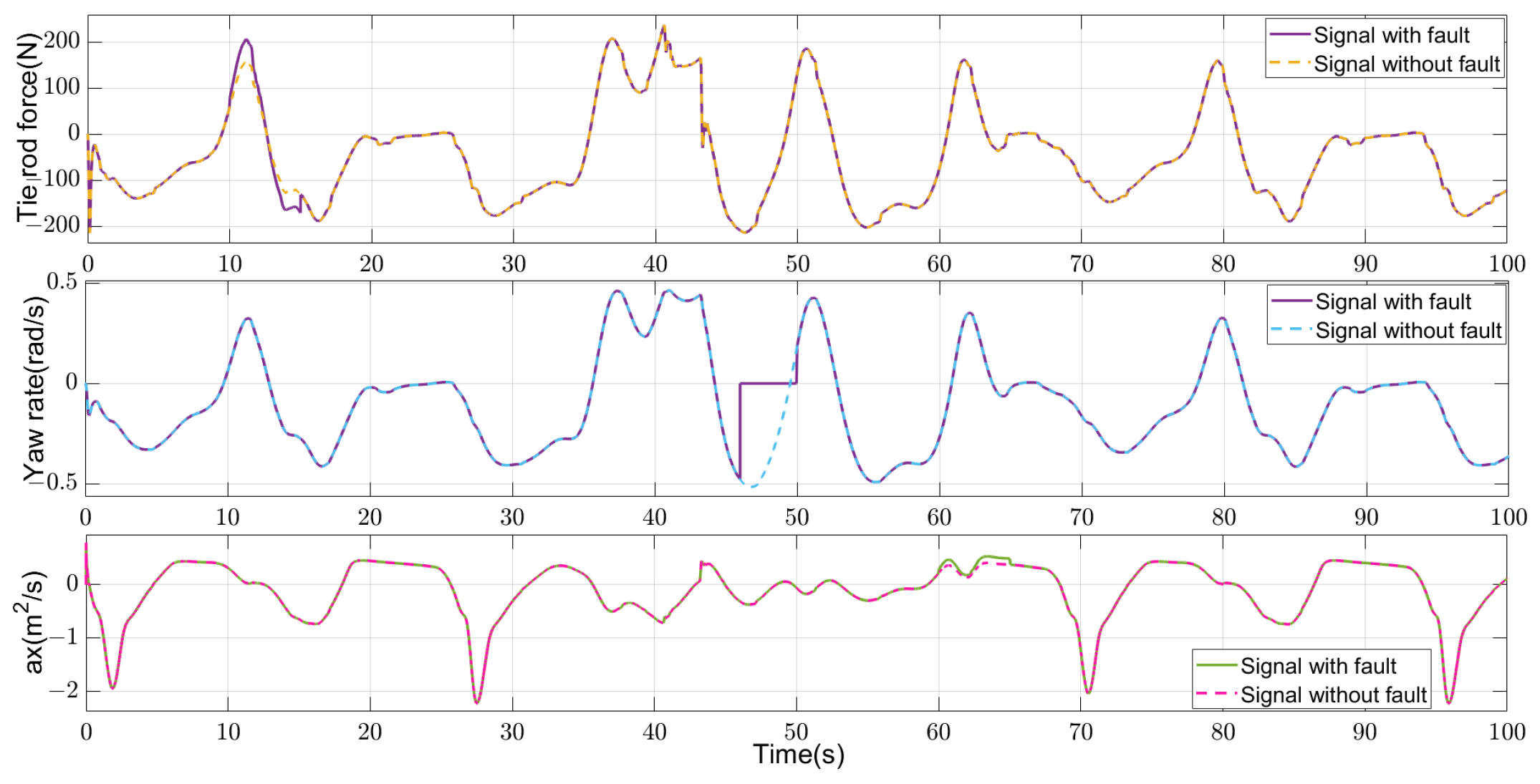
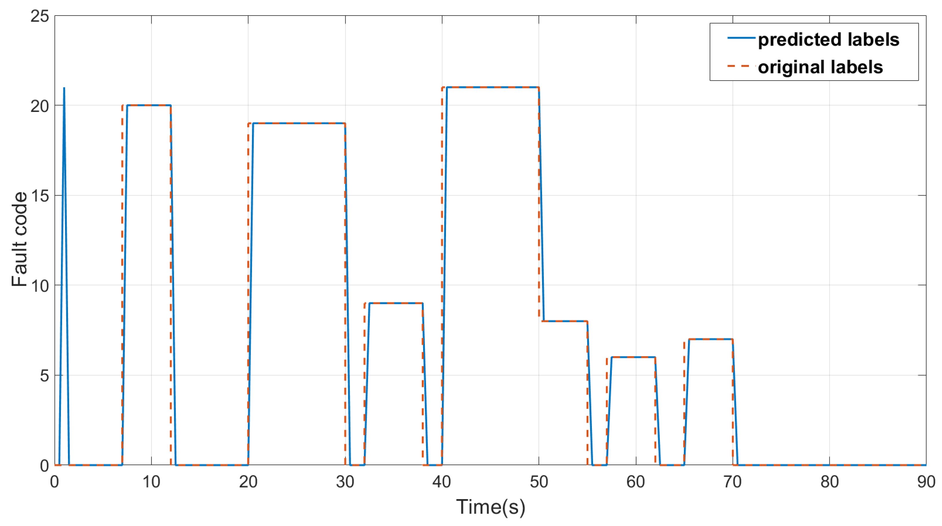
An example of sensor fault diagnosis results is shown in Figure 3 and Figure 4. In this test, we used a steady circular test with a radius of 24 m, and a fault injected at each sensor. There is a positive offset fault (fault code +1) in the steering wheel torque sensor between 8 and 12 s, an outlier fault in the left wheel speed sensor that only lasted 0.001 s at 14 s, a positive offset fault in the right wheel speed sensor between 20 and 25 s, a negative offset fault (fault code −1) in the yaw rate sensor between 46 and 51 s and a total loss fault (fault code −2) in the tie rod force sensor between 55 and 60 s, a negative offset fault in the steering wheel angle sensor between 71 and 76 s. Figure 3 shows the eight residual values used as inputs for fuzzy logic diagnosis, which have obvious changing trends within the corresponding fault injection periods. After the fuzzy logic diagnosis, we can get the six sensor diagnosis results, as shown in Figure 4. In this test, the six faults in the six sensors can be detected very accurately.

(2)

Case b: Results of Fuzzy Logic Diagnosis For Steering Actuators

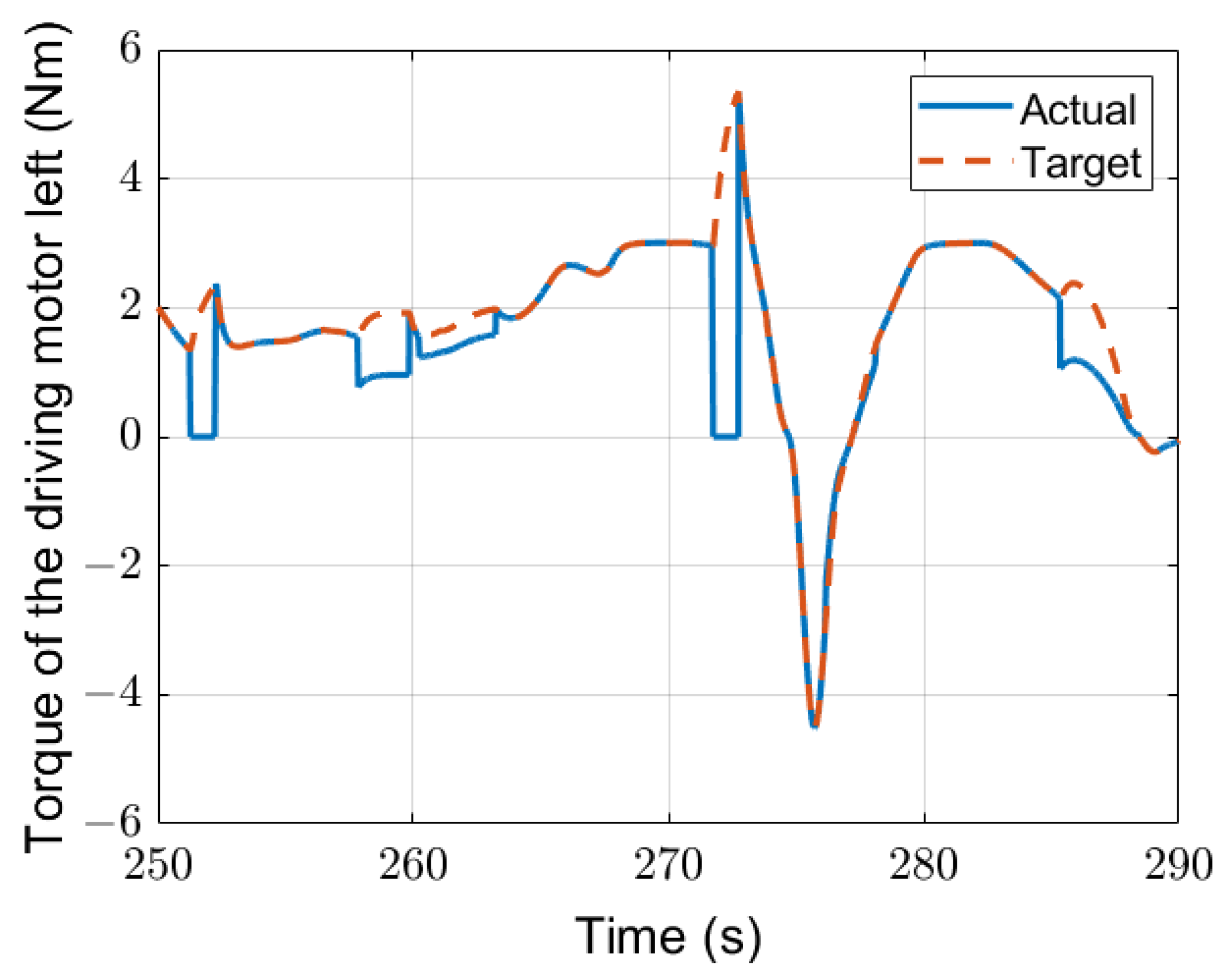
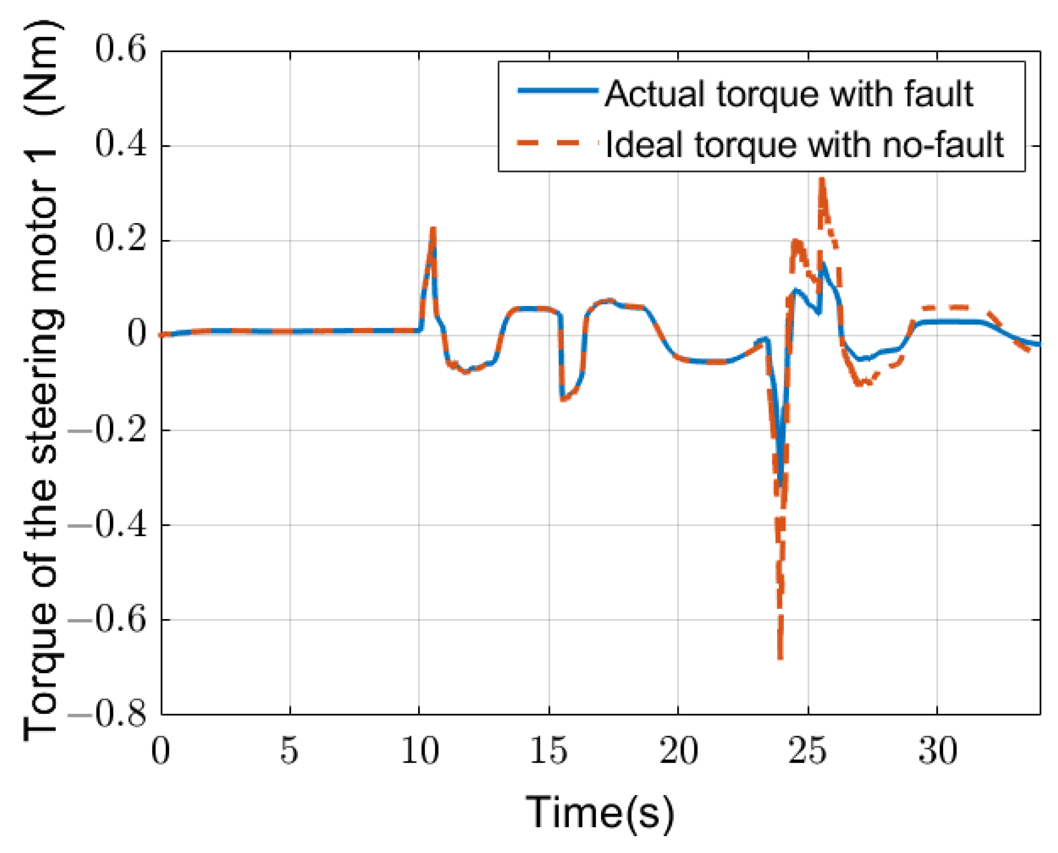
Figure 5 and Figure 6 show an example of the diagnosis result of a double lane change test for evaluating the fault diagnosis for actuators. The test vehicle is driven on the road at its maximum speed of 20 km/h for 34 s. There is a fault beginning at the 23 s that lasted until the end. The fault injected here is a Middle-Fault (50% target torque can be output). In this test, only steering motor 1 is operational. Figure 5 depicts the difference between the ideal torque and the actual output torque beginning at 23 s when the steering motor fails and cannot produce the needed torque. 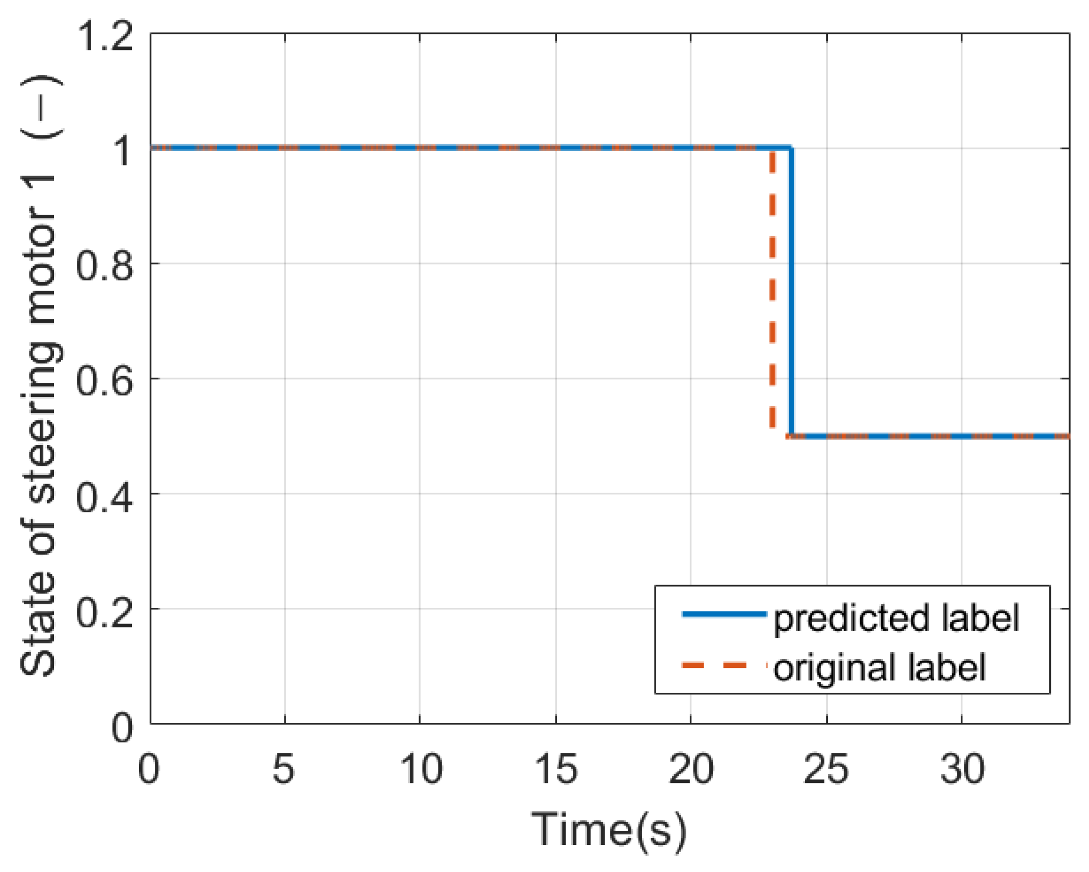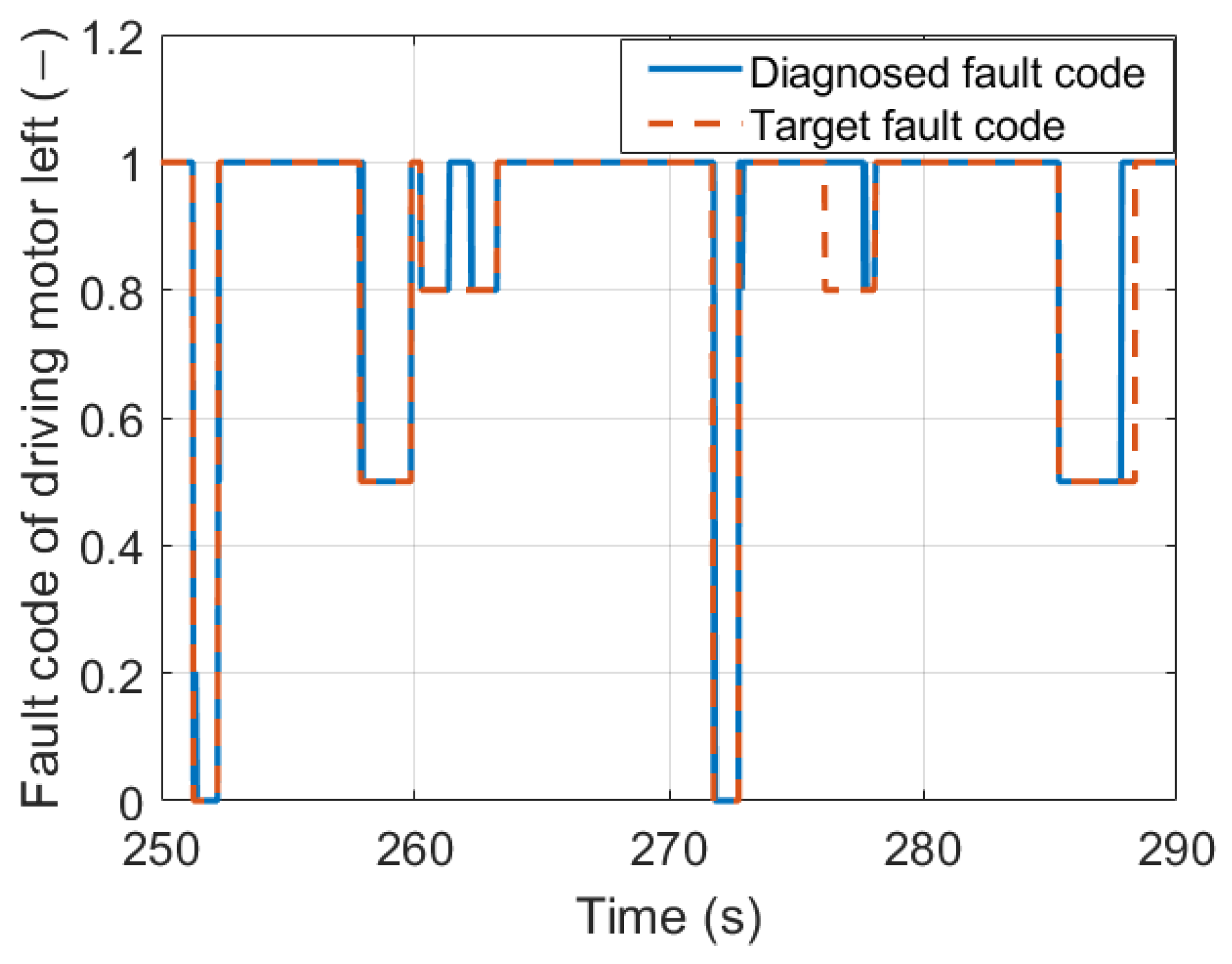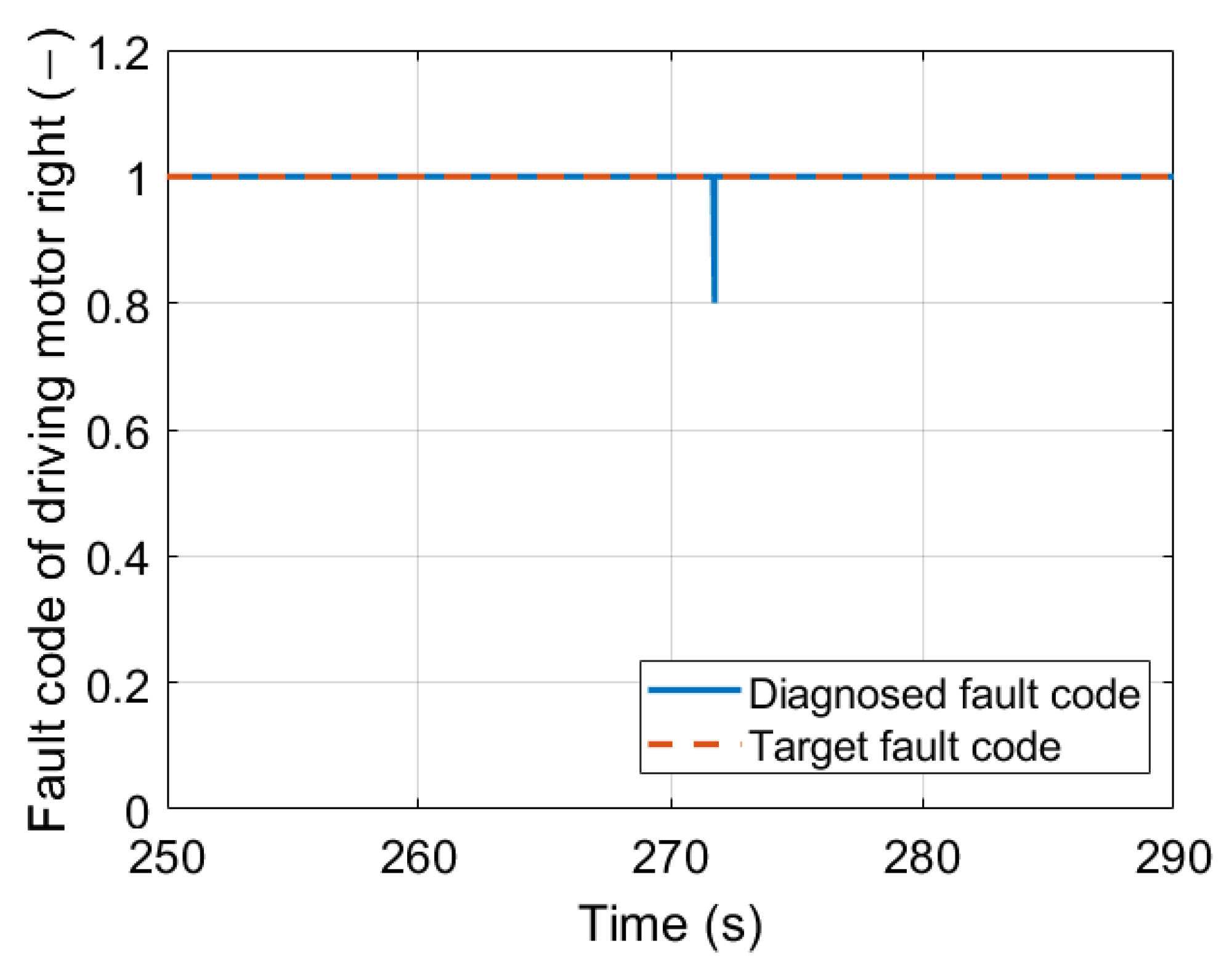Figure 6 depicts the result of the fuzzy logic fault diagnosis (blue line). 1 indicates that the motor is operating normally. At 23.6 s the diagnosis result changes to $0.5$ until the end, indicating that the present motor has a malfunction of medium severity. The fault occurred at 23 s. However, the faulty diagnosis was delayed by approximately 0.6 s. This is because, at 23 s, the anticipated steering torque is quite small. Even if a fault occurred, the resulting vehicle dynamic deviation is within the permitted range, diagnostics considered the actuator in a no-fault state.

The fault diagnosis algorithm based on fuzzy logic developed here can establish the fault’s type, location, and time-varying behavior if present in any of the sensors and actuators. This approach uses the generated residuals by mathematical models of the vehicle as its foundation. In response to modifying symptom vectors, a fuzzy logic system was implemented for fault diagnostics. The fuzzy logic outputs showed the type, location, and time-varying behavior of a defect. This method is very effective in diagnosing the fault state of a single sensor and the actuator fault severity.

2.2. Fault-Diagnosis Model Architecture Based on Neuro-Fuzzy

A neuro-fuzzy system employs fuzzy logic to model linguistic rules and neural networks to learn from data and modify the modeled rules. The neuro-fuzzy in the fuzzy modeling research field is divided into two areas: fuzzy linguistic modeling that is focused on interpretability, mainly the Mamdani model, and precise fuzzy modeling that is focused on accuracy, mainly the Takagi–Sugeno–Kang (TSK) model. Sugeno fuzzy inference employs singleton output membership functions that are either constants or linear functions of the input values. The defuzzification process for a Sugeno system is more computationally efficient than that of a Mamdani system. Moreover, the fuzzy rules and corresponding functions of Sugeno fuzzy inference can be automatically optimized using parameter learning. Based on the above characteristics, the Sugeno model is more suitable for neuro-fuzzy algorithms.

2.2.1. Neuro-Fuzzy Diagnosis Algorithm for Exemplar Sensor System

The steps for implementing TSK in neuro-fuzzy are as follows. Firstly, determine the input and output variables, as well as the input membership functions. Then create a collection of fuzzy rules for the TSK model, with each rule containing antecedents and consequences. Antecedents may consist of a single input variable or a mixture of numerous input variables, whereas the consequence is a linear function. Thirdly, construct a neural network that learns the TSK model’s parameters. The input layer of the neural network is comprised of the input variables, while the output layer is made up of the consequent functions of the fuzzy rules. Then apply fuzzy rules to the input variables and aggregate the outputs using the maximum-minimum composition or weighted average composition approach. The neural network is used to optimize the linear parameters of the fuzzy rules.

The object of fault diagnosis in this chapter is still six sensors, each with four fault types. In addition, it will also improve the diagnosis of multi-sensor faults, which are not involved in fault diagnosis using traditional fuzzy logic methods. Due to the employment of a Sugeno-type fuzzy inference system with a single numerical output, the outcome of this project’s diagnosis method is a fault code. Every sensor fault type is assigned a fault code on every sensor, which can be used to determine the fault type and location. Outlier faults are not assigned fault codes since their transient time behavior allows them to be identified.

Table A1. Fault code for single sensor fault.

	Positive Offset	Negative Offset	Total Loss
Steering wheel angle	1	2	3
Steering wheel torque	4	5	6
Yaw Rate	7	8	9
Wheel speed RL	10	11	12
Wheel speed RR	13	14	15
Tie rod force	16	17	18

in Appendix A contains the fault codes for the single-sensor fault scenarios, whereas

Table A2. Fault code for multi-sensor fault.

	Yaw Rate (PO)	Yaw Rate (NO)	Yaw Rate (TL)
Steering wheel angle (PO)	1	2	3
Steering wheel angle (NO)	7	8	9
Steering wheel angle (TL)	13	14	15
	Wheel speed RL (PO)	Wheel speed RL (NO)	Wheel speed RL (TL)
Steering wheel torque (PO)	4	5	6
Steering wheel torque (NO)	10	11	12
Steering wheel torque (TL)	16	17	18
	Wheel speed RL (PO)	Wheel speed RL (NO)	Wheel speed RL (TL)
Yaw Rate (PO)	19	20	21
Yaw Rate (NO)	22	23	24
Yaw Rate (TL)	25	26	27

in Appendix A contains the fault codes for the multi-sensor fault scenarios. The multi-sensor fault tests mainly target the steering wheel torque sensor, yaw rate sensor, and left rear wheel speed sensor. The fault types mainly consider positive offset, negative offset, and total loss.

The Fuzzy logic toolbox software in Matlab provides an interactive app, “Neuro-Fuzzy Designer,” which is used in this project to train an adaptive neuro-fuzzy inference system (ANFIS). The approach of model construction is Subtractive Clustering. Subtractive Clustering considers data points to represent the center of a Gaussian distribution, and it determines which data points should serve as class centers and allocates other data points to the class centers that are closest to them. Subtractive Clustering has the advantage of being able to handle big datasets and achieve typically acceptable clustering results, which makes it simple to construct the model without rule number exponential explosion. Four crucial parameters must be set separately: influence range, squash factor, accept ratio and reject ratio. There are currently no effective instructions for setting the aforementioned basic parameters. Through a pair of training procedures, parameters are set to optimal values based on a variety of training samples that correlate to a variety of simulation tests. Here, the steady circle driving test is used for parameter debugging. The changes in the debugged parameters are shown in

Table 1. Training parameters of subtractive clustering.

Range of Influence	Squash Factor	Accept Ratio	Reject Ratio	MF number	RMSE
0.5	1.25	0.5	0.15	7	1.056
0.3	1.25	0.5	0.15	15	0.389
0.2	1.25	0.5	0.15	23	0.163
0.1	1.25	0.5	0.15	24	0.106
0.1	1.25	0.5	0.1	26	0.027

, and the RMSE (Root-mean-square deviation) is used as the evaluation standard. A smaller range of influence and reject ratio will yield more membership functions and fuzzy rules, but training error RMSE will be reduced. However, this progress will approach a ceiling, meaning that increasing the number of membership functions and fuzzy rules will not lower training error but simply influence training speed. A smaller squash factor minimizes the likelihood that outlying points would be deemed part of a cluster, resulting in typically more and smaller data clusters. The accept ratio is a numeric value between 0 and 1 and must be greater than the rejection ratio. After importing the training data and building the initial FIS structure, the “Train FIS” portion opts for a hybrid optimization strategy in the training process that combines backpropagation with least-squares regression (LSE). Epochs are the number of training epochs and represent one complete cycle of the training data. This number is set between 10 and 20 for this project to converge the training error. Error tolerance is the training termination condition. When error tolerance is set to 0, training will end when the specified number of training epochs is reached. The inputs used here are eight residual values that are the same as those used in the diagnosis algorithm based on fuzzy logic.

2.2.2. Results of Neuro-Fuzzy Diagnosis

(1)

Case a: Results of Neuro-Fuzzy Diagnosis For Single Sensor Fault

Figure 7 depicts a total loss fault on the left rear wheel speed sensor during a round driving test. Here, the FIS is generated with a range of influence of 0.05, a squash factor of 1.25, an accept ratio of 0.5, and a reject ratio of 0.05, and a total of 52 membership functions. The blue line depicts the original signal from the left rear wheel speed sensor, whereas the red line represents the signal with a fault. At 30 s, a total loss fault is added to the sensor, and the value of the signal for the left rear wheel speed remains 0 until the end. Figure 8 depicts the matching fault code of the diagnosis result. Initially, the output remains 0, indicating no problem occurred during this period. After 30 s, the fault code changes to 12, corresponding to the total loss fault in the left rear wheel speed sensor, see Table A1 and remains until the end.

(2)

Case b: Results of Neuro-Fuzzy Diagnosis For Multi-Sensor Faults

In the ANFIS method, one of the very important advances is that it can identify multiple faults in multiple sensors. Figure 9 and Figure 10 depict a multi-sensor fault involving the left rear wheel speed sensor and the yaw rate sensor. Figure 9 depicts the left rear wheel speed sensor signal with a negative offset fault between 15 s and 20 s, whereas Figure 10 depicts the yaw rate sensor signal with a positive offset fault between 15 s and 20 s. Figure 11 depicts the diagnostic fault code output. Beginning with a fault code of 0, indicating that no fault has occurred, a fault code of 20 indicates that the left rear wheel speed sensor has a negative offset fault and the yaw rate sensor has a positive offset fault simultaneously at 15 s as shown in Table A2. The fault code lasts for 5 s before reverting to 0 until the end.

The adaptive neuro-fuzzy inference system is used to model the fault diagnosis algorithm for the exemplar sensor system. It possesses the interpretability of fuzzy logic and the parameter self-learning ability of artificial neural networks. This approach could diagnose the fault types in the sensors, and it has a good adaptive ability for complex driving maneuvers. In addition, the method is used to verify the possibility of diagnosis when multiple sensors fail simultaneously.

2.3. Fault-Diagnosis Model Architecture Based on Neural Networks

The rapid advancement of machine learning in recent years has made it advantageous for classification. In this section, fuzzy logic has been substituted by a neural network model based on a faulty dataset. Using historical data of the system under normal and various fault situations to train neural network models for fault diagnosis is the fundamental concept underlying machine learning approaches for fault diagnosis. In the event of a process failure, the machine learning algorithm requires exceptionally rich sample data, and the accuracy is highly dependent on the completeness and representativeness of these samples.

2.3.1. Feedforward Networks Diagnosis Algorithm for Exemplar Sensor System

The most prevalent neural network fault diagnosis methods are the two facets: utilizing neural networks to develop state observers and utilizing neural networks as a diagnostic classifier. The neural network observer is trained using data collected when the system is operating normally. Fault residuals can be generated using a trained neural network observer [21,22]. If the potential fault categories of a system have been classified beforehand, the difficulty of fault diagnosis becomes determining which class the current system state belongs to. That is the second technique, which uses neural networks for pattern recognition during fault diagnosis. The neural network classifier receives the current system state online and compares it with offline-obtained reference fault states to produce accurate diagnosis results. This method can be utilized for the fault diagnosis of process objects of the control system, as well as sensors and actuators [7,8].

In 1943, McCulloch and Pitts described the “M-P neuron model,” which is still in use today [23]. In this model, a neuron receives input signals from n other neurons, these input signals are transmitted through a weighted connection, and the total input value received by the neuron is compared to its threshold value before being processed by an activation function to generate the neuron’s output. The optimal activation function is the step function, which transfers the input value to “0” or “1” as the output value. 1 correlates to neuron excitement, and 0 to neuron inhibition. Nevertheless, the step function has discontinuous, non-smooth, and undesirable characteristics. Hence, the Sigmoid function is frequently utilized as the activation function. Input values that fluctuate within the range are squashed into the (0, 1) output value range. Two layers of neurons can comprise the perceptron. The input layer receives and sends the external input signal to the output layer. For the nonlinear problem, functional neurons with multiple layers (hidden layers) must be considered. The neural networks used in practical applications are trained with the backpropagation algorithm. The forward propagation algorithm calculates the network’s output first, followed by the output error in the backpropagation algorithm. The mistake is then propagated backwards to each neuron, and the gradient of each neuron is determined to determine the direction and magnitude of the network parameter adjustment. Lastly, to minimize network output error, the network parameters are changed using the gradient descent approach.

Here, the residual between the real measured data of the sensor and the sensor data estimated by the model is still an important input quantity for the machine learning model. After obtaining the residuals, a classification model should be applied to fault diagnostics. It accepts the sensor parameters previously acquired as input and outputs the discrete fault type. For the fault diagnosis of the aforementioned six sensors, the following residuals must be input: $r_{{\delta }_S}$ (the residual of the steering wheel angle), $r_{M_S}$ (the residual of the steering wheel torque), $r_{\dot{\psi }}$ (the residual of the yaw rate), $r_{F_{TieRodSum}}$ (the residual of the tie rod force), $r_{a_x}$ (the residual of the longitudinal acceleration), $r_{a_y}$ (the residual of the lateral acceleration), $r_{v_{rl}}$ (the residual of the left rear wheel speed), $r_{v_{rr}}$ (the residual of the right rear wheel speed). However, these residuals only indicate the absolute magnitude and not the relative value of the deviance. Consequently, it is essential to supply the input with the current measured values of the sensor: ${\delta }_S,M_S,\dot{\psi },F_{TieRodSum},a_x,a_y,v_{rl},v_{rr}$. Therefore, there are in total 16 parameters that we use as input when diagnosing sensor faults. In the obtained dataset, the training set accounts for 70%, and the validation set and test set each account for 15%. The total number of training samples used as a sensor fault diagnosis model is 184,862, each with 14 features.

Determined here are the number of hidden layers of the neural network, the number of neurons in each hidden layer, the activation function of the neurons, and the neural network training technique. Increasing the number of hidden layers in a neural network can improve classification performance but at the expense of a substantial increase in computation, a decrease in system speed, and the possibility of over-fitting. Since the inputs are values (and not images), only one hidden layer is necessary. The number of neurons in the buried layer is determined empirically. Based on testing, the categorization model employing the following empirical formula performs better:

$$n_{\mathrm{hidden}}=2\times n_{\mathrm{input}}-1$$

(1)

where $n_{\mathrm{input}}$ is the number of inputs, which is 16. Therefore, the number of neurons in the hidden layer is 31.

For models that use predicted probabilities as output, since probabilities can range from 0 to 1, the Sigmoid function is a good fit:

$$f\left(x\right)=\frac{1}{1+e^{-x}}$$

(2)

The Scaled Conjugate Gradient Backpropagation (SCG) is chosen for training. It is a development of the conjugate gradient method that dynamically modifies the step size during the optimization process using a scaling factor.

The number of model outputs should correspond to the number of sensor fault categories. Because the neural network can determine more types of faults, we can consider the IMU as two sensors: the yaw rate or the longitudinal/lateral accelerations, $a_x$ and $a_y$. Here only one sensor failure at a time is considered; each sensor has four failure modes, and there are 28 different modes of fault for all sensors. Outlier issues are no longer within the scope of diagnosis here to simplify the complexity of the model because this technique frequently produces an outlier, which will be confused with an outlier fault. Thus, there are 21 different fault types, corresponding to 22 codes from 0 to 21. The fault code for each type of fault is shown in

Table A3. Fault code for sensor fault based on machine learning.

	Positive Offset	Negative Offset	Total Loss
Steering wheel angle	1	2	3
Steering wheel torque	4	5	6
Yaw rate	7	8	9
Longitudinal acceleration	10	11	12
Wheel speed RL	13	14	15
Wheel speed RR	16	17	18
Tie rod force	19	20	21

. The output is an array of 22 bits with a total value of 1. The highest of these 22 values is selected, indicating that the most probable sensor defect type is selected.

2.3.2. Feedforward Networks Diagnosis Algorithm for Exemplar Actuator System

Two coaxially coupled steering actuators and two driving actuators are involved here. The fault diagnosis algorithms can diagnose five states of each actuator. The diagnosis algorithm’s inputs are the vehicle controller’s target values rather than the measured values. Target values can be viewed as the driver’s control commands and are the values the vehicle should reach. It consists of the steering wheel angle target ${\delta }_{S_{target}}$, the vehicle velocity target $v_{x_{target}}$, the two steering motors target torque $M_{L{A}_1\mathrm{target}}$, $M_{L{A}_2\mathrm{target}}$, and the drive motor target torque of the front left and right wheels $M_{F{L}_{target}},M_{F{R}_{target}}$. Similar to the sensor component, the input comprises residuals and actual values that can reflect both absolute and relative variances. Such inputs include $r_{v_x}$ (the difference between the target speed and actual speed), $v_x$ (the actual speed), $r_{a_x}$ (the difference between the target longitudinal acceleration and actual longitudinal acceleration), $a_x$ (the actual longitudinal acceleration), $r_{a_y}$ (the difference between the target lateral acceleration and actual lateral acceleration), $a_y$ (the actual lateral acceleration), $r_{\dot{\psi }}$ (the difference between the target yaw rate and actual yaw rate), $\dot{\psi }$ (the actual yaw rate), $r_{\beta }$ (the difference between the target side slip angle), and $\beta$ (the actual side slip angle). The other input is $PT{T}_{LA,total}$, which represents the percentage difference between the actual value and the intended value of the steering motor’s total steering torque. These 11 variables are the input of the fault diagnosis for the steering motor. Here the classifier requires only one hidden layer, which is comprised of 21 neurons. The activation function and training algorithm is identical to the sensor function and algorithm. There are five neurons in the output layer, which correspond to no fault, and four fault kinds for steering motors (Small fault: Only 70% to 90% of the target torque can be output; Middle fault: Only 40% to 60% of the target torque can be output; Large fault: Only 10% to 30% of the target torque can be output; Total loss fault: 0% of the target torque can be output). The total number of training samples used as a model for steering motor fault diagnosis is 554,406, and each set of samples has 11 features.

This study also significantly raises the bar for the classifier’s output threshold. “Miss” and “False alarm” definitions are crucial to fault diagnosis issues. “Miss” indicates that the positive sample is not correctly recognized, a “missed diagnosis.” A false alarm represents a response to a non-existent positive sample, a “misdiagnosis.” A compromise is required since it is challenging to decrease miss and false alarms in the same model. When the threshold is high, only extremely specific fault conclusions are produced, or the fault is ignored. Therefore, the false alarm rate is quite low, but the miss rate is relatively high. When the threshold is low, all suspected faults are output. So the false alarm rate is high, and the miss rate is low. The diagnosed results will have a significant impact on the vehicle’s regular operation. The goal is to find a method to report the faults infrequently (fewer false alarms) but necessarily (fewer missed alarms). The steering motor has little impact when the car is driving straight. A higher threshold allows some less critical problems to be overlooked. The steering motor is essential when the car steers. A lower threshold needs to be applied to maximize fault diagnosis accuracy. In this study, a basic logic gate is proposed to ascertain if the car is now steering or traveling straight. The vehicle can virtually be thought of as traveling straight: if ${\delta }_S$ is small $AND$ $\dot{\psi }$ is small $AND$ $\beta$ is small $AND$ $a_y$ is small, at which point a high threshold is employed to get more missed alarms and less false alarms. Otherwise, the car is thought to be steering using a low threshold to achieve fewer missed and more false alarms.

As with the steering motor input, the input of the drive motor fault diagnosis model consists of 10 vehicle state reflecting parameters: $r_{v_x}$, $v_x$, $r_{a_x}$, $a_x$, $r_{a_y}$, $a_y$, $r_{\dot{\psi }}$, $\dot{\psi }$, $r_{\beta }$, $\beta$. Also useful are the total tie-rod force and its residual: $F_{TieRodSum}$, $r_{F_{T}ieRodSum}$. The total tie-rod force is a valuable diagnostic parameter for the driving motor. Because there should be theoretically no significant change of $F_{TieRodSum}$ when the vehicle is traveling in a straight line, $F_{TieRodSum}$ exists when the vehicle steers. So if $F_{TieRodSum}$ deviates significantly from the estimated value, that is, a driving motor fault may also be suspected. In addition, the input also includes the target torques of the two drive motors from the vehicle controller. There are a total of 14 inputs. The model’s output layer contains a total of 9 neurons, which corresponds to no faults and four fault states for each driving motor. The total number of training samples used as a model for driving motor fault diagnosis is 554,406, and each set of samples has 14 features. The drive motor’s significance is influenced by two variables: acceleration $a_x$ and current velocity $v_x$. When a drive motor fault occurs, high $v_x$ is more hazardous for the driver than low $v_x$. In addition, vehicle acceleration is achieved by the working of the driving motor, so completing the diagnosis should be more necessary when the vehicle accelerates. A higher threshold should be utilized if “$v_x$ is small OR $a_x$ is small” so that the false alarm rate is lower and the miss rate is higher. Otherwise, a lower threshold was applied, resulting in a greater false alarm rate but a lower miss rate.

2.3.3. Results of Neural Networks Diagnosis Algorithm

(1)

Case a: Results of Neural Networks Diagnosis Algorithm For Sensors

Figure 12 depicts an example test result of faulty sensors. In this test, we injected seven faults in the sensors. There was a positive offset fault in the tie rod force sensor between 10 s and 15 s (fault code 19), a negative offset fault in the steering wheel torque sensor between 30 s and 35 s (fault code 5), a total loss fault in the yaw rate sensor between 46 s and 50 s (fault code 9), a positive offset fault in the longitudinal acceleration sensor between 60 s and 65 s (fault code 10), a negative offset fault in the left wheel speed sensor between 70 s and 74 s (fault code 14), a negative offset fault in the right wheel speed sensor between 80 s and 85 s (fault code 17) and a total loss fault in the steering wheel angle sensor between 95 s and 98 s (fault code 3). As shown in Figure 12 (blue line), the sensor fault diagnosis system can deliver mostly accurate results. However, there are still weaknesses. It can be seen from the diagnosis results that there are some outliers, and these outliers can be removed through a filter without affecting the overall diagnosis results. However, at the same time, there are still some missed diagnoses, such as the tie rod force sensor diagnosis at 12 s, the yaw rate sensor diagnosis at 49 s, and the longitudinal acceleration fault diagnosis at 60 s. To know the reason for its missed diagnosis, it is necessary to rely on the raw sensor data, as shown in Figure 13. The reason for the missed diagnosis is related to the threshold. Utilizing a threshold guarantees that the problem diagnosis system only returns a result when it is pretty definite. This minimizes incorrect diagnoses at the expense of a rise in missed diagnoses. At these missed diagnosis periods, the real values of the sensors are very small, close to 0. This confuses the fault detection system, as the changes in features generated by the three separate fault kinds are similar in the dataset used to train the neural network. When the actual value is close to zero, the significance of the corresponding sensor diminishes. Therefore, an appropriate missed diagnosis is also acceptable.

(2)

Case b: Results of Neural Networks Diagnosis Algorithm For Driving Actuators

Here is an example of the diagnosis of the actuator system. It is difficult to obtain the output torques of the two drive motors. However, the fault diagnosis of the drive motor still provides nearly accurate diagnosis results, thanks to the addition of two new features: total tie rod force $F_{TieRodSum}$ and its residual $r_{FTieRodSum}$. The estimation model specifies the goal value of $F_{TieRodSum}$, indicating that, according to acceptable calculations, $F_{TieRodSum}$ should be close to 0 or a constant when the vehicle is traveling straight or a specified value when the vehicle is steering. If one of the drive motors fails at this moment, there will be an immediate loss of power on the corresponding side, resulting in an additional “steering” effect.

Figure 14, Figure 15, Figure 16 and Figure 17 show the result of an example test of fault diagnosis for the two driving motors. In this test, the front left drive motor fails between 250 and 290 s during driving. Six faults with different magnitudes and duration times are injected in the left front driving motor within the period indicated by the red dotted line in Figure 16. The blue lines in Figure 16 and Figure 17 demonstrate that the fault diagnosis results for the driving motors and provide the right conclusions in the majority of situations, and the more severe the fault, the higher the accuracy of the diagnosis. For instance, there will be two missed diagnoses for ”Small-Fault” that occurred between 260.5 and 263.5 and between 276 and 278 s. Since “Small” problems have little effect on the driving safety of a vehicle, the performance of the drive motor fault diagnosis system is satisfactory. It can be seen from the diagnosis result that the neural network diagnosis approach is very sensitive to short-term faults.

The fault diagnosis approach based on feedforward neural networks proposed in this section has adequate diagnostic capabilities. It can diagnose seven sensor states and three fault types for each sensor. For the exemplar actuator system, it can also diagnose the states of the four actuators, and each has five states, for a total of 20 types of states for the actuator system. This approach can suitably apply to extremely short-term fault scenarios, and it has strong adaptability for a quick response to short-term fault scenarios and an accurate diagnosis result.

2.4. Fault-Diagnosis Model Architecture Based on CNN

Convolutional neural network (CNN) is a unique artificial neural network in deep learning. In various fields, such as manufacturing, transportation, and healthcare, CNN has proven to be a potent tool for fault diagnosis in recent years. In electric vehicles, the motor plays a crucial role, and motor malfunctions always have a significant effect on driving behavior. When a fault occurs, timely maintenance is required. Determining the precise cause of motor malfunctions is thus an essential task. The permanent magnet synchronous motor is the most frequently used actuator in electric vehicles. It has a fairly simple overall construction. However, when the motor runs, certain components will deteriorate and fail over time with prolonged operation due to the influence of power supply circumstances, load conditions, and the operating environment. The most common fault causes include eccentricity of the motor rotor, winding disconnection, winding overheating, inter-turn short circuits, insulation age, etc. The rotor of the permanent magnet synchronous motor likewise has a permanent magnet, so irreversible demagnetization is also possible. With the developed CNN models in this case, four fault causes can be found: open-switch fault, short-switch fault, short circuit between phases fault, and permanent magnet demagnetization fault. The CNN approach will identify 21 fault states refined differently across four fault kinds and one no-fault state.

2.4.1. CNN Diagnosis Algorithm for PMSM

The input layer, convolutional layer, pooling layer, and fully connected layer constitute the majority of the layers of a conventional convolutional neural network. The input layer of a convolutional neural network receives the original data or the data obtained after preparation. Through the input layer, the convolutional neural network is fed input data for feature extraction. The convolutional layer is the central component of CNN, which can extract the local features of the input data via the convolution kernel. Due to the property of automatic feature extraction, using CNN can naturally reduce the difficulty of manually preprocessing raw data. The convolution kernel slides onto the input data so that the local area is convolved with the convolution kernel. This procedure can be interpreted as utilizing the kernel to filter each small section of the picture to extract its eigenvalues. The eigenvalues of each region are then used to generate a feature map. The number of feature mappings is commensurate with the number of convolution kernels. The sliding stride is an essential parameter for controlling the size of the output feature map during the sliding process. The purpose of the pooling layer is to minimize the data’s dimensionality and prevent overfitting. The fully connected layer is responsible for processing the data processed by the convolutional layer and the pooling layer to reach the final desired result.

As depicted in Figure 18, the CNN model presented in this section for diagnosing the causes of the faults in PMSM consists of an input layer, a convolutional layer, a pooling layer, two fully connected layers, and an output layer.

The activation function used here is the Softmax function. It is also a typical activation function appropriate for multi-classification issues in which the categories are mutually exclusive. Softmax maps the output of many neurons to the $(0,1)$ interval, which may be thought of as the likelihood that the current output belongs to each category. The softmax activation function formula is illustrated in Equation (3). K denotes the number of motor fault kinds. $x_i$ and $x_j$ indicate the output values of the $i$-th and j-type motor faults before Softmax normalization, and $f\left(x_i\right)$ reflects the output value after normalization or the likelihood of a certain type of motor fault.

$$f\left(x_i\right)=\frac{e^{x_i}}{{\sum }_{j=1}^K{e}^{x_j}}.$$

(3)

CNN is typically referred to as a two-dimensional neural network, but a one-dimensional convolutional neural network is also useful when we want to extract important features from shorter (fixed-length or kernel-size) segments of the entire dataset, and the feature is not highly correlated with the location of the segment of data. In addition, time series analysis of sensor data, such as that from an accelerometer or gyroscope, can benefit from using 1D CNN. Since the original data for this paper were gathered from several sensor data groups by time series, 1D CNN was employed in the model. The parameters of the one-dimensional convolutional layer were Cov1D (*, 50, 64). * indicates that the number of samples entered can be any value. 50 indicates that the layer uses 50 convolution kernels for convolution operations. Each convolution kernel can extract a feature. 64 means that the size of the convolution kernel is 64. Each convolution operation selects 64 adjacent input neurons (or features) to perform convolution operations with the convolution kernel. There are numerous pooling techniques for CNN. Here we used maximum pooling. By dividing the input data into numerous rectangular sub-areas, maximum pooling outputs the maximum value for each sub-area. Convolutional and max-pooling layers must be transformed into one-dimensional layers and transferred to fully linked layers because they contain two-dimensional data. As fault detection of electric motors is the issue to be examined in this section, this model can forecast problems for 22 fault states (including one fault-free normal state). The 21 types of motor faults that can be diagnosed with their corresponding fault codes are shown in

Table A4. Types of motor faults for diagnosis based on CNN.

Fault Code	Motor Fault Cause
0	Both motors are working fine
1	Open switch fault in the inverters of both motors
2	Short switch fault in the inverters of both motors
3	Short circuit between phases of both motors
4	Demagnetization of both motors, the magnetic flux is 20% of the original
5	Demagnetization of both motors, the magnetic flux is 80% of the original
6	Open switch fault in the inverter of left motor
7	Short switch fault in the inverter of left motor
8	Short circuit between phases of left motor
9	Demagnetization of left motor, the magnetic flux is 0% of the original
10	Demagnetization of left motor, the magnetic flux is 20% of the original
11	Demagnetization of left motor, the magnetic flux is 40% of the original
12	Demagnetization of left motor, the magnetic flux is 60% of the original
13	Demagnetization of left motor, the magnetic flux is 80% of the original
14	Demagnetization of right motor, the magnetic flux is 0% of the original
15	Demagnetization of right motor, the magnetic flux is 20% of the original
16	Demagnetization of right motor, the magnetic flux is 40% of the original
17	Demagnetization of right motor, the magnetic flux is 60% of the original
18	Demagnetization of right motor, the magnetic flux is 80% of the original
19	Open switch fault in the inverter of right motor
20	Short switch fault in the inverter of right motor
21	Short circuit between phases of right motor

. It includes open switch faults, short switch faults, and phase-to-phase short-circuit faults of the inverters of the two motors separately and simultaneously, five different severe demagnetization states of the two motors respectively, and two severe demagnetization states of the two motors simultaneously. The output layer has 22 nodes. Each node’s output represents the predicted value obtained by the node, which can be regarded as the probability that the model believes that the corresponding fault occurs.

The dataset was still divided into three groups here, a training set, a validation set, and a test set = 6:2:2. The relevant vehicle driving parameters are the model’s input. The choice of parameters will affect the speed of model training and the correct rate of the model. To get a better result, we need first to visualize the original data, intuitively select all the parameters that change with the type of fault, and remove the parameters that have no feedback on the change of the fault type. For instance, a relevant component that must be included in the training model is the current, which will vary quite obviously when a fault occurs. Parameters that do not change considerably, like a car’s driving distance, can be disregarded. As the input for the final training, we chose 10 variables in this case. They are the driving torque on the tire, the d-phase current modified by the $dq$ coordinate system, and the currents of the $abc$ three phases in the motor’s three-phase circuit. There are two motors in the vehicle, one for each of the two front wheels, so 10 variables can be used. After selecting the relevant data variables, data preprocessing is also very important. Time series data can be preprocessed using a variety of techniques; however, sliding window pretreatment is crucial for maximizing the amount of data. Additionally, the sliding window may determine the window’s length on its own to make sure that each sample’s data dimension is consistent. The sliding window’s starting point during data preparation was randomly established to lessen the reliance between samples and time. Ultimately, a sample length of 50 and a total sample size of 45,360 were chosen.

2.4.2. Results of CNN Diagnosis for PMSM Failure Causes

Figure 19 shows the result of a test with multiple faults. This test contains eight states: non-fault, SSF in the inverter of the right motor, OSF in the inverter of the right motor, complete demagnetization of the rotor in the left motor, phase-to-phase short circuit in the right motor, phase-to-phase short circuit in the left motor, SSF in the inverter of the left motor, OSF in the inverter of the left motor, as the corresponding fault code shown in Table A4. A comparison chart between the predicted results (blue line) and the original labels (red line) is produced when the prediction model receives the first sample. Even if the results are as expected, there will be a delay of 0.5 s. The fault diagnosis (kind, location, and duration) in this test is always accurate, except for the tiny mistake which occurred because of the starting of the car. The accurate rate is 95.44%.

The proposed model’s capacity to differentiate between negative and positive samples is so robust that it excels in diagnosing motor faults. The 22 types of situations (1 normal working state, 21 fault states) that will occur in the motors in electric vehicles can be identified. The algorithm is used to conduct a real-time diagnosis of multiple faults, which is closer to practical applications. In a given operating condition, the motor has 2 to 8 different operating states, and the classification accuracy of the model can reach 90% or more, up to 95%.

3. Evaluation of the Different Methods

In Section 2, we outlined five distinct fault diagnosis techniques and modeled corresponding diagnosis algorithms for the respective exemplar systems. Then these methodologies are evaluated in this chapter. One of the most important evaluations for fault diagnosis methods is the accuracy of fault diagnosis. However, as long as enough test data are provided, enough diagnostic circumstances are made, or enough modeling and computations are consumed, any approach, whether it be conventional binary logic fault diagnosis or the popular neural network technology, may eventually reach quite a good accuracy of the diagnosis. For comparing several methods, it makes no sense to neglect other assessment criteria and concentrate exclusively on fault diagnostic accuracy. Therefore, we did not evaluate the single fault diagnosis rate in this instance; rather, we evaluated these five fault diagnosis approaches more in terms of the pros and cons of the method itself, as well as any applicable circumstances and scenarios.

Traditional binary logic fault diagnostics can accurately assess whether the system is normal or abnormal. Different logic gates and logical operation symbols can create a variety of diagnostic criteria between symptoms to locate the faulty part. The diagnostics are traceable and explainable due to the rules’ transparency. This strategy also has clear drawbacks. It requires lengthy simulation and testing and just returns a faulty or non-faulty result and cannot give further diagnostic information, like fault type or severity. The fuzzy logic fault diagnosis approach extends the classical logic approach. It can handle ambiguous fault information. This method mimics how humans process fuzzy information, making it more realistic. Practical fault information is incomplete, inaccurate, and imprecise. Fuzzy logic theory can better represent and diagnose this information. As fuzzy logic picks numerous membership functions and reasoning techniques dependent on the situation, it may adapt to varied defect diagnostic scenarios. It can express more reasoning relations and concepts than binary logic fault detection. This approach can identify fault types and severity. The membership functions and inference procedures are manually formulated, significantly affecting the diagnosis outcomes. So selecting it is challenging and requires experienced experts or many experimental verifications. It involves a lot of fuzzy set operations and is computationally intensive. The approach may misdiagnose imprecise or unclear data. Hence, the diagnostic can have uncertain results. Neuro-fuzzy fault diagnostics uses a combination of neural networks and fuzzy logic. It can handle uncertain and fuzzy information, like fuzzy logic, for more complicated fault scenarios. Due to neural networks, model parameters may automatically adjust to different failure conditions. As a drawback, this technique needs plenty of training data. Otherwise, the accuracy and dependability would be doubted. Neuro-fuzzy fault diagnosis can produce confusing findings and is not suitable for situations that require explicit diagnostic rules. Feedforward neural network has a strong ability for fault diagnostics. It can model nonlinear systems. Adaptive learning from prior data improves diagnosis accuracy. It handles complicated failure scenarios and is robust for noise-resistant. It is also applicable to multivariable failures and systems. As a normal machine learning approach, it needs a lot of data to train the model. Convolutional neural networks have more powerful data processing capabilities than feedforward neural networks, which can be used for more complex fault situations. CNN’s convolutional and pooling layers automatically extract meaningful characteristics from incoming data. It can solve multivariable failure situations in complicated systems. End-to-end learning eliminates manual feature extraction and improves diagnostic efficiency. Nevertheless, a CNN model requires a lot of training data for accurate and reliable predictions. CNN is also a type of neural network, it requires sophisticated calculations and special resources, and parameter setting impacts diagnostic accuracy. Like the feedforward neural network diagnostics, it is not good at identifying failure causes with transparent inference.

The evaluation of each feature of these five fault diagnosis methods is shown in

Table 2. Evaluation of sixteen features of five fault diagnosis methods (”√” denotes an advantage of this approach in this characteristic, ”×” denotes a drawback of this approach in this feature, and ”-” sign denotes a combination of benefits and disadvantages in this aspect for this technique).

	Traditional Binary Logic Fault Diagnosis	Fuzzy Logic Fault Diagnosis	Neuro-Fuzzy Fault Diagnosis	Feedforward Neural Network Fault Diagnosis	Convolutional Neural Network Fault Diagnosis
Simple algorithm	√	×	×	×	×
Assess system abnormality	√	√	√	√	√
Identify fault type and severity	×	√	√	√	√
Traceability and interpretability	√	√	-	×	×
Model-building time consumption	×	×	×	√	√
Inference rule objectivity	-	×	-	√	√
Manage confusing fault messages	×	√	√	√	√
Various inferences	×	√	√	√	√
Experts needed	√	×	×	×	×
Auto-adjust model parameters	×	×	√	√	√
Requires numerous data	√	√	×	×	×
Needs particular computational resources	√	√	×	×	×
Handle non-linear fault conditions	×	-	√	√	√
Complex failure scenarios	×	√	√	√	√
Multivariate failure management	×	√	√	√	√
Situations needing a clear diagnosis inference	√	√	-	×	×

.

Figure 20 depicts a relative score for the application attributes of these five approaches, with 1 indicating the least suitable and 3 indicating the most appropriate. Traditional binary logic is ideally suited for circumstances where the system’s abnormality must be determined. Its traceability and explainability, as well as its straightforward and practical inference rules, are very significant advantages. In situations involving several sorts of faults, both fuzzy logic and neural networks are viable options. If explicit and transparent rules for inference are required, fuzzy logic is the best option. Neural networks are an excellent option when only accurate results are required, and high-performance computing tools are accessible. Neuro-fuzzy and neural networks are optimal for more complicated fault scenarios, such as multiple components failing simultaneously or short-duration faults. For limited input variables, neuro-fuzzy can be chosen. Initially, the rules are defined manually, and then the parameters are optimized automatically based on the data. Neural networks can be employed directly when dealing with extremely high input volumes. If more detailed fault information is required, such as the particular reason for failure, but no interest in developing too many mathematical models, the convolutional neural network is an excellent option. In conclusion, the best strategy to resolve the issue is to select the most appropriate diagnostic approach based on the various requirements, situations, and fault scenarios.

4. Conclusions

In this research, the authors modeled the fault diagnosis of sensor systems and actuator systems in electric vehicles using five fault diagnosis approaches. These five fault diagnosis methods are sorted from the traditional to the latest, namely, the traditional binary logic method, the fuzzy logic method, the neuro-fuzzy method, the feedforward neural network method, and the convolutional neural network method. The mathematical algorithms of the traditional binary logic method are simple and easy to create, the diagnostic rules are brief and clear, and it has good traceability and transparency. However, it only applies to simple fault scenarios and can only determine whether or not a system fault exists. It is used with the sensor system and actuator system to determine whether or not there is an anomaly and which part is abnormal in this study. The fuzzy logic technique is effective in handling ambiguous and fuzzy defect data. Because of the membership function, its diagnostic criteria are more varied and comprehensive. It may indicate not only whether there is a fault in the system but also its type and severity. Here, it is used to diagnose different sorts of faults in sensor systems and faulty components and their severity in actuator systems. Neuro-fuzzy is a combination of fuzzy logic and neural networks. It can first construct fuzzy rules based on experience or data and then use numerous datasets to improve the fuzzy rules’ parameters. As a result of the existence of neural networks, the interpretability, and traceability of the models deteriorate. It can be used in slightly more complex scenarios. Nevertheless, its variability is not as excellent as neural networks in the face of extremely complicated fault scenarios, and complex fault scenarios increase the complexity of constructing fuzzy rules. Therefore it must be chosen with caution. This approach is used in this research to diagnose the sensor system’s fault type. Owing to its automated parameter optimization, it is ideally suited for use in situations when many sensors fail simultaneously. Being the fundamental technique of machine learning, feedforward neural networks are ideally suited for fault diagnostics. It can also be sensitive to complicated driving circumstances and fault scenarios, such as extreme short-time faults lasting one or two seconds. Yet, the most prominent characteristic of machine learning is its inexplicability, which is unsuitable for scenarios that must rigorously describe the diagnostic procedure. A large quantity of data are required to ensure the algorithm’s stability. The approach is also utilized to diagnose the fault position and fault type of the sensor system, as well as the fault location and severity of the actuator system. Moreover, the diagnosis of complicated and dynamic fault scenarios, such as numerous faults in a test with long-term and short-term faults with varying lengths, is included. The convolutional neural network is more capable of processing data than the feedforward neural network, allowing it to diagnose more kinds of faults and classify them more precisely. In this article, convolutional neural networks were utilized to categorize the fault causes of permanent magnet synchronous motors, which have great diagnostic capabilities.

This study also evaluated these five fault-detection techniques and a recommendation to select alternative fault-detection techniques based on the diagnostic requirements of various circumstances. The research’s impartiality and efficacy may be best ensured by employing distinct diagnostic techniques based on usage situations, diagnostic criteria, or research goals. Currently, only simulated data have been used to validate our methodology. The goal of this paper is to evaluate the capabilities of different diagnostic methods in different application scenarios and fault diagnosis requirements. It is impossible to test complex fault scenarios, such as faults that last for 1 s or multiple faults in one test, or to inject as many different types of faults, such as sensor positive deviation faults and permanent magnet synchronous motor demagnetization faults, into the real vehicles. Therefore, there is a dearth of data that may be used to assist our study in the real car test. So, in this case, we only considered the verification of simulated virtual data. The author’s follow-up research will go into the verification of this relevant issue in actual vehicle testing.

References

1. Castillo, I.; Edgar, T. Model based fault detection and diagnosis. In Proceedings of the TWCCC Conference, Austin, TX, USA, 4–5 February 2008. [Google Scholar]
2. Meskin, N.; Khorasani, K. Fault Detection and Isolation: Multi-Vehicle Unmanned Systems; Springer Science & Business Media: Berlin/Heidelberg, Germany, 2011. [Google Scholar]
3. Bergman, S.; Astrom, K. Fault detection in boiling water reactors by noise analysis. In Proceedings of the 5th Power Plant Dynamics, Control and Testing Symposium, Knoxville, TN, USA, 21–23 March 1983. [Google Scholar]
4. Moseler, O.; Heller, T.; Isermann, R. Model-based fault detection for an actuator driven by a brushless DC motor. IFAC Proc. Vol. 1999, 32, 7873–7878. [Google Scholar] [CrossRef]
5. Kulkarni, M.; Abou, S.C.; Stachowicz, M. Fault detection in hydraulic system using fuzzy logic. In Proceedings of the World Congress on Engineering and Computer Science, San Francisco, CA, USA, 20–22 October 2009; pp. 20–22. [Google Scholar]
6. Fischer, D.; Börner, M.; Schmitt, J.; Isermann, R. Fault detection for lateral and vertical vehicle dynamics. Control Eng. Pract. 2007, 15, 315–324. [Google Scholar] [CrossRef]
7. Hussain, M.; Hassan, C.C.; Loh, K.; Mah, K. Application of artificial intelligence techniques in process fault diagnosis. J. Eng. Sci. Technol. 2007, 2, 260–270. [Google Scholar]
8. Saxena, A.; Saad, A. Fault diagnosis in rotating mechanical systems using self-organizing maps. In Artificial Neural Networks in Engineering (ANNIE04); Elsevier: Amsterdam, The Netherlands, 2004. [Google Scholar]
9. Panoiu, M.; Panoiu, C.; Lihaciu, I. Adaptive neuro fuzzy system for modelling and prediction of distance pantograph catenary in railway transportation. In Proceedings of the Materials Science and Engineering; IOP Conference Series; IOP Publishing: Bristol, UK, 2018; Volume 294, p. 012073. [Google Scholar]
10. Ballal, M.S.; Khan, Z.J.; Suryawanshi, H.M.; Sonolikar, R.L. Adaptive neural fuzzy inference system for the detection of inter-turn insulation and bearing wear faults in induction motor. IEEE Trans. Ind. Electron. 2007, 54, 250–258. [Google Scholar] [CrossRef]
11. Neue Methoden zur Zuverlässigkeitssteigerung von Hochautomatisierten Elektrischen Fahrzeugen (SmartLoad); Teilvorhaben: Szenarienbasierte Validierung von Hochautomatisierten Elektrischen Fahrzeugen. Available online: https://www.tib.eu/de/suchen/id/TIBKAT:1814793585/Neue-Methoden-zur-Zuverl%C3%A4ssigkeitssteigerung-von?cHash=ef5a165fa06a70762814601fc3ec1126/ (accessed on 27 September 2022).
12. Luo, H. Method Development for Fault Detection of Sensors in a Demonstrator Vehicle. Master’s Thesis, Karlsruhe Institute of Technology (KIT), Karlsruhe, Germany, 2021. [Google Scholar]
13. Meng, F. Modellbasierte Fehlererkennung der Aktoren eines Elektrischen Automatisierten Fahrzeugs. Master’s Thesis, Karlsruhe Institute of Technology (KIT), Karlsruhe, Germany, 2021. [Google Scholar]
14. Feng, Y. Optimization of the Robustness of a Holistic Fault Diagnosis System for an Electric and Automated Vehicle. Master’s Thesis, Karlsruhe Institute of Technology (KIT), Karlsruhe, Germany, 2021. [Google Scholar]
15. Hong, X. Validierung und Bewertung der Funktion Einer Fehlerdiagnosemethode. Master’s Thesis, Karlsruhe Institute of Technology (KIT), Karlsruhe, Germany, 2022. [Google Scholar]
16. Li, J. Implementation of AI Methods in a Holistic Fault Diagnosis System for an Electric and Automated Vehicle. Master’s Thesis, Karlsruhe Institute of Technology (KIT), Karlsruhe, Germany, 2022. [Google Scholar]
17. Yang, Z. Optimization of the Model-Based Fault Detection and Fuzzy-Logic-Based Fault Diagnosis of Sensors in a Demonstrator Vehicle. Master’s Thesis, Karlsruhe Institute of Technology (KIT), Karlsruhe, Germany, 2021. [Google Scholar]
18. Li, S.; Frey, M.; Gauterin, F. Model-Based Condition Monitoring of the Sensors and Actuators of an Electric and Automated Vehicle. Sensors 2023, 23, 887. [Google Scholar] [CrossRef] [PubMed]
19. Zadeh, L.A. Fuzzy sets. In Fuzzy Sets, Fuzzy Logic, and Fuzzy Systems: Selected Papers by Lotfi A Zadeh; World Scientific: Singapore, 1996; pp. 394–432. [Google Scholar]
20. Zadeh, L.A. The concept of a linguistic variable and its application to approximate reasoning—I. Inf. Sci. 1975, 8, 199–249. [Google Scholar] [CrossRef]
21. Simani, S.; Fantuzzi, C.; Spina, R. Application of a neural network in gas turbine control sensor fault detection. In Proceedings of the International Conference on Control Applications (Cat. No. 98CH36104), Trieste, Italy, 4 September 1998; pp. 182–186. [Google Scholar]
22. Fuente, M.; Represa, C. A comparative study of neural networks based approach for fault detection. IFAC Proc. Vol. 1997, 30, 471–476. [Google Scholar] [CrossRef]
23. Minsky, M.; Papert, S. Perceptrons; MITT Press: Cambridge MA, USA, 1969. [Google Scholar]
24. Wu, X. Method Development for Diagnosing the Causes of Faults in a PMSM. Master’s Thesis, Karlsruhe Institute of Technology (KIT), Karlsruhe, Germany, 2022. [Google Scholar]
Figure 1. Overview of the approaches and their applications in this paper.
Machines 11 00482 g001
Figure 2. Fuzzy process example.
Machines 11 00482 g002
Figure 3. The eight residual changing trends that are used as the inputs for fuzzy diagnosis.
Machines 11 00482 g003
Figure 4. An example of the diagnosis results for six sensors: steering wheel angle sensor with a negative offset (−1), yaw rate sensor with a negative offset (−1), right wheel speed sensor with a positive offset (+1), steering wheel torque sensor with a positive offset (+1), left wheel speed sensor with a positive offset (+1), and tie rod force sensor with a total loss (−2).
Machines 11 00482 g004
Figure 5. Torque of Steering actuator 1 (Blue line: the actual steering torque with faults; red dotted line: the ideal steering torque with no-fault).
Machines 11 00482 g005
Figure 6. The diagnosis result of the steering actuator 1 (Blue line: the diagnosis result; red dotted line: the original fault label).
Machines 11 00482 g006
Figure 7. Left rear wheel speed sensor signal (Blue line: sensor signal with no fault; red dotted line: sensor signal with a total loss fault).
Machines 11 00482 g007
Figure 8. Diagnosis output with a fault code 12, which corresponds to a total loss fault in the left rear wheel speed sensor at 30 s until the end.
Machines 11 00482 g008
Figure 9. Left rear wheel speed sensor signal (Blue line: sensor signal with no fault; red dotted line: sensor signal with a negative offset fault).
Machines 11 00482 g009
Figure 10. Yaw rate sensor signal (Blue line: sensor signal with no fault; red dotted line: sensor signal with a positive offset fault).
Machines 11 00482 g010
Figure 11. Diagnosis output with a fault code 20, which corresponds to a multi-fault of the left rear wheel speed sensor with a negative offset fault and the yaw rate sensor with a positive offset fault between the 15 to 20 s.
Machines 11 00482 g011
Figure 12. An example of the diagnosis results for six sensors: tie rod force sensor with a positive offset (19), steering wheel angle sensor with a negative offset (5), yaw rate sensor with a total loss (9), longitudinal acceleration with a positive offset (10), left wheel speed sensor with a negative offset (14), right wheel speed sensor with a negative offset (17) and steering wheel torque sensor with a total loss (3).
Machines 11 00482 g012
Figure 13. Sensor signal of tie rod force sensor, yaw rate sensor, and longitudinal acceleration (Solid line: Sensor signal with faults; dotted line: sensor signal without fault).
Machines 11 00482 g013
Figure 14. Torque of driving actuator left (Blue line: the actual steering torque with faults; red dotted line: the ideal driving torque with no-fault).
Machines 11 00482 g014
Figure 15. Torque of driving actuator right (blue line: the actual driving torque; red dotted line: the ideal driving torque).
Machines 11 00482 g015
Figure 16. The diagnosis result of the driving actuator left (Blue line: the actual diagnosis results, which presented six faulty states; red dotted line: the original fault label).
Machines 11 00482 g016
Figure 17. The diagnosis result of the driving actuator right (Blue line: the actual diagnosis results, which presented no fault of driving actuator right; red dotted line: the original fault label).
Machines 11 00482 g017
Figure 18. Proposed CNN model for diagnosis the fault causes of permanent magnet synchronous motor [24].
Machines 11 00482 g018
Figure 19. An example of the result of fault diagnosis for PMSM, which has eight fault states (Blue line: the predicted label with CNN model, red line: the original fault label): non-fault (0), SSF in the inverter of the right motor (20), OSF in the inverter of the right motor (19), complete demagnetization of the rotor in the left motor (9), phase-to-phase short circuit in the right motor (21), phase-to-phase short circuit in the left motor (8), SSF in the inverter of the left motor (7), OSF in the inverter of the left motor (6).
Machines 11 00482 g019
Figure 20. The ratings of the five fault diagnostic techniques for distinct attributes range from 1 (worst) to 3 (best).
Machines 11 00482 g020