Article

Methodology for Tool Wear Detection in CNC Machines Based on Fusion Flux Current of Motor and Image Workpieces

by
Geovanni Díaz-Saldaña
1,
Roque Alfredo Osornio-Ríos
1,
Israel Zamudio-Ramírez
1,2,
Irving Armando Cruz-Albarrán
1,
Miguel Trejo-Hernández
1 and
Jose Alfonso Antonino-Daviu
2,*
1
CA Mecatrónica, Facultad de Ingeniería, Campus San Juan del Río, Universidad Autónoma de Querétaro, Av. Río Moctezuma 249, San Juan del Río, Querétaro 76807, Mexico
2
Instituto Tecnológico de la Energía, Universitat Politècnica de València (UPV), Camino de Vera s/n, 46022 Valencia, Spain
*
Author to whom correspondence should be addressed.
Machines 2023, 11(4), 480; https://doi.org/10.3390/machines11040480
Submission received: 15 March 2023 / Revised: 5 April 2023 / Accepted: 12 April 2023 / Published: 14 April 2023
(This article belongs to the Section Advanced Manufacturing)

Abstract

:
In the manufacturing industry, computer numerical control (CNC) machine tools are of great importance since the processes in which they are used allow the creation of elements used in multiple sectors. Likewise, the condition of the cutting tools used is paramount due to the effect they have on the process and the quality of the supplies produced. For decades, methodologies have been developed that employ various signals and sensors for wear detection, prediction and monitoring; however, this field is constantly evolving, with new technologies and methods that have allowed the development of non-invasive, efficient and robust systems. This paper proposes the use of magnetic stray flux and motor current signals from a CNC lathe and the analysis of images of machined parts for wear detection using online and offline information under the variation in cutting speed and tool feed rate. The information obtained is processed through statistical and non-statistical indicators and dimensionally reduced by linear discriminant analysis (LDA) and a feed-forward neural network (FFNN) for wear classification. The results obtained show a good performance in wear detection using the individual signals, achieving efficiencies of 77.5%, 73% and 89.78% for the analysis of images, current and stray flux signals, respectively, under the variation in cutting speed, and 76.34%, 73% and 63.12% for the analysis of images, current and stray flux signals, respectively, under the variation of feed rate. Significant improvements were observed when the signals are fused, increasing the efficiency up to 95% for the cutting speed variations and 82.84% for the feed rate variations, achieving a system that allows detecting the wear present in the tools according to the needs of the process (online/offline) under different machining parameters.

1. Introduction

Within machining processes, cutting tools are subjected to different stresses, which cause tool wear and deformation. Said wear has an impact on the quality of the supplies produced due to poor surface finishes and problems with the dimensional accuracy of the parts, which negatively impact producers due to the cost of production. Tools account for up to 25% of the total cost and up to 20% of machinery downtime. Additionally, it is estimated that cutting tools are used between 70 and 80% of their useful life [1], which increases the need for systems to accurately evaluate cutting tool wear, as costs can be reduced by 10–40% by maximizing tool utilization [2]. These wear monitoring and evaluation systems have been developed for decades, using a variety of physical properties and sensors in order to obtain information that indicates the condition of the tools used, in addition to using different methodologies and analysis techniques for extracting information from the measurements taken. However, despite the proposed systems, there is still a need for the development of new methodologies that provide processes and machines with options for the detection or analysis of the evolution of tool wear according to the diverse needs of the processes.
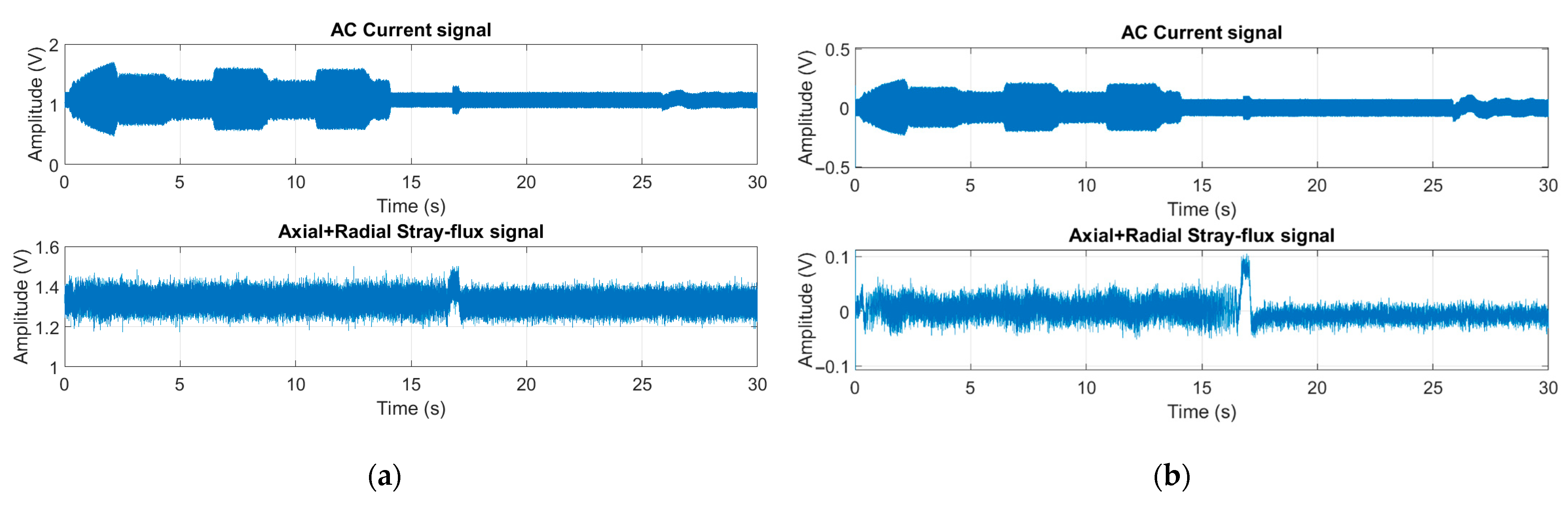
Over the years, several physical properties have been used for the detection and analysis of wear on cutting tools in computer numerical control (CNC) machinery, such as current, vibrations, forces, acoustic emissions (AE), sound and temperature, as well as the use of artificial vision systems, roughness or finish analyses and, recently, the use of magnetic stray flux. Obtaining information on the condition of the tool through machine elements is ideal due to the relationship between the variables measured on the machine and the evolution of wear; in this sense, the spindle motor current is commonly analyzed in motor current signature analyses (MCSA). Zou et al. [3] employed an MCSA to generate an online system from the spindle motor current with a bispectrum signal modulation (BSM) algorithm by identifying the magnitude and phase of the BSM to distinguish between the effects of three levels of wear upon changes in the depth of cut and workpiece diameter of an A3 steel piece, although only one of the obtained features could identify the wear for each depth of cut. On the other hand, Marani et al. [4] implemented a feature extraction of current signals where the root mean square (RMS) values of the tests were obtained and a network with a long short-term memory (LSTM) model was used to predict the evolution of tool wear on a coated carbide tool used for the turning of steel alloy, comparing the accuracy of 30 different architectures to obtain the best suited for the proposed experiment.
Likewise, vibration signals are one of the most exploited measurements for wear detection. Tabaszewski et al. [5] used triaxial accelerometers to distinguish between two tool states at different cutting speeds during turning of EN-GJL-250 with carbide cutting inserts using different intelligent techniques and selecting the most appropriate one, which was a classification and regression tree (CART) with a 2.06% error. Patange et al. [6] used an accelerometer and machine learning (ML) techniques based on trees to classify six types of wear under fixed machining parameters while turning a stainless steel workpiece on a manual lathe; the authors performed a statistical feature extraction, selection and classification, obtaining the best results with a random forest (RF) model, with 92.6% accuracy. In both cases, the placement of the sensor was close to the cutting tool, which is quite invasive of the process.
Regarding the use of force signals, the work of Bombiński et al. [7] shows the use of triaxial sensors placed in the vicinity of the carbide tools employed to cut NC10 steel and 40 HNM steel, which were able to detect accelerated wear using waveform comparison algorithms automatically online based on the operator’s consideration of when the tool life ends during training. As an example of a work using AE and sound, Salodkar [8] placed a sensor on the tool shank and used a fuzzy neural network (FNN) to predict wear online for the machining of En31 alloy steel. Considering the machining parameters used, positive results were achieved for the prediction of seven flank wear states. Casal-Guisande et al. [9] used sound and process variables for risk assessment in the use of two cutting tools for machining aluminum, with favorable results when compared with experts’ opinions, although the methodology requires further validation and optimization.
Another variable used is temperature; in the work presented by Rakkiyannan et al. [10], a sensor was designed and placed on a high-speed steel cutting tool and the changes in temperature and deformation provided information on the state of the tool while cutting mild steel. The results were corroborated with thermographic images, and three levels were successfully detected with a span of 1.2 mm due to the sensor’s degradation. On the other hand, Brili et al. [11] made use of thermographs of a tool within the work area after different durations of cutting to assess whether the tool was in a condition to continue operating. They combined computer vision and deep learning (DL) to obtain a 96% accuracy, identifying the most appropriate time lap for the image acquisition.
Similarly, machine vision and image analysis systems have grown in popularity; in the work presented by Sawangsri et al. [12], a charge-coupled device (CCD) camera was used in the working area to evaluate the progressive wear of the tools when machining SCM440 alloy steel by comparing the number of pixels of the tool before and after being used. The estimations were validated against SMr2 (valley material portion) values measured with a microscope. Bagga et al. [13] employed an artificial neural network (ANN) considering the machining parameters for the turning of AISI 4140 steel and used images captured inside the working area of the carbide tools at specific time intervals. The worn area was obtained by processing the images by filtering, enhancement, thresholding and calculating the number of pixels in the area, and the remaining useful life was determined with two activation functions, sigmoid and rectified linear unit (ReLU), achieving an accuracy of 86.5% and 93.3%, respectively.
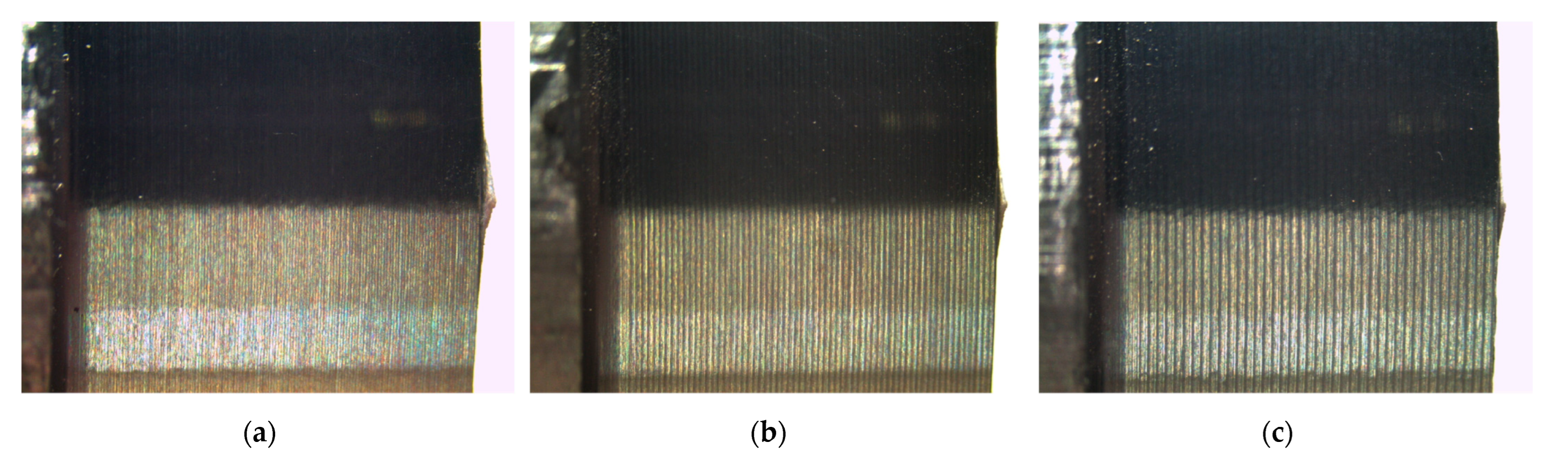
Regarding surface finish analyses, this task can be performed with specialized equipment; however, Shen and Kiow [14] used image analysis of the machined part to extract features and predict tool wear for the turning of AISI 1045 carbon steel using coated carbide inserts with a recurrent neural network (RNN). The surface roughness was predicted with a 92.75% effectiveness from the average gray level value, standard deviation and entropy, and the surface roughness was predicted with 64.59% accuracy.
Likewise, the fusion of information from different sensors to obtain better features has grown in popularity within these systems, allowing the creation of more complex and efficient systems. In this sense, Kou et al. [15] used vibration and current signals to generate RGB images that were combined with infrared images of the tool to distinguish between six levels of wear under variation of the machining parameters using information related to the tool and the machine to train a convolutional neural network (CNN). The method was able to classify the wear with 91% accuracy, but with a longer training time in comparison with other methods and with lower accuracy. Bagga et al. [16] employed force and vibration signals to predict the level of wear in tools with variations in cutting parameters for the turning of EN8 carbon steel using an ANN, and validated this method by comparing the predicted value with the direct measurement of wear for all experiments, obtaining a mean percentage difference of 3.48%.
Kuntoğlu and Sağlam [17] used force, vibration, AE, temperature and current signals to predict tool wear and breakage to design an online monitoring system for the turning of AISI 5140 carbon steel with coated carbide tools. They reported that the ability of temperature and AE to detect wear was 74% effective, and force, AE and vibrations were able to predict breakage. Current had a low contribution to predictions in their experiments. Similarly, the results reported by Hoang et al. [18] indicated the ability of AE and vibrations to predict wear and roughness in the machining of SCM440 steel, combining a Gaussian process regression and adaptive neuro-fuzzy inference system (GPR-ANFIS) algorithms to process RMS values of the signals, achieving an average prediction accuracy of 97.57% in online monitoring with the proposed methodology.
Jaen-Cuellar et al. [19] reported the use of stray flux and current for the detection of three levels of wear with individual variation of two machining parameters for aluminum 6061 turning with coated carbide tools by means of feature extraction, dimensionality reduction and classification with an ANN, achieving a top performance of 94.4%. Diaz-Saldaña et al. [20] employed stray flux signals and image analyses of the surface finish to identify three levels of wear on coated carbide tools with variation in cutting speed in aluminum 6061 turning, obtaining a good differentiation between all the conditions when applying histogram peak counts to the images and feature extraction on the stray flux signals.
It is important to highlight the invasive nature of the sensors for image and sound capture that must be placed in the work area. Temperature, vibration or force sensors must also be placed in the proximity of the cutting tool, an aspect that greatly limits their implementation due to the necessary adaptations to the work area and cutting tasks for an adequate measurement of wear.
On the other hand, the techniques used for processing the information obtained for the identification, evaluation or prediction of cutting tool wear are varied. Several literature reviews have identified the main techniques, tools and trends for processing [21,22,23,24]. Firstly, signals are processed directly in the time domain [3,4,5,6,7,8,9,10,11,12,13,14,15,16,17,18] or techniques or transforms are used for their analyses in the frequency [3,5,18,19,20] or time-frequency [19,20] domains. From here, several techniques are used to obtain features that allow the analysis to be carried out in a better way, such as the use of statistical indicators [3,4,5,6,8,14,18,19,20], time or time-frequency transforms for direct feature extraction [3,4,5,19,20] and, in some cases, methods for the selection of the most appropriate features or dimensionality reduction such as heuristic techniques [5,6,22], linear discriminant analysis (LDA) [19] or principal component analysis (PCA). Subsequently, classification or decision-making techniques tend to use intelligent systems such as different types of neural networks [8,13,14,16,19,25], support vector machines (SVM) [21,22,23,24], hidden Markov models (HMM) [21,22,23,24], fuzzy systems [8,9,17,18] and DL systems [4,11,14,15].
Based on the above, it is possible to note that some of the current research on tool wear makes use of a single variable as the source of information, while others follow the trend towards the use of multiple sensors and the fusion of their information, which in some cases comes from the same source (i.e., part of the machine, tool or workpiece). In both cases, there is a trend towards the use of intelligent systems that allow automatic handling of information for the identification, classification or prediction of tool wear, and process the information in the time and/or frequency domain to obtain characteristics that help to gain a better understanding of the phenomena. The use of intelligent techniques is of great value when processing large amounts of information generated by fused sensors, allowing a more adequate manipulation and interpretation of the data. Another point to note is the implementation of the methodologies, since they can be performed online, allowing process monitoring [3,4,5,7,8,9,10,11,12,14,15,16,17,18,19], or offline once the machining of a part has been carried out [6,13,20,26]. This is an important aspect, since in methodologies that use vision systems or images, the machining process must be stopped for the acquisition of images of the tool or they may be taken after the process; however, this depends on the needs and planning of the process.
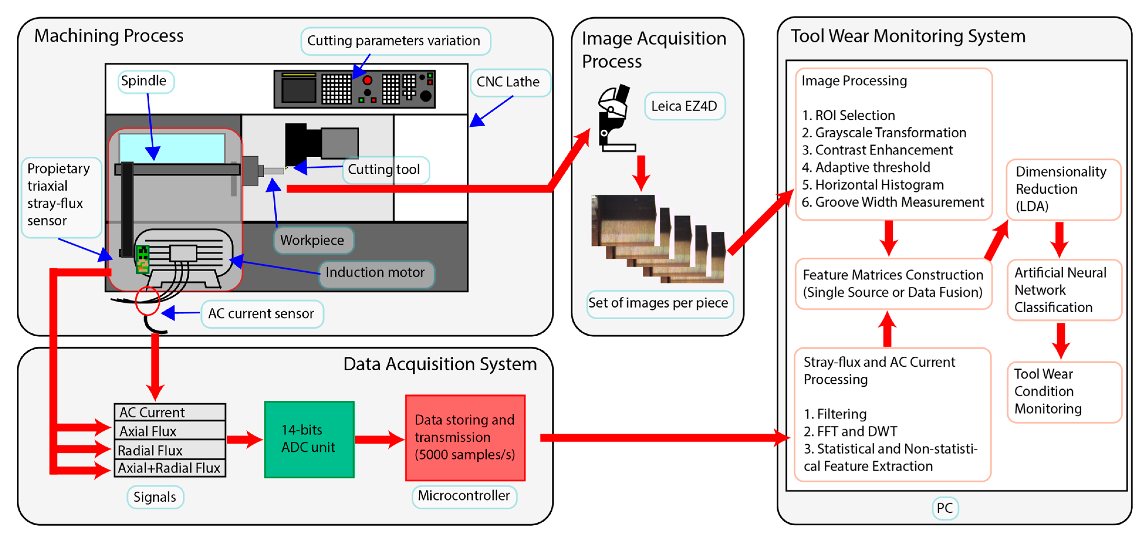
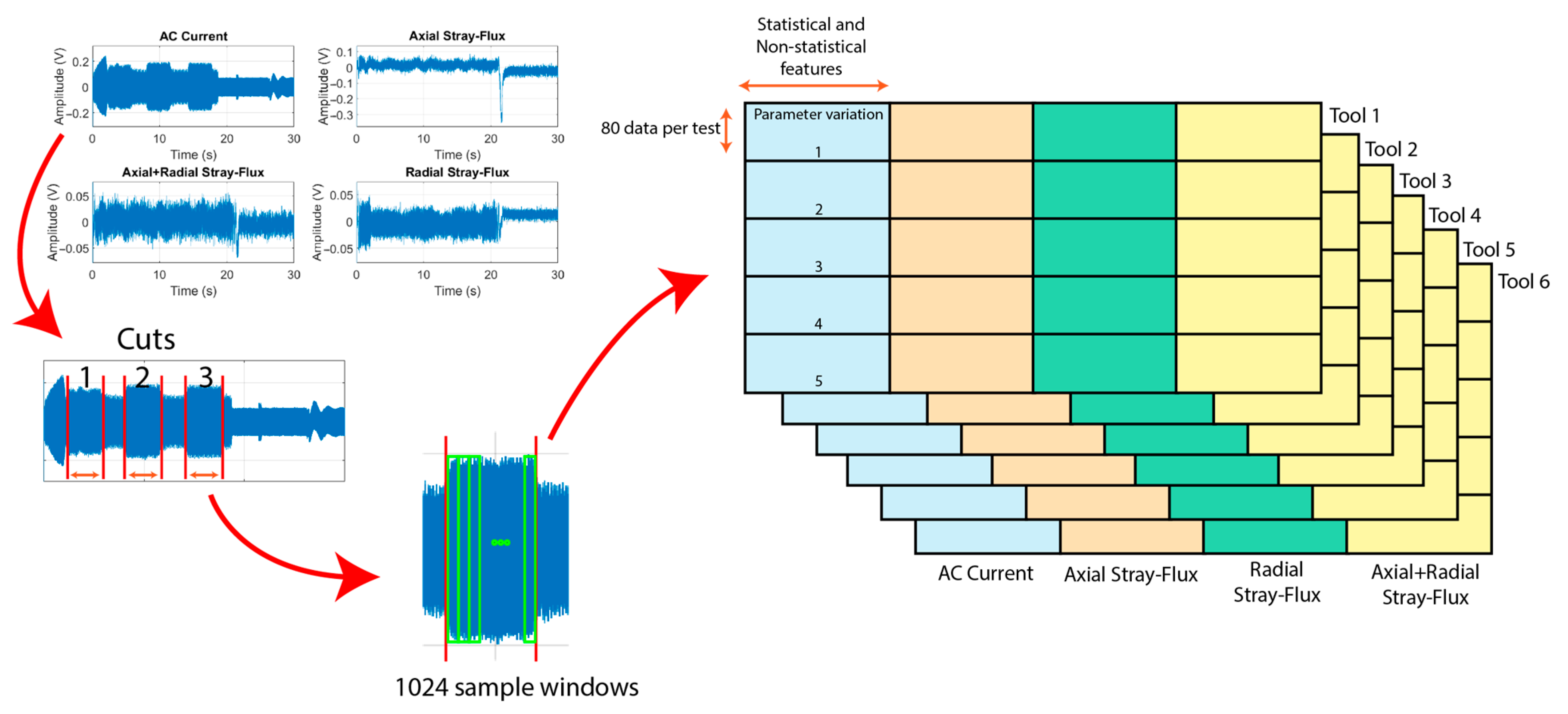
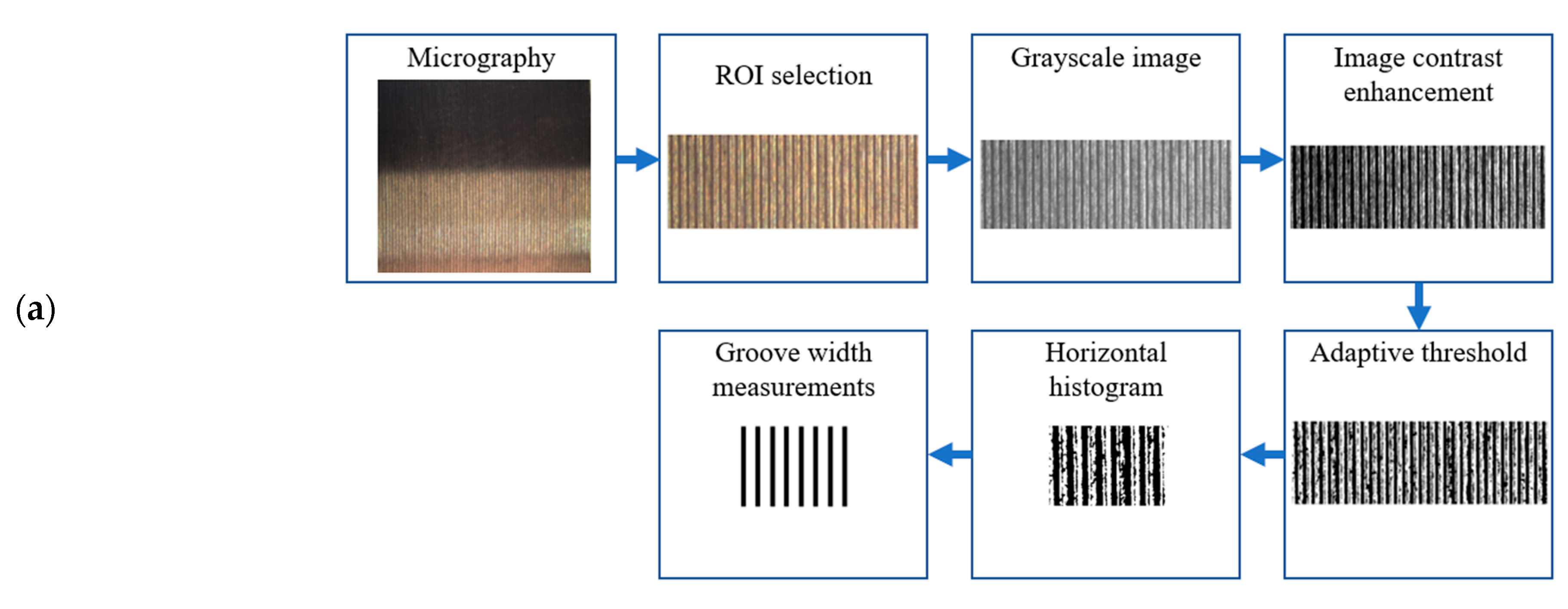
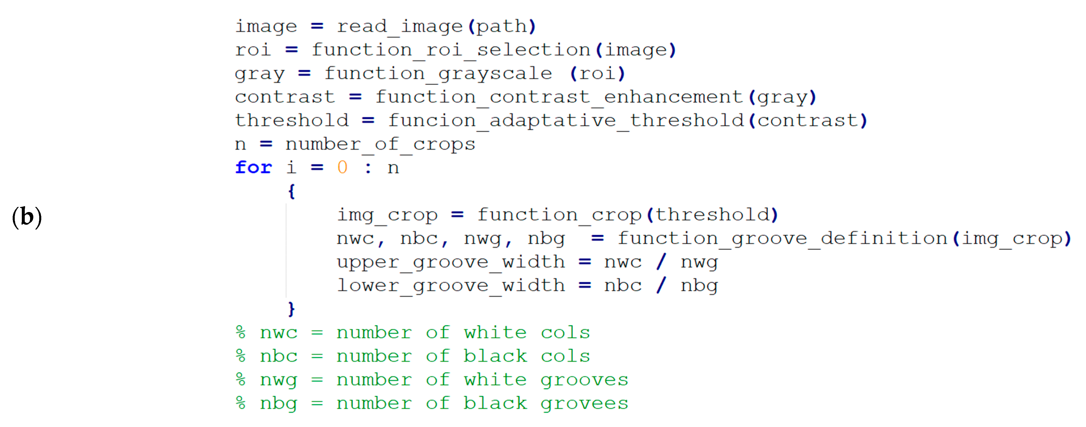
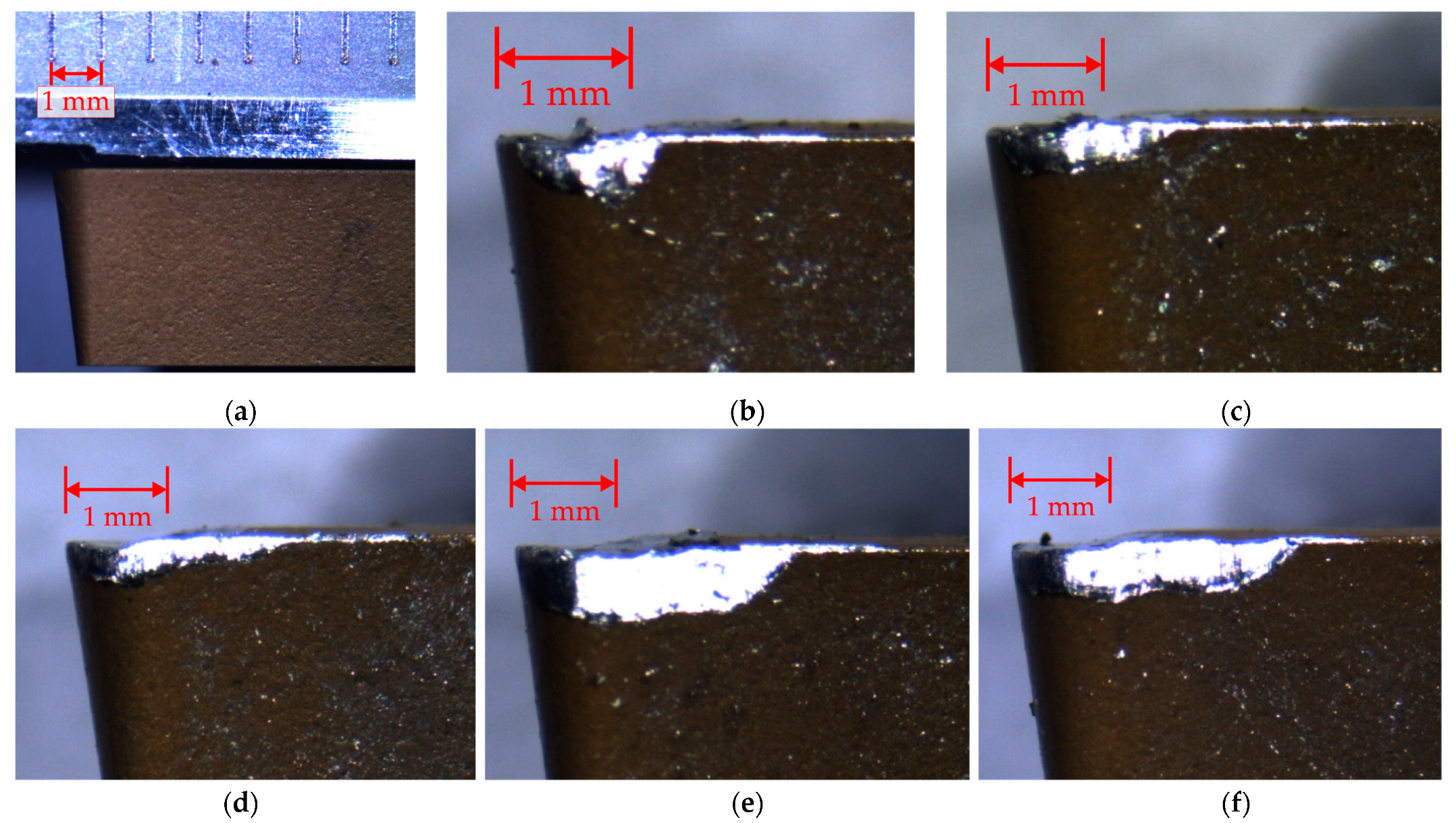
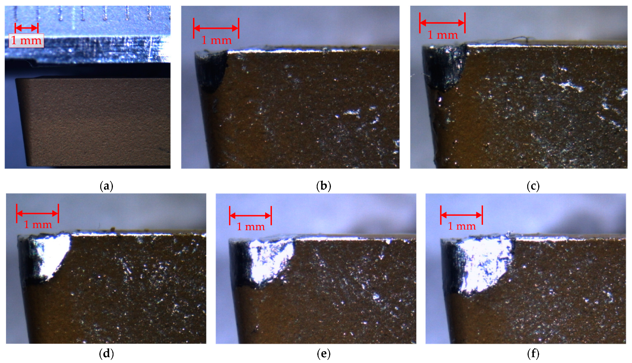
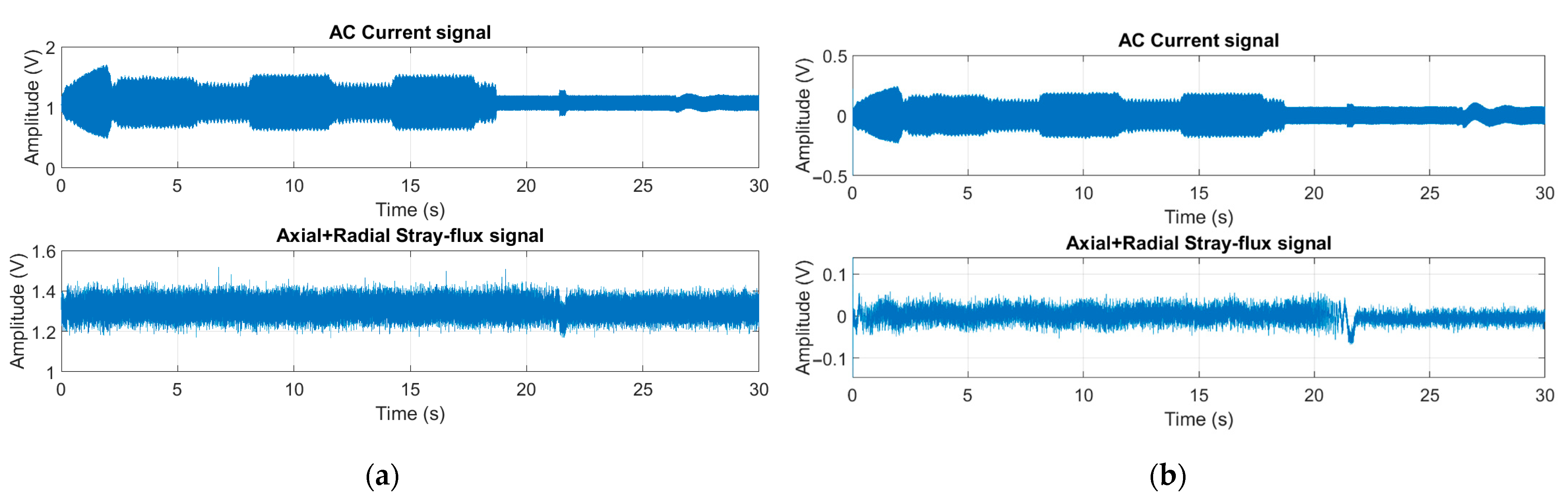
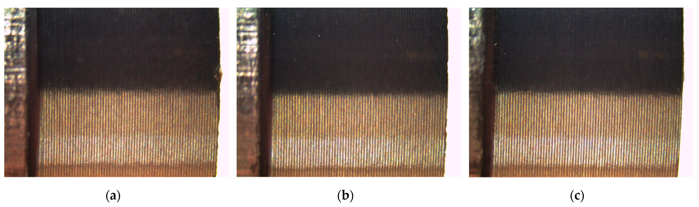
Considering the foregoing, the main contribution of this research is the development of a system for the detection of the level of wear in cutting tools used in a CNC lathe by analyzing the information obtained directly from the spindle motor of the machine using non-invasive current and stray flux sensors, as well as from images of the surface finish of the machined parts. The proposed system allows the analysis of the signals individually and together, allowing it to be adapted to the user’s needs to evaluate the wear online or after the process is finished, all through the use of the fast Fourier transform (FFT), the discrete wavelet transform (DWT), statistical and non-statistical indicators, dimensionality reduction by linear discriminant analysis (LDA) and a feed-forward neural network (FFNN) for wear classification under the individual variations of the cutting speed and the feed rate of the tool.
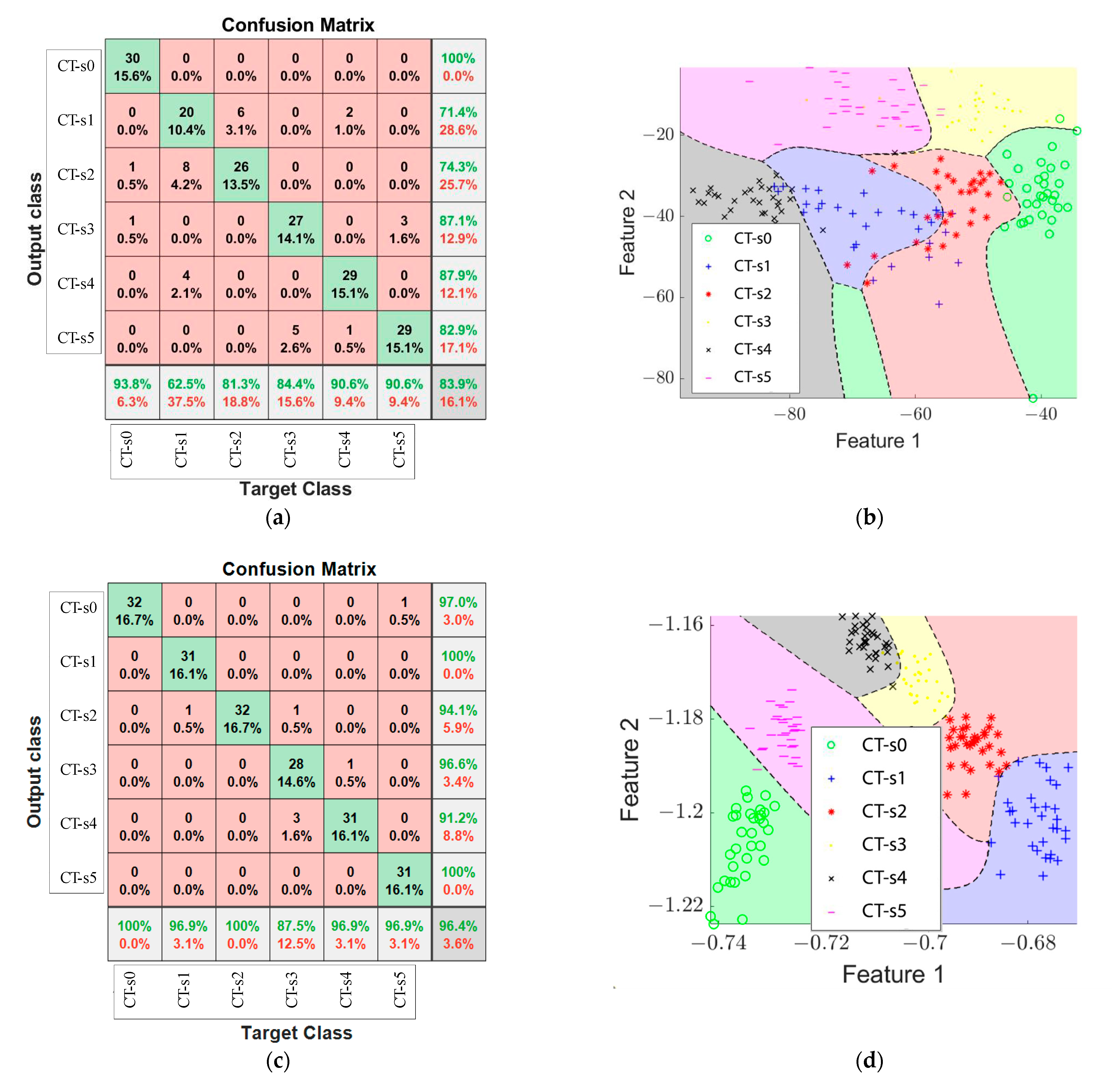
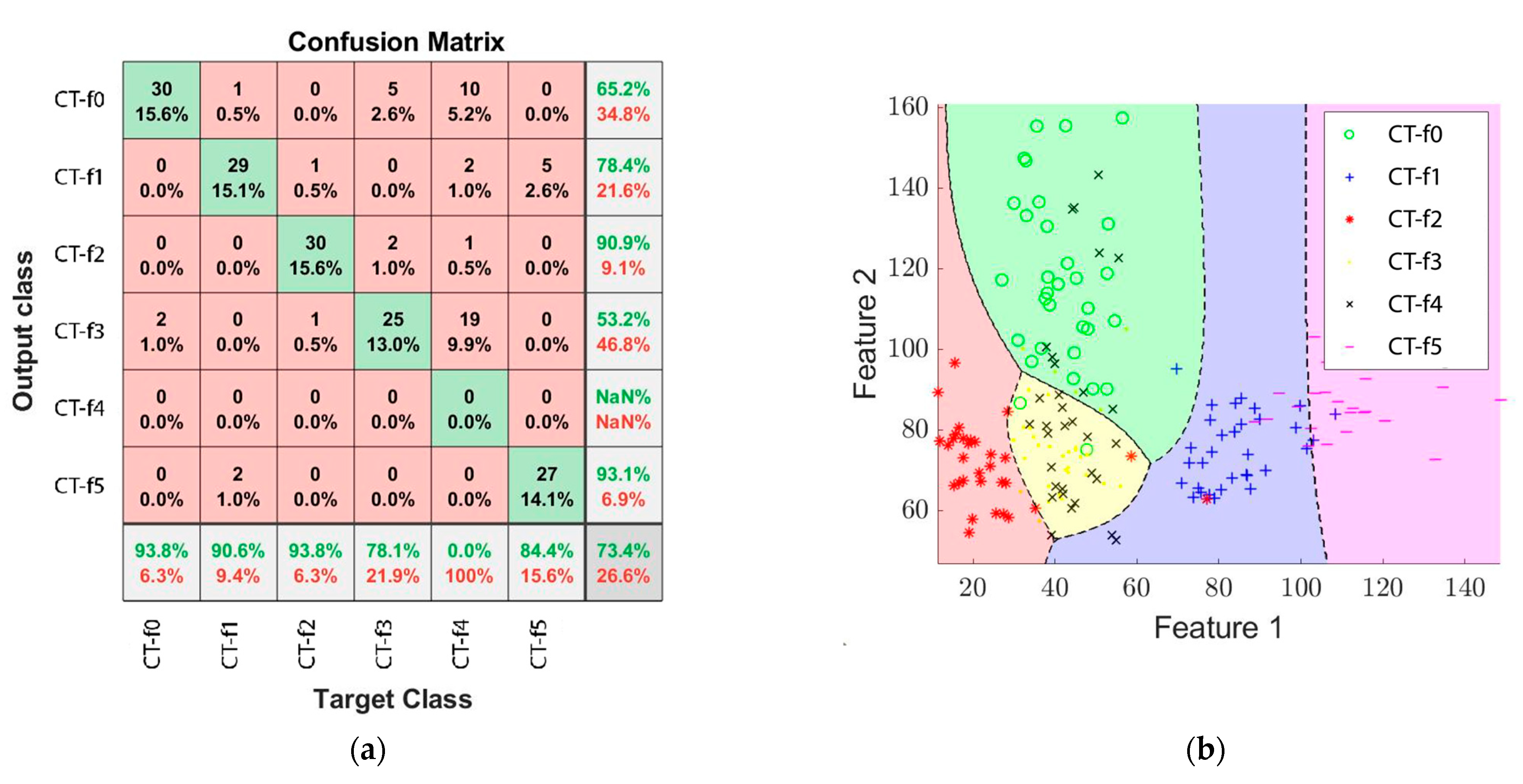
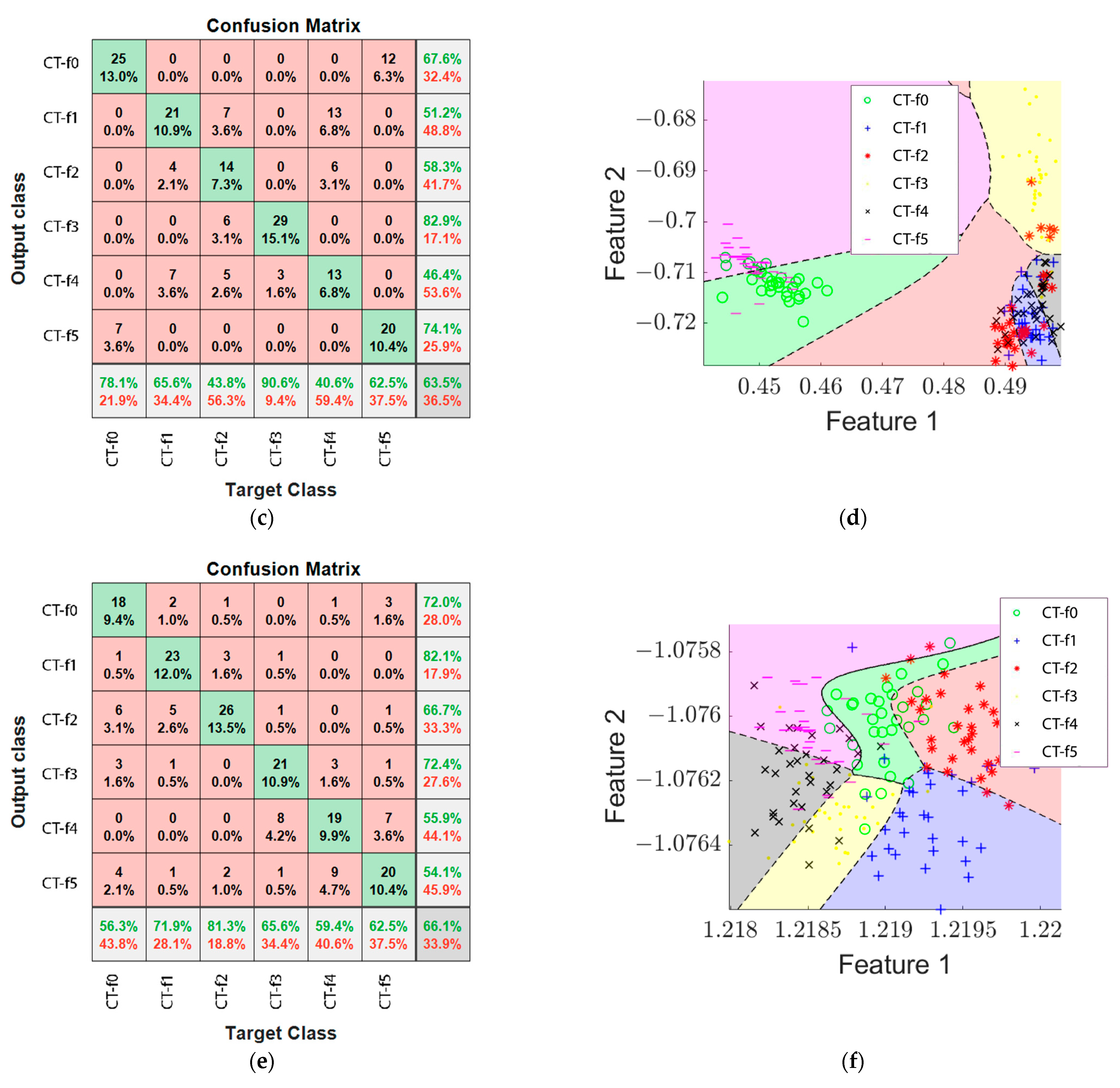
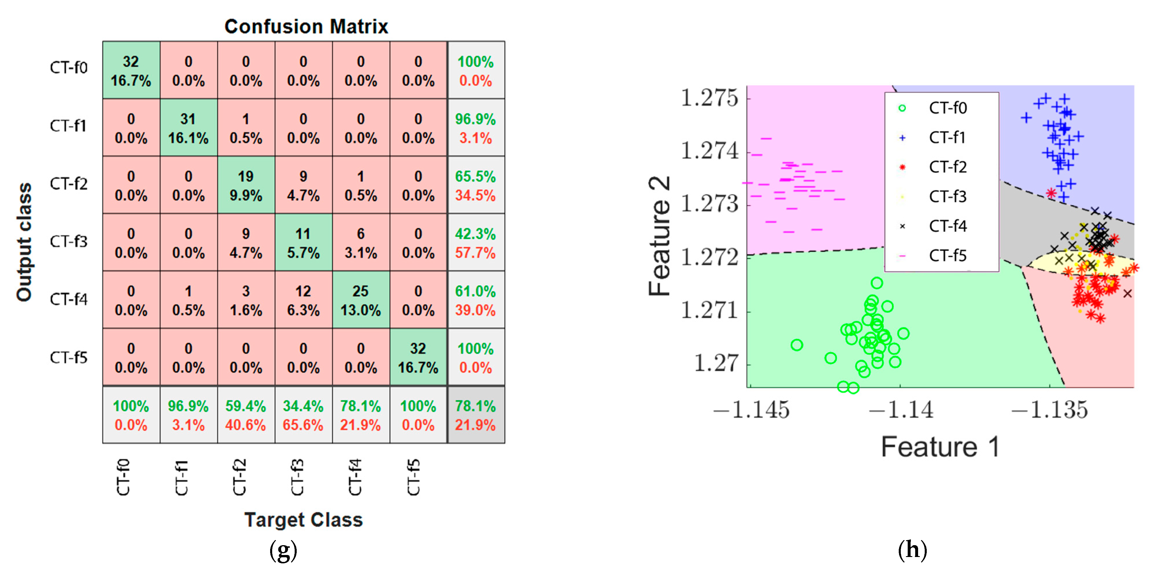
2. Theoretical Background

2.1. CNC Lathe and Machining Parameters

The lathe is considered the oldest machine tool, which makes it simple and versatile, and it is used to produce round shapes through operations such as turning, facing or boring [27]. There are different types of lathes, most of them are manually controlled or slightly automated, in addition to computer numerical control (CNC) lathes, where a computer allows a faster and more precise control of operations, allowing the reliable production of higher quality parts with high dimensional accuracy, provided that the tools used are in good condition.
Within the turning process there are several parameters that have an impact on the development of operations and the wear that the tool will suffer in the process. These parameters depend on the materials of the workpiece and the tool to be used; a correct selection of parameters is essential to avoid tool fractures, accelerated wear and high temperatures or vibrations that can greatly affect the production and the machine. There are tables that provide appropriate working ranges for different materials, such as those presented in [27].
The three most important parameters for machining operations are the depth of cut (d), cutting speed (V) and tool feed rate (f). The depth of cut is the average between the initial diameter of the workpiece (Do) and its final diameter (Df), as shown in (1); the cutting speed is the superficial (tangential) speed of the workpiece, in m/min, as a function of Do and the spindle speed (N) in rpm, as shown in (2); and the tool feed rate is the distance the tool travels in one rotation of the spindle, in mm/rev, and can be defined by the linear feed rate of the tool through the workpiece (vf) and N, as defined in (3).
d = D 0 + D f 2
V = π D o N
f = v f N

2.2. Image Processing

Image processing is a powerful tool for the development of condition monitoring systems, allowing good analysis and detection of different conditions or faults in the processes where it is implemented; however, the results greatly depend on the processing applied to the information acquired, which includes techniques such as grayscale conversion, contrast enhancement, adaptive thresholding and histograms.

2.2.1. Gray Scale Images

A grayscale image represents only the value of light intensity, where, generally, the range of each pixel is between 0 and 255; that is, there are a total of 256 gray levels [28]. Equation (4) is used to obtain such an image, where Igray represents the pixel in gray level and r, g and b are the red, green and blue components of each pixel of the color image, respectively.
I g r a y = 0.299 r + 0.587 g + 0.114 b

2.2.2. Image Contrast Enhancement

The Gamma transform is a nonlinear transform that is typically used for luminance or color coding or decoding of images for electronic display and acquisition devices [29]. This transform is defined in Equation (5), where y is the output gray level, c is the constant to normalize the pixel value to the range of interest, x is the input gray level and γ is the gamma value. When γ < 1, lightening effects are produced in the image; conversely, when γ > 1, darkening effects are produced.
y = c x 1 γ

2.2.3. Adaptive Threshold

In computer vision systems, thresholding seeks to classify the pixels of an image as “light” or “dark” based on a given value. Adaptive thresholding is based on an algorithm in which each pixel is compared to the average intensity value of the surrounding pixels, as established in [30].

2.2.4. Horizontal Histogram

A histogram of an image I is a vector that shows the frequency with which each of the gray levels of an image appear, included in the range of the minimum and maximum gray levels [29]. Similarly, a horizontal histogram (histj) of a binary image (bin(i, j)) represents the number of pixels that appear as white in each of the columns (w) of the image width, using Equation (6).
hist j = i = 0 h 1 bin ( i , j )       for   j   =   0 ,   1 ,   ... ,   w 1

2.3. Stray Flux Signal and AC Current Analysis

Stay flux is an effect or secondary characteristic present in windings and has been studied for a long time [31], becoming an important physical quantity for the study of faults in electrical machines in recent years. Stray flux applications for the monitoring of electric motors are based on the property that any fault or modification in its state is reflected in changes in the magnetic field of the machine [32].
A stray flux analysis is carried out by analyzing two components: the axial component, whose plane includes the machine axis, generated by the current at the end of the stator windings or the ring at the end of the rotor cage; and a radial component, which is perpendicular to the machine axis and is due to the air gap flux escaping from the machine after the attenuation of the stator and the machine casing. These components can be measured by placing sensors in certain positions. Figure 1 shows common positions of coil sensors for stray flux signal acquisition from the radial plane in Figure 1a and from the axial plane in Figure 1b. Pos.3 allows the measurement of the radial stray flux component, Pos.2 allows the measurement of the axial stray flux and Pos. 1 allows the measurement of a mixture of the radial and axial stray flux.
In this development, a proprietary triaxial stray flux sensor [33] is used, shown in Figure 2. This board allows capturing signals from the three orthogonal magnetic stray flux components.
On the other hand, and as mentioned in the Introduction, a current analysis is a commonly used technique for wear detection [22] because the current demand of the machine’s spindle motor is related to the changes that occur in the machining operations, allowing identification of the progression of wear suffered by the cutting tool.

2.4. Intelligent Tools and Sensor Fusion

2.4.1. Sensor Fusion

According to [22], signal fusion in tool condition monitoring systems occurs in three different levels: the first one corresponds to the signals as they were acquired by the sensors to be subsequently conditioned and processed, which is a little used methodology; the second level is the fusion of the features obtained from the analysis of each of the acquired signals, allowing to generate a set of features that provide the most relevant information of the phenomenon for the generation of models, which is the most used methodology; and the third option is the fusion of the models generated for each of the signals in order to create a more robust system that provides a better decision than the classifiers individually.

2.4.2. Statistical Features

Statistical indicators are commonly used tools within the field of tool condition monitoring since they allow obtaining useful information that reflects the state of wear without the need for a high computational load. They are employed in some methodologies directly for wear identification and in others as a way of obtaining characteristics, some of the most common being the average value, RMS, variance, standard deviation, skewness and kurtosis [24]. Likewise, they have been widely used within fault identification in electromechanical systems; thus, a set of 15 indicators (Equations (7)–(21)) that have shown satisfactory results in the literature [34] have been considered and are listed in Table 1.

2.4.3. Non-Statistical Features

There are indicators based on non-statistical characteristics that allow to obtain information that describes the behavior of the information through the analysis of relationships or qualities present in the data, some of them being fractal dimension, DWT energy, Shannon entropy (H) and wavelet entropy (Sw).
Fractal dimension. Fractals are geometric shapes such that when subdivided into parts, each part is a smaller approximate copy of the original. This quantity is used as an indicator of how much a fractal fills a space as it approaches smaller and smaller scales [35] or as a measure of self-similarity or the appearance of patterns in signals within the time domain [36]. There are several algorithms for its calculation, with results ranging from 1.0 for straight lines to 2.0 for a plane. Considering this, two formulations were used for this research, Higuchi’s fractal dimension (HFD) and Katz’s fractal dimension (KFD), whose calculation procedures are described below.
Higuchi’s fractal dimension (HFD). The procedure for HFD calculation consists of four steps [37]:
  • The original signal in the time domain, X, containing N samples is decomposed into a new series or sequence in the same domain, x k m , using (22), where m and k are integers corresponding to the initial time and the time interval, respectively, while the term in square brackets denotes the rounding performed to the integral part of the calculated value.
x k m = x m ,   x m + k , x m + 2 k , , x m + N m k k               m = 1 , 2 , , k
2.
For each sequence of x k m calculated, the average normalized length, Lm, is obtained using (23), which uses the factor [(N − m)/k] as a normalizing factor.
L m k = N 1 k N m k i N m k x m + i k x m + i 1 k
3.
Using Equation (24), the total length, L(k), is obtained for a given value of k.
L k = m = 1 k L m k
4.
The value k is modified such that k = k + 1, and as long as k < kmax, steps 1 to 3 are repeated. kmax is a selected value for which the slope of the line of best fit to the plotted diagram in the plane (ln[L(k)] versus ln [1/k]) remains constant. The slope of this line represents the fractality value, HFD, of the analyzed signal.
Katz’s fractal dimension (KFD). The algorithm to obtain KFD consists of three steps [38]:
  • Starting from the signal, X, with N samples, the maximum Euclidean distance, d, between the first sample, x1, and a sample xk, equal to k = 1, ..., N, is obtained.
  • The arithmetic sum of the Euclidean distances, L, between consecutive samples of the signal X is obtained with (25) and its average, a, is obtained using (26).
L = k = 2 N d i s t x k x k 1
a = L N 1
3.
KFD is calculated using Equation (27).
K F D = log L / a log d / a
DWT energy (γDWT). The DWT energy parameter, γDWT, is a normalized indicator defined as the inverse ratio between the energy of a signal decomposition after the use of DWT and the energy of the original signal in a time window, delivering a result in decibels (dB) [39]. Equation (28) shows the mathematical expression for its calculation, where emfj is the value of the j-th sample of the original signal, emf; di(j) is the j-th point of the selected wavelet signal and Nb and Ns are the start and end sample of the interval of interest, respectively.
γ D W T d B = 10 log j = N b N s e m f j 2 j = N b N s d i j 2
Shannon entropy (H). Claude Shannon [40] introduced this concept as a measure of the uncertainty of an information source, as well as of the noise or disorder of a system, relating it to the uncertainty that exists in an experiment or in a random signal. Equation (29) shows the definition of this parameter, H, for a signal x with possible values xi with a probability of occurrence of p(xi).
H X = i p x i log p x i
Wavelet entropy (Sw). This indicator, Sw, is a measure of the degree of order/disorder present in a wavelet signal and provides information associated with the dynamic processes related to the source of the original signal [41]. To obtain Sw, it is necessary to calculate the energy of the i-th wavelet decomposition levels, Ei (30), and the total energy of the whole decomposition, Etot (31). With this it is possible to obtain the normalized wavelet energy, pi, as shown in (32), and to finally use Equation (33), where m and n are the first and last decomposition level of the signal, respectively.
E i = k C i k 2
E t o t = i E i
p i = E i E t o t
S W S W p = j = m n ln p i

2.4.4. Linear Discriminant Analysis (LDA)

LDA is a supervised dimensionality reduction technique used when there is prior knowledge about the classes within the dataset. This technique searches for linear combinations between variables to maximize the between-class scatter matrix (Sb) and make them as far apart as possible while minimizing the within-class scatter matrix (Sw) to compact the data as much as possible [42]. The procedures for calculating Sb and Sw are shown in Equations (34) and (35), where the dimension k of the subspace is defined as k = C − 1, where C is the number of classes, mk is the mean of class Ck, m is the global mean, nk is the number of samples and xi is the i-th sample of class Ck.
S b = k n k m k m m k m T
S w = k i C k x i m k x i m k T
Subsequently, the GLDA subspace is obtained by using Equation (36), whose solution is given by the k eigenvectors of Sw−1Sb associated with the highest eigenvalues.
G L D A = m a x T r U G T S b G G T S w G = g 1 ,   ,   g k
To obtain the data transformed to the new space, Y, a projection of the original data, X, is made in the generated subspace, as shown in Equation (37).
Y = G L D A T X

2.4.5. Feed-Forward Neural Networks (FFNN)

Artificial neural networks (ANNs) are tools within the field of artificial intelligence (AI) that seek to recreate the functioning of the human brain by mimicking the neural interconnections in the brain in order to create intelligent systems capable of performing complex learning to extract patterns and recognize trends from complex data structures [43]. ANNs are composed of three layers of nodes, called neurons, which perform operations with the data entered in the input layer, passing through a hidden layer where a nonlinear transformation of the information is performed to obtain a classification of the data in the output layer. When a network topology is configured so that the outputs from one layer are fed into the next one, it is called a feed-forward neural network (FFNN), and this is the most common configuration [44]. Additionally, ANNs can have more than one hidden layer, becoming deep neural networks (DNN), where the topology to be used is decided by empirical issues related to the applications in which they are used [45].

3. Materials and Methods

3.1. Materials and Experimental Setup

The experiments were carried out on a DYNAMACH CNC lathe, shown in Figure 3a, with Fanuc Oi Mate-TC control, a 3-phase induction motor with 4 poles and a rated power of 3.7 kW powered by a variable frequency drive (VFD) at 220 Vac. The components that make up the data acquisition system (DAS) are shown in Figure 2 and Figure 3b. A proprietary triaxial system, shown in Figure 2, using Allegro Microsystems A1325 Hall effect linear sensors, which have a sensibility of 3.125 mV/G, an ambient temperature range between −40 °C and 150 °C and an internal bandwidth of 17 kHz (−3 dB), and are positioned to measure the orthogonal magnetic stray flux components (axial, radial and axial + radial stray flux), was used for the stray flux signal measurement. A Fluke i3000s Flex-24 Rogowski-type AC current clamp was used to measure the current signal, which has three current ranges of 30, 300 and 3000 A, output sensibilities of 100, 10 and 1 mV for the respective current ranges and a bandwidth from 10 Hz to 50 kHz. The capture and transmission of the stray flux and current signals were executed with a Texas Instruments microcontroller that has a 14-bit analog-to-digital converter (ADC) working at a sampling frequency (fs) of 5000 samples per second for a more adequate sampling of the signals. The placement of the DAS and PC, as well as the location of the spindle motor and the work area of the CNC lathe, can be seen in Figure 3b, with a close-up view of the placement of the stray flux sensors in Figure 3a. With this it is possible to observe the non-invasive placement of the measurement equipment for the process.
The experiments were performed using BOEHLERIT TCMT-16T308-MP LCP-25T triangular coated cutting tools, using a total of 12 cutting tools divided into two groups, one for each machining parameter (cutting speed and tool feed rate), with a total of six states: a new state and five levels of progressive wear. The insert sides were 16.5 mm long and 3.97 mm tall with a corner radius of 8 mm and ISO class-P with a toughness of 25 according to ISO, as stated in the manufacturer’s catalog. The workpieces were 6061 aluminum bars with a diameter of 1.5 in and the chemical composition of this alloy is show in Table 2. It has an ultimate tensile strength between 125 and 310 MPa, a yield strength ranging from 55 to 275 MPa, depending of its temper, and a Young’s Module of 69 GPa [27]. Figure 4 shows some of the specimens produced during the experiments, where Figure 4a,b shows the no wear and mayor wear tools machined during the cutting speed test, respectively, while Figure 4c,d shows the tools with no wear and the one presenting with the greatest wear in that set machined for the feed rate test.
For the capture of the micrographs of the machined parts, both a LEICA EZ4D microscope and LAZ EZ software were used; likewise, these instruments were used to capture micrographs of the cutting tools used in order to obtain a wear area for each one as a validation tool for wear classification.

3.2. Proposed Methodology

This section presents the methodology applied for the development of this research. Figure 5 shows the methodological diagram, which consists of four main blocks: the machining process, the data acquisition system for current and stray flux signals, the image acquisition process of the machined parts and the tool wear monitoring system.
The machining process block considers the CNC lathe, the workpiece material, the cutting tools and the machining parameters used for the experimental tests, as well as the placement of the stray flux and current sensors on the spindle motor for data acquisition. In this part, the workpieces were fabricated considering the recommended cutting parameter ranges presented in [27] for the machining of aluminum 6061. The machining operations performed were turning and making three cuts along the piece, lasting 30 s per workpiece.
The data acquisition system block describes the use of the proprietary triaxial stray flux sensor and a current sensor placed on the spindle motor to capture the corresponding signals and the use of a 14-bit ADC integrated to a commercial microcontroller to capture the data. For each of the experiments, the AC current and the axial, radial and axial + radial stray flux signals of 30 s length were captured with the DAS, each one having a total of 150,000 samples considering the fs specified above.
For the image acquisition block, a commercial microscope was used to capture a series of images for each workpiece in order to increase the amount of information available for analysis. The images obtained with the LEICA EZ4D microscope were in RGB format, with a resolution of 2048 × 1536 pixels. Incident and oblique illumination was carried out in a portion of the part height by means of the seven LEDs of the device. For each workpiece, the illuminated area corresponded to one-twelfth of the perimeter, which allowed the capturing of 12 images per bar. As there were five variations of each machining parameter and six levels of tool wear, a total of 360 images were acquired for the cutting speed case and another 360 were captured for the tool feed rate test. The images were stored in a PC for later analysis.
Finally, the tool wear monitoring system block describes the processing stages of the information acquired for the development of the wear monitoring system from the individual or fused use of the information sources. For the stray flux and current signals, a preprocessing and conditioning are performed; first, a digital filtering of the signals was carried out due to the presence of noise with a Butterworth filter of order 10 and the offset present due to the characteristics of the sensors used was eliminated. The next stage was preprocessing using the FFT [47] to obtain the fundamental frequency component present in the signals because the motor is fed with a VFD. Once the fundamental frequency of the signals was obtained, the DWT [48] was used to decompose the signals into ten levels with the Daubechies44 mother wavelet [49] and the fundamental frequency was used to identify the most appropriate reconstruction level to obtain information. With the reconstructed signals, the statistical and non-statistical indicators were calculated using Equations (7)–(21) and Equations (22)–(33), obtaining 20 indicators or characteristics for each of the acquired signals, with which matrices of characteristics were generated. For the generation of these matrices, the procedure illustrated in Figure 6 was followed, where for each of the signals, the three cuts made with the tool were identified. Subsequently, fixed-size 1024 sample windows were used for the calculation of the indicators, giving a total of 80 windows for each signal and 20 indicators for each window and thus creating an 80 × 20 feature matrix for each of the signals per experiment. This process was repeated for each sensor signal captured for the 30 experiments conducted for the five variations of each machining parameter with their six corresponding tool wear levels.
For the analysis of images of the workpieces, the procedure shown in Figure 7a was followed for each of the images captured of the machined surface for each test conducted. First, for each image, the region of interest (ROI) to be analyzed was selected, which was the illuminated area of the original image. Second, the color image was converted to grayscale through Equation (4). Third, the contrast of the image was enhanced through a gamma transformation (Equation (5)), automated to adapt the enhancement to the illumination characteristics present in each image. Fourth, the optimal threshold level was obtained through an adaptive thresholding; then, with this obtained value, the image was binarized with the objective of dividing the lower groove in black and the upper groove in white. Fifth, the image was cut to obtain 80 subdivisions for each test of both speed and wear. At this point, it is important to mention that 12 images were taken for each test. Sixth, for each subdivision carried out, a horizontal histogram was obtained (by column). If there was a greater predominance of black tones, it was taken as the lower groove; on the contrary, if there was a greater predominance of white tones, it was taken as the upper groove. Depending on the result, the column was set to white or black. Finally, to obtain the width of the upper and lower grooves, the number of columns across the width of both the upper grooves (white tones) and the lower grooves (black tones) was added individually and divided by the number of upper and lower grooves, respectively. This process was automated, following the pseudocode in Figure 7b, to allow a better integration to the tool condition monitoring system developed.
With the features obtained from the current and stray flux signals, as well as from the images, we proceeded to the dimensionality reduction of the feature matrices for the analyzed sources, individually and fused, using LDA to generate 2D representations and compacting the information for better interpretation and analysis. With the reduced indicator matrices, an FFNN with an architecture of two input neurons and two hidden layers with four and six neurons, respectively, was used for the classification of the wear conditions of the tools used. This procedure was carried out for each of the machining parameters that were varied for testing, i.e., cutting speed and tool feed rate.

3.3. Case Studies

In the reported literature, the majority of studies vary the cutting parameters to select the most adequate combination to extend the useful life of the cutting tools; however, the focus of this research is on the correct detection of wear in two case studies. In the first case study, the cutting speed was varied while the rest of the parameters were constant. In the second case study, the tool feed rate was varied, keeping the other parameters fixed. In order to define the parameters to be used, the ranges recommended in [27] for the machining of 6061 aluminum were consulted.

3.3.1. Case Study 1: Cutting Speed

For the cutting speed tests, a matrix was designed with the cutting parameters to be used, which are shown in Table 3. As mentioned before, the cutting speed (V) varies while the depth of cut (d) and feed rate (f) remain constant, with five different speeds used to carry out these experiments.
Figure 8 shows images of the cutting tools used for these experiments, obtained using a Leica EZ4D microscope and dedicated software. Figure 8a shows the scale reference for the measuring using a Vernier, while Figure 8b–f presents the same scale reference with a magnified view of the wear area of the inserts. For these tools, the wear areas (Af) measured for validation purposes are as follows: CT-s0′s Af = 0.0 mm2, CT-s1′s Af = 0.467 mm2, CT-s2′s Af = 0.5858 mm2, CT-s3′s Af = 0.7057 mm2, CT-s4′s Af = 1.7016 mm2 and CT-s5′s Af = 1.739 mm2. With the five variations of the machining parameters in Table 3 and the six available tools, thirty experiments were performed.

3.3.2. Case Study 2: Tool Feed Rate

For the tool feed rate tests, a matrix was designed with the machining parameters to be used, which are shown in Table 4. In this case, five variations of the tool feed rate (f) were considered while the depth of cut (d) and cutting speed (V) were kept constant.
Figure 9 shows images of the cutting tools used in this case study, obtained using a Leica EZ4D microscope and dedicated software. As for the previous case study, Figure 9a shows the scale reference for the measuring using a Vernier, while Figure 9b–f presents the same scale reference with a magnified view of the wear area of the inserts. For these tools, the wear areas (Af) measured for validation purposes are as follows: CT-f0′s Af = 0.0 mm2, CT-f1′s Af = 0.5471 mm2, CT-f2′s Af = 0.8729 mm2, CT-f3′s Af = 1.2645 mm2, CT-f4′s Af = 1.7377 mm2 and CT-f5′s Af = 2.2814 mm2. With the five variations of the machining parameters in Table 4 and the six available tools, thirty experiments were performed.

4. Results

This section details the results of the tests performed for the case studies specified applying the proposed methodology. During the analysis and processing of the information, it was found that the stray flux signal of combined axial and radial components provided higher quality information, so the analysis focused on using only that stray flux signal along with the current signal.

4.1. Results of Cutting Speed Variation Tests

As mentioned in the methodology, the signals obtained from the current and magnetic stray flux sensors required a filtering and conditioning stage for the elimination of noise present in the signals and the offset of the sensors. Figure 10 presents the analyzed signals corresponding to the test with a cutting speed of 100 m/rev with the CT-s5 tool, which had highest wear of the batch. Figure 10a shows the signals captured before conditioning and Figure 10b shows the conditioned signals after digital filtering with the Butterworth filter of order 10 and after offset elimination. The change in the signals after preprocessing is clear, especially the change in amplitudes because of the noise. This filter allowed a good high frequency noise elimination without affecting the signal amplitude, as the frequencies related to the machining process are of a lower range [27]. Once the signals were conditioned, the process described in Figure 6 was implemented to obtain the feature matrices for each signal. First, the cuts made by the tool were identified and then 1024 data windows were used to calculate the features from the cuts in the signals, creating an 80 × 20 feature matrix for each signal. The process was repeated for all signals.
Nowadays, one of the most commonly used techniques for the measurement of objects in images is the pixel counting technique (PCT), since it has the advantage of having low measurement errors [50,51]. This technique is based on counting the number of pixels existing in a reference unit at a certain distance between the target and the camera. Subsequently, based on this, a relationship between the number of pixels and the measurement of an object can be obtained. Previous research has shown the effectiveness of thresholding for the segmentation of regions of interest (ROIs) [52,53,54]. For the proposed method, different experiments were performed to have a robust methodology to segment the grooves (lower and upper) in order to obtain the width measurement. The techniques tested were for contrast enhancement and thresholding. It is important to mention that for the reference measurement, PCT was used. For 1 mm there were 135 pixels. Table 5 shows the results obtained for speed tests (using the CT-s4 insert with Af = 1.7016 mm2 at a cutting speed of 70 m/rev). For this case, the lower groove was 7 pixels (0.0518 mm) and the upper groove was 15 pixels (0.1111 mm) measured with the PCT.
Photographs taken of the parts machined with the CT-s5 tool at 60 m/rev, 80 m/rev and 100 m/rev are shown in Figure 11a, Figure 11b and Figure 11c, respectively. To the naked eye, the differences in the grooves made by the tool between these images are minimal. For each one of the images captured, the process described in Figure 7 was applied, producing a matrix with the groove characteristics for each experiment conducted.
Once the feature matrices were produced for each experiment and signal, an FFNN was trained and tested to assess the capabilities of the proposed methodology. The results of the effectiveness of wear classification with the FFNN for each of the machining conditions considered are shown in Table 6, grouped according to the source of information analyzed, as well as the average effectiveness value for each of them. It is possible to observe that each of the individual sources obtains a certain percentage of effectiveness. Using the current as the source presents the lowest average effectiveness at 73.02%, followed by the analysis of images, which presents an average of 77.5%, while the use of the combined axial + radial stray flux signal generated the best average accuracy of 89.78%. Likewise, when the information is fused, considerable increases in efficiency were obtained. Using a fusion of images and current presented the lowest effectiveness of the combined methods, at 84.48%, followed by the fusion of current and stray flux at 92.3%, while the fusion of images, current and stray flux reached a 94.06% effectiveness, 0.8% lower than the effectiveness of the fusion of images and stray flux, at 95.02%.
In Figure 12, some results are shown for comparison considering the experiments at 100 m/rev. The confusion matrix for the image analysis is shown in Figure 12a, while the classification performed by the FFNN can be seen in Figure 12b, showing how the analysis of the surface finish gives a good separation between the classes with little overlap for all tool conditions. The confusion matrix for the stray flux analysis is shown in Figure 12c and the classification is shown in Figure 12d, exhibiting a nearly perfect segregation of the data with almost no misclassification on the wear conditions. The confusion matrix for the current analysis is displayed in Figure 12e and the classification is shown in Figure 12f, exhibiting the inability to correctly identify the tool wear in comparison to the other two signals with a clear separation of the tool with no wear and overlaps for the other tool conditions. The confusion matrix for the fusion of the three signals is shown in Figure 12g and its classification is shown in Figure 12h. It is possible to observe a small performance enhancement in the classification, with minor overlap between the classes corresponding to Af = 0.467 mm2 and CT-s2′s Af = 0.5858 mm2. These graphics show the main advantage of sensor data fusion; the increase in data leads to a more robust system with a better performance.

4.2. Results of Feed Rate Variation Tests

As for the cutting speed tests, the stray flux and current signals were filtered using a Butterworth filter of order 10 and the sensor offset was subtracted. After the signals were preprocessed, the process for the calculation of the feature matrixes in Figure 6 was performed the same way as for the cutting speed case study. Figure 13a shows the signals captured before conditioning and Figure 13b shows the conditioned signals corresponding to the test with a feed rate of 0.24 mm/rev with the CT-f5 tool, which had the highest wear of the batch. In this example, the changes in amplitude after preprocessing are evident mainly in the amplitude of the signals.
Photographs taken of the part machined with the CT-f5 tool at 0.08 mm/rev, 0.16 mm/rev and 0.24 mm/rev are shown in Figure 14a, Figure 14b and Figure 14c, respectively. In this case, at different tool feed rates it is possible to observe differences in the grooves made by the cutting tool by the naked eye. As for the cutting speed experiments, the process described in Figure 7 was applied to each micrograph acquired, producing a matrix with the groove characteristics for each experiment performed.
With the feature matrices obtained, an FFNN was trained and tested in order to evaluate its accuracy in identifying the different levels of tool wear for each feed rate variation. The results of effectiveness for wear classification with the FFNN for each of the machining conditions considered are shown in Table 7, grouped according to the source of information analyzed, as well as the average effectiveness value for each particular case. In this case, there is a lower accuracy for identification of the wear in the cutting tool in comparison to the results of the cutting speed experiments. For the use of information sources individually, the use of magnetic stray flux presented an average effectiveness of 63.12%, followed by the use of current at 73.0% and then image analysis with 76.34%. With the fusion of information, a 77.48% effectiveness using a fusion of current and stray flux was achieved, which increased to 79.66% using a fusion of images and stray flux and 80.4% using a fusion of images, current and stray flux signals. The highest average accuracy, at 82.84%, was obtained when fusing images and current signals.
In Figure 15, some results are shown for comparison considering the experiments at 0.24 mm/rev. The confusion matrix for image analysis is shown in Figure 15a, while the classification performed by the FFNN can be seen in Figure 15b, showing a mayor overlap between the tools with no wear and the tools with Af = 1.2645 mm2 and Af = 1.7377 mm2. The confusion matrix for the stray flux is shown in Figure 15c and the classification is shown in Figure 15d, with a mayor overlap for the tools and a minor overlap between the tools with no wear and the one with Af = 2.2814 mm2 (the largest of the batch). The confusion matrix for the current analysis is displayed in Figure 15e and the classification is shown in Figure 15f, presenting a mayor dispersion in each class for all the wear conditions. The confusion matrix for the fusion of the three signals is shown in Figure 15g and its classification is shown in Figure 15h, showing a mayor conglomeration for each cluster with a considerable overlap for the tools with Af = 0.8729 mm2, Af = 1.2645 mm2 and Af = 1.7377 mm2.

5. Discussion

The results shown in Table 6 provide the opportunity to analyze the effectiveness of wear identification in the cutting speed variation experiments by processing information from different sources with the proposed methodology. For this case study, it can be observed that the use of the current signal only leads to small improvements in the identification of wear with the proposed methodology, which was increased by 7% when combined with the information from images and less than 2.5% when fused with the stray flux. The accuracy of the results was decreased by 0.8% when fusing current signals with images and stray flux information compared to when current data was not included. On the contrary, it can be seen that the use of magnetic stray flux has a greater influence on the correct identification of wear, achieving the best results for all the conditions when comparing to the analysis of the signals individually for these experiments.
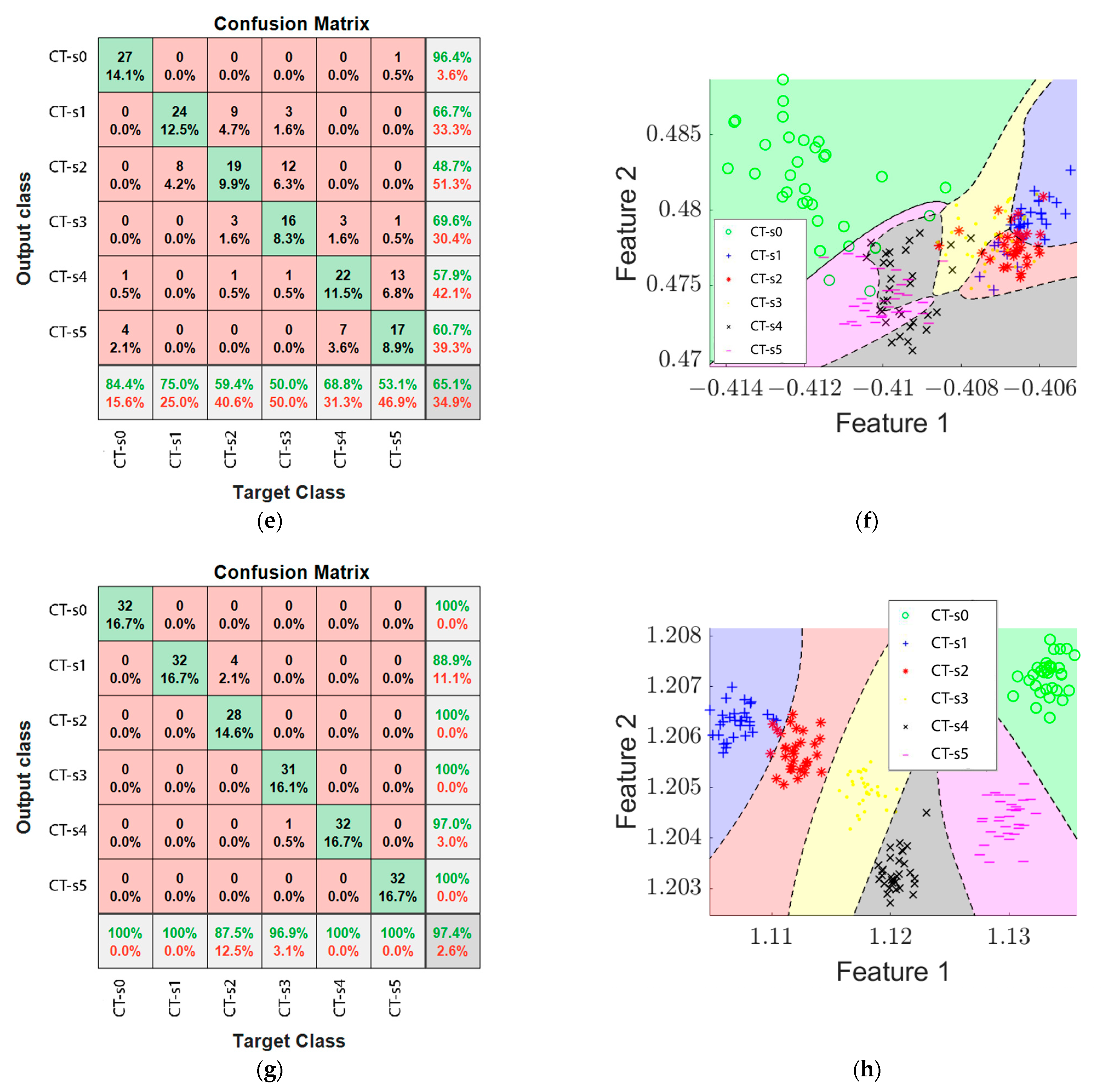
On the other hand, Table 7 presents the analysis results of the feed rate tests. With these results, it is possible to observe that for the tool feed rate experiments, the lowest contribution to wear identification accuracy is from the magnetic stray flux signal, adding 3.32% to the surface images accuracy and 4.48% when merged with the current data, but reducing the effectiveness by 2.8% when fused with image and current data. On the contrary, the image analysis presented the highest accuracy for identification of tool wear for the feed rate variations in contrast to the other signals.
When comparing the results obtained for both case studies, it is possible to observe an overall reduction in efficiency for the classification in the tool feed rate tests, this could be caused due to the effect of the variation in this parameter in the cutting process, as it changes the speed at which the tool travels through the workpiece and causes changes in the spacing of the cuts and the appearance of the grooves in addition to the effect of tool wear. In contrast, in the cutting speed case, the feed rate is constant and the changes in the grooves are caused only by tool wear.
Table 8 presents a brief comparison of the results of the proposed methodology with some previously reported in the literature, where some of the sensors are invasive. The main differences between our work and most of the reported works are the non-invasive nature of the sensors used, the possibility to choose the signal to analyze during the machining process or after it is finished and the quality of the pieces that are evaluated. In addition, the number of variations for each of the machining parameters was individually modified to evaluate the effect they have on the detection of wear of cutting tools with the objective of generating a system that can correctly identify wear regardless of the changes in the parameters.
These results show the potential of this methodology, as the effectiveness of the identification of tool wear through the fusion of different signals was increased. In addition, it is a non-invasive methodology for the machining process as it uses signals captured during the machining operations without the need to interrupt them and images of the surface finish of the parts are captured once operations are finished.

6. Conclusions

This paper proposes a non-invasive methodology based on the fusion of signals from the spindle motor of a CNC lathe and the analysis of the surface finish of the machined parts for the generation of a system. This allows the identification of wear with the individual variation of two important machining parameters with the possibility to analyze a single source or a combination of them according to the user’s needs and preferences without interrupting the process.
For the variation in cutting speed, the proposed methodology was able to identify the six levels of tool wear with an accuracy of 77.50% after analysis of the workpiece surface, 89.78% after analysis of stray flux signals and 73.02% after AC current signal analysis, with a peak efficiency of 95.02% after analysis of the fusion of surface images and stray flux signals.
For the variation in tool feed rate, the proposed system achieved a 76.34% effectiveness when using image analysis, 63.12% when analyzing stray flux signals and 73.0% when analyzing AC current signals, achieving a peak accuracy of 82.84% when analyzing both surface images and current signals.
For each of the case studies, it was possible to observe a different contribution of the signals for wear classification, achieving better results by including the magnetic stray flux within the information to be analyzed for the case of cutting speed tests and a better classification by including image analysis for the tool feed rate tests.
Additionally, it was noticed that the variation in the tool feed rate affects the formation of grooves when removing material from the workpiece, on top of the effect of tool wear, which makes it more difficult for the proposed system to correctly identify and classify tool wear in the tools used.
In future work, other non-invasive sensors, such as sound or AE, could be used to increase the number of information sources for a more robust analysis. Information processing could also be improved by applying other indicators and extracting more information or features from the surface images or by applying different classification techniques backed by the literature in order to improve the effects of using cutting parameters in the identification of tool wear. Additionally, with the knowledge of the effect of the tool feed rate on groove formation, a new approach could be developed to improve the wear identification while varying this parameter.

Author Contributions

G.D.-S. contributed to the writing of most of the paper, developed the methodology and the experimental setup and generated and analyzed the data; R.A.O.-R. conceived and developed the idea of this research, developed the methodology presented and contributed to the writing of most of the paper; I.Z.-R. developed the experimental setup, generated and analyzed the data and contributed to the writing of a section of the paper; I.A.C.-A. contributed to the development of the methodology, contributed to the writing of a section of the paper and analyzed the data; M.T.-H. developed the experimental setup, generated the data and contributed to the development of the methodology and data analysis; J.A.A.-D. conceived and developed the idea of this research, performed data analysis and contributed to the writing of a section of the paper. All authors have read and agreed to the published version of the manuscript.

Funding

This research was funded by the Spanish ‘Ministerio de Ciencia e Innovación’, Agencia Estatal de Investigación and FEDER program in the framework of the ‘Proyectos de Generación de Conocimiento 2021’ of the “Programa Estatal para Impulsar la Investigación Científico-Técnica y su Transferencia”, belonging to the “Plan Estatal de Investigación Científica, Técnica y de Innovación 2021–2023” (ref: PID2021-122343OB-I00).

Data Availability Statement

No new data were created or analyzed in this study. Data sharing is not applicable to this article.

Acknowledgments

The authors would like to thank Consejo Nacional de Ciencia y Tecnologia, CONACyT Scholarship with key code 2023-000002-01NACF-02215.

Conflicts of Interest

The authors declare no conflict of interest.

References

  1. Haraguchi, N.; Cheng, C.F.C.; Smeets, E. The importance of manufacturing in economic development: Has this changed? World Dev. 2017, 93, 293–315. [Google Scholar] [CrossRef]
  2. Ghosh, S.; Naskar, S.K.; Mandal, N.K. Estimation of residual life of a cutting tool used in a machining process. In MATEC Web of Conferences; EDP Sciences: Les Ulis, France, 2018; Volume 192, p. 01017. [Google Scholar]
  3. Zou, Z.; Lin, Y.; Lin, D.; Gu, F.; Ball, A.D. Online Tool Condition Monitoring of CNC Turnings based on Motor Current Signature Analysis. In Proceedings of the 2021 26th International Conference on Automation and Computing (ICAC), Portsmouth, UK, 2–4 September 2021; IEEE: Piscataway, NJ, USA, 2021; pp. 1–6. [Google Scholar]
  4. Marani, M.; Zeinali, M.; Songmene, V.; Mechefske, C.K. Tool wear prediction in high-speed turning of a steel alloy using long short-term memory modelling. Measurement 2021, 177, 109329. [Google Scholar] [CrossRef]
  5. Tabaszewski, M.; Twardowski, P.; Wiciak-Pikuła, M.; Znojkiewicz, N.; Felusiak-Czyryca, A.; Czyżycki, J. Machine Learning Approaches for Monitoring of Tool Wear during Grey Cast-Iron Turning. Materials 2022, 15, 4359. [Google Scholar] [CrossRef] [PubMed]
  6. Patange, A.D.; Jegadeeshwaran, R.; Bajaj, N.S.; Khairnar, A.N.; Gavade, N.A. Application of machine learning for tool condition monitoring in turning. Sound Vib. 2022, 56, 127–145. [Google Scholar] [CrossRef]
  7. Bombiński, S.; Kossakowska, J.; Jemielniak, K. Detection of accelerated tool wear in turning. Mech. Syst. Signal Process. 2022, 162, 108021. [Google Scholar] [CrossRef]
  8. Salodkar, S.M. On Line Robust Tool Wear Estimation during Turning of En31alloy Steel Using AE Sensor and Artificial Neural Network. J. Algebraic Stat. 2022, 13, 1607–1618. [Google Scholar]
  9. Casal-Guisande, M.; Comesaña-Campos, A.; Pereira, A.; Bouza-Rodríguez, J.B.; Cerqueiro-Pequeño, J. A decision-making methodology based on expert systems applied to machining tools condition monitoring. Mathematics 2022, 10, 520. [Google Scholar] [CrossRef]
  10. Rakkiyannan, J.; Jakkamputi, L.; Thangamuthu, M.; Patange, A.D.; Gnanasekaran, S. Development of Online Tool Wear-Out Detection System Using Silver–Polyester Thick Film Sensor for Low-Duty Cycle Machining Operations. Sensors 2022, 22, 8200. [Google Scholar] [CrossRef]
  11. Brili, N.; Ficko, M.; Klančnik, S. Tool condition monitoring of the cutting capability of a turning tool based on thermography. Sensors 2021, 21, 6687. [Google Scholar] [CrossRef]
  12. Sawangsri, W.; Wattanasinbumrung, P. A model approach for in-process tool condition monitoring in CNC turning using machine vision. Int. J. Interact. Des. Manuf. 2022, 16, 1439–1456. [Google Scholar] [CrossRef]
  13. Bagga, P.J.; Makhesana, M.A.; Darji, P.P.; Patel, K.M.; Pimenov, D.Y.; Giasin, K.; Khanna, N. Tool life prognostics in CNC turning of AISI 4140 steel using neural network based on computer vision. Int. J. Adv. Manuf. Technol. 2022, 123, 3553–3570. [Google Scholar] [CrossRef]
  14. Shen, L.C.; Kiow, L.W. Prediction Of Surface Roughness and Tool Wear from The Machined Surface by Machine Vision Approach. Res. Prog. Mech. Manuf. Eng. 2022, 3, 708–714. [Google Scholar]
  15. Kou, R.; Lian, S.W.; Xie, N.; Lu, B.E.; Liu, X.M. Image-based tool condition monitoring based on convolution neural network in turning process. Int. J. Adv. Manuf. Technol. 2022, 119, 3279–3291. [Google Scholar] [CrossRef]
  16. Bagga, P.J.; Makhesana, M.A.; Patel, H.D.; Patel, K.M. Indirect method of tool wear measurement and prediction using ANN network in machining process. Mater. Today Proc. 2021, 44, 1549–1554. [Google Scholar] [CrossRef]
  17. Kuntoğlu, M.; Sağlam, H. Investigation of signal behaviors for sensor fusion with tool condition monitoring system in turning. Measurement 2021, 173, 108582. [Google Scholar] [CrossRef]
  18. Hoang, D.T.; Van Thien, N.; Pham, T.T.T.; Nguyen, T.D. Combined analysis of acoustic emission and vibration signals in monitoring tool wear, surface quality and chip formation when turning SCM440 steel using MQL. EUREKA Phys. Eng. 2023, 86–101. [Google Scholar] [CrossRef]
  19. Jaen-Cuellar, A.Y.; Osornio-Ríos, R.A.; Trejo-Hernández, M.; Zamudio-Ramírez, I.; Díaz-Saldaña, G.; Pacheco-Guerrero, J.P.; Antonino-Daviu, J.A. System for tool-wear condition monitoring in cnc machines under variations of cutting parameter based on fusion stray flux-current processing. Sensors 2021, 21, 8431. [Google Scholar] [CrossRef]
  20. Diaz-Saldaña, G.; Osornio-Rios, R.A.; Cruz-Albarran, I.A.; Trejo-Hernandez, M.; Antonino-Daviu, J.A. CNC lathe tool wear analysis using image processing and stray flux. In Proceedings of the IECON 2022–48th Annual Conference of the IEEE Industrial Electronics Society, Brussels, Belgium, 17–20 October 2022; IEEE: Piscataway, NJ, USA, 2022; pp. 1–6. [Google Scholar]
  21. Kuntoğlu, M.; Aslan, A.; Pimenov, D.Y.; Usca, Ü.A.; Salur, E.; Gupta, M.K.; Sharma, S. A review of indirect tool condition monitoring systems and decision-making methods in turning: Critical analysis and trends. Sensors 2020, 21, 108. [Google Scholar] [CrossRef]
  22. Mohamed, A.; Hassan, M.; M’Saoubi, R.; Attia, H. Tool condition monitoring for high-performance machining systems—A review. Sensors 2022, 22, 2206. [Google Scholar] [CrossRef]
  23. Colantonio, L.; Equeter, L.; Dehombreux, P.; Ducobu, F. A systematic literature review of cutting tool wear monitoring in turning by using artificial intelligence techniques. Machines 2021, 9, 351. [Google Scholar] [CrossRef]
  24. Zhou, Y.; Liu, C.; Yu, X.; Liu, B.; Quan, Y. Tool wear mechanism, monitoring and remaining useful life (RUL) technology based on big data: A review. SN Appl. Sci. 2022, 4, 232. [Google Scholar] [CrossRef]
  25. Stojanović, B.; Gajević, S.; Kostić, N.; Miladinović, S.; Vencl, A. Optimization of parameters that affect wear of A356/Al2O3 nanocomposites using RSM, ANN, GA and PSO methods. Ind. Lubr. Tribol. 2022, 74, 350–359. [Google Scholar] [CrossRef]
  26. Yankov, E.; Minev, R.; Tonchev, N.; Lazov, L. Determination of the optimal mode of laser surface marking of aluminium composite panels with CO2 laser. Tribol. Mater. 2022, 1, 114–119. [Google Scholar] [CrossRef]
  27. Kalpakjian, S.; Schmid, S.R. Manufactura, Ingeniería y Tecnología; Pearson Educación: London, UK, 2008. [Google Scholar]
  28. Liu, H. Rail transit collaborative robot systems. In Robot Systems for Rail Transit Applications; Elsevier: Amsterdam, The Netherlands, 2020; pp. 89–141. [Google Scholar] [CrossRef]
  29. Distante, A.; Distante, C. Handbook of Image Processing and Computer Vision: Volume 1: From Energy to Image; Springer: Cham, Switzerland, 2020. [Google Scholar] [CrossRef]
  30. Bradley, D.; Roth, G. Adaptive thresholding using the integral image. J. Graph. Tools 2007, 12, 13–21. [Google Scholar] [CrossRef]
  31. Capolino, G.A.; Romary, R.; Hénao, H.; Pusca, R. State of the art on stray flux analysis in faulted electrical machines. In Proceedings of the 2019 IEEE Workshop on Electrical Machines Design, Control and Diagnosis (WEMDCD), Athens, Greece, 22–23 April 2019; IEEE: Piscataway, NJ, USA, 2019; Volume 1, pp. 181–187. [Google Scholar]
  32. Romary, R.; Pusca, R.; Lecointe, J.P.; Brudny, J.F. Electrical machines fault diagnosis by stray flux analysis. In Proceedings of the 2013 IEEE Workshop on Electrical Machines Design, Control and Diagnosis (WEMDCD), Paris, France, 11–12 March 2013; IEEE: Piscataway, NJ, USA, 2013; pp. 247–256. [Google Scholar]
  33. Zamudio-Ramirez, I.; Osornio-Rios, R.A.; Antonino-Daviu, J. Triaxial smart sensor based on the advanced analysis of stray flux and currents for the reliable fault detection in induction motors. In Proceedings of the 2020 IEEE Energy Conversion Congress and Exposition (ECCE), Detroit, MI, USA, 11–15 October 2020; IEEE: Piscataway, NJ, USA, 2020; pp. 4480–4484. [Google Scholar]
  34. Saucedo-Dorantes, J.J.; Delgado-Prieto, M.; Osornio-Rios, R.A.; Romero-Troncoso, R.D.J. Diagnosis methodology for identifying gearbox wear based on statistical time feature reduction. Proc. Inst. Mech. Eng. Part C J. Mech. Eng. Sci. 2018, 232, 2711–2722. [Google Scholar] [CrossRef] [Green Version]
  35. Deng, K. Fractal. In Encyclopedia of Database Systems, 2nd ed.; Liu, L., Özsu, T.M., Eds.; Springer: New York, NY, USA, 2018. [Google Scholar] [CrossRef]
  36. Amezquita-Sanchez, J.P.; Valtierra-Rodriguez, M.; Perez-Ramirez, C.A.; Camarena-Martinez, D.; Garcia-Perez, A.; Romero-Troncoso, R.J. Fractal dimension and fuzzy logic systems for broken rotor bar detection in induction motors at start-up and steady-state regimes. Meas. Sci. Technol. 2017, 28, 075001. [Google Scholar] [CrossRef]
  37. Higuchi, T. Approach to an irregular time series on the basis of the fractal theory. Phys. D Nonlinear Phenom. 1988, 31, 277–283. [Google Scholar] [CrossRef]
  38. Katz, M.J. Fractals and the analysis of waveforms. Comput. Biol. Med. 1988, 18, 145–156. [Google Scholar] [CrossRef]
  39. Antonino-Daviu, J.; Razik, H.; Quijano-Lopez, A.; Climente-Alarcon, V. Detection of rotor faults via transient analysis of the external magnetic field. In Proceedings of the IECON 2017-43rd Annual Conference of the IEEE Industrial Electronics Society, Beijing, China, 29 October–1 November 2017; IEEE: Piscataway, NJ, USA, 2017; pp. 3815–3821. [Google Scholar]
  40. Shannon, C.E. A Mathematical Theory of Communication. Bell Syst. Tech. J. 1948, 27, 379–423. [Google Scholar] [CrossRef] [Green Version]
  41. Rizal, A.; Hidayat, R.; Nugroho, H.A. Multilevel wavelet packet entropy: A new strategy for lung sound feature extraction based on wavelet entropy. In Proceedings of the 2017 International Conference on Robotics, Automation and Sciences (ICORAS), Melaka, Malaysia, 27–29 November 2017; IEEE: Piscataway, NJ, USA, 2017; pp. 1–5. [Google Scholar]
  42. Ding, C. Dimension Reduction Techniques for Clustering. In Encyclopedia of Database Systems, 2nd ed.; Liu, L., Özsu, T.M., Eds.; Springer: New York, NY, USA, 2018. [Google Scholar] [CrossRef] [Green Version]
  43. Yu, C.H.A. Data Mining and Exploration: From Traditional Statistics to Modern Data Science; CRC Press: Boca Raton, FL, USA, 2022. [Google Scholar]
  44. Tan, P.N. Neural Networks. In Encyclopedia of Database Systems, 2nd ed.; Liu, L., Özsu, T.M., Eds.; Springer: New York, NY, USA, 2018. [Google Scholar] [CrossRef]
  45. Han, J.; Kamber, M.; Pei, J. Data Mining Concepts and Techniques, 3rd ed.; Mechanical Industry Press: Beijing, China, 2012. [Google Scholar]
  46. Specification for Aluminum and Aluminum-Alloy Sheet and Plate (Metric) (Report); B07 Committee; ASTM International: West Conshohocken, PA, USA, 2014. [CrossRef]
  47. James, J.F. A Student’s Guide to Fourier Transforms: With Applications in Physics and Engineering, 3rd ed.; Cambridge University Press: Cambridge, UK, 2011. [Google Scholar]
  48. Polikar, R. The Wavelet Tutorial. 1996. Available online: https://users.rowan.edu/~polikar/WTtutorial.html (accessed on 10 March 2023).
  49. Zamudio-Ramirez, I.; Osornio-Rios, R.A.; Trejo-Hernandez, M.; Romero-Troncoso, R.D.J.; Antonino-Daviu, J.A. Smart-sensors to estimate insulation health in induction motors via analysis of stray flux. Energies 2019, 12, 1658. [Google Scholar] [CrossRef] [Green Version]
  50. Hsu, C.-C.; Lu, M.-C.; Wang, W.-Y.; Lu, Y.-Y. Distance Measurement Based on Pixel Variation of CCD Images. ISA Trans. 2009, 48, 389–395. [Google Scholar] [CrossRef] [PubMed]
  51. Dwivedi, R.; Gangwar, S.; Saha, S.; Jaiswal, V.K.; Mehrotra, R.; Jewariya, M.; Mona, G.; Sharma, R.; Sharma, P. Estimation of Error in Distance, Length, and Angular Measurements Using CCD Pixel Counting Technique. Mapan 2021, 36, 313–318. [Google Scholar] [CrossRef]
  52. Dutta, S.; Pal, S.K.; Mukhopadhyay, S.; Sen, R. Application of Digital Image Processing in Tool Condition Monitoring: A Review. CIRP J. Manuf. Sci. Technol. 2013, 6, 212–232. [Google Scholar] [CrossRef]
  53. Bagga, P.J.; Makhesana, M.A.; Patel, K.; Patel, K.M. Tool Wear Monitoring in Turning Using Image Processing Techniques. Mater. Today 2021, 44, 771–775. [Google Scholar] [CrossRef]
  54. Arévalo-Ruedas, J.H.; Espinel-Blanco, E.; Florez-Solano, E. Wear analysis in cutting tools by the technique of image processing with the application of two-dimensional matrices. J. Phys. Conf. Ser. 2021, 2139, 012018. [Google Scholar] [CrossRef]
Figure 1. Common placements for the use of coil sensors to capture magnetic stray flux signals in their radial and axial components: (a) view from the radial plane; (b) view from the axial plane.
Machines 11 00480 g001
Figure 2. Proprietary triaxial stay flux sensor used to capture the CNC lathe’s spindle motor signals, with the primary sensing elements indicated with a red ellipse.
Machines 11 00480 g002
Figure 3. Experimental setup: (a) CNC location of the DAS for the capturing of the current and stray flux signals, spindle motor showing details of the colocation of the stray flux sensors on the spindle motor and work area for the tests; (b) close-up of the DAS components: AC current clamp, ADC and microcontroller.
Machines 11 00480 g003
Figure 4. Aluminum bars used for the experiments: (a) bar machined for the cutting speed test using the tool with no wear; (b) piece machined for the cutting speed test with the tool with the largest wear; (c) part machined for the feed rate test with the tool with no wear; (d) workpiece machined for the feed rate test with the tool presenting the greatest wear.
Machines 11 00480 g004
Figure 5. Block diagram for the proposed methodology.
Machines 11 00480 g005
Figure 6. Stray flux and current signal feature extraction process.
Machines 11 00480 g006
Figure 7. Process followed for image analysis: (a) diagram showing the different steps of image processing to achieve the measurement of the grooves in the workpiece; (b) pseudocode indicating the steps followed by the automated image processing algorithm.
Machines 11 00480 g007aMachines 11 00480 g007b
Figure 8. Cutting tools used for the cutting speed experiments: (a) CT-s0; (b) CT-s1; (c) CT-s2; (d) CT-s3; (e) CT-s4; (f) CT-s5.
Machines 11 00480 g008
Figure 9. Cutting tools used for the tool feed rate experiments: (a) CT-f0; (b) CT-f1; (c) CT-f2; (d) CT-f3; (e) CT-f4; (f) CT-f5.
Machines 11 00480 g009
Figure 10. Current and stray flux signals measured during the 100 m/rev test with the CT-s5 tool: (a) original signals; (b) conditioned signals.
Machines 11 00480 g010
Figure 11. Micrographs taken of some of the machined specimens using the tool CT-s5: (a) for the test at 60 m/rev; (b) for the test at 80 m/rev; (c) for the test at 100 m/rev.
Machines 11 00480 g011
Figure 12. Confusion matrices and classification results obtained for the 100 m/rev tests: (a) confusion matrix for image analysis; (b) classification of tool wear for image analysis; (c) confusion matrix for stray flux analysis; (d) classification of tool wear for stray flux analysis; (e) confusion matrix for current analysis; (f) classification of tool wear for current analysis; (g) confusion matrix for image, current and stray flux fusion; (h) classification of tool wear for image, current and stray flux fusion.
Machines 11 00480 g012aMachines 11 00480 g012b
Figure 13. Current and stray flux signals measured during the 0.24 mm/rev test with the CT-f5 tool: (a) original signals; (b) conditioned signals.
Machines 11 00480 g013
Figure 14. Micrographs taken of some of the machined specimens from the tool feed rate tests using the tool CT-f5: (a) for the test at 0.08 mm/rev; (b) for the test at 0.16 mm/rev; (c) for the test at 0.24 mm/rev.
Machines 11 00480 g014
Figure 15. Confusion matrices and classification results obtained for the 0.24 mm/rev tests: (a) confusion matrix for image analysis; (b) classification of tool wear for image analysis; (c) confusion matrix for stray flux analysis; (d) classification of tool wear for stray flux analysis; (e) confusion matrix for current analysis; (f) classification of tool wear for current analysis; (g) confusion matrix for image, current and stray flux fusion; (h) classification of tool wear for image, current and stray flux fusion.
Machines 11 00480 g015aMachines 11 00480 g015bMachines 11 00480 g015c
Table 1. Set of statistical features used for the analysis of the signals.
Statistical FeaturesEquation
Mean x ¯ = 1 n i = 1 n x i (7)
Maximum value x ^ = max x (8)
Root Mean Square x R M S = 1 n i = 1 n x i 2 (9)
Square Root Mean x S R M = 1 n i = 1 n x i 2 (10)
Standard Deviation σ = 1 n i = 1 n x i x ¯ 2 (11)
Variance σ 2 = 1 n i = 1 n x i x ¯ 2 (12)
RMS Shape Factor S F R M S = x R M S 1 n i = 1 n x i (13)
SRM Shape Factor S F S R M = x S R M 1 n i = 1 n x i (14)
Crest Factor C F = x ^ x R M S (15)
Latitude Factor L F = x ^ x S R M (16)
Impulse Factor I F = x ^ 1 n i = 1 n x i (17)
Skewness S k = E x μ 3 σ 3 (18)
Kurtosis k = E x μ 4 σ 4 (19)
Fifth Moment 5 t h M = E x μ 5 σ 5 (20)
Sixth Moment 6 t h M = E x μ 6 σ 6 (21)
Table 2. 6061 Aluminum alloy composition by mass [46].
Constituent ElementAlMgSiFeCuCrZnTiMnOthers
% by weight95.85–98.56%0.80–1.20%0.40–0.80%0–0.70%0.15–0.40%0.04–0.35%0–0.25%0–0.15%0–0.15%0–0.15%
Table 3. Machining parameters used for the cutting speed variation tests.
No.d (mm)f (mm/rev)V (m/rev)N (rpm)vf (mm/min)
11.250.1660779.53124.72
21.250.1670909.45145.51
31.250.16801039.37166.30
41.250.16901169.29187.08
51.250.161001299.22207.87
Table 4. Machining parameters used for the tool feed rate variation tests.
No.d (mm)f (mm/rev)V (m/rev)N (rpm)vf (mm/min)
11.250.08100779.53103.938
21.250.12100909.45155.907
31.250.161001039.37207.875
41.250.201001169.29259.844
51.250.241001299.22311.813
Table 5. Comparison of groove measurements and errors using different contrast enhancements and thresholds for the cutting speed test at 70 m/rev using the tool with a wear area of 1.7016 mm2.
Contrast Enhancement—ThresholdNumber of Pixels Upper Groove (px)Measurement of Upper Groove in mm (% Error)Number of Pixels of the Lower Groove (px)Measurement of Lower Groove in mm (% Error)
Gamma transformation—adaptive threshold (proposed)15.220.1127 (1.44)7.110.0526 (1.54)
Gamma transformation—Otsu14.660.1085 (2.34)7.660.0567 (9.45)
Histogram equalization—Otsu15.110.1119 (0.72)7.220.0534 (3.08)
Histogram equalization—adaptive threshold15.440.1143 (2.8)6.880.0509 (1.73)
Table 6. Effectiveness results for the classification of tool wear with the use of the FFNN for the cutting speed tests.
V (m/rev)Surface ImagesAxial + Radial Stray FluxAC CurrentImages + Stray Flux FusionImages + AC Current FusionAC Current + Stray Flux FusionImages + AC Current + Stray Flux Fusion
6075.078.668.283.372.980.282.3
7084.991.182.399.093.292.2100.0
8063.095.378.199.082.896.494.8
9080.787.571.496.486.594.895.8
10083.996.465.197.487.097.997.4
Average77.5089.7873.0295.0284.4892.394.06
Table 7. Effectiveness results for the classification of tool wear with the use of the FFNN for the tool feed rate tests.
f (mm/rev)Surface ImagesAxial + Radial Stray FluxAC CurrentImages + Stray Flux FusionImages + AC Current FusionAC Current + Stray Flux FusionImages + AC Current + Stray Flux Fusion
0.0874.557.385.473.491.792.788.0
0.1288.567.272.485.493.872.982.8
0.1674.564.665.188.580.280.287.0
0.2070.863.076.066.174.070.866.1
0.2473.463.566.184.974.570.878.1
Average76.3463.1273.079.6682.8477.4880.4
Table 8. Comparison of the proposed methodology to systems reported in the literature.
SystemNumber of Wear Conditions EvaluatedSignals AnalyzedAchieved AccuracyMachining ParametersOnline/Offline
[6]6Vibrations92.6%Fixed value for cutting speed, tool feed rate and depth of cutOnline
[11]4Thermographs96%Fixed value for cutting speed, tool feed rate and depth of cutOnline
[15]6Vibration and current91%Nine experiments with three variations of cutting speed, tool feed rate and depth of cutOnline
[19]3Stray flux and AC current94.4%Cutting speed (five variations)Online
394.4%Tool feed rate (five variations)
Proposed Method6Surface images, AC current and stray flux95.02%Cutting speed (five variations)Online/Offline
682.84%Tool feed rate (five variations)
Disclaimer/Publisher’s Note: The statements, opinions and data contained in all publications are solely those of the individual author(s) and contributor(s) and not of MDPI and/or the editor(s). MDPI and/or the editor(s) disclaim responsibility for any injury to people or property resulting from any ideas, methods, instructions or products referred to in the content.

