Article

Reinforcement Learning-Based Dynamic Zone Placement Variable Speed Limit Control for Mixed Traffic Flows Using Speed Transition Matrices for State Estimation

by
Filip Vrbanić
1,*,†,
Leo Tišljarić
1,2,†,
Željko Majstorović
1 and
Edouard Ivanjko
1
1
Faculty of Transport and Traffic Sciences, University of Zagreb, Vukelićeva Street, 4, HR-10000 Zagreb, Croatia
2
INTIS d.o.o., Bani 73a, Buzin, HR-10010 Zagreb, Croatia
*
Author to whom correspondence should be addressed.
These authors contributed equally to this work.
Machines 2023, 11(4), 479; https://doi.org/10.3390/machines11040479
Submission received: 27 February 2023 / Revised: 11 April 2023 / Accepted: 12 April 2023 / Published: 14 April 2023

Abstract

:
Current transport infrastructure and traffic management systems are overburdened due to the increasing demand for road capacity, which often leads to congestion. Building more infrastructure is not always a practical strategy to increase road capacity. Therefore, services from Intelligent Transportation Systems (ITSs) are commonly applied to increase the level of service. The growth of connected and autonomous vehicles (CAVs) brings new opportunities to the traffic management system. One of those approaches is Variable Speed Limit (VSL) control, and in this paper a VSL based on Q-Learning (QL) using CAVs as mobile sensors and actuators in combination with Speed Transition Matrices (STMs) for state estimation is developed and examined. The proposed Dynamic STM-QL-VSL (STM-QL-DVSL) algorithm was evaluated in seven traffic scenarios with CAV penetration rates ranging from 10 % to 100 % . The proposed STM-QL-DVSL algorithm utilizes two sets of actions that include dynamic speed limit zone positions and computed speed limits. The proposed algorithm was compared to no control, rule-based VSL, and two STM-QL-VSL configurations with fixed VSL zones. The developed STM-QL-DVSL outperformed all other control strategies and improved measured macroscopic traffic parameters like Total Time Spent ( T T S ) and Mean Travel Time ( M T T ) by learning the control policy for each simulated scenario.

1. Introduction

Due to population growth, the influence of the automotive industry, and car sales, the urban road network has been under the influence of increasing traffic demand in recent years. Congestion is the consequence of this increased demand, particularly during peak hours. Urban motorways, which serve as quick links between large urban areas in large cities or as city bypasses, are also affected by this increasing traffic demand. This occurs as a result of urban motorways’ high vehicle volume, originating from many simultaneous incoming traffic flows from on-ramps and the mainstream motorway flow. When these simultaneous traffic flows merge into the mainstream flow, the mainstream flow is disrupted, lowering the operational capacity, creating congestion, and diminishing the motorway’s safety. Building more lanes would seem to be the best way to boost operational capacity and reduce congestion. However, due to the cost and lack of space in cities, this solution is not always practical.
Utilizing traffic control services originating from Intelligent Transportation System (ITS) domain is another strategy. The operational capacity of an urban motorway can be improved by implementing suitable traffic control measures such as Variable Speed Limit (VSL) and ramp metering. The first measure is the focus of this paper. In a standard approach, it sets the best-computed speed limits on an urban motorway by using Variable Message Signs (VMS) that take into account the status of traffic flows and/or current meteorological conditions. VSL attempts to reduce the speed differences between the merging flow and the mainstream flow. In this way, congestion and the creation of shockwaves can be effectively limited or even eliminated [1].
Many techniques can be used to implement VSL. However, recently machine learning and Reinforcement Learning (RL) techniques have received a lot of attention [2]. As an illustration, an RL approach was used to optimize the control policy for the application of VSL [3]. The fundamental idea behind RL is to carry out the best-computed action in an acquired or predicted environment state based on the values of the state–action pairs that are continuously updated and learned. To evaluate the efficacy of the proposed techniques, Measures of Effectiveness (MoEs) such as Total Travel Time ( T T T ), Total Time Spent ( T T S ), Mean Travel Time ( M T T ), and total delay time are frequently measured. For example, in our previous paper [4], we used multi-agent-based distributed W-learning where each agent uses RL to learn local policies and remote policies to understand how actions affect their immediate neighbors while enforcing computed speed limits.
The development of Autonomous Vehicles (AVs) and Connected Autonomous Vehicles (CAVs) opens up new opportunities for traffic flow management. A new type of traffic flow known as a “mixed traffic flow” that involves Human-Driven Vehicles (HDVs), AVs, and CAVs with varied penetration rates is created as a result of such vehicles’ involvement in the existing traffic flows. CAVs have the capacity to transmit and receive data about traffic state. They are also described as having improved driving characteristics and great adherence to traffic laws [5]. In the previous paper [6], an overview of RL algorithms that were applied to optimize the VSL control algorithm in such mixed traffic flow conditions was given.
The proposed VSL for application on urban motorways was recently developed and uses CAVs acting as actuators for the VSL algorithm [5]. The VSL control policies that decreased T T T , M T T , and density in a bottleneck area and increased speed in a bottleneck area were optimized using the Q-Learning (QL) method. The proposed method for assessing traffic density and estimating the condition of urban motorways utilized induction loops. However, due to the fixed location of these detectors, traffic parameters were measured in a limited area, resulting in inefficiencies in VSL implementation. In our previous paper [7], a QL-VSL algorithm was developed to mitigate the negative environmental effects of traffic, with two alternative reward functions: proportional T T S and total energy consumption. Both configurations of QL-VSL demonstrated improvements in macroscopic traffic and ecological parameters compared to baseline scenarios, utilizing the same state estimate technique as was used in a previous paper [5]. The Speed Transition Matrix (STM) approach was applied for state representation in an STM-QL-VSL algorithm, and two speed limit zone configurations were analyzed and found to outperform both no-control scenarios and rule-based VSL [8]. In another paper [9], Full Cellular Activity (FCA) data were used to create an estimation model for detecting large-scale motorway traffic congestion. To improve the model’s accuracy, a wider range of FCA data was employed, resulting in successful identification of both small and large congestion. However, this method was limited to congestion detection and did not provide a means for alleviating congestion.
The communication capability of CAVs is used in this paper to implement an agent-based centralized traffic control approach. A QL-based VSL (QL-VSL) agent computes and posts the appropriate speed limit using its accumulated knowledge. Additionally, a mixed traffic flow containing only CAVs and HDVs in multiple varying traffic scenarios is examined as a replica of realistic future mixed traffic flows. Thus, it is assumed that the Road Side Units (RSUs) transmit speed limit information, which is received by CAVs only through an installed On-Board Unit (OBU). It is also assumed that the information transmission is error- and delay-free. Every CAV’s speed and position is recorded and used to provide a new approach for motorway traffic state estimation. It is based on STMs that measure the current speed of CAVs transitioning between two consecutive motorway segments [10]. In such a configuration, the CAVs are used as mobile sensors and actuators. The utilization of CAVs as mobile sensors eliminates the requirement for conventional traffic detectors, and their application as actuators eliminates the requirement for conventional VMS. By using CAVs as mobile sensors, it becomes possible to identify bottlenecks with greater accuracy on a longer motorway segment and to focus on the length and position of the bottleneck, resulting in improved bottleneck identification. Section 3.2 provides a comprehensive description of the proposed motorway traffic state estimation approach.
Therefore, this paper describes the developed Dynamic STM-QL-VSL (STM-QL-DVSL) that utilizes two sets of actions that include dynamic speed limit zone positions and computed speed limits to mitigate and reduce the negative effects of congestion. The proposed STM-QL-DVSL algorithm is compared to the no-control scenario and developed Rule-Based VSL (RB-VSL) algorithm, developed based on density and speed thresholds from the Highway Capacity Manual (HCM) levels of service [11]. The main contributions of this paper are the following:
  • Proposal of an approach that utilizes the QL algorithm for VSL that computes speed limits and speed limit zone positions that are imposed on CAVs;
  • Usage of STMs for environment state space approximation from the data collected from CAVs as an input to the QL algorithm that computes speed limits and speed limit zone positions;
  • Analysis of scenarios with different penetration rates of CAVs on the simulated urban motorway by using the proposed STM-QL-DVSL approach.
This paper is structured as follows. An overview of prior studies on VSL application on urban motorways is provided in Section 2. The proposed methodology is described in Section 3. An overview of the simulation model is given in Section 4 and the results including analysis and discussion of our simulations are presented in Section 5. The paper’s conclusion and any potential follow-up research are presented in the last section of this paper.

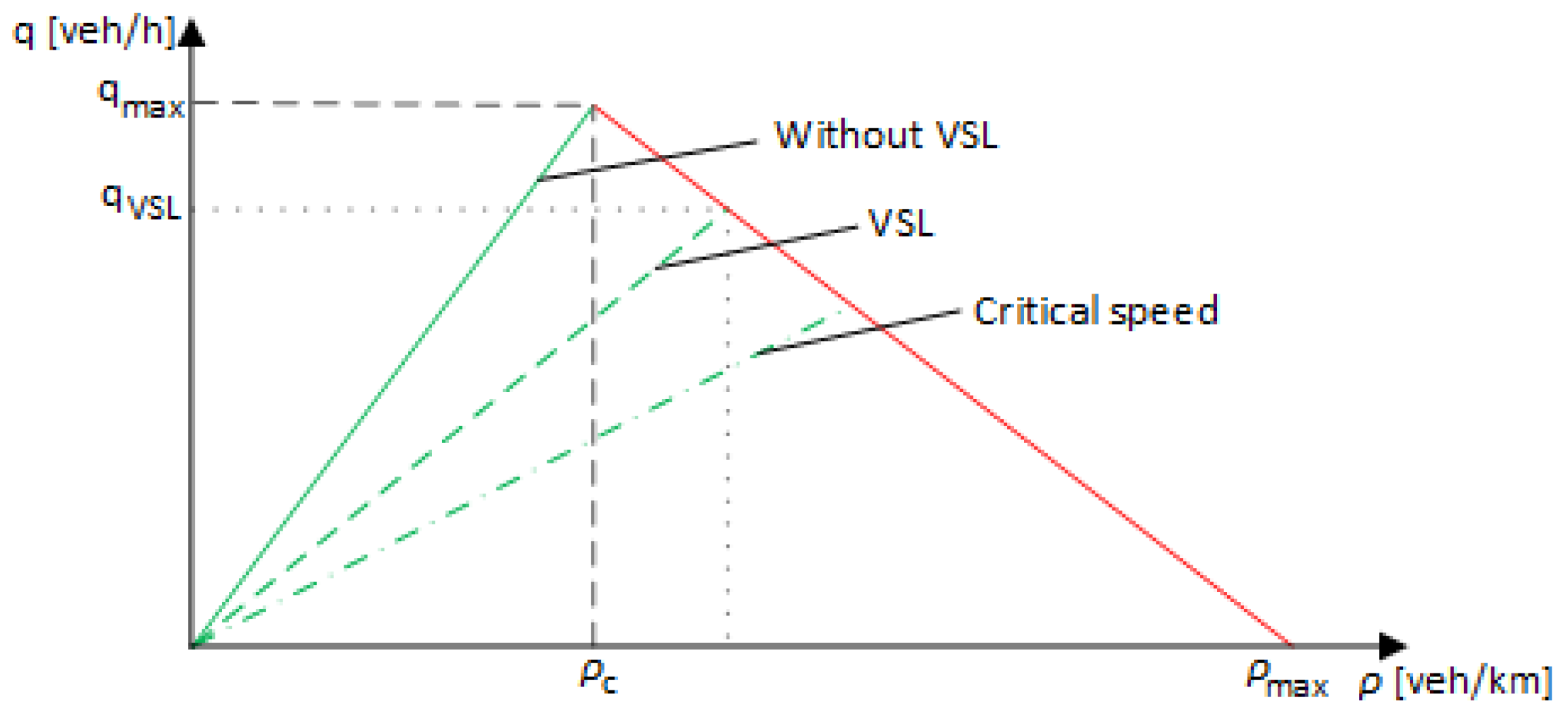
2. Variable Speed Limit

The VSL control approach aims to adjust the operational capacity of the bottleneck by setting suitable speed limits to regulate the incoming flow of vehicles moving toward the congested area [12]. In this way, further capacity drops can be prevented and the occurring congestion can be relieved more quickly. This, in turn, helps to maintain the traffic flow moving in the congested area near the maximal capacity value. To increase road throughput and safety, VSL is utilized to control vehicle speeds. The controlled road segment’s traffic flow is indirectly impacted by changing the speed limit on a VMS, and the speed of incoming vehicles into congested motorway sections is reduced [12]. As a result, the bottleneck area’s maximum capacity is not exceeded and the congestion is cleared more quickly or even avoided. This keeps the motorway’s capacity from dropping significantly. Speed homogenization that is achieved by using VSL also lowers the probability of accidents [13].
The basic fundamental diagram shown in Figure 1 depicts the relationship between traffic density ρ (shown on the x-axis) and flow q (shown on the y-axis) and is frequently used in the creation of VSL controllers. It is implied that lowering the speed limit increases the outflow of vehicles in the controlled area section by the authors’ quantitative explanation of the effect of VSL on the fundamental diagram in the previous paper [14]. According to the previous paper [15], a stable traffic flow has a reduced density without many disruptions between vehicles. When the traffic density reaches a value above the critical point, the traffic flow becomes unstable, amplifying the negative effects of interactions between vehicles.
The authors of the previous paper [16] examined the influence of various CAV penetration rates on the acceleration rate and speed disparities. The results showed that there were less noticeable disparities with the increase in CAV penetration rate from 0 to 100 % . The lane capacity was also impacted by the penetration of AVs and CAVs. Experimenting with various CAV penetration rates ranging from 0 to 100 % , it was observed that the lane capacity increased by 188.2 % , whilst the capacity increased nearly linearly [17]. Particularly, in a scenario with a penetration rate of 70 % of CAVs, the critical density increased by about 37 % , while the operational capacity increased by 42 % [18].

3. Variable Speed Limit Based on Q-Learning and Speed Transition Matrices

3.1. Q-Learning and Variable Speed Limit

The main idea behind the QL algorithm is to update Q-values stored in the Q-matrix, which represent state–action pairs when the environment conditions reach a certain state. To learn, the QL algorithm uses a feedback loop mechanism based on computing a given reward function that measures the effectiveness of the applied action a in an environment state s. The QL introduces some stochasticity into its behavior since if it were to run infinitely, it would globally choose the best possible action with the highest Q-value. The result of the QL execution generates the maximal possible Q-value for each state–action pair. Therefore, each state has the largest Q-value for the best possible action in that particular environment state. The Q-value is updated on every agent’s event of selecting the action in the environment state, according to [19]:
Q * ( s t , a t ) : = ( 1 α ) Q ( s t , a t ) + α ( r t + γ max a A Q ( s t + 1 , a ) ) ,
where the Q-value is represented as Q ( s t , a t ) computed for the state–action pair ( s t , a t ) at time step t. Then, the discount factor γ represents the importance of future rewards in the next state. The performed action a t is evaluated by reward r t + 1 in state s t . Furthermore, the next environment state is represented with s t + 1 , and α is the learning rate for determining the speed with which QL acquires new knowledge and updates Q-values.
The actual challenge solved by QL is to apply the best possible value of the speed limit using the VSL traffic control approach to make the traffic flow more harmonized and to relieve the congestion. The decision-making process can be described as a Markovian Decision Process of the agent’s decision to compute the speed limits as expressed in previous papers [2,5,20,21,22]. At each control timestamp t, actions are executed that trigger the feedback to the agent based on the environment state change via an appropriately defined reward function. The agent chooses an action a t , the appropriate speed limit value from a discrete set of actions A = { 60 , 70 , 80 , 90 , 100 , 110 , 130 } km/h, at an environment state s t . Setting the restriction of changing the speed in consecutive timestamps to a maximal range of ±30 km/h ensures compliance with the legislation and smooths the speed limit changes, with the aim of not causing sudden braking or acceleration. The learning rate α was updated according to [7,8]:
α ( s , a ) = 1 1 + n v ( s , a ) 0.8 + c ,
where the number of visits of each state–action pair is represented with n v ( s , a ) . Ensuring continuous learning, even after many traffic simulations, is enabled with parameter c as a constant value of 0.05.
For incorporating two look-ahead distant states, the standard QL algorithm (1) needed to be altered as described in previous papers [5,7]. Besides distant states, mapping of the speed limit and speed limit zone position was incorporated and expressed as
Q * ( s t , [ a , z ] t ) : = ( 1 α ) Q ( s t , [ a , z ] t ) + α ( s t , [ a , z ] t ) ( r t + λ r t + 1 + λ 2 max [ a , z ] A Q ( s t + 2 , [ a , z ] t + 2 ) ) ,
where z represents the selection of the speed limit zone position, and λ places emphasis on discrepancies based on a more distant look ahead and replaces the parameter γ of the original QL algorithm. In this QL algorithm variation, the agent also chooses the speed limit zone position z where the speed limit needs to be applied upstream to the merging area on the motorway. This is an improvement to classic approaches where only speed limit values are computed. The [ a , z ] matrix represents the set of all available actions that include the speed limit a from the set of available actions A, and the speed limit zone position z from a set of available speed limit zone positions Z = { 4.5 5.0 , 4.55 5.05 , 4.6 5.1 , 4.65 5.15 , 4.7 5.2 } km. Each available speed limit zone z has a fixed length of 500 m. In this instance of QL, the agent chooses the appropriate speed limit and speed limit zone position for a given state. The importance of future environment states for the learning agent was determined by a sensitivity analysis and the parameter λ was set to 0.9 [7]. The trade-off between exploration and exploitation was established using the ϵ - g r e e d y policy, where a random speed limit action a and a random speed limit zone position z are selected for a given state s from a set of available actions A and Z when the ϵ value is very high. The ϵ value was updated using a sigmoid function expressed as
ϵ = 0.95 1 + ( e ( n 50 ) ) 0.1 + 0.05 ,
where the current simulation iteration is represented with n. Thus, to determine the state–action pair Q value, the parameter ϵ is modeled to gain high exploration probability at the start of the learning process. To model this behavior, the ϵ in the first 30 simulations is set to ≥0.9 to ensure a high probability of selecting random actions. To ensure a slow decrease in the probability of random action selection, the ϵ value drops from 30th to 100th simulation to the constant value of 0.05 . The rewards for the QL algorithm were computed based on reducing the TTS at the upstream flow area, which was influenced by reducing the bottleneck probability of occurrence and length. This reward setup encourages the algorithm to minimize the TTS, which leads to relieving the effects of congestion and preventing bottleneck occurrences.

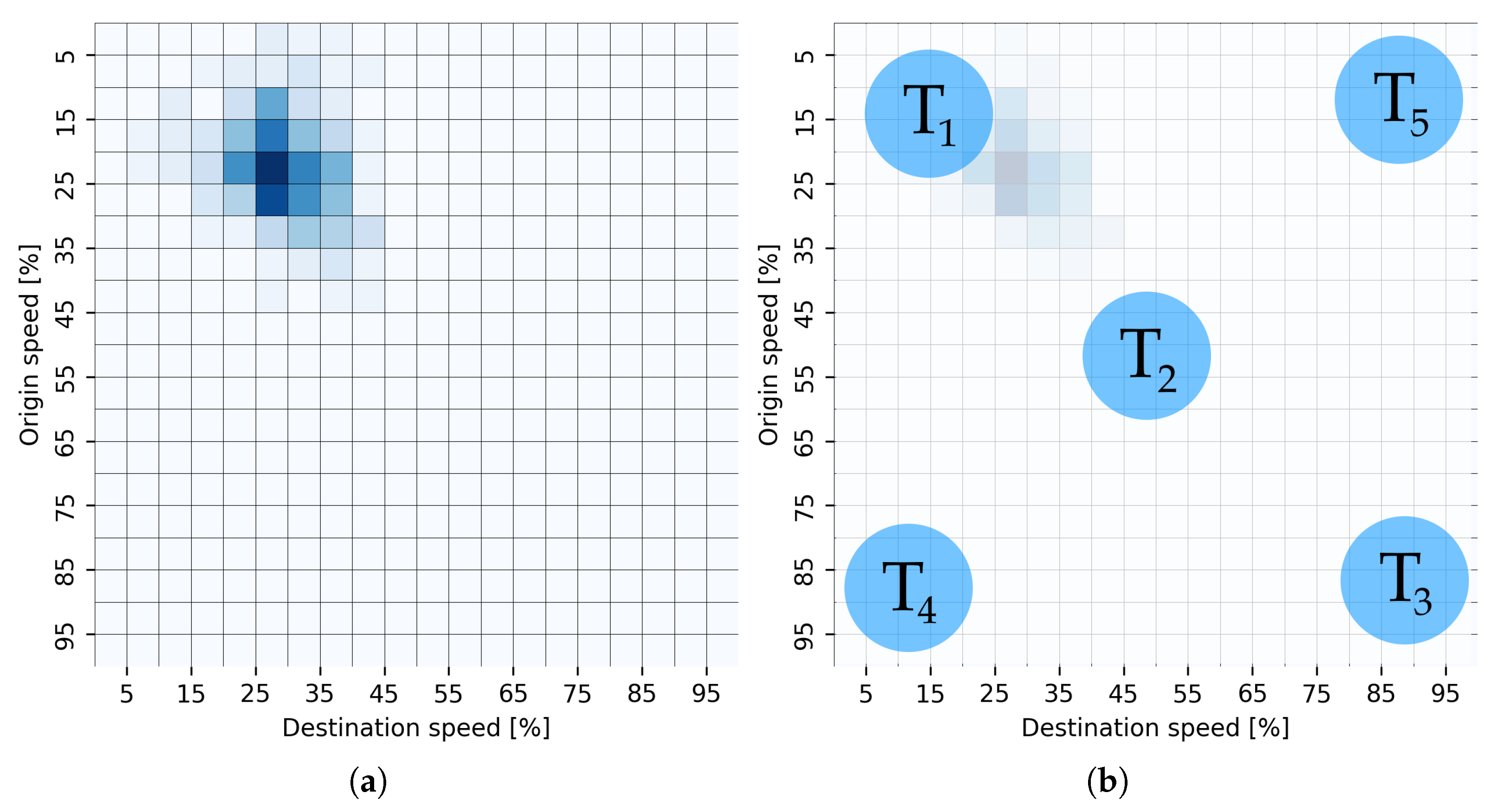
3.2. State Space Representation Using Speed Transition Matrices

The proposed approach is based on the use of the STM-based method for determining the traffic state [8], which is then used as the motorway state space representation. STM is a traffic data representation that has recently emerged [10,23] as a method that incorporates spatial and temporal motorway traffic data in the form of a matrix. The matrix represents the probability of vehicle speed change at the observed transition between two consecutive motorway segments e i and e j , where speeds are measured for every vehicle passing through this transition point inside a time interval Δ t . One transition is then defined within the examined time interval Δ t , where e i represents the origin road segment with its corresponding vehicle speeds v i , and e j represents the destination road segment with corresponding vehicle speeds v j . The STM can be then expressed as
X ( Δ t ) = p ( 11 ) p ( 1 n ) p ( m 1 ) p ( m n ) ,
where each cell p i j represents the probability of the speed change from v i to v j at the observed transition between road segments e i and e j within the time interval Δ t . The most important feature extracted from the STM is the underlying traffic pattern represented in a matrix form. An example of the so-created STMs can be observed in Figure 2a showing the extracted traffic pattern representing a congested traffic flow. On the other hand, Figure 2b represents other characteristic positions at which the estimated traffic pattern can be placed. At positions T 1 , T 2 , and T 3 , the STM pattern represents congested, unstable, and free traffic flow, respectively. On the other hand, positions T 4 and T 5 represent anomalous traffic behavior like sudden braking and intense accelerations. These examples lead to the conclusion that STM patterns can be effectively used for traffic state representation on motorways as proved in our prior paper [8].
In this context, the STM is used to represent traffic patterns from which the motorway bottleneck probability p b is estimated based on the traffic pattern position inside the STM. The p b is a continuous variable in the range [0, 1], where 0 represents free traffic flow, and 1 represents traffic congestion. As the method is spatially related to two consecutive road segments, its results can be used to estimate the bottleneck’s impact and length. The p b is then discretized, by applying the method from the previous paper [24], to values 0, representing transitions with low bottleneck probability, and 1, representing high bottleneck probability. The discretization allows a simplification of traffic state representation and provides an interpretable method for estimating the bottleneck length on a motorway by counting the transitions with high bottleneck probability values. The total state of the congested motorway segments is then computed according to the sum of the traffic states at the upstream flow of the merging area where traffic flows from mainstream and on-ramp intersect.

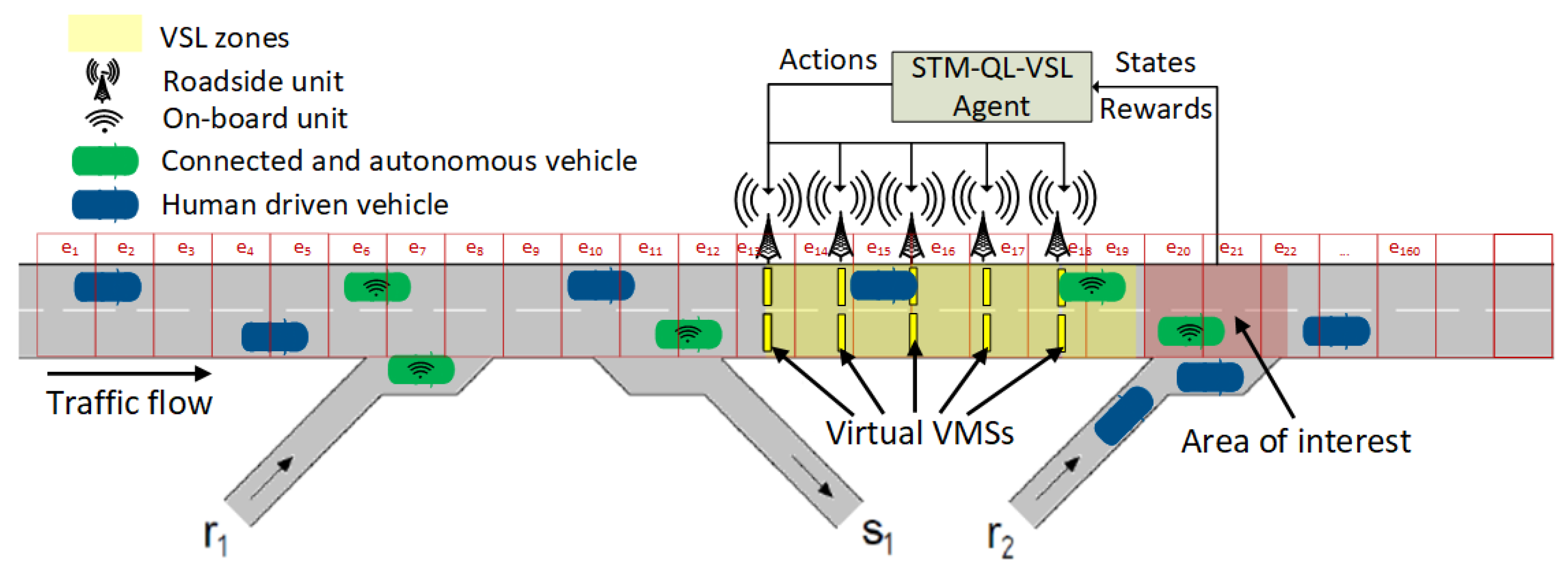
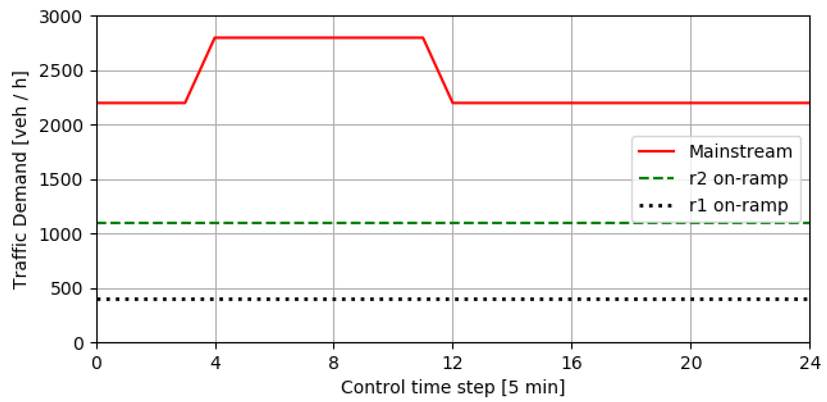
4. Simulation Framework

Using the model of a synthetic motorway from the previous paper [8] as shown in Figure 3, the effectiveness of the proposed STM-QL-DVSL algorithm was evaluated. It should be noted that the model presented in Figure 3 is not scaled to match the original model. Two on-ramps ( r 1 and r 2 ) and one off-ramp ( s 1 ) are present in the model (Figure 3). The length of the acceleration and deceleration lanes for on-ramps and off-ramp is set to 250 m, and the mainstream section does not contain any vertical slopes. The entire model is divided into 160 segmented edges e i creating consecutive segments, which are each 50 m long. The model has five possible dynamic VSL zone positions defined as Z. The simulations were carried out using the Simulation of Urban MObility (SUMO) microscopic traffic simulator [25]. The TraCI interface was used to externally implement the STM-QL-DVSL algorithm in a Python script, allowing for the collection of needed traffic measurements and direct control of the real-time simulation including posting computed speed limit values and dynamic speed limit zone positions. Every simulation scenario simulates 2 h of traffic with 24 control time steps, each lasting for 5 min. To mimic increasing demand during peak hours, the traffic demand was modeled as illustrated in Figure 4.
Traffic parameters were measured at 5 s intervals during each control time step (lasting 5 min), and mean values were obtained. Those obtained traffic parameters included density ( ρ ) measured in veh/km/ln, speed (v) measured in km/h, and M T T measured in s. In addition, T T S is expressed as veh·h, and it was measured cumulatively for the whole simulated motorway including on- and off-ramps, while ρ and v were measured for the specific area of interest (congestion zone) visible in Figure 3. On the other hand, M T T is measured only on the mainstream traffic direction, thus not including on- and off-ramps.
The SUMO simulator was also used to define vehicle class parameters and car-following models for both HDVs and CAVs, as already used in previous studies [5,8,26]. As mentioned before, CAVs are assumed to have smaller time headways, lower driver imperfection, and higher compliance with the imposed speed limits compared to the HDVs. The parameters for both vehicle classes are defined according to previously published studies since the real-world data for CAVs are not publicly available and hard to obtain without the ability to measure those parameters for such vehicles in a real-world experiment. Therefore, the driving imperfection parameter σ was set to 0.7 and 0 for HDVs and CAVs, respectively. Herein, value 0 represents perfect driving behavior, meaning that the lower σ value leads to more rigorous acceleration and deceleration actions. Speed limit deviation parameter S p e e d D e v represents the ratio of allowed deviation from the set speed limit and it was set to 0.2 and 0.05 for HDVs and CAVs, respectively. The lane speed limit multiplier parameter S p e e d F a c t o r was set to 1 for both HDVs and CAVs, as both lanes have the same speed limit. The vehicle’s desired (minimum) time headway parameter τ , which is based on the net time between leader back and follower front expressed in seconds, was set to 1.1 and 0.5 for HDVs and CAVs, respectively. Lower τ values were proven to increase the traffic flow [16,27]. Furthermore, the influence of CAV levels of automation based on σ and τ values have shown that as the CAV penetration rate of vehicles with lower σ and τ values increased, the road capacity of the overall network increased, and the ρ c value on a single road was higher [27]. The ρ c value was increased by almost 48 % from no CAVs to 100 % CAVs in mixed traffic flow according to the simulation example described in a previous paper [27]. The proposed STM-QL-DVSL method was evaluated in six simulation scenarios with different CAV penetration rates ranging from 10 % to 100 % .

5. Results and Discussion

Simulations for the no control scenario were conducted with a fixed speed limit of 130 km/h. STM-QL-DVSL policy for the latter was trained by running 2000 simulations for each mixed traffic flow scenario. The performance of the STM-QL-DVSL algorithm was compared to the performance of other control algorithms, including STM-QL-VSL 1 , STM-QL-VSL 2 [8], and RB-VSL, as well as to the no-control scenario. The RB-VSL algorithm was implemented based on previous works [5,7,8], following the HCM levels of service [11]. RB-VSL and STM-QL-DVSL differ primarily in their approach to VSL. RB-VSL employs traditional VMS to display speed limits to all vehicles, whereas STM-QL-DVSL uses CAVs that act as mobile sensors and actuators for VSL. The STM-QL-VSL 1 and STM-QL-VSL 2 algorithms, developed in a previous paper [8], use fixed speed limit zone positions. The STM-QL-VSL 1 algorithm enforces computed speed limits in one applicable speed limit zone closest to the area of interest. On the other hand, the STM-QL-VSL 2 algorithm enforces computed speed limits in two applicable speed limit zones directly adjacent to each other. The configuration of those two algorithms is described in more detail in the previous paper [8]. The main difference between STM-QL-DVSL and STM-QL-VSL 1 and STM-QL-VSL 2 is that the proposed algorithm in this paper dynamically selects the speed limit zone position instead of having the fixed position, as is the case with STM-QL-VSL 1 and STM-QL-VSL 2 algorithms. Thus, it presents a continuation of our previous research.
The results of all analyzed scenarios are presented in Table 1. The results are obtained from a selected representative simulation that represents an average simulation from the last 500 simulations for each mixed traffic flow scenario. Based on the findings, STM-QL-DVSL performed better than all other control strategies across all the simulated scenarios, particularly in terms of reducing T T S and M T T for the entire motorway section. On the other hand, the RB-VSL algorithm proved to be less effective than having no control strategy at all. The exception is scenario 2, where the predefined rules for changing the speed limit based on HCM level of service density thresholds were found to be effective. STM-QL-VSL 1 and STM-QL-VSL 2 showed more pronounced improvements at lower CAV penetration rates, which gradually reduced as the penetration rate increased. Moreover, the proposed STM-QL-DVSL algorithm was able to further improve MoEs at lower penetration rates, mainly due to the superior driving characteristics of CAVs as compared to HDVs and using traffic state measurements on the microscopic level (each CAV is a mobile sensor). However, as the number of CAVs in the mixed traffic flow increased, the positive effects of the STM-QL-DVSL algorithm were reduced.
The obtained results for scenarios 1 and 2, including the posted speed limits, ρ c , v c , and T T S , are shown in Figure 5. Again, the results are obtained from a selected representative simulation, which is an average simulation from the last 500 simulations after 2000 simulations were run for each mixed traffic flow scenario. Firstly, it can be observed that the proposed STM-QL-DVSL selected lower speed limits during increased traffic demand compared to other control algorithms. In scenario 1, STM-QL-DVSL showed a 3.0 % improvement in T T S compared to the no control scenario. In contrast, RB-VSL worsened the situation slightly by increasing T T S by 0.6 % . For scenario 1, STM-QL-VSL 1 and STM-QL-VSL 2 improved T T S by only 1.5 % and 0.1 % compared to no control, respectively. In scenario 2, the proposed STM-QL-DVSL outperformed all other strategies and improved T T S by 5.4 % . On the other hand, RB-VSL, STM-QL-VSL 1 , and STM-QL-VSL 2 reduced T T S by 2.3 % , 3.3 % , and 4.3 % , respectively. All RL-based VSL algorithms improved mean ρ , mean v, and M T T compared to both no control and RB-VSL control. Among them, STM-QL-DVSL performed the best. By using CAVs as actuators and state estimators for VSL on an urban motorway, the proposed STM-QL-DVSL method improved the overall MoEs. These observed improvements for scenario 2 indicate that with 30 % CAV penetration rate, the analyzed algorithms have sufficient input data used to estimate the traffic flow using STMs as observed in the previous paper [28]. A more accurate representation of the state of the traffic flow allows the agent to learn actions in the correctly represented discrete states, which improves the performance of all analyzed algorithms that use STMs as state representation. Those algorithms are, as mentioned, STM-QL-VSL 1 and STM-QL-VSL 2 and STM-QL-DVSL. Furthermore, the results indicate that as the CAV penetration rate increases from 30 % to 100 % , the influence of the increased number of CAVs on the analyzed algorithms’ performance is less pronounced at higher penetration rates. Thus, one can assume that the increase in the CAV penetration rate has the largest impact at small penetration rates. After enough input data from CAVs are available, the state estimation quality is sufficient for ensuring good operation of the developed VSL controller. In this paper, this happens with a penetration rate of 30 % , similar to the previously published analysis conducted in the previous paper [28]. Thus, the obtained improvements were more noticeable in scenarios 1 and 2, where the low CAV penetration rate provided sufficient data for state estimation and appropriate speed limit applications. Incorporating CAVs into mixed traffic flow had a positive impact on measures of T T S and M T T , as shown in Figure 6. These improvements are mainly credited to the improved driving performance of CAVs characterized by small vehicle headways and faster reaction time.
Significant improvements were observed in the mean ρ of the congested area, which can be attributed in part to the improved driving characteristics of CAVs. Additionally, the STM-QL-DVSL algorithm was found to reduce the speed of incoming vehicles in the area of interest, resulting in a reduction in the impact of merging maneuvers of on-ramp vehicles and a corresponding relaxation of shock-waves. This, in turn, allowed on-ramp vehicles to merge more quickly and safely into the mainstream flow, resulting in less pronounced interactions between vehicle flows and a reduction in the mean ρ in the area of interest. Notably, the proposed STM-QL-DVSL algorithm resulted in an 11.7 % improvement in mean ρ in scenario 3 compared to the no-control strategy. In a scenario with 100 % CAV penetration rate, the implemented VSL approaches had no effect on the traffic flow, indicating that the driving characteristics of CAVs alone were sufficient to maintain a free-flow state and obviate the need for additional traffic control algorithms for the simulated traffic demand case.
The selection of applicable speed limit zone position and the applied speed limits for scenario 1 and scenario 2 is shown in Figure 7. One observation is that the STM-QL-DVSL agent learned that the best applicable speed limit zone position is the one farthest from the congested area when the mainstream traffic flow is increased. In addition, the STM-QL-DVSL agent selected lower speed limits for scenario 1 compared to scenario 2. This indicates that slowing mainstream vehicles sooner and with lower speeds further improves MoEs by ensuring that vehicles are slowed earlier and their speeds are harmonized smoothly. Comparing the speed limit zone positions between these two scenarios, it is noticeable that as CAVs become more prevalent, the STM-QL-DVSL agent tends to clear congestion more quickly and therefore more often selects the speed limit zone position closest to the congested area. This can be attributed to the fact that more vehicles send data to determine traffic states and receive speed limits, slowing down the main traffic flow faster. The STM-QL-DVSL agent in other scenarios also tends to choose the speed limit zone position closest to the congested area for two main reasons. First, the number of vehicles that receive speed limits is larger, which helps reduce speeds faster. Second, the driving characteristics of CAVs significantly improve traffic flow, slowly diminishing the need for frequent and farther speed limit zone positions.

6. Conclusions

The objective of this paper was to develop an algorithm for controlling VSL using CAVs as mobile sensors and actuators. The proposed STM-QL-DVSL algorithm estimates traffic conditions based on the transition speed of CAVs between urban motorway segments, computed through STMs. The effect of the dynamic position of the STM-QL-DVSL zone on traffic flow was analyzed. A simulation framework was used to evaluate the performance of the algorithm under different mixed traffic flow scenarios. The results show that the STM-QL-DVSL algorithm outperforms other control algorithms and the no-control case in all MoEs. The most noticeable results for the STM-QL-DVSL configuration are evident in a scenario with 30 % CAV penetration rate. All MoEs were improved at the very low number of CAVs, including scenarios with 10 % and with 30 % CAV penetration rate. The STM-QL-DVSL agent learned that the best applicable zone is the one farthest away from the congested area when the traffic flow of vehicles on mainstream flow is increased in scenarios with low CAV penetration rates. Consequently, in scenarios with high CAV penetration rates, the STM-QL-DVSL agent mostly chose the zone closest to the congested area due to an increased number of CAVs with better driving characteristics that relieve congestion faster. Furthermore, in a scenario with 100 % CAV penetration rate, VSL is unnecessary as the improved driving behavior of CAVs negates the need for speed regulation, at least for the simulated traffic demand.
Future work will explore the application of a multi-agent learning algorithm to STM-QL-DVSL with dynamic VSL zone lengths, as well as the analysis of fluctuating traffic flows with increased demand. Different traffic demand levels will be analyzed to obtain insight into the impact of CAV penetration rates on the VSL need. It is also important to dynamically adjust the length and position of VSL zones, which can be achieved without the need to strictly define applicable VSL zones, presenting additional control output and a possible future research direction. Furthermore, a more complex geometric design of an urban motorway with vertical slopes will be examined with different traffic demand levels.

Author Contributions

The conceptualization of the study was conducted by F.V., L.T., Ž.M. and E.I. The funding acquisition was conducted by E.I. Development and design of methodology was conducted by F.V., L.T., Ž.M. and E.I. The writing of the original draft and preparation of the paper was conducted by F.V., L.T. and Ž.M. All authors contributed to the writing of the paper and final editing. The supervision was conducted by E.I. Visualizations were conducted by F.V. Implementation of the computer code and supporting algorithms was conducted by F.V. All authors have read and agreed to the published version of the manuscript.

Funding

This work has been partly supported by the University of Zagreb and Faculty of Transport and Traffic Sciences under the grants “Innovative models and control strategies for sustainable mobility in smart cities” and “Optimization of the line transport timetables for the case of electric vehicles: a proof of concept”, by the Croatian Science Foundation under the project IP-2020-02-5042, and by the European Regional Development Fund under the grant KK.01.1.1.01.0009 (DATACROSS).

Data Availability Statement

The data presented in this study are available on request from the corresponding author. The data are not publicly available due to ethical concerns.

Acknowledgments

This research has also been carried out within the activities of the Centre of Research Excellence for Data Science and Cooperative Systems supported by the Ministry of Science and Education of the Republic of Croatia.

Conflicts of Interest

The authors declare no conflict of interest. The funding institutions had no role in the design of the study; in the collection, analyses, or interpretation of data; in the writing of the manuscript; or in the decision to publish the results.

Abbreviations

The following abbreviations are used in this manuscript:
AVAutonomous Vehicle
CAVConnected Autonomous Vehicle
FCAFull Cellular Activity
HDVHuman-Driven Vehicle
HCMHighway Capacity Manual
ITSIntelligent Transportation Systems
MoEMeasure of Effectiveness
MTTMean Travel Time
OBUOn-Board Unit
QLQ-Learning
QL-VSLQ-Learning Variable Speed Limit
RB-VSLRule-Based Variable Speed Limit
RLReinforcement Learning
RSURoad Side Unit
STMSpeed Transition Matrix
STM-QL-VSLSpeed Transition Matrices-based Q-Learning Variable Speed Limit
STM-QL-DVSLSpeed Transition Matrices-based Q-Learning Dynamic Variable Speed Limit
SUMOSimulation of Urban Mobility
TTSTotal Time Spent
TTTTotal Travel Time
VMSVariable Message Sign
VSLVariable Speed Limit

References

  1. Müller, E.; Carlson, R.; Kraus, W.J.; Papageorgiou, M. Microsimulation analysis of practical aspects of traffic control with variable speed limits. IEEE Trans. Intell. Transp. Syst. 2015, 16, 512–523. [Google Scholar] [CrossRef]
  2. Kušić, K.; Ivanjko, E.; Gregurić, M. A Comparison of Different State Representations for Reinforcement Learning Based Variable Speed Limit Control. In Proceedings of the MED 2018—26th Mediterranean Conference on Control and Automation, Zadar, Croatia, 19–22 June 2018; pp. 266–271. [Google Scholar] [CrossRef]
  3. Kušić, K.; Ivanjko, E.; Gregurić, M.; Miletić, M. An Overview of Reinforcement Learning Methods for Variable Speed Limit Control. Appl. Sci. 2020, 10, 4917. [Google Scholar] [CrossRef]
  4. Kušić, K.; Ivanjko, E.; Vrbanić, F.; Gregurić, M.; Dusparic, I. Spatial-Temporal Traffic Flow Control on Motorways Using Distributed Multi-Agent Reinforcement Learning. Mathematics 2021, 9, 3081. [Google Scholar] [CrossRef]
  5. Vrbanić, F.; Ivanjko, E.; Mandžuka, S.; Miletić, M. Reinforcement Learning Based Variable Speed Limit Control for Mixed Traffic Flows. In Proceedings of the 2021 29th Mediterranean Conference on Control and Automation (MED), Puglia, Italy, 22–25 June 2021; pp. 560–565. [Google Scholar] [CrossRef]
  6. Vrbanić, F.; Ivanjko, E.; Kušić, K.; Cakija, D. Variable Speed Limit and Ramp Metering for Mixed Traffic Flows: A Review and Open Questions. Appl. Sci. 2021, 11, 2574. [Google Scholar] [CrossRef]
  7. Vrbanić, F.; Miletić, M.; Tišljarić, L.; Ivanjko, E. Influence of Variable Speed Limit Control on Fuel and Electric Energy Consumption, and Exhaust Gas Emissions in Mixed Traffic Flows. Sustainability 2022, 14, 932. [Google Scholar] [CrossRef]
  8. Vrbanić, F.; Tišljarić, L.; Majstorović, Ž.; Ivanjko, E. Reinforcement Learning Based Variable Speed Limit Control for Mixed Traffic Flows Using Speed Transition Matrices for State Estimation. In Proceedings of the 2022 30th Mediterranean Conference on Control and Automation (MED), Vouliagmeni, Greece, 28 June–1 July 2022; pp. 1093–1098. [Google Scholar] [CrossRef]
  9. Li, S.; Cheng, Y.; Jin, P.; Ding, F.; Li, Q.; Ran, B. A Feature-Based Approach to Large-Scale Freeway Congestion Detection Using Full Cellular Activity Data. IEEE Trans. Intell. Transp. Syst. 2022, 23, 1323–1331. [Google Scholar] [CrossRef]
  10. Tišljarić, L.; Carić, T.; Abramović, B.; Fratrović, T. Traffic State Estimation and Classification on Citywide Scale Using Speed Transition Matrices. Sustainability 2020, 12, 7278. [Google Scholar] [CrossRef]
  11. Elefteriadou, L.A. (Ed.) Highway Capacity Manual 6th Edition: A Guide for Multimodal Mobility Analysis; Transportation Research Board, The National Academies Press: Washington, DC, USA, 2016. [Google Scholar] [CrossRef]
  12. Papageorgiou, M.; Kosmatopoulos, E.; Papamichail, I. Effects of Variable Speed Limits on Motorway Traffic Flow. Transp. Res. Rec. J. Transp. Res. Board 2008, 2047, 37–48. [Google Scholar] [CrossRef]
  13. Lee, C.; Hellinga, B.; Saccomanno, F. Evaluation of variable speed limits to improve traffic safety. Transp. Res. Part C Emerg. Technol. 2006, 14, 213–228. [Google Scholar] [CrossRef]
  14. Cremer, M. Der Verkehrsfluss auf Schnellstrassen: Modelle, Überwachung, Regelung; Springer: Berlin/Heidelberg, Germany, 1979. [Google Scholar] [CrossRef]
  15. Carlson, R.C.; Papamichail, I.; Papageorgiou, M.; Messmer, A. Optimal Motorway Traffic Flow Control Involving Variable Speed Limits and Ramp Metering. Transp. Sci. 2010, 44, 238–253. [Google Scholar] [CrossRef]
  16. Ye, L.; Yamamoto, T. Evaluating the impact of connected and autonomous vehicles on traffic safety. Phys. A Stat. Mech. Its Appl. 2019, 526, 121009. [Google Scholar] [CrossRef]
  17. Olia, A.; Razavi, S.; Abdulhai, B.; Abdelgawad, H. Traffic capacity implications of automated vehicles mixed with regular vehicles. J. Intell. Transp. Syst. Technol. Plan. Oper. 2018, 22, 244–262. [Google Scholar] [CrossRef]
  18. Wang, Q.; Li, B.; Li, Z.; Li, L. Effect of connected automated driving on traffic capacity. In Proceedings of the 2017 Chinese Automation Congress (CAC), Jinan, China, 20–22 October 2017; pp. 633–637. [Google Scholar] [CrossRef]
  19. Watkins, C.J.C.H.; Dayan, P. Q-learning. Mach. Learn. 1992, 8, 279–292. [Google Scholar] [CrossRef]
  20. Walraven, E.; Spaan, M.T.; Bakker, B. Traffic flow optimization: A reinforcement learning approach. Eng. Appl. Artif. Intell. 2016, 52, 203–212. [Google Scholar] [CrossRef]
  21. Wang, C.; Zhang, J.; Xu, L.; Li, L.; Ran, B. A New Solution for Freeway Congestion: Cooperative Speed Limit Control Using Distributed Reinforcement Learning. IEEE Access 2019, 7, 41947–41957. [Google Scholar] [CrossRef]
  22. Li, Z.; Liu, P.; Xu, C.; Duan, H.; Wang, W. Reinforcement Learning-Based Variable Speed Limit Control Strategy to Reduce Traffic Congestion at Freeway Recurrent Bottlenecks. IEEE Trans. Intell. Transp. Syst. 2017, 18, 3204–3217. [Google Scholar] [CrossRef]
  23. Tišljarić, L.; Fernandes, S.; Carić, T.; Gama, J. Spatiotemporal Road Traffic Anomaly Detection: A Tensor-Based Approach. Appl. Sci. 2021, 11, 12017. [Google Scholar] [CrossRef]
  24. Tišljarić, L.; Vrbanić, F.; Ivanjko, E.; Carić, T. Motorway Bottleneck Probability Estimation in Connected Vehicles Environment Using Speed Transition Matrices. Sensors 2022, 22, 2807. [Google Scholar] [CrossRef] [PubMed]
  25. Lopez, P.A.; Behrisch, M.; Bieker-Walz, L.; Erdmann, J.; Flötteröd, Y.P.; Hilbrich, R.; Lücken, L.; Rummel, J.; Wagner, P.; Wiessner, E. Microscopic Traffic Simulation using SUMO. In Proceedings of the 2018 21st International Conference on Intelligent Transportation Systems (ITSC), Maui, HI, USA, 4–7 November 2018; pp. 2575–2582. [Google Scholar] [CrossRef] [Green Version]
  26. Li, D.; Wagner, P. A novel approach for mixed manual/connected automated freeway traffic management. Sensors 2020, 20, 1757. [Google Scholar] [CrossRef] [PubMed] [Green Version]
  27. Lu, Q.; Tettamanti, T. Impacts of autonomous vehicles on the urban fundamental diagram. In Proceedings of the 5th International Conference on Road and Rail Infrastructure, CETRA 2018, Zadar, Croatia, 17–19 May 2018. [Google Scholar] [CrossRef]
  28. Majstorović, Ž.; Miletić, M.; Čakija, D.; Dusparić, I.; Ivanjko, E.; Carić, T. Impact of the Connected Vehicles Penetration Rate on the Speed Transition Matrices Accuracy. Transp. Res. Procedia 2022, 64, 240–247. [Google Scholar] [CrossRef]
Figure 1. Speed limit effect on the fundamental diagram [6].
Machines 11 00479 g001
Figure 2. Examples of STMs representing congested traffic flow (a) and characteristic positions at STM (b).
Machines 11 00479 g002
Figure 3. Configuration of the simulation model and VSL controllers. Adapted with permission from Refs. [5,7,8]. 2023, Filip Vrbanić.
Machines 11 00479 g003
Figure 4. Traffic demand on the mainstream and on-ramps during simulation. Reprinted with permission from Ref. [8]. 2023, Filip Vrbanić.
Machines 11 00479 g004
Figure 5. Obtained speed limits, speeds, densities, and TTS for scenario 1 (a,c,e,g) and scenario 2 (b,d,f,h).
Machines 11 00479 g005
Figure 6. Change of TTT (a) and MTT (b) for different CAV penetration rates.
Machines 11 00479 g006
Figure 7. Obtained speed limit zone positions and computed speed limits for scenario 1 (a) and scenario 2 (b).
Machines 11 00479 g007
Table 1. Obtained performance for defined scenarios with different CAV penetration rates.
ScenarioResultsImprovement
Motorway
Segment
Area of
Interest
Motorway
Segment
Area of
Interest
Number CAV Penetration
Rate
Control
Strategy
TTS
[veh·h]
MTT
[s]
Mean v
[km/h]
Mean ρ
[veh/km/ln]
TTS
[%]
MTT
[%]
Mean v
[%]
Mean ρ
[%]
110%No control713.0373.361.536.9----
RB-VSL717.4375.662.336.5−0.6−0.61.31.1
STM-QL-VSL 1 702.4366.562.835.31.51.82.14.3
STM-QL-VSL 2 712.2372.261.436.90.10.3−0.20.0
STM-QL-DVSL691.6360.664.234.83.03.44.45.7
2 No control664.4340.575.129.5----
RB-VSL649.3333.075.729.22.32.20.80.7
30%STM-QL-VSL 1 642.8330.376.727.93.33.02.15.4
STM-QL-VSL 2 635.8328.277.927.44.33.63.77.1
STM-QL-DVSL628.3324.679.526.25.44.75.911.2
3 No control628.1315.281.027.3----
RB-VSL627.4315.581.326.60.1−0.10.42.6
50%STM-QL-VSL 1 618.6311.783.025.31.51.12.57.3
STM-QL-VSL 2 620.7313.083.325.31.20.72.87.3
STM-QL-DVSL609.9309.485.724.12.91.85.811.7
4 No control548.4278.695.419----
RB-VSL565.1284.792.721.5−3.0−2.2−2.8−13.2
70%STM-QL-VSL 1 542.6276.796.318.31.10.70.93.7
STM-QL-VSL 2 548.9279.195.419.2−0.1−0.20.0−1.1
STM-QL-DVSL546.527995.919.40.4−0.10.5−2.1
5 No control489.2254.2103.416.8----
RB-VSL506.5259.2100.218.9−3.5−2.0−3.1−12.5
90%STM-QL-VSL 1 488.5253.7103.416.40.10.20.02.4
STM-QL-VSL 2 489.2253.8103.616.20.00.20.23.6
STM-QL-DVSL486.4252.9104.215.90.60.50.85.4
6 No control412.9230.7112.512.3----
RB-VSL412.9230.7112.512.30.00.00.00.0
100%STM-QL-VSL 1 412.9230.7112.512.30.00.00.00.0
STM-QL-VSL 2 412.9230.7112.512.30.00.00.00.0
STM-QL-DVSL412.9230.7112.512.30.00.00.00.0
Disclaimer/Publisher’s Note: The statements, opinions and data contained in all publications are solely those of the individual author(s) and contributor(s) and not of MDPI and/or the editor(s). MDPI and/or the editor(s) disclaim responsibility for any injury to people or property resulting from any ideas, methods, instructions or products referred to in the content.

