Unified Singularity Crossing of a 3-(rR)PS Metamorphic Parallel Mechanism through Dynamic Modeling

Abstract

Metamorphic parallel mechanisms can change into multiple configurations with different motion types and mobility, which consequently yield different solutions of inverse dynamics when crossing singularity. Thus, a unified solution of inverse dynamics to cross singularity becomes important. This solution relies on the consistency condition, the first indeterminate form, and this paper proposes an additional condition by extending into the second indeterminate form. This paper presents unified dynamic models of a 3-(rR)PS metamorphic parallel mechanism to pass through singularities. The analysis is carried out on all three configurations of the 3-(rR)PS metamorphic parallel mechanism. The dynamic models are established using Lagrange formulation, and three conditions to cross singularities are employed. The first condition is based on the consistency condition where the uncontrollable motion should be reciprocal to the wrench matrix. The denominator of inverse Jacobian is its determinant whose value is zero at singularities. This singularity can be discarded by compensating the numerator to be zero. Both the numerator and denominator are null, and this indeterminate form becomes the second condition. Both conditions are sufficient for inverse dynamics of one configuration to pass through singularity, but not for other configurations. Therefore, the second indeterminate form is proposed to be the third condition to be fulfilled. Consequently, the 11th-degree polynomial is required for path planning. The results are presented and confirmed by ADAMS simulation.

1. Introduction

Singularity configurations are particular poses of the moving platform, for which the mechanisms lose some Degrees Of Freedom (DOFs), or gains extra DOFs. As a result, the resistance of the moving platform towards forces in certain directions becomes very weak. Singular or near-singular poses have to be avoided due to the unpredictable behavior of the moving platform. It is well known that singularities of parallel mechanisms can be characterized as Type 1 and Type 2 singularities. A moving platform will encounter Type 1 singularity at the workspace boundaries, hence it does not expose serious problems in practical applications. On the other hand, Type 2 singularities occur commonly inside the workspace and interfere with mechanism motion. For this reason, Type 2 singularity is still a challenging topic since it has huge impacts on kinematics, dynamics, and even controls. For parallel mechanisms with multiple operation modes, as in [1,2], Type 2 singularities can be classified into two different types [3,4,5], i.e., actuation singularity and constraint singularity. The singular configuration in which the actuators cannot control the velocity of the moving platform within the workspace is called actuation singularity in [6]. The constraint singularities inherently exist due to the mechanism structures [7,8].

Over the last few years, many studies dealing with singularity analysis have been conducted, e.g., singularity analysis based on velocity operators [9,10], the theory of reciprocal screws [11,12,13], Grassmann–Cayley algebra [14,15], the algebraic approach [16,17], or numerical methods [18]. When parallel mechanisms are subjected to singularities, their performance in terms of motion transmission, and stiffness degeneracy consequently reduces their payload capacity. Hence, it is also necessary to investigate singularities from a dynamic point of view.

Lagrange energy formulation [19,20], Newton–Euler equations [21], the principle of virtual work [22,23], and modular modeling methodology [24] are used to deduce the dynamic modeling of parallel mechanisms. Dynamic and electro-mechanical models were developed in [25] to estimate the energy consumption of actuators when executing a task. A new optimization algorithm named the multiobjective golden eagle optimizer was proposed in [26] to find optimum manipulator designs performing at lower power consumption. Energy consumption can also be affected by singularities.

Redundant actuators and sensors were employed in [27,28] to detect the stability of motion generation in the vicinity of singularities. These solutions were expensive because additional actuators were installed and one has to deal with a complicated control scheme for actuator redundancies. Later studies revealed interesting results concerning path planning for passing through singularities. Motion-planning technique was presented in [29] to avoid failure modes such as singularities. Monte Carlo simulation and neural network metamodels were used to determine optimal trajectories. An optimization algorithm was applied in [30] to find a set of robot postures along the path that yields the highest dexterity, hence singularities can be avoided. A control scheme was carefully designed in [31] based on chosen artificial potential functions such that the dynamic properties of manipulators were modified upon following a given path. This enables singularities to be removed from the trajectory.

By considering singularities and different payloads of 3-DOF planar manipulators, trajectory generation was introduced in [32]. By taking into account Type 2 singularities, path planning for both rigid and flexible five-bar linkages was analyzed in [33,34,35]. Force discontinuity can be avoided by computing the consistency condition, namely the reciprocal product between the uncontrollable motion and the wrench matrix. The numerical results were verified by conducting some experiments in [36]. The consistency condition alone, however, was not sufficient for the inverse dynamics near singularities to be finite; therefore, a new criterion was added in [37], namely the vanishing conditions of the time derivative of the consistency condition. By respecting this, robot robustness in terms of uncertainties and control errors leading up to singularity can be improved. In addition to the consistency condition, the indeterminate form was defined to be the second condition in [38].

Both conditions have been tried with traditional parallel mechanisms but have not been applied to metamorphic parallel mechanisms with various configurations and different motion types and needing unified singularity crossing solutions. They are sufficient for only one configuration but not for other configurations showing discontinued forces/torques when passing through singularities, as found in this work. Therefore, the third condition is used in this paper, namely the second indeterminate form. The 3-(rR)PS metamorphic parallel mechanism studied in this paper possesses three configurations with distinct motion types. As a consequence, the singularity conditions of each configuration are different, which demands particular treatment when passing through the singularity. Thus, all three conditions should be achieved, which leads to the 11th-degree polynomial trajectory. This will be the unified solution to construct the dynamic model of three configurations of 3-(rR)PS metamorphic parallel mechanism when crossing the singularities. Adding the third condition and formulating the 11th-degree trajectory gives additional constraints to the inverse dynamics, which become a computational burden to the system. The paper is organized as follows: mechanism configurations and coordinate systems are presented in Section 2. Section 3 provides kinematic analysis. Section 4 defines the dynamic model for crossing singularities, and Section 5 demonstrates the results and ADAMS simulation.

2. Mechanism Configurations and Coordinate Systems

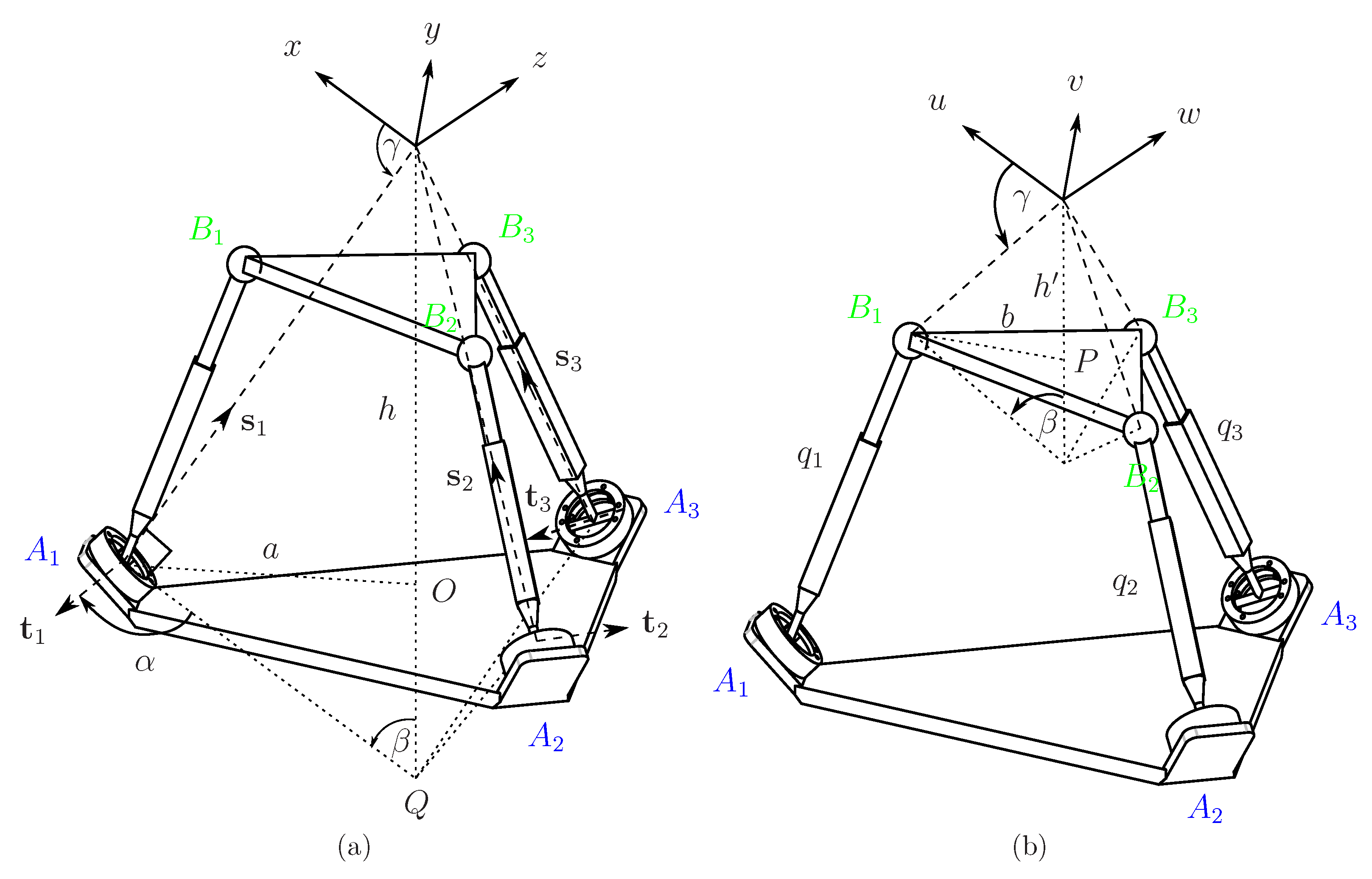
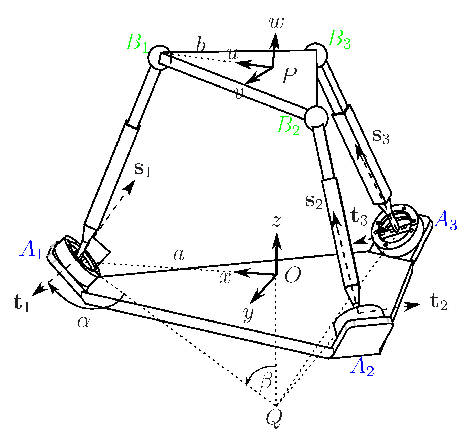
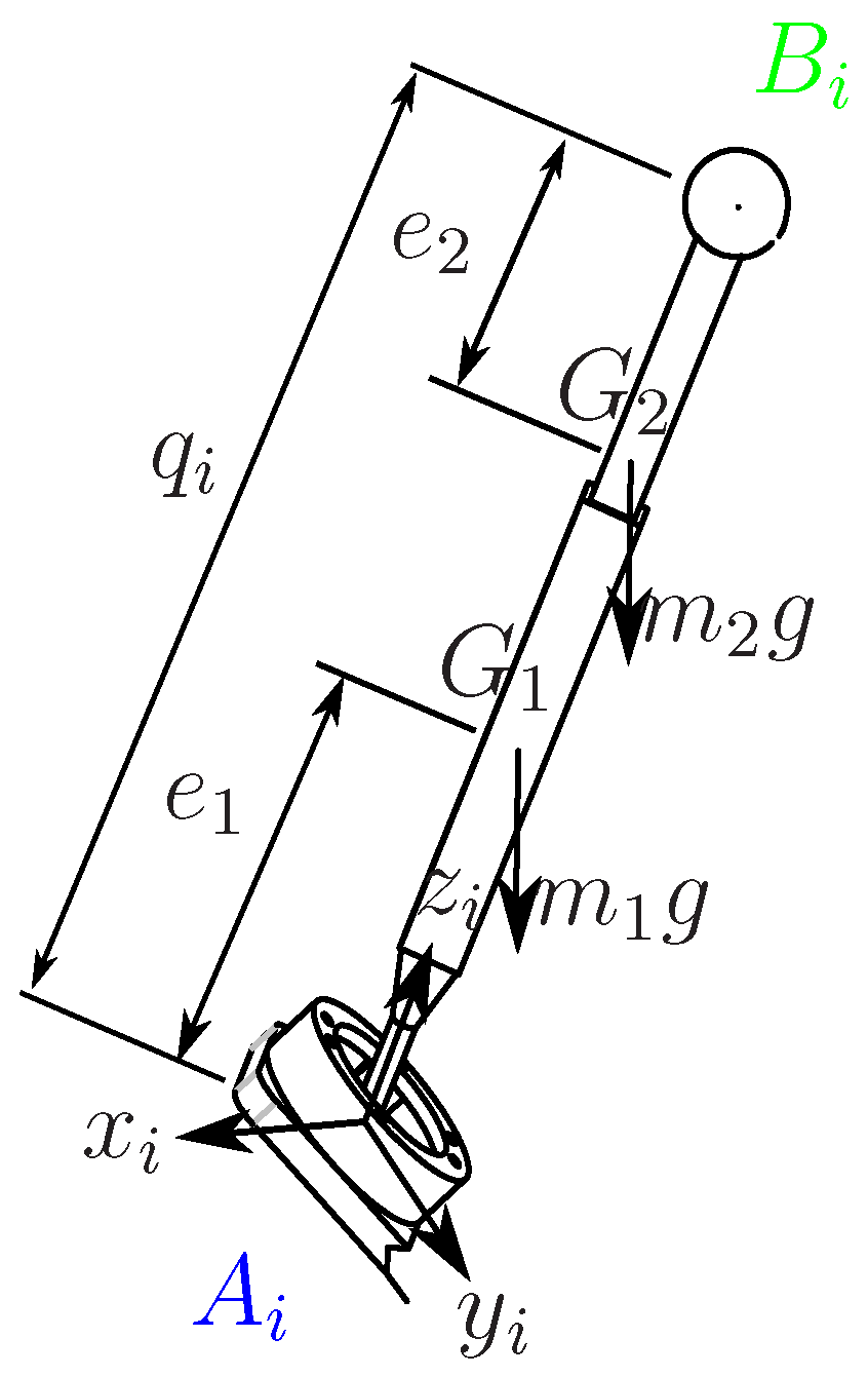
The 3-(rR)PS metamorphic parallel mechanism is depicted in Figure 1 and Figure 2. The (rR), P and S stand for (rR) metamorphic joint, prismatic joint, and spherical joint. The (rR) metamorphic joint consists of two orthogonal revolute joints: the first R-joint performs discrete rotation to alter the direction of R-joint and the R-joint rotates continuously. The geometric description and kinematic problems of the 3-(rR)PS manipulator have been discussed in more detail in [39]. The base and moving platform are equilateral triangles whose vertices are, respectively, denoted by points $A_i$ and $B_i$ of position vectors ${\mathbf{a}}_i$ and ${\mathbf{b}}_i$, $i=1,2,3$. They are connected by three identical (rR)PS kinematic chains, whose prismatic joint is actuated of length $q_i$. The circumradius of the base and moving platform are, respectively, defined by a and b. The origins of the base and moving platform are, respectively, denoted by points O and P.

This mechanism is named metamorphic since it can reconfigure its mobility through an (rR) metamorphic joint [40]. The (rR) metamorphic joint is basically a universal joint that is composed of two perpendicular revolute joints. Their axes are denoted by ${\mathbf{s}}_i$ and ${\mathbf{t}}_i$. The first axis ${\mathbf{s}}_i$ can be independently rotated with an angle $\alpha$ that allows the mechanism to be in different configurations. The second axis ${\mathbf{t}}_i$ moves continuously which contributes to the 3-DOF motions performed by the moving platform. Based on the discrete reconfiguration of $\alpha$, three configurations have been defined in [39] and their dynamics will be analyzed in this paper, namely:

-

Configuration I: $\alpha =0$

-

Configuration II: $0<\alpha <{90}^{\circ }$

-

Configuration III: $\alpha ={90}^{\circ }$

$\angle OQ{A}_i$ is defined by an angle $\beta$ as shown in Figure 1. This angle is a design parameter that will impact the mechanism motion if $\alpha$ is set to be $\alpha \in [0,90)$. However, if $\alpha ={90}^{\circ }$, the mechanism motion is not affected by $\beta$.

At Configuration I, $\alpha$ is null, which makes the axes ${\mathbf{t}}_i$ to intersect at point Q. The fixed coordinate system $(x,y,z)$ and moving coordinate system $(u,v,w)$ are, respectively, located at specific heights h and $h^{\prime }$ from the geometric center of the base and moving platform, as shown in Figure 1.

At Configuration II, the first revolute joint of axis ${\mathbf{s}}_i$ is altered with a value $0<\alpha <{90}^{\circ }$. Thus, the second revolute axes ${\mathbf{t}}_i$ do not intersect and they become skewed. The coordinate system used in this configuration is the same as Configuration I, as shown in Figure 1.

At Configuration III, the axis ${\mathbf{s}}_i$ is rotated about $\alpha ={90}^{\circ }$. It makes the axes of the second revolute joint ${\mathbf{t}}_i$ be coplanar. The design parameter $\beta$ does not have any influence on the mechanism motion, hence $\beta$ will not be used. The fixed coordinate system $(x,y,z)$ and moving coordinate system $(u,v,w)$ are established, respectively, at the geometric center of the base and moving platform, as shown in Figure 2. The expressions of unit vectors ${\mathbf{s}}_i,{\mathbf{t}}_i$ and position vectors ${\mathbf{a}}_i,{\mathbf{b}}_i$ of each configuration are given in [39].

3. Kinematic Analysis

3.1. Inverse Kinematics

The projective coordinate is used to define the position vector of a point in the moving platform and kinematic chains, hence a $4\times 4$ homogeneous transformation matrix T is employed. In this paper, the transformation matrix T is composed of Euler angles $(\varphi ,\theta ,\psi )$ defining the orientations and point-displacement $(x,y,z)$ defining the translations. Transformation matrix T is important for carrying out the coordinate transformation of any point in the moving platform. For each configuration, let the input variables be denoted by a vector $\mathbf{q}$ and the output variables be described by a vector $\mathbf{x}$. Then, the equations of inverse kinematics can be determined, as follows:

$$\mathbf{g}(\mathbf{x},\mathbf{q})=\mathbf{0}$$

(1)

where g is an implicit equation in terms of x and q, and 0 is a zero vector. The mathematical formulation of each component of g is described as follows:

$$g_i:\Vert \mathbf{T}{\mathbf{b}}_i-{\mathbf{a}}_i\Vert -q_i^2=0$$

(2)

By solving Equation (2), the closed-form expression of $q_i$ can be obtained, which is needed for dynamic analysis.

3.2. Velocities

The velocity of any points in the moving platform can be computed by multiplying the position vector of the corresponding point and the velocity matrix $\mathsf{\Omega }$. Therefore, the velocity of geometric center P and vertices $B_i$ can be found by multiplying matrix $\mathsf{\Omega }$ with vectors p and b, as follows:

$$\begin{array}{c}{\mathbf{v}}_p=\mathsf{\Omega }\mathbf{p}\\ {\mathbf{v}}_{b_i}=\mathsf{\Omega }{\mathbf{b}}_i\end{array}$$

(3)

where $\mathbf{p}=\left[p_x{p}_y{p}_z\right]$ and $\mathbf{p}=\left[b_{ix}{b}_{iy}{b}_{iz}\right]$. The velocity matrix $\mathsf{\Omega }$ is obtained by deriving the transformation matrix T with respect to time, as follows:

$$\begin{array}{cc}\mathsf{\Omega }\hfill & =\dot{\mathbf{T}}{\mathbf{T}}^{-1}=\left[\begin{array}{cccc}0& -{\omega }_z& {\omega }_y& v_x\\ {\omega }_z& 0& -{\omega }_x& v_y\\ -{\omega }_y& {\omega }_x& 0& v_z\\ 0& 0& 0& 0\end{array}\right]\hfill \end{array}$$

(4)

Matrix $\mathsf{\Omega }$ is composed of a linear velocity vector ${\mathbf{v}}^T=\left[\begin{array}{ccc}{v}_x& v_y& v_z\end{array}\right]$ and an angular velocity vector ${\omega }^T=\left[\begin{array}{ccc}{\omega }_x& {\omega }_y& {\omega }_z\end{array}\right]$. The angular velocities are obtained from the upper left $3\times 3$ skew-symmetric matrix, which provides helicoidal velocity field of a rigid body.

Figure 3 shows that each prismatic joint is composed of a cylinder and a piston of diameter $d_1$ and $d_2$, respectively. The center of mass is denoted by points $G_1$ and $G_2$ of masses $m_1$ and $m_2$, respectively. The distance from the corresponding center of mass to the edge of cylinder and piston, are, respectively, denoted by $e_1$ and $e_2$. A local coordinate system of (rR)PS leg is established at point $A_i$. The $y_i$ axis and the revolute joint axis ${\mathbf{t}}_i$ are collinear. The $z_i$ is along the leg $A_i{B}_i$. Then, the velocity of point $B_i$ in Equation (3) can be expressed in the leg coordinate system, as ${}^i{\mathbf{v}}_{b_i}$. The linear and angular velocities, ${}^i{\omega }_i$ and ${\dot{q}}_i$, of the i-th leg can be determined from ${}^i{\mathbf{v}}_{b_i}$, as follows:

$$\begin{array}{c}{\displaystyle {}^i{\omega }_i=\frac{1}{e_i}{(}^i{\mathbf{u}}_i{\times }^i{\mathbf{v}}_{b_i})}\hfill \\ {\dot{q}}_i{=}^i{\mathbf{v}}_{b_i}^T{}^i{\mathbf{u}}_i\hfill \end{array}$$

(5)

where ${}^i{\mathbf{u}}_i$ is a unit vector of the i-th leg, as ${}^i{\mathbf{u}}_i^T=\left[\begin{array}{ccc}0& 0& 1\end{array}\right]$. The velocities of the center of mass $G_1$ and $G_2$ can be determined in terms of the linear and angular velocities, as follows:

$$\begin{array}{c}{}^i{\mathbf{v}}_{G_{1i}}=e_1{(}^i{\omega }_i{\times }^i{\mathbf{u}}_i)\hfill \\ {}^i{\mathbf{v}}_{G_{2i}}=(q_i-e_2){(}^i{\omega }_i{\times }^i{\mathbf{u}}_i){+}^i{\dot{q}}_i{}^i{\mathbf{u}}_i\hfill \end{array}$$

(6)

and the velocities of center of mass $G_i$ and $G_2$ should be transformed into the fixed coordinate system, as ${\mathbf{v}}_{G_{1i}}$ and ${\mathbf{v}}_{G_{2i}}$.

3.3. Singularities

The vanishing condition of the determinant of direct Jacobian and inverse Jacobian correspond to Type 2 and Type 1 singularities, respectively [9]. In what follows, we will consider only Type 2 singularity (actuation singularity) and the singularity surface/curve will be represented in Cartesian space within the mechanism workspace. In the singular configuration, the actuators cannot control the velocity of the moving platform, thus it loses the ability to transmit motion and forces.

By taking the time derivative of Equation (1), the Jacobian matrices defining the relationship of input–output velocities ($\dot{\mathbf{q}}$ and $\dot{\mathbf{x}}$, respectively) are obtained, as follows:

$$\mathbf{A}\dot{\mathbf{x}}+\mathbf{B}\dot{\mathbf{q}}=\mathbf{0}$$

(7)

where A and B are, respectively, called direct Jacobian and inverse Jacobian. They are expressed as follows:

$$\mathbf{A}=\left(\frac{\partial \mathbf{g}}{\partial \mathbf{x}}\right)\mathrm{and}\mathbf{B}=\left(\frac{\partial \mathbf{g}}{\partial \mathbf{q}}\right)$$

If the rank of Jacobian matrices A and B degenerate, it indicates that the mechanism is subjected to Type 2 and Type 1 singularities, respectively. In this paper, only Type 2 singularity is investigated, and it can be identified when the determinant of matrix A vanishes, as follows:

$$\det \left(\mathbf{A}\right)=0$$

(8)

Direct Jacobian A becomes rank-deficient by at least one which means at least two columns are linearly dependent. A non-zero vector n exists, which is defined as the null space of A, and their relationship can be written as:

$$\mathbf{A}\mathbf{n}={\mathbf{n}}^T{\mathbf{A}}^T=\mathbf{0}$$

(9)

The null space vector n provides the direction of uncontrollable motion performed by the moving platform in a singular position.

4. Dynamic Models for Crossing Singularities

The dynamic models used in this paper are based on the Lagrangian formulation, which can be written as follows:

$$\tau ={\mathbf{W}}_b-\mathbf{B}\lambda ,{\mathbf{W}}_b=\frac{d}{dt}\left(\frac{\partial L}{\partial \dot{\mathbf{q}}}\right)-\frac{\partial L}{\partial \mathbf{q}}$$

(10a)

$$\mathbf{A}\lambda ={\mathbf{W}}_a,{\mathbf{W}}_a=\frac{d}{dt}\left(\frac{\partial L}{\partial \dot{\mathbf{x}}}\right)-\frac{\partial L}{\partial \mathbf{x}}$$

(10b)

where A and B are Jacobian matrices derived from Equation (7), $\lambda$ is the Lagrange multiplier, and L denotes the Lagrangian function. The Lagrangian function is defined as the difference between total kinetic energy (K) and potential energy (U) of the legs and moving platform, as:

$$L=K-U$$

(11)

The height is described as a distance from any desired points to origin O. Frictions and elasticity of the system are omitted; therefore, the potential energy of this mechanism can be described as follows:

$$U=m_{p}g{h}_p+\sum _{i=1}^3(m_{1}g{h}_{G_{1i}}+m_{2}g{h}_{G_{2i}})$$

(12)

where $h_p$, $h_{G_{1i}}$, $h_{G_{2i}}$ are the vertical distances of moving platform center of mass P, $G_{1i}$ and $G_{2i}$, respectively. The kinetic energy can be derived as follows:

$$K=\frac{1}{2}{m}_p{\mathbf{v}}_p^2+\frac{1}{2}{\omega }_p^T{\mathbf{I}}_p{\omega }_p+\sum _{i=1}^3\left(\frac{1}{2}{m}_1{\mathbf{v}}_{G_{1i}}^2+\frac{1}{2}{m}_2{\mathbf{v}}_{G_{2i}}^2+\frac{1}{2}{\omega }_i^T({\mathbf{I}}_{G_{1i}}+{\mathbf{I}}_{G_{2i}}){\omega }_i\right)$$

(13)

For a prescribed trajectory $\mathbf{x}\left(t\right)$ passing through a singularity, the determinant of Jacobian $\mathbf{A}$ is null. Then, input forces exerted by the actuators to the system become numerically infinite. Consequently, the mechanism is not able to continue the task along the prescribed trajectory and is locked in such a singular position. By taking dot-product of both sides of Equation (10b) with the null space vector n, the consistency condition of the dynamic model is derived as follows:

$${\mathbf{n}}^T{\mathbf{A}}^T\lambda ={\mathbf{n}}^T{\mathbf{W}}_a=\mathbf{0}$$

(14)

It shows that the wrench ${\mathbf{W}}_a$ and Jacobian A should be reciprocal to the uncontrollable motion n in the presence of the singularity. Equation (14) is the first condition to fulfil for the mechanism to pass through singularity based on [33,34]. However, this condition is not sufficient to guarantee the input forces to be finite when the determinant of A is null.

At singular configuration, Jacobian A is not invertible because its determinant is null. Consequently, the input forces of parallel mechanisms tend towards infinity and cannot be determined. Based on [32,38], this singularity can be removed by imposing the indeterminate form into our dynamic models, then L’H$\widehat{\mathrm{o}}$pital’s rule can be applied. L’H$\widehat{\mathrm{o}}$pital’s rule allows us to use basic calculus to solve the singularity. L’H$\widehat{\mathrm{o}}$pital’s rule implies that the limit of an indeterminate function is equal to the limit of the derivatives of those functions. Let $f\left(x\right)$ and $g\left(x\right)$ be continuous functions on an interval consisting of $x=c$, such that two indeterminate forms are obtained as follows:

1.

${lim}_{x\to c}{\displaystyle \frac{f\left(x\right)}{g\left(x\right)}}$ is type ${\displaystyle \frac{0}{0}}$ if ${lim}_{x\to c}f\left(x\right)={lim}_{x\to c}g\left(x\right)=0$

2.

${lim}_{x\to c}{\displaystyle \frac{f\left(x\right)}{g\left(x\right)}}$ is type ${\displaystyle \frac{\infty }{\infty }}$ if ${lim}_{x\to c}f\left(x\right)={lim}_{x\to c}g\left(x\right)=\infty$

Let the Lagrange multiplier $\lambda$ from Equation (10b) be written in terms of time t, as follows:

$$\lambda \left(t\right)={\left(\mathbf{A}\left(t\right)\right)}^{-1}{\mathbf{W}}_a\left(t\right)$$

(15)

The inverse of Jacobian $\mathbf{A}\left(t\right)$ can be represented as a multiplication of adjoint of $\mathbf{A}\left(t\right)$ by the inverse of determinant ${\displaystyle \frac{1}{\det \left(\mathbf{A}\right(t\left)\right)}}$, as follows:

$$\lambda \left(t\right)=\frac{1}{\det \left(\mathbf{A}\right(t\left)\right)}\mathrm{adj}\left(\mathbf{A}\left(t\right)\right){\mathbf{W}}_a\left(t\right)$$

(16)

In what follows, the numerator and denominator of $\lambda \left(t\right)$ will be denoted by $\sigma \left(t\right)=\mathrm{adj}\left(\mathbf{A}\left(t\right)\right){\mathbf{W}}_a\left(t\right)$ and $\delta \left(t\right)=\det \left(\mathbf{A}\right(t\left)\right)$, respectively. Then, the limit can be applied as the time t approaches singularity time $t_s$, as:

$$\underset{t\to t_s}{lim}\lambda \left(t\right)=\underset{t\to t_s}{lim}\frac{\sigma \left(t\right)}{\delta \left(t\right)}$$

(17)

when $t=t_s$, the denominator is null, i.e., $\delta \left(t_s\right)=0$ and Equation (17) becomes indefinite. Such a limit can be deduced by applying L’H$\widehat{\mathrm{o}}$pital’s rule if and only if one of the indeterminate forms is satisfied, namely ${lim}_{t\to t_s}\sigma \left(t\right)$ and ${lim}_{t\to t_s}\delta \left(t\right)$ are both equal to zero or infinity. The indeterminate form of type ${\displaystyle \frac{0}{0}}$ at $t=t_s$ is used in this paper because by imposing both numerator and denominator zero, the magnitude of velocity, acceleration, and jerk at singularity can be computed. Hence, Equation (17) can be represented as:

$$\frac{\sigma \left(t_s\right)}{\delta \left(t_s\right)}=\frac{0}{0}$$

(18)

Since $\delta \left(t_s\right)=0$ is always true, then $\sigma \left(t_s\right)$ will be zero if one of the following statements holds:

1.

${\mathbf{W}}_a\left(t_s\right)=0$

2.

$\mathrm{adj}\left(\mathbf{A}\left(t_s\right)\right){\mathbf{W}}_a\left(t_s\right)=0$

Equation (18) becomes the second condition to achieve in order for the mechanism to pass through the singularity. As the indeterminate form is now fulfilled, the first time derivative of L’H$\widehat{\mathrm{o}}$pital’s rule can be applied, as:

$$\underset{t\to ts}{lim}\lambda \left(t\right)=\underset{t\to ts}{lim}\frac{{\sigma }^{\prime }\left(t\right)}{{\delta }^{\prime }\left(t\right)}$$

(19)

In this paper, the third condition is proposed by imposing ${lim}_{t\to ts}{\displaystyle \frac{{\sigma }^{\prime }\left(t\right)}{{\delta }^{\prime }\left(t\right)}}$ to be an indeterminate form of type ${\displaystyle \frac{0}{0}}$, such that:

$$\frac{{\sigma }^{\prime }\left(t_s\right)}{{\delta }^{\prime }\left(t_s\right)}=\frac{0}{0}$$

(20)

therefore, the second time derivative of L’H$\widehat{\mathrm{o}}$pital’s rule should be computed, as follows:

$$\underset{t\to ts}{lim}\lambda \left(t\right)=\underset{t\to ts}{lim}\frac{{\sigma }^{″}\left(t\right)}{{\delta }^{″}\left(t\right)}$$

(21)

The first, second, and third conditions defined in Equations (14), (18) and (20), respectively, will introduce not only velocity and acceleration but also jerk in the system. Hence, their magnitudes should be carefully planned in the neighborhood of singularity. The next crucial task is to generate a trajectory that ensures the mechanism satisfies all three conditions, such that the mechanism is able to effortlessly pass through the singularity. By establishing the positions, velocities, accelerations, and jerks at the initial, final, and singular configurations, the 11th-degree polynomial is used for trajectory planning because they provide smooth and continuous efforts $\tau$.

5. Results and Discussions

Based on [33,34], the mechanism can pass through singularities by respecting only one condition written in Equation (14). The uncontrollable motion defined by the null space n should be reciprocal to the wrench ${\mathbf{W}}_a$. It indicates that the wrench ${\mathbf{W}}_a$ in the given singular position should be orthogonal to the gained motion n. This condition is not sufficient to allow the mechanism to pass through the singularity without infinite forces/torques. Thus, a second condition proposed in [38] should be also fulfilled, namely the indeterminate form where the product of adjoint A and the wrench ${\mathbf{W}}_a$ should vanish as in Equation (18). This vanishing condition can be solved using L’H$\widehat{\mathrm{o}}$pital’s rule. The third condition is employed in this paper, namely the second indeterminate form as in Equation (20). All three conditions are the unified solution for Configurations I, II, and III. The detailed computational results will be confirmed by the ADAMS simulations.

Table 1. Properties of the mechanism.

Properties	Value	Unit
Circumradius of Base $\left(a\right)$	0.25	m
Circumradius of Moving Platform $\left(b\right)$	0.125	m
Mass of Moving Platform $\left(m_p\right)$	1.5	kg
Thickness of Moving Platform $\left(t_p\right)$	0.01	m
Mass of Piston $\left(m_1\right)$	0.166	kg
Mass of Cylinder $\left(m_2\right)$	0.166	kg
Centre of Piston Gravity $\left(e_1\right)$	0.09	m
Central of Cylinder Gravity $\left(e_2\right)$	0.1	m
Diameter of Piston $\left(d_1\right)$	0.01	m
Diameter of Cylinder $\left(d_2\right)$	0.01 + 0.005	m
Gravity (g)	10	kgm/s${}^2$
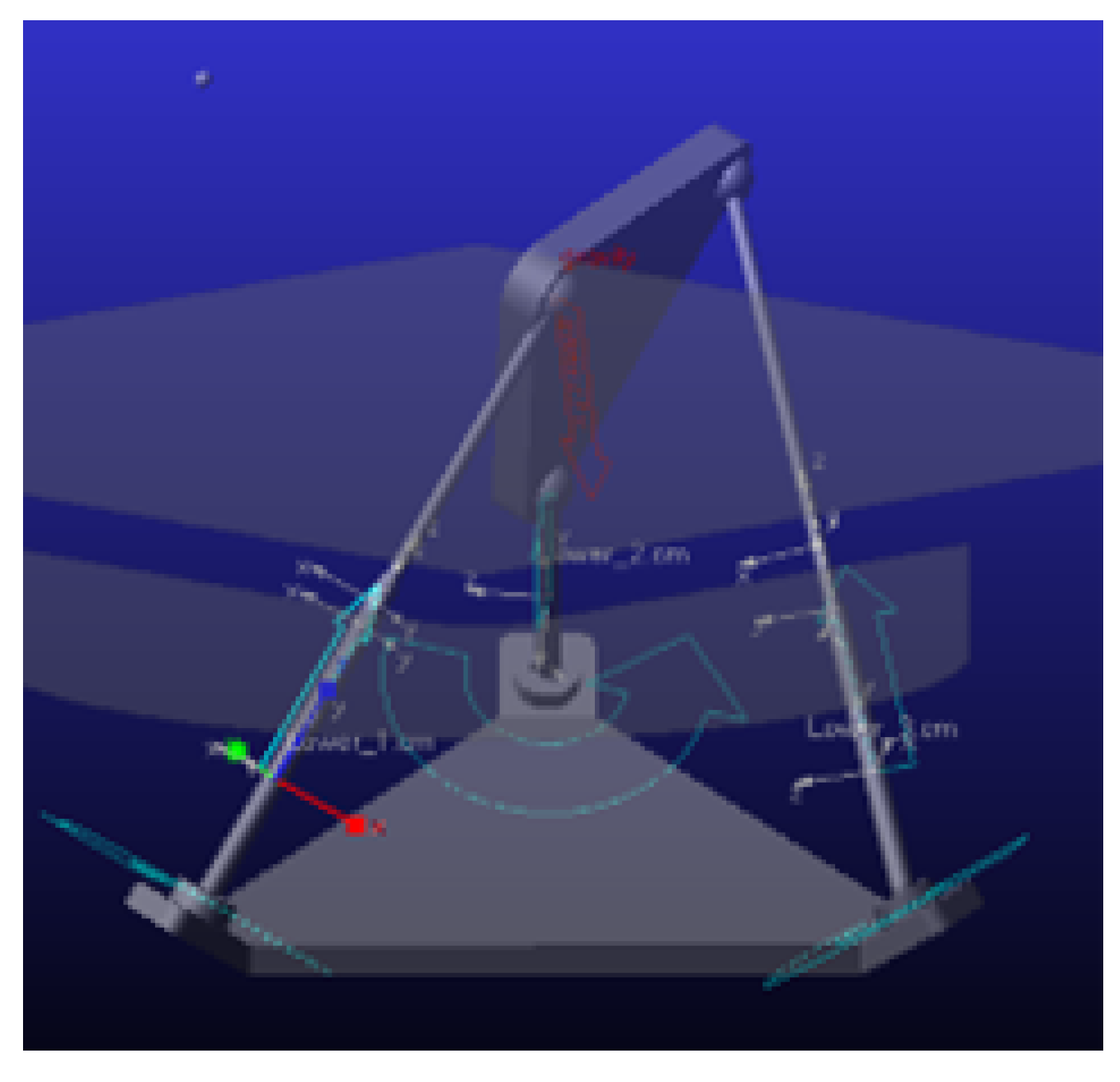
Material	Aluminum

describes the values of design parameters applied for executing the computation in Maple software. These values are also implemented to create the CAD model in Fusion360 used for running the ADAMS simulation. The ADAMS multibody model is shown in Figure 4. The computer used in this work has the following technical specifications: Processor core-i7 gen 12, VGA GeForce GTX 1650 super, RAM 32 GB, SSD 512 GB. In the following analysis, the numerical results and ADAMS simulations may show slight differences due to several factors, i.e., the technique of the initial position of the robot is defined during the simulation, and the robot CAD model is generated from different software which may consequently affect the coordinate location in ADAMS.

5.1. Configuration I: $\alpha =0^{\circ }$

The motion performed by Configuration I is a 3-DOF rotational motion which is not about a fixed point or a fixed axis. This motion is described by the output variables $\mathbf{x}=\left[\begin{array}{ccc}\varphi & \theta & \psi \end{array}\right]$. For a given value of $(\varphi ,\theta ,\psi )$, the geometric center of moving platform will be displaced by $({\delta }_x,{\delta }_y,{\delta }_z)$ as expressed by the transformation matrix ${\mathbf{T}}_I$ in Equation (22). The design parameter $\beta$ also has a great influence on the motion which eventually reshapes the mechanism workspace.

$${\mathbf{T}}_{\mathrm{I}}=\left[\begin{array}{cccc}{c}_{\varphi }{c}_{\psi }-s_{\varphi }{c}_{\theta }{s}_{\psi }& -c_{\varphi }{s}_{\psi }-s_{\varphi }{c}_{\theta }{c}_{\psi }& s_{\varphi }{s}_{\theta }& {\delta }_x\\ s_{\varphi }{c}_{\psi }+c_{\varphi }{c}_{\theta }{s}_{\psi }& -s_{\varphi }{s}_{\psi }+c_{\varphi }{c}_{\theta }{c}_{\psi }& -c_{\varphi }{s}_{\theta }& {\delta }_y\\ s_{\theta }{s}_{\psi }& s_{\theta }{c}_{\psi }& c_{\theta }& {\delta }_z\\ 0& 0& 0& 1\end{array}\right]$$

(22)

where

$$\begin{array}{ccc}{\delta }_x={\displaystyle \frac{A_1{c}_{\beta }^2+B_1{s}_{\beta }{c}_{\beta }+C_1}{s_{\beta }^2{c}_{\beta }^2}}\hfill & {\delta }_y={\displaystyle \frac{A_2{c}_{\beta }^2+B_2{s}_{\beta }{c}_{\beta }+C_2}{s_{\beta }^2{c}_{\beta }^2}}\hfill & {\delta }_z={\displaystyle \frac{A_3{c}_{\beta }^2+B_3{s}_{\beta }{c}_{\beta }+C_3}{s_{\beta }^2{c}_{\beta }^2}}\hfill \end{array}$$

where $A_i,B_i,C_i$ are polynomial coefficients in terms of output variables $(\varphi ,\theta ,\psi )$. Its mathematical expressions are quite lengthy and will not be shown in this paper.

After performing the coordinate transformation using matrix ${\mathbf{T}}_I$, the inverse kinematics can be obtained by applying Equation (22), as: $\mathbf{g}=\langle g_1,g_2,g_3\rangle$. These equations are derived with respect to time to compute direct-inverse Jacobians. The singularity curves/surfaces are then determined by computing the zero set of the determinant of Jacobian A.

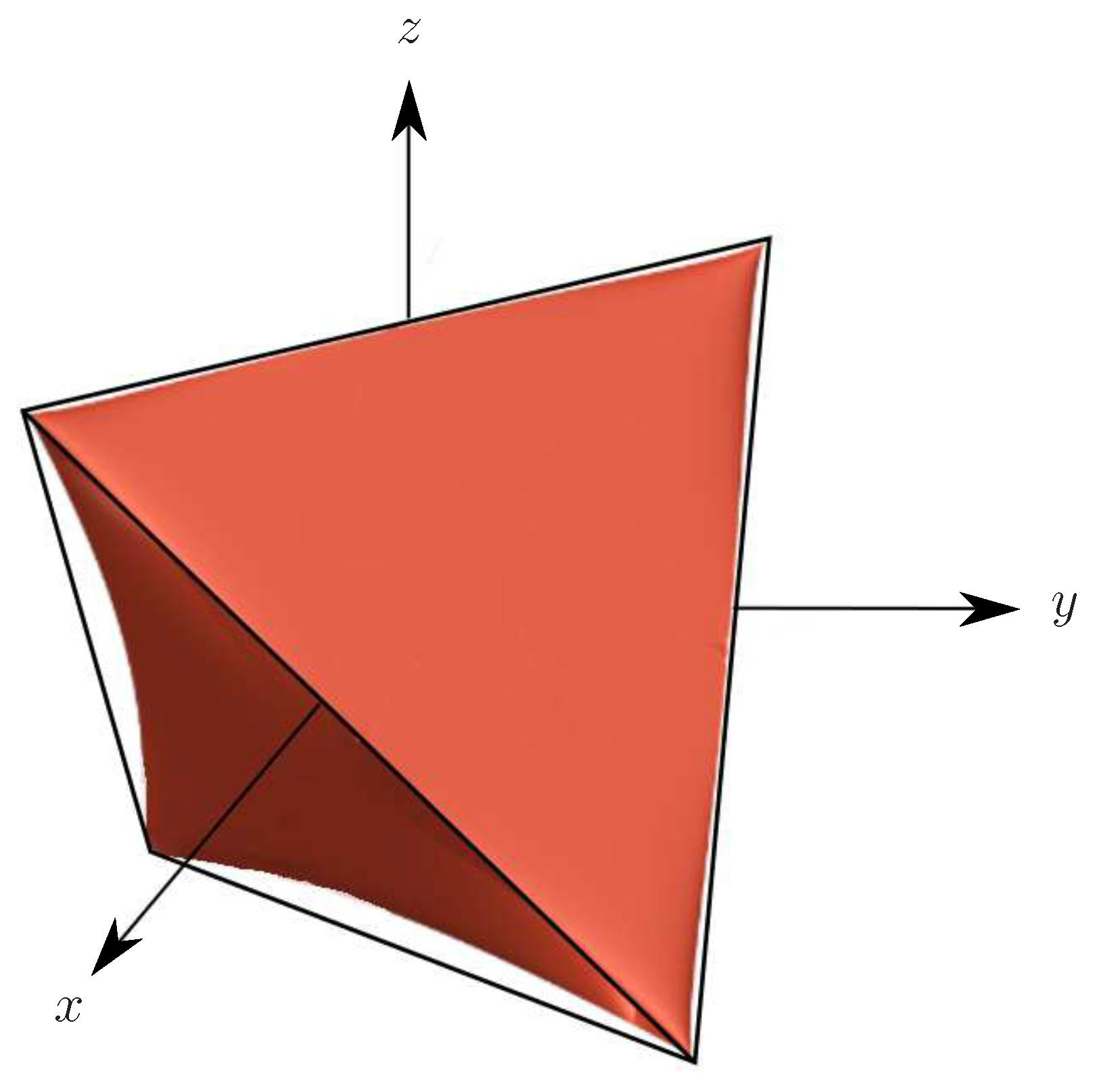
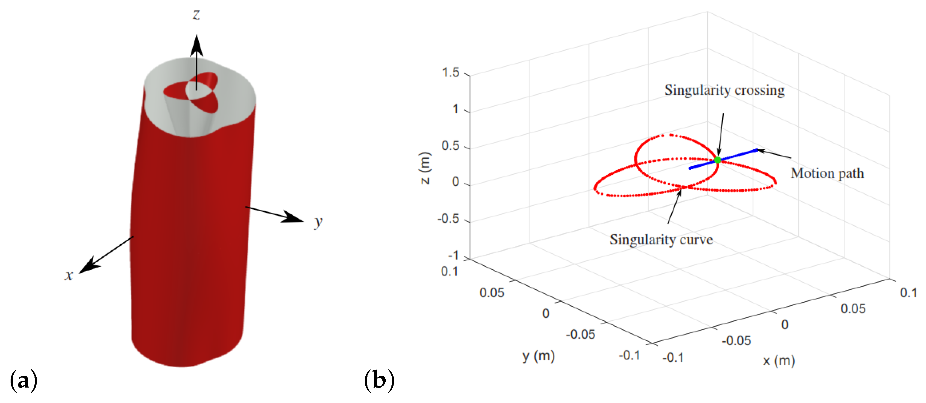
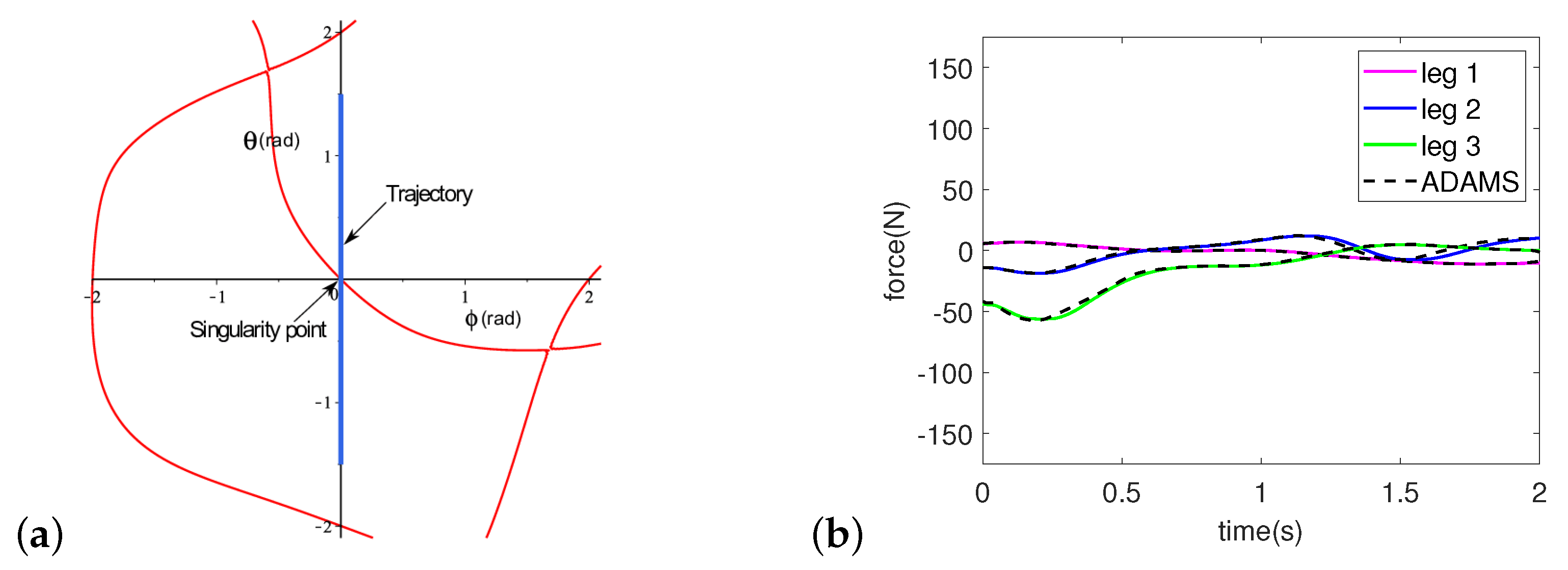
Let $\beta$ be assigned by $\beta =54.7^{\circ }$, thus the revolute joints ${\mathbf{t}}_i$ are orthogonal. Based on [39], its workspace is bounded by a tetrahedron. Therefore, the singularity surface is plotted inside its tetrahedron as shown in Figure 5.

A path is generated to be followed by the moving platform such that it crosses a point in the singularity surface in Figure 5. Let this path be defined by a single parameter $\theta$, thus the moving platform undergoes 1-DOF motion parametrized by $\theta$ the other two output variables as: $\varphi =\psi =0$. The Jacobians A and B become:

$$\begin{array}{c}\varphi =\psi =0\hfill \\ \mathbf{A}=3\left[\begin{array}{ccc}8s_{\theta }-2s_{2\theta }& 4-2c_{\theta }& -c_{2\theta }-1+4c_{\theta }-s_{2\theta }+4s_{\theta }\\ -c_{2\theta }-1+4c_{\theta }-s_{2\theta }+4s_{\theta }& -2c_{\theta }& -2\\ 2c_{2\theta }+4s_{\theta }-4c_{\theta }& 2s_{\theta }& 0\end{array}\right]\hfill \\ \mathbf{B}=-256\left[\begin{array}{ccc}{q}_1& 0& 0\\ 0& q_2& 0\\ 0& 0& q_3\end{array}\right]\hfill \end{array}$$

(23)

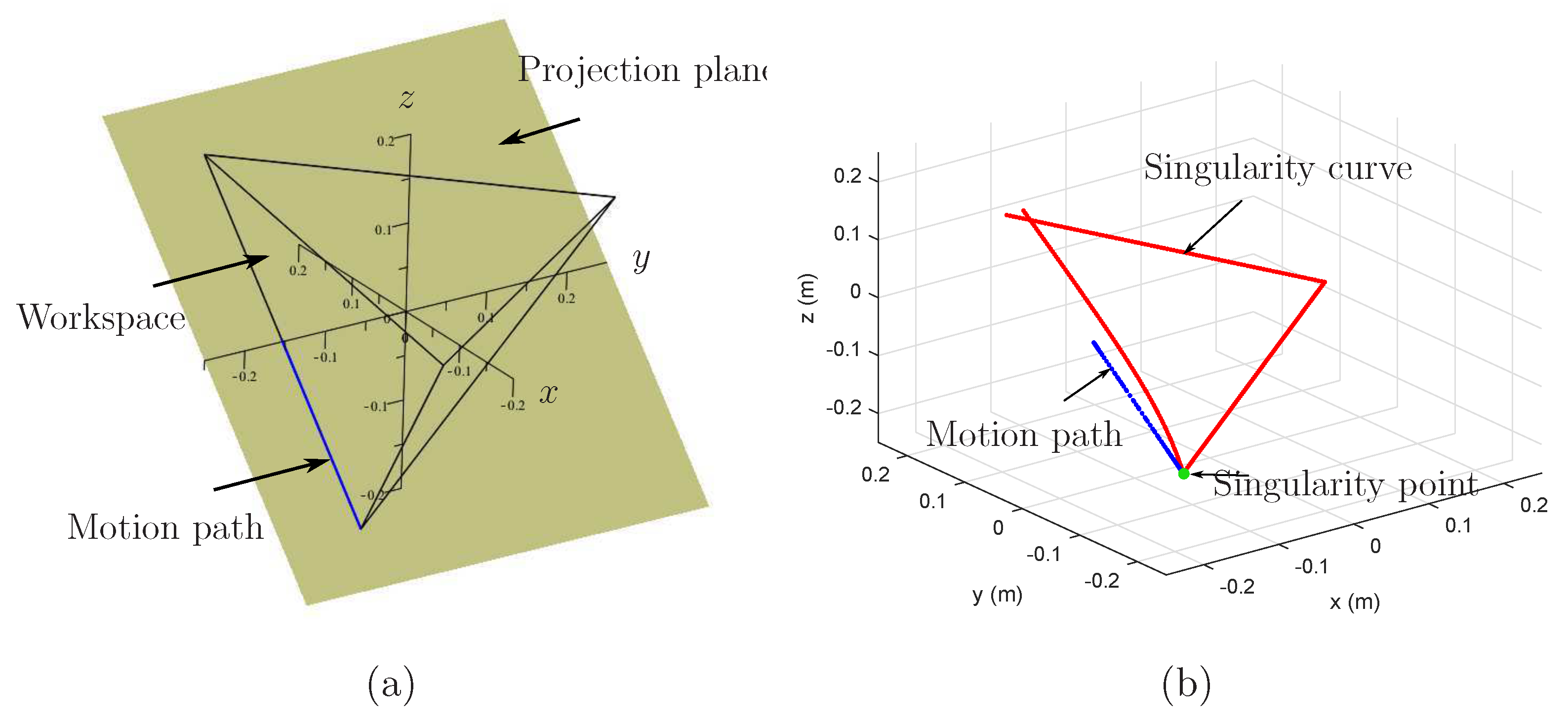
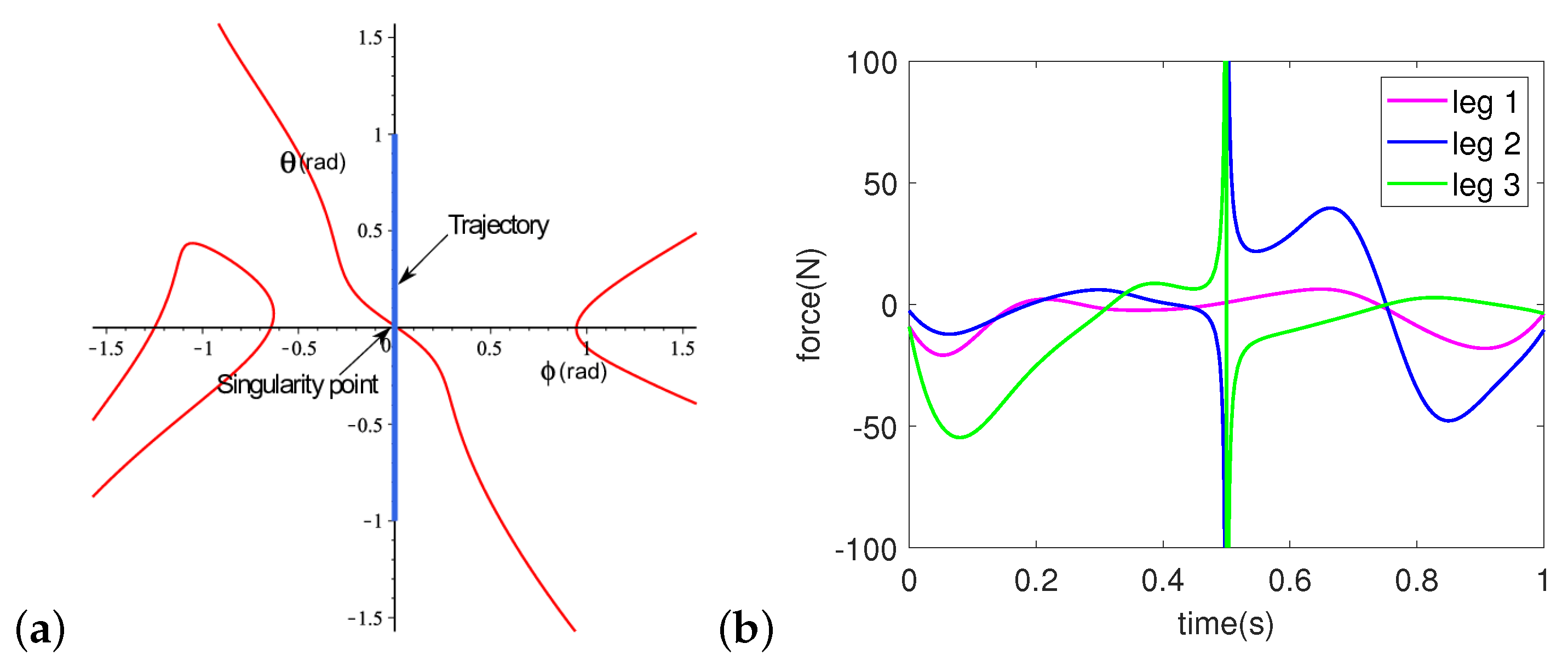
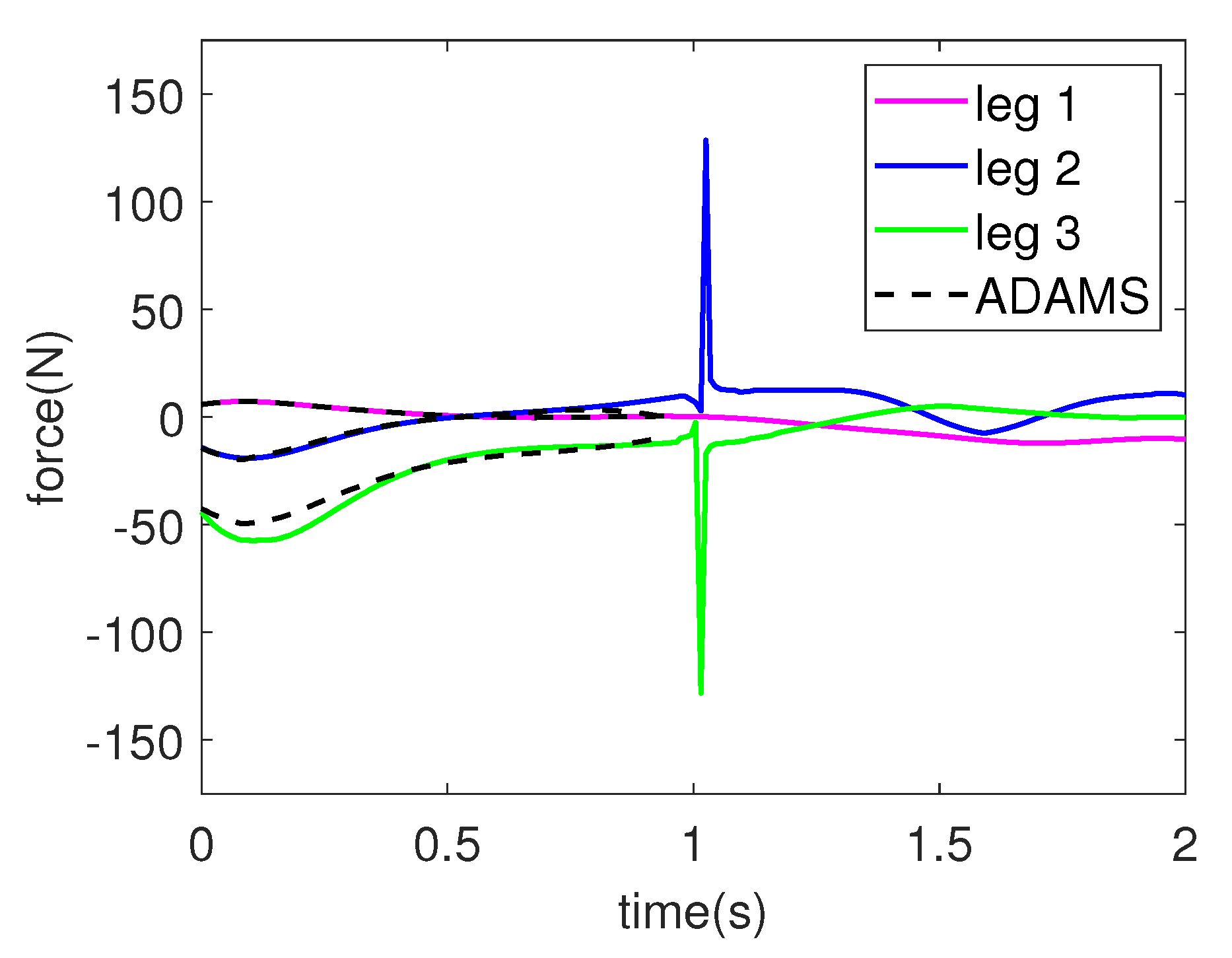
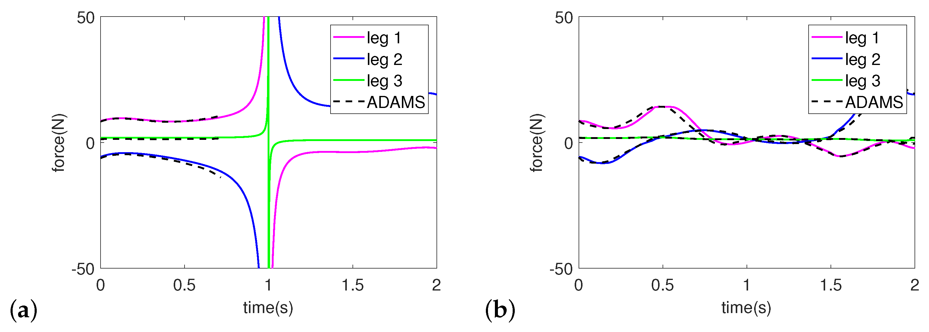
A projection plane $y-z=0$ is created to better visualize the motion path and singularity curve inside the tetrahedron, as shown in Figure 6a. On this projection plane, the singularity curve crossed by the motion path at $\theta =0$ is depicted in Figure 6b. The inverse dynamics during a given task are computed and the motor force distribution is depicted in Figure 7. The motor force of the first leg is finite but the forces of the other two legs are infinite at $t=1s$. 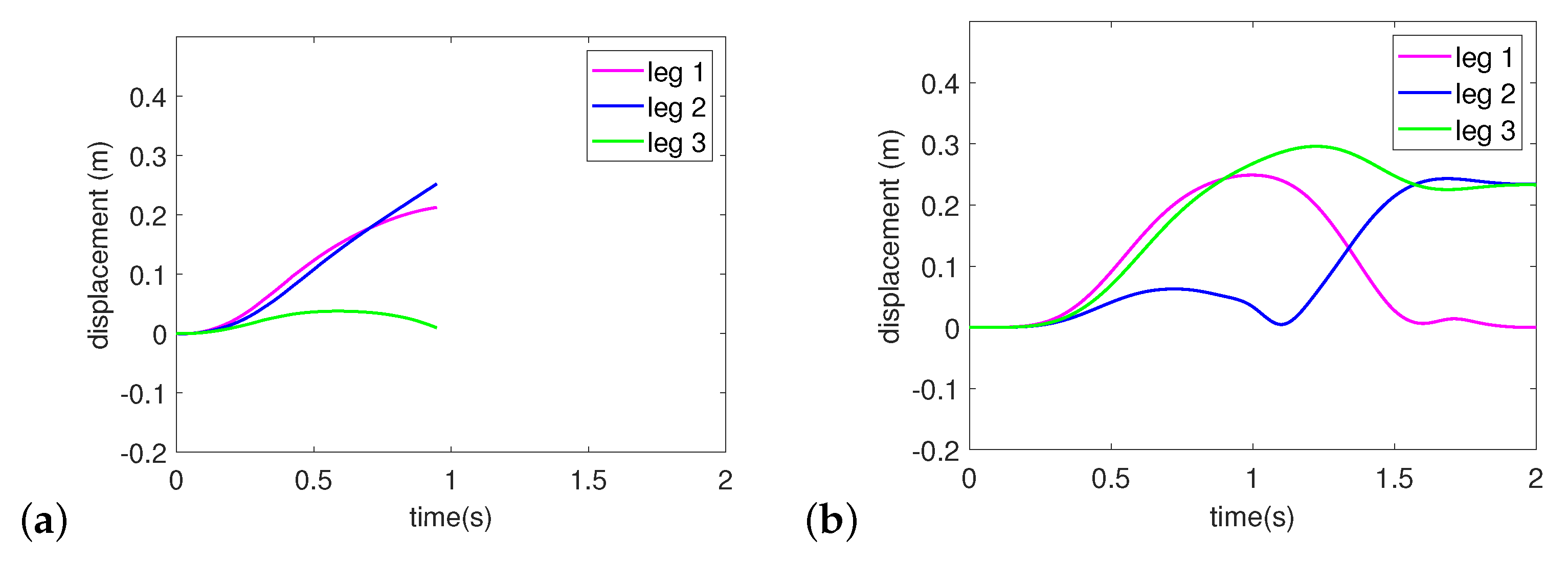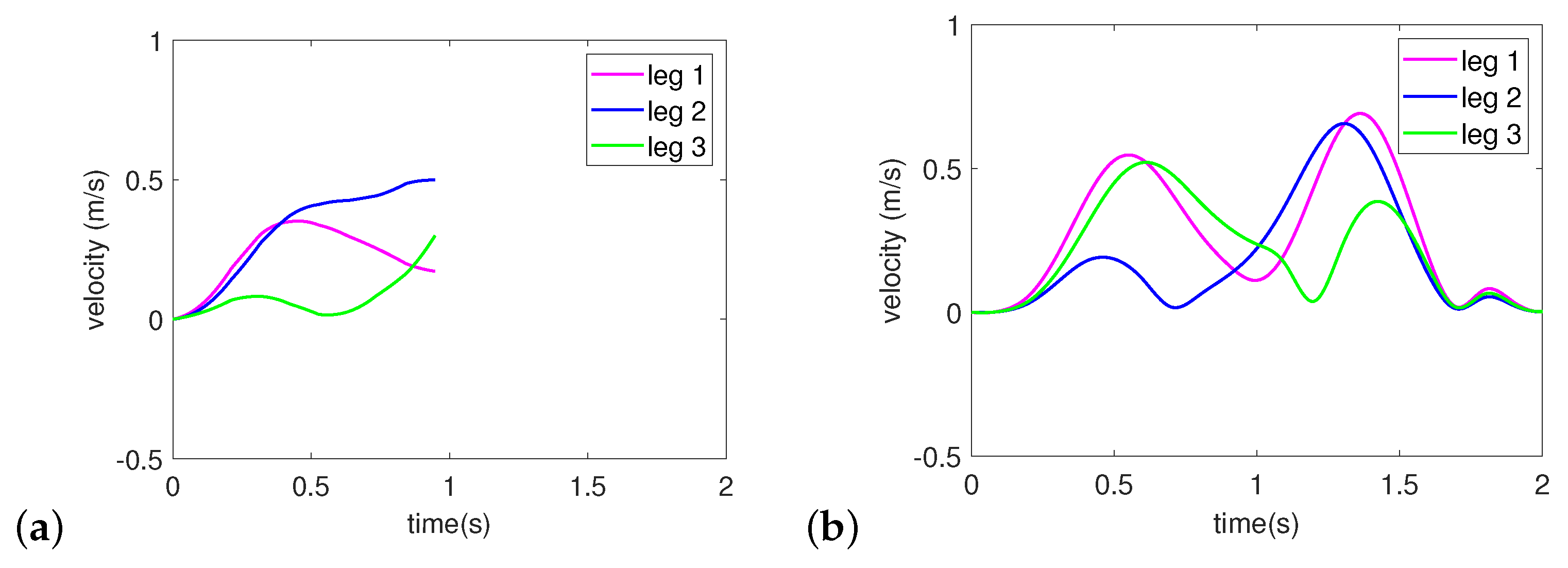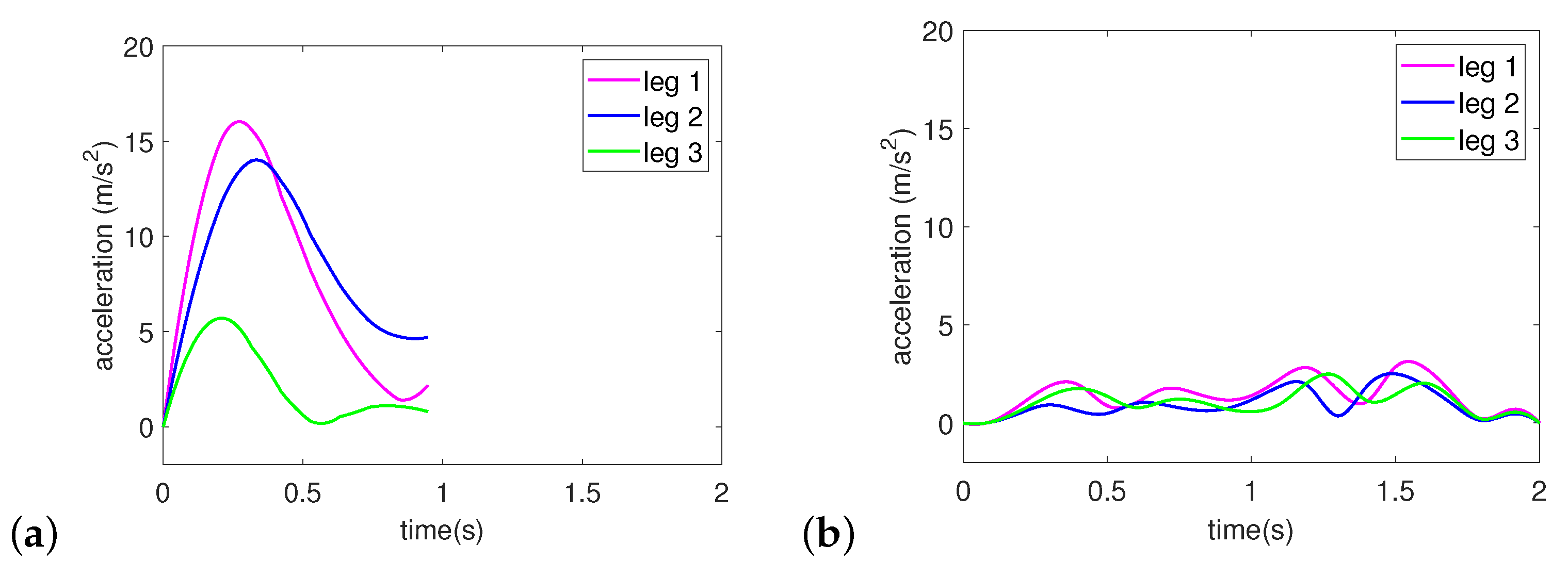The actuator joint displacements, velocities, and accelerations are, respectively, shown in Figure 8a, Figure 9a and Figure 10a. Those graphs are discontinued as the mechanism reaches singularities.

At the singularity, Jacobian A becomes rank-deficient by one and the gained motion can be obtained by computing the null space. This gained motion is an infinitesimal rotation, as follows:

$$\mathbf{n}=\left[\begin{array}{c}0\\ -1\\ 1\end{array}\right]$$

(24)

By respecting the first, second, and third conditions in Equations (14), (18) and (20), respectively; velocity, acceleration, and jerk can be enumerated. Let the motion duration last for 2 s and the singularity occur at t = 1 s. Then, the boundary conditions during the initial ($t_i$), singular ($t_s$) and final ($t_f$) positions can be determined, as follows:

$$\begin{array}{cccc}\theta \left(t_i\right)=-{90}^{\circ }\hfill & \dot{\theta }\left(t_i\right)=0\hfill & \ddot{\theta }\left(t_i\right)=0\hfill & \stackrel{⃛}{\theta }\left(t_i\right)=0\hfill \\ \theta \left(t_s\right)=0^{\circ }\hfill & \dot{\theta }\left(t_s\right)=2.46\hfill & \ddot{\theta }\left(t_s\right)=3.86\hfill & \stackrel{⃛}{\theta }\left(t_s\right)=-5.19\hfill \\ \theta \left(t_f\right)={90}^{\circ }\hfill & \dot{\theta }\left(t_f\right)=0\hfill & \ddot{\theta }\left(t_f\right)=0\hfill & \stackrel{⃛}{\theta }\left(t_f\right)=0\hfill \end{array}$$

(25)

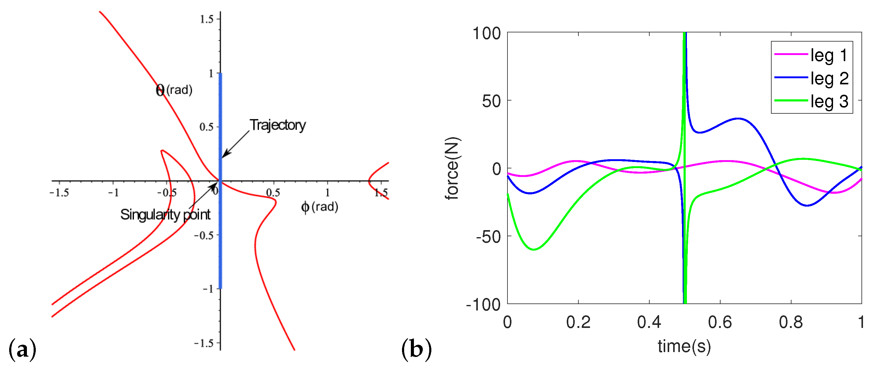
then the 11th-degree polynomial trajectory to be followed by the moving platform can be generated, as follows:

$$\theta \left(t\right)=-1.57+74t^4-284t^5+480t^6-450t^7+260t^8-86t^9+15.9t^{10}-1.30t^{11}$$

(26)

The 11th-degree trajectory defined in Equation (26) crosses the singularity at $\theta =0$, as shown in Figure 11a. Upon fulfilling the first, second, and third conditions, the actuator displacements, velocities, accelerations, and forces are finite as, respectively, shown in Figure 8b, Figure 9b, Figure 10b and Figure 11b, meaning that the moving platform can swiftly pass through singularity. The singularity curve in the orientation workspace and inverse dynamics of $\beta ={60}^{\circ }$ are solved too for comparisons, as shown in Figure 12. More effort is required by the motors when $\beta ={60}^{\circ }$. 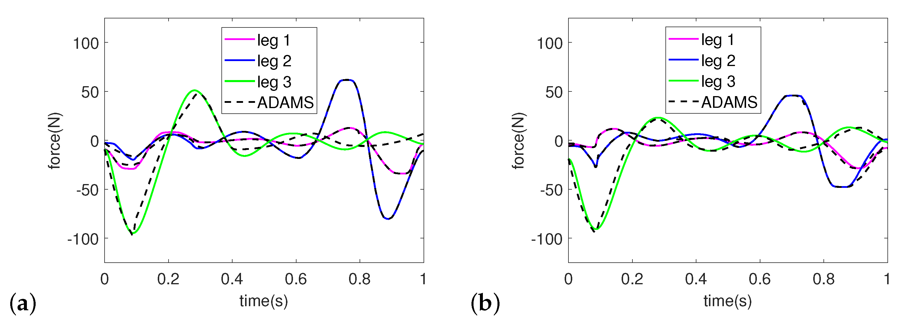The ADAMS simulation has been used to corroborate the results of dynamic analysis. The Mean Absolute Errors between the numerical results and the ADAMS simulation are 0.211, 0.518, and 0.891 for, respectively, the 1st, 2nd, and 3rd leg.

5.2. Configuration II: $0^{\circ }<\alpha <{90}^{\circ }$

In Configuration II, the revolute axes ${\mathbf{t}}_i$ are skewed since the design parameter $\alpha$ is no longer 0. The motion performed by the moving platform is a 3-DOF rotational motion not about a fixed axis or a fixed point. The output variables of this motion are $\mathbf{x}=\left[\begin{array}{c}\varphi ,\theta ,\psi \end{array}\right]$. The motion seems identical to the one belonging to Configuration I. However, the displacement of the geometric center defined by $({\Delta }_x,{\Delta }_y,{\Delta }_z)$ in matrix ${\mathbf{T}}_{II}$ gives an entirely different motion. The workspace of Configuration II is a distorted tetrahedron which has been thoroughly discussed in [39].

$${\mathbf{T}}_{\mathrm{II}}=\left[\begin{array}{cccc}{c}_{\varphi }{c}_{\psi }-s_{\varphi }{c}_{\theta }{s}_{\psi }& -c_{\varphi }{s}_{\psi }-s_{\varphi }{c}_{\theta }{c}_{\psi }& s_{\varphi }{s}_{\theta }& {\Delta }_x\\ s_{\varphi }{c}_{\psi }+c_{\varphi }{c}_{\theta }{s}_{\psi }& -s_{\varphi }{s}_{\psi }+c_{\varphi }{c}_{\theta }{c}_{\psi }& -c_{\varphi }{s}_{\theta }& {\Delta }_y\\ s_{\theta }{s}_{\psi }& s_{\theta }{c}_{\psi }& c_{\theta }& {\Delta }_z\\ 0& 0& 0& 1\end{array}\right]$$

(27)

where

$$\begin{array}{c}{\Delta }_x={\displaystyle \frac{A_1{c}_{\beta }^2+B_1{s}_{\beta }{c}_{\beta }+C_1{c}_{\alpha }^3+D_1{c}_{\alpha }^2+E_1{c}_{\alpha }+F_1{s}_{\alpha }}{(3s_{\beta }^2{c}_{\alpha }^2-s_{\alpha }^2)c_{\beta }^2{c}_{\alpha }}}\hfill \\ {\Delta }_y={\displaystyle \frac{A_2{c}_{\beta }^2+B_2{s}_{\beta }{c}_{\beta }+C_2{c}_{\alpha }^3+D_2{c}_{\alpha }^2+E_2{c}_{\alpha }+F_2{s}_{\alpha }}{(3s_{\beta }^2{c}_{\alpha }^2-s_{\alpha }^2)c_{\beta }^2{c}_{\alpha }}}\hfill \\ {\Delta }_z={\displaystyle \frac{A_3{c}_{\beta }^2+B_3{s}_{\beta }{c}_{\beta }+C_3{c}_{\alpha }^3+D_3{c}_{\alpha }^2+E_3{c}_{\alpha }+F_3{s}_{\alpha }}{(3s_{\beta }^2{c}_{\alpha }^2-s_{\alpha }^2)c_{\beta }^2{c}_{\alpha }}}\hfill \end{array}$$

where $A_i,B_i,C_i,D_i,E_i,F_i$ are polynomial coefficients in terms of the output variables $(\varphi ,\theta ,\psi )$. Its mathematical expressions are quite lengthy and will not be shown in this paper. Transformation matrix ${\mathbf{T}}_{I}I$ is useful to formulate the inverse kinematics and to compute the moving-platform velocities. By performing time derivative to the inverse kinematics, the direct-inverse Jacobians can be obtained. The determinant of the direct Jacobian A is computed and its zero sets correspond to the singularities.

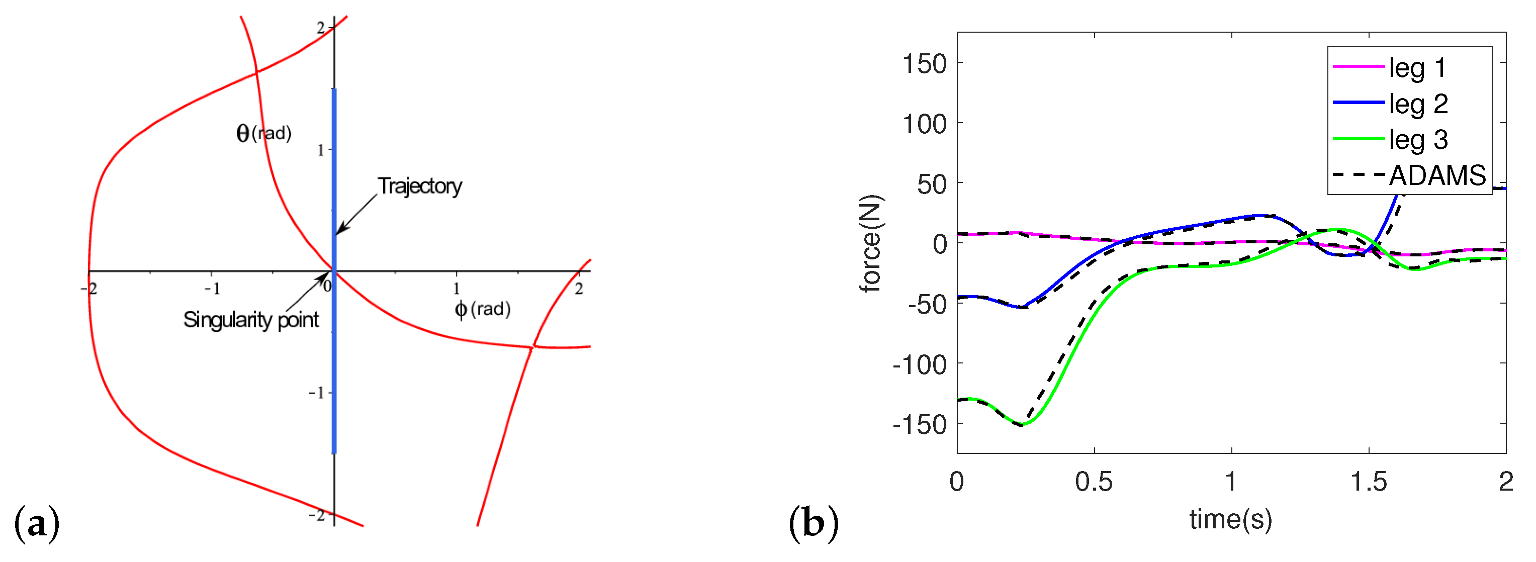
Let two architectures be defined, namely: $\alpha =\beta ={30}^{\circ }$ and $\alpha =\beta ={45}^{\circ }$. The moving platform is subjected to a 1-DOF motion characterized by the output variable $\theta$, and the other output variables are set to be $\varphi =\psi =0$. Jacobian A for each architecture can be computed and its zero sets are illustrated in the orientation workspace as shown in Figure 13 and Figure 14.

The motion path is generated in each architecture such that it passes through singularity at $\theta =0$. The moving platform following this path begins at $\theta =-{60}^{\circ }$ and terminates at $\theta ={60}^{\circ }$. All velocities, accelerations, and jerks at the beginning and end of the path are null. Let the whole path be completed in 1 s and the singularity occurs at $t=0.5$ s. The velocity, acceleration, and jerk at the singularity position are determined by fulfilling the first, second, and third conditions in Equations (14), (18) and (20). All those values become the boundary conditions for generating the 11th-degree polynomial trajectory, as follows:

$$\alpha =\beta ={30}^{\circ }\left\{\begin{array}{cccc}\theta \left(t_i\right)=-{60}^{\circ }\hfill & \dot{\theta }\left(t_i\right)=0\hfill & \ddot{\theta }\left(t_i\right)=0\hfill & \stackrel{⃛}{\theta }\left(t_i\right)=0\hfill \\ \theta \left(t_s\right)=0^{\circ }\hfill & \dot{\theta }\left(t_s\right)=2.64\hfill & \ddot{\theta }\left(t_s\right)=4.89\hfill & \stackrel{⃛}{\theta }\left(t_s\right)=-251.2\hfill \\ \theta \left(t_f\right)={60}^{\circ }\hfill & \dot{\theta }\left(t_f\right)=0\hfill & \ddot{\theta }\left(t_f\right)=0\hfill & \stackrel{⃛}{\theta }\left(t_f\right)=0\hfill \end{array}\right.$$

(28)

$$\alpha =\beta ={45}^{\circ }\left\{\begin{array}{cccc}\theta \left(t_i\right)=-{60}^{\circ }\hfill & \dot{\theta }\left(t_i\right)=0\hfill & \ddot{\theta }\left(t_i\right)=0\hfill & \stackrel{⃛}{\theta }\left(t_i\right)=0\hfill \\ \theta \left(t_s\right)=0^{\circ }\hfill & \dot{\theta }\left(t_s\right)=2.64\hfill & \ddot{\theta }\left(t_s\right)=4.51\hfill & \stackrel{⃛}{\theta }\left(t_s\right)=-192.2\hfill \\ \theta \left(t_f\right)={60}^{\circ }\hfill & \dot{\theta }\left(t_f\right)=0\hfill & \ddot{\theta }\left(t_f\right)=0\hfill & \stackrel{⃛}{\theta }\left(t_f\right)=0\hfill \end{array}\right.$$

(29)

and the trajectories are:

$$\begin{array}{cc}\theta {\left(t\right)}_{\alpha =\beta ={30}^{\circ }}=\hfill & -1.57+3450t^4-31100t^5+1.{22}^5{t}^6-2.67{10}^5{t}^7+3.51{10}^{5}t{}^8\hfill \\ \hfill & -2.72{10}^5{t}^9+1.16{10}^5{t}^{10}-21000t^{11}\hfill \end{array}$$

(30)

$$\begin{array}{cc}\theta {\left(t\right)}_{\alpha =\beta ={45}^{\circ }}=\hfill & -1.57+3120t^4-27800t^5+1.08{10}^5{t}^6-2.36{10}^5{t}^7+3.09{10}^5{t}^8\hfill \\ \hfill & -2.40{10}^5{t}^9+1.02{10}^5{t}^{10}-18500t^{11}\hfill \end{array}$$

(31)

The input forces when the moving platform tracing the 11th-degree trajectory are computed and the results are illustrated in Figure 15. The motor forces discontinuities at singularity can be discarded. The moving platform is now able to smoothly pass through singularity with finite input forces. The ADAMS simulation is performed to verify the approach as shown by the dashed line. The Mean Absolute Errors between the numerical results and the ADAMS simulation are 0.546, 1.073, and 1.657 for, respectively, the first, second and third leg.

5.3. Configuration III: $\alpha ={90}^{\circ }$

Configuration III performs a 3-DOF motion that belongs to the well-known 3-RPS parallel mechanism proposed by Hunt [41]. This motion is characterized by output variables $\mathbf{x}=\left[\begin{array}{ccc}\varphi & \theta & z\end{array}\right]$. It shows that the moving platform can perform pure translation along the z axis and two rotational motions, as written in Equation (32). This motion is driven by the input variables $\mathbf{q}=\left[\begin{array}{ccc}{q}_1& q_2& q_3\end{array}\right]$.

$${\mathbf{T}}_{\mathrm{III}}=\left[\begin{array}{cccc}-c_{\theta }(c_{\varphi }^2-1)+c_{\varphi }^2& (1-c_{\theta })s_{\varphi }{c}_{\varphi }& s_{\theta }{s}_{\varphi }& -b(c_{{\frac{\theta }{2}}^2}-1)(2c_{\varphi }^2-1)\\ (1-c_{\theta })s_{\varphi }{c}_{\varphi }& c_{\theta }{c}_{\varphi }^2+s_{\varphi }^2& -s_{\theta }{c}_{\varphi }& 2b(c_{{\frac{\theta }{2}}^2}-1)c_{\varphi }{s}_{\varphi }\\ -s_{\theta }{s}_{\varphi }& s_{\theta }{c}_{\varphi }& c_{\theta }& z\\ 0& 0& 0& 1\end{array}\right]$$

(32)

The direct-inverse Jacobians are determined by employing Equation (7) to the inverse kinematics equations g. The determinant of Jacobian A is computed, and a single equation in terms of Cartesian coordinates $(x,y,z)$ is found, as follows:

$$\begin{array}{cc}\mathcal{S}:\hfill & 38654705664x^{16}{y}^2+17179869184x^{16}{z}^2+206158430208x^{14}{y}^4+137438953472x^{14}\hfill \\ \hfill & y^2{z}^2+17179869184x^{14}{z}^4+429496729600x^{12}{y}^6+481036337152x^{12}{y}^4{z}^2-...=0\hfill \end{array}$$

(33)

Due to space limits, the polynomial equation $\mathcal{S}$ is written partially and its zero set is plotted in Cartesian space in Figure 16a.

Let the moving platform undergo a 1-DOF motion parametrized by a single parameter $\theta$ and the other output variables $(\varphi ,z)$ are assigned with specific values. Thus, the direct-inverse Jacobians of this motion are given, as follows:

$$\begin{array}{c}\varphi =0,z={\displaystyle \frac{3\sqrt{13}}{32}}\hfill \\ \mathbf{A}=\left[\begin{array}{ccc}-\frac{3}{2}\sqrt{13}{s}_{\theta }& -\frac{1}{2}{s}_{\theta }-\frac{1}{4}{s}_{2\theta }& 12\sqrt{3}\\ \frac{3}{4}\sqrt{13}{s}_{\theta }+\frac{3}{4}\sqrt{3}{c}_{2\theta }-6\sqrt{3}{c}_{\theta }+{\displaystyle \frac{21}{4}}\sqrt{3}& \frac{3}{4}\sqrt{39}{c}_{\theta }-\frac{1}{4}{s}_{2\theta }+4s_{\theta }& 8\sqrt{3}{s}_{\theta }+12\sqrt{13}\\ \frac{3}{4}\sqrt{13}{s}_{\theta }-\frac{3}{4}\sqrt{3}{c}_{2\theta }+6\sqrt{3}{c}_{\theta }+{\displaystyle \frac{21}{4}}\sqrt{3}& -\frac{3}{4}\sqrt{39}{c}_{\theta }-\frac{1}{4}{s}_{2\theta }+4s_{\theta }& -8\sqrt{3}{s}_{\theta }+12\sqrt{13}\end{array}\right]\hfill \\ \mathbf{B}=-128\left[\begin{array}{ccc}{q}_1& 0& 0\\ 0& q_2& 0\\ 0& 0& q_3\end{array}\right]\hfill \end{array}$$

(34)

The path of this motion crosses a point in the singularity surface in Figure 16 at $\theta ={60}^{\circ }$. The illustration of the motion path crossing the singularity curve is depicted in Figure 17a. Without respecting the first and second conditions, the motor forces will go unbound in the vicinity of singularity before $t=1$ s, as depicted in Figure 17a. Likewise, the simulation results by ADAMS stop before the singularity because the needs of motor torques leading up to singularity are too high and too sudden. The ADAMS simulation depict it as discontinued forces even before 1 s.

For the mechanism to be able to pass through the singularity, the first, second, and third conditions should be fulfilled. Hence, the boundary conditions are as follows:

$$\begin{array}{cccc}\theta \left(t_i\right)={30}^{\circ }\hfill & \dot{\theta }\left(t_i\right)=0\hfill & \ddot{\theta }\left(t_i\right)=0\hfill & \stackrel{⃛}{\theta }\left(t_i\right)=0\hfill \\ \theta \left(t_s\right)={60}^{\circ }\hfill & \dot{\theta }\left(t_s\right)=1.42\hfill & \ddot{\theta }\left(t_s\right)=0.67\hfill & \stackrel{⃛}{\theta }\left(t_s\right)=9.1\hfill \\ \theta \left(t_f\right)={90}^{\circ }\hfill & \dot{\theta }\left(t_f\right)=0\hfill & \ddot{\theta }\left(t_f\right)=0\hfill & \stackrel{⃛}{\theta }\left(t_f\right)=0\hfill \end{array}$$

(35)

By taking into account these boundary conditions, the 11th-degree polynomial trajectory is generated, as follows:

$$\theta \left(t\right)=0.524-57.3t^4+290t^5-616t^6+703t^7-477t^8+190t^9-41.2t^{10}+3.79t^{11}$$

(36)

The results of numerical simulation with the 11th-degree polynomial trajectory written in Equation (36) are plotted in Figure 17b. It shows that the input forces are finite and there are no discontinuities when passing through the singularity at $t=1$ s. These results have been confirmed by the ADAMS simulation as shown by the dashed lines. The Mean Absolute Errors between the numerical results and the ADAMS simulation are 0.106, 0.381, and 0.373 for, respectively, the first, second and third leg.

6. Conclusions

In the neighborhood of and at singularities, the dynamic behaviors of parallel mechanisms become uncontrollable. This paper discusses unified solutions of dynamic models of a 3-(rR)PS metamorphic parallel mechanism to cross singularities. The inverse kinematics were derived with respect to time to determine the direct-inverse Jacobians, which are useful for describing the dynamic model based on Lagrange energy formulation. The input forces of all three configurations grew unbounded at the singularity. To solve this problem, the first, second, and third conditions that consist of the consistency condition, and the first and second indeterminate forms, were described. Compared to previous works [33,34,38], all three conditions ensure that any configuration can pass through singularity with a finite effort, which eventually introduces a jerk to the system. The jerk also becomes the boundary condition for generating the 11th-degree polynomial trajectory. This trajectory is plotted together with the singularity curves/surfaces of each configuration to better visualize the circumstances. The results show that Configurations I, II, and III can pass through singularities with finite input forces. The ADAMS simulation has confirmed the computational results.