1. Introduction
The problem of energy and the environment is becoming a growing concern in many countries [
1]; therefore, low-emission and high-efficiency power plants are urgently needed [
2]. With the advantages of low carbon emission and efficient energy utilization, the gas turbine is a new generation of power plant [
3,
4]. Because of these advantages, gas turbines have been widely used in aircraft power, land power generation, and marine power in recent years. The power output demand of ship power is increasing [
5]. In terms of operation performance, marine gas engines have a smaller unit power weight than steam and diesel engines and, thus, have better starting and acceleration performance and obvious advantages, such as low vibration and noise during operation [
6,
7].
Benefiting from the increasingly mature aero-engine technology, marine gas turbines based on aero-engines have been widely used. Marine gas turbines can significantly improve the dynamic performance of ships and have gradually become the main power device of the surface warships of various countries and one of the important symbols of naval equipment modernization [
8]. Marine gas turbines have gradually been developed toward high power, high efficiency, and low emissions [
9,
10].
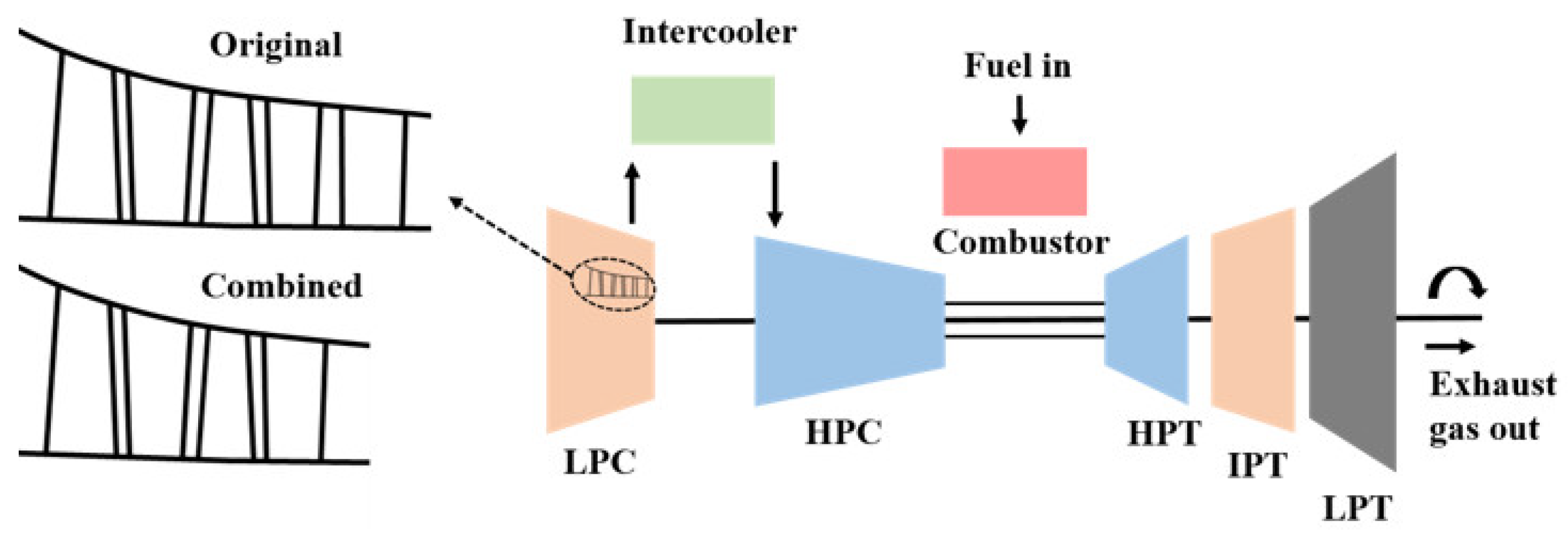
In recent years, the demand for large ships has increased, implying increased engine performance requirements. The performance of marine gas turbines can be improved in two ways: (1) the performance can be improved by increasing the pressure ratio, the turbine inlet temperature, and the component efficiency without changing the original cycle structure; and (2) complicated cycles, such as intercooling, can be adopted to improve the gas turbine performance [
11]. In the intercooling cycle, the fluid is initially compressed in a low-pressure compressor and flows into the intercooler for cooling. After cooling, the fluid is sent to the entrance of a high-pressure compressor where the fluid is further compressed [
12]. Intercooling technology can effectively reduce the power consumption of compressors [
13,
14]. For high-power marine gas turbines, a complex cycle gas turbine that adopts a mature core engine and increases power through intercooling is preferred [
9].
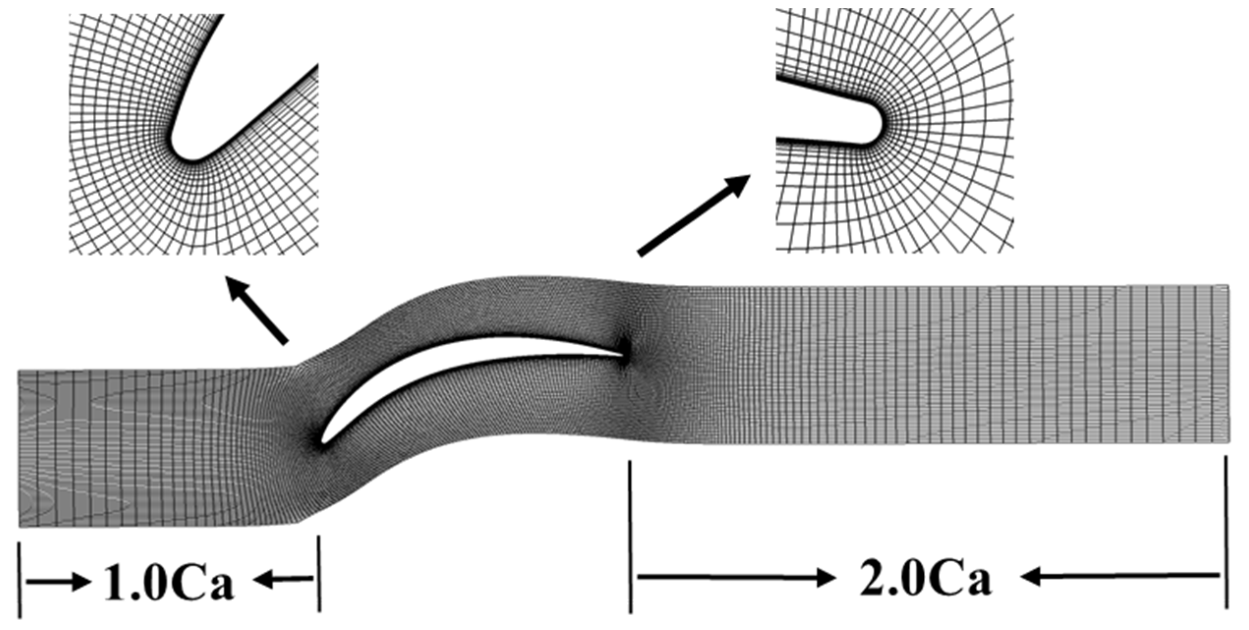
Limited by space, marine gas turbines should be small and have a compact structure. To improve the gas turbine performance, a simple cycle can be changed into an intercooling cycle. In the refit process, an intercooler, air duct, outlet guide vane, and other structures must be installed, complicating the structure and increasing the space size. To improve this situation, a last-stage stator and an outlet guide vane of the low-pressure compressor can be combined, allowing a single large turning blade to simultaneously compress air and guide flow, as shown in
Figure 1. The use of this blade can reduce the number of compressor blades, effectively simplify the structure of the intercooling cycle, and reduce the size and weight of marine gas turbines.
Sahu et al. [
15] carried out a thermo-economic analysis of the intercooling cycle and obtained the cost of gas turbine cycles. Kumari et al. [
16] studied the effect of the intercooling cycle on emission performance and found that the intercooling cycle can reduce CO and NOx emissions to a certain extent. Li et al. [
17] established a simulation model of a marine intercooled gas turbine and studied the optimal oil supply law of the intercooled gas turbine during acceleration. Zhang and Hassene [
18,
19] carried out numerical simulations and experimental measurements of the intercooler, and explored the effect of temperature, flow rate, and geometric size. Wang [
20] conducted the aerodynamic design and flow-field analysis of the low-pressure compressor of the intercooled cycle gas turbine. Scholars have studied the intercooling cycle from different aspects, but there is a lack of relevant analysis on the combination of the last-stage stator and outlet guide vane into a single blade to reduce the weight and size of the compressor.
The analysis of the blade can be started from the profile. As the most basic unit to establish the diffusion flow field of the compressor, the profile of the compressor plays an extremely important role in the overall performance of the compressor. In the development of the blade’s aerodynamic profile, many scholars have conducted much research on it. The National Advisory Committee for Aeronautics (NACA) [
21] conducted cascade aerodynamic experiments on a large number of profiles with good subsonic performance, namely, NACA 65 profiles. After that, NACA [
22] found that by reducing the maximum thickness of the leading edge, double arc airfoils (DCA) with better supersonic performance could be obtained. Elazar et al. [
23] found that the loss near the design condition and the low loss range of controlled diffusion airfoils (CDA) are better than that of DCA. Due to the two-dimensional design method of the original CDA, the three-dimensional flow was not considered. Behlke [
24] proposed the design idea of the second-generation controlled diffusion airfoils (CDA-II), which can improve the efficiency by 1.5% and surge margin by 8%. Song and Gu [
25] realized the CDA design with continuous leading-edge curvature and eliminated the leading-edge velocity spikes. Most researches on compressor profile focus on enhancing the diffusion capacity and reducing the flow loss, but there is a lack of corresponding research on the large turning profile which increases the flow turning capacity.
A new idea is proposed to combine the two rows of blades of the last-stage stator and the outlet guide vane of the compressor into a single row of blades so as to reduce the weight and size of the compressor, which is especially suitable for the intercooling cycle marine gas turbine with strict weight and size requirements. One of the key problems brought by this idea is that the profile has a large turning angle, up to 60–70 degrees. At present, there are few studies on similar profiles and it is urgent to verify the feasibility of this type of compressor profile with a large turning angle. In this paper, which aims at the large turning profile designed by combining the last-stage stator and the outlet guide vane of the low-pressure compressor of an intercooling cycle marine gas turbine, the macroscopic characteristics, flow characteristics, load characteristics, and loss characteristics are analyzed by means of experiment and numerical simulation. The feasibility of this profile as a combined profile is studied, providing a reference for the aerodynamic and structural design of marine gas turbines.
2. Plane Cascade Experiment
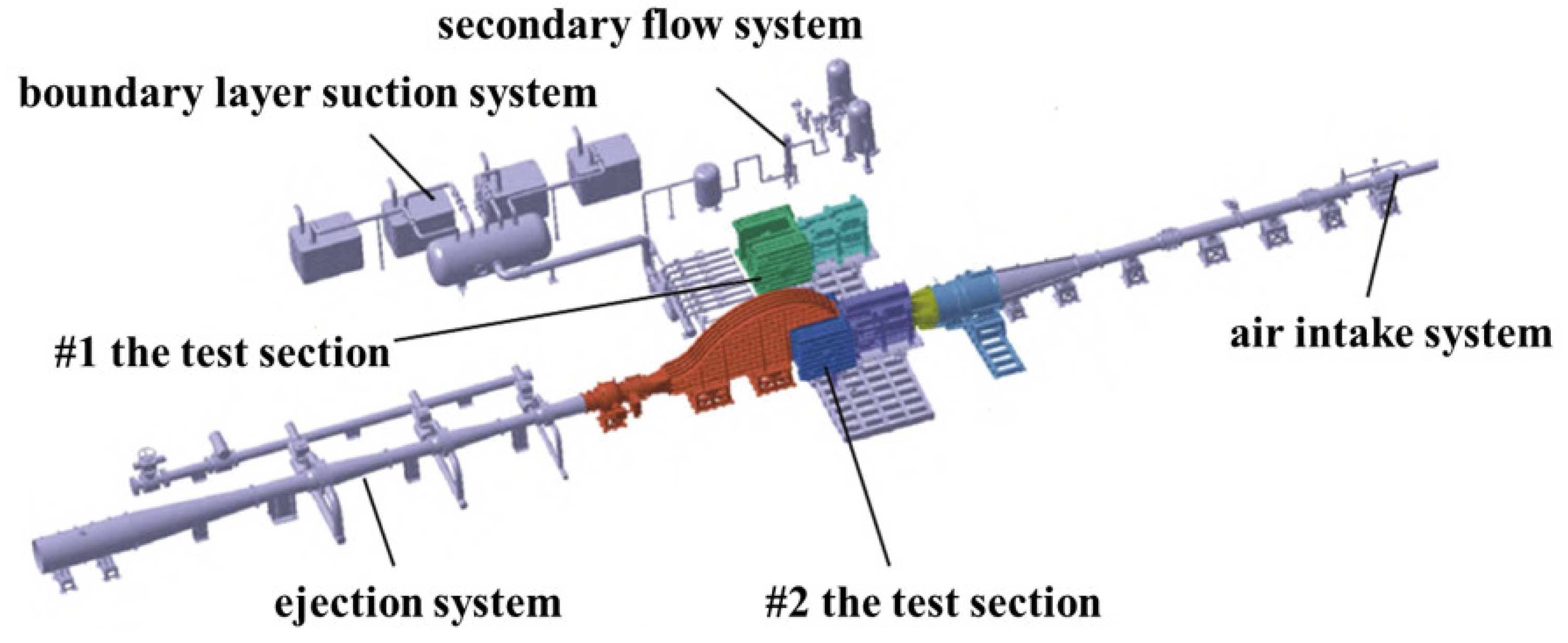
In order to study the feasibility of combining the last-stage stator and outlet guide vane into a single profile from the perspective of aerodynamic performance, the combined profile was stretched into a straight cascade and the aerodynamic parameters of the cascade were measured through the plane cascade blowing test. The test was carried out in a variable density plane cascade wind tunnel, which is composed of the air intake system, the test section, the ejection system, the secondary flow system, the boundary layer suction system, and the measurement and control system, as shown in
Figure 2 [
26]. In the test, air was supplied by a medium-pressure air source. Air entered the medium-pressure gas-storage tank after purification and drying and then directly supplied to the equipment through the pipeline [
27].
The total temperature, the total pressure, the wall static pressure, and the flow angle were measured in the plane cascade experiment. The total parameters at the inlet of the test section were measured in the stable section of the wind tunnel. The total temperature was measured by two T-type thermocouples, with a maximum temperature precision of 0.55 °C in the temperature range of −40–120 °C. The total pressure was measured by two PPT pressure sensors, with a sensor-verification accuracy of 0.02%. The mean value of the total temperature and pressure at the inlet was obtained through average length measurement. The pressure parameters of the wind tunnel were measured by an electronic pressure-scanning valve, with a measurement error of less than 0.05%. The wake parameters of the cascade were measured by a calibrated porous pneumatic probe. A microcomputer-controlled stepper motor drove the probe to move and measure the pressure at discrete points along the cascade distance. The moving precision of the probe can reach 0.1 mm.
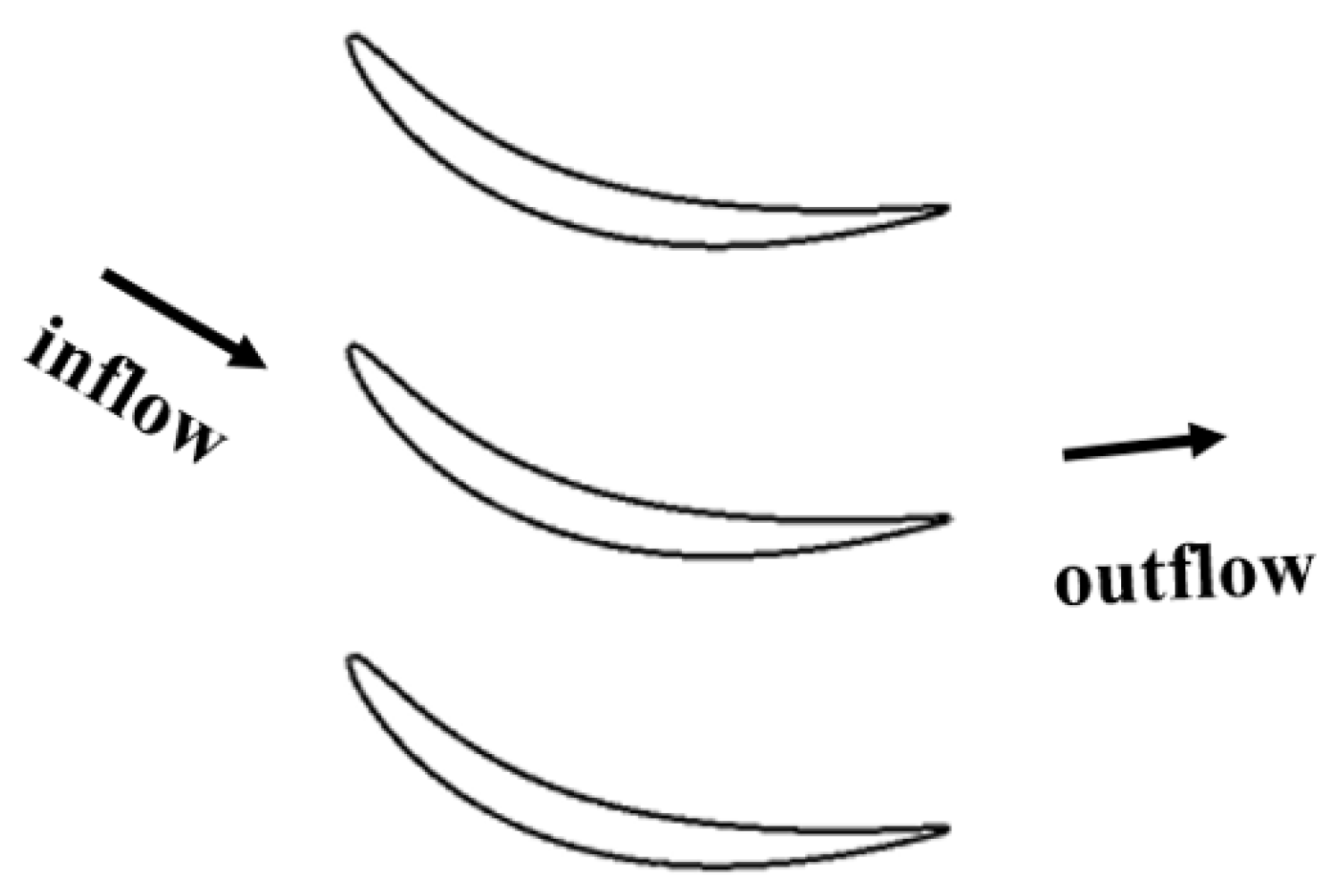
The experimental model is a three-dimensional straight cascade channel, and its cross-section is shown in
Figure 3. The cross-section of the blade shows that the geometric turning angle of the profile is 67°, which has a large turning property. The parameters of the three-dimensional straight cascade channel are summarized in
Table 1.
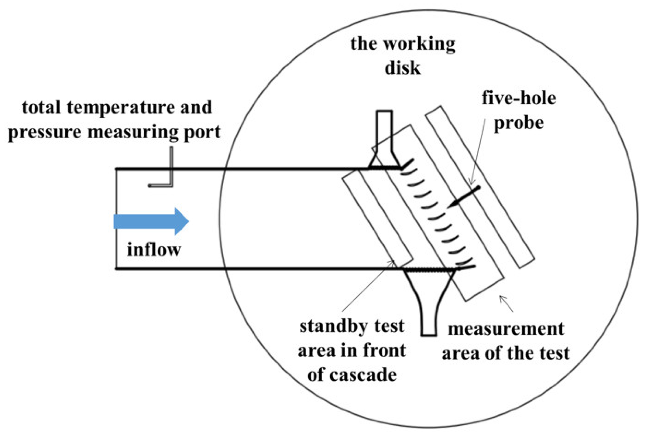
Figure 4 is a schematic of the test section of the experiment, which is mainly composed of the left and right wall surfaces, a disk, and the upper and lower wall panels. The experimental model is mounted on the disk. The experiment aims to study the change of the inlet and outlet parameters and the pressure distribution of the cascade when the angle of attack changes. For the measurement on the cascade, a set of parameters were measured along the circumference of a small distance, and then the average value of the measured parameters of many measuring points within a blade distance was taken. After measuring the relevant data of an angle of attack, the angle of attack was changed by manually turning the working disk of the test section. The airflow angle could be adjusted from 20° to 160°.
4. Performance Analysis
To compare and analyze the aerodynamic performance of the profile under different Mach numbers and angles of attack and explore the rationality of the blade profile as a low-pressure compressor-outlet profile, the results at 50% blade height were analyzed mainly from four aspects: macroscopic characteristics, flow characteristics, load characteristics, and loss characteristics.
4.1. Macroscopic Characteristics
Figure 7 shows the characteristic curves of the total pressure loss with the angle of attack at different Mach numbers. The total pressure-loss coefficients with Mach numbers of 0.2 and 0.4 at different angles of attack were obtained by the experimental and numerical methods, respectively. The numerical results are consistent with the experimental results.
The low-loss operating range is the angle-of-attack range where the total pressure-loss coefficient is less than or equal to twice the total pressure-loss coefficient of the lowest loss point. According to the test results, when the inlet Mach number was 0.2, the choke point was −12.76°, the stall point was +3.55°, and the low-loss operating range was 16.31°; when the inlet Mach number was 0.4, the choke point was −10.59°, the stall point was +1.98°, and the low-loss operating range was 12.57°. The working range of the numerical results is similar to that of the test. With the increase in the inlet Mach number, the total pressure loss of the blade profile decreased at a small angle of attack, and the low-loss operating range decreased. Although the total pressure loss surges due to the change in flow state when the angle of positive attack increases to a certain range, this blade profile still has the characteristics of low overall loss and wide range of working conditions.
4.2. Flow Characteristics
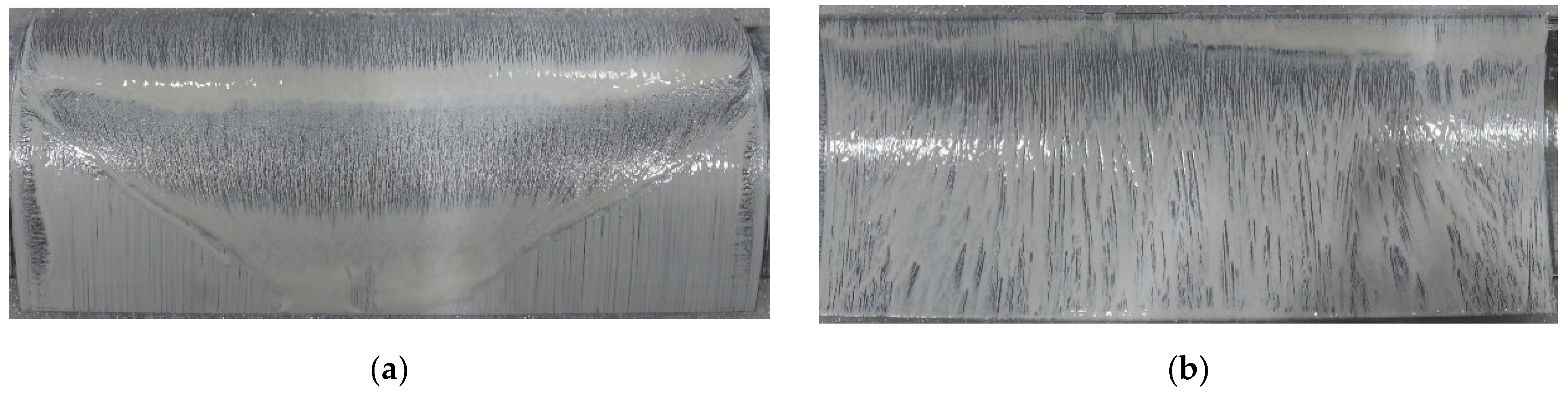
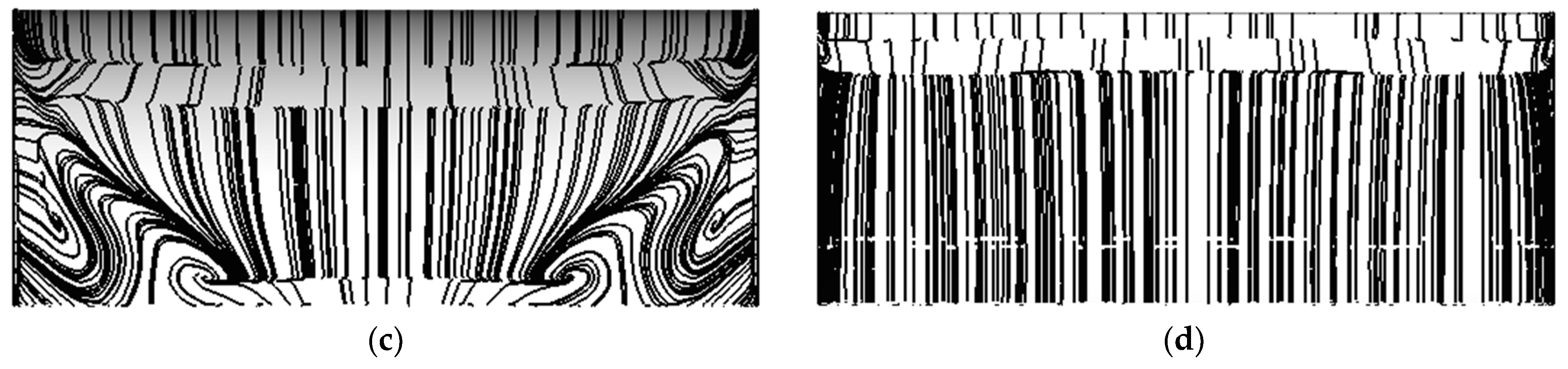
Taking the cascade as the test object, the oil flow test was carried out at the inlet Mach number of 0.2. When the inlet angle of attack was −3°, separation bubbles existed on both the suction and pressure surfaces in the front part of the blade, and the flow situation was near the numerical results, as shown in
Figure 8.
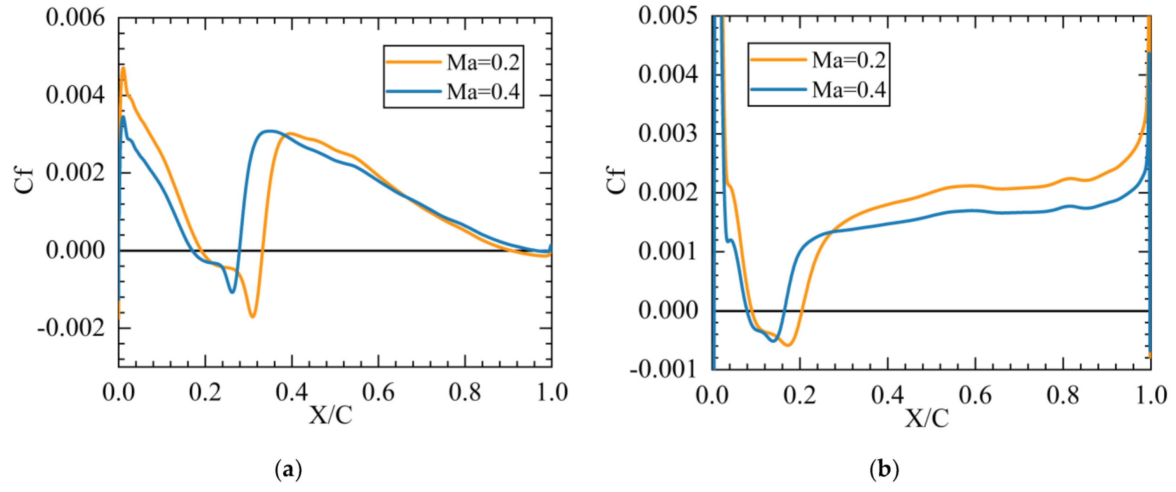
Figure 9 shows the skin-friction coefficient distribution. As the inlet Mach number increased from 0.2 to 0.4, the separation strength decreased. For the suction surface, the separation position moved from 19.1%C to 17.0%C, and the attachment position moved from 33.2%C to 27.9%C. The separation bubble size changed from 14.1%C to 10.9%C. For the pressure surface, the separation position moved from 8.9%C to 7.9%C, the attachment position moved from 20.5%C to 16.5%C, and the separation bubble length changed from 11.6%C to 8.6%C. The change in flow state caused by the change of the separation bubble is closely related to the decrease in the total pressure loss.
Figure 10 shows the shape factor distribution under different Mach numbers. The shape factor is expressed as δ1/δ2, where δ1 represents the displacement thickness of the boundary layer, and δ2 represents the momentum thickness of the boundary layer [
29]. The shape factor distribution of the suction and pressure surfaces is similar. Initially, the flow is laminar flow, and the shape factor increases from approximately 2.0 near the stagnation point to approximately 5.0 at the separation point. Then, the shape factor drops to less than 2.5, and the flow becomes turbulent. The comparison of the shape factors of different Mach numbers reveals that after the Mach number increases from 0.2 to 0.4, the peak of the shape factor characterizing the separation bubble moves forward. After the transition to turbulent flow, the shape factor of Mach number 0.4 is always lower than that of Mach number 0.2.
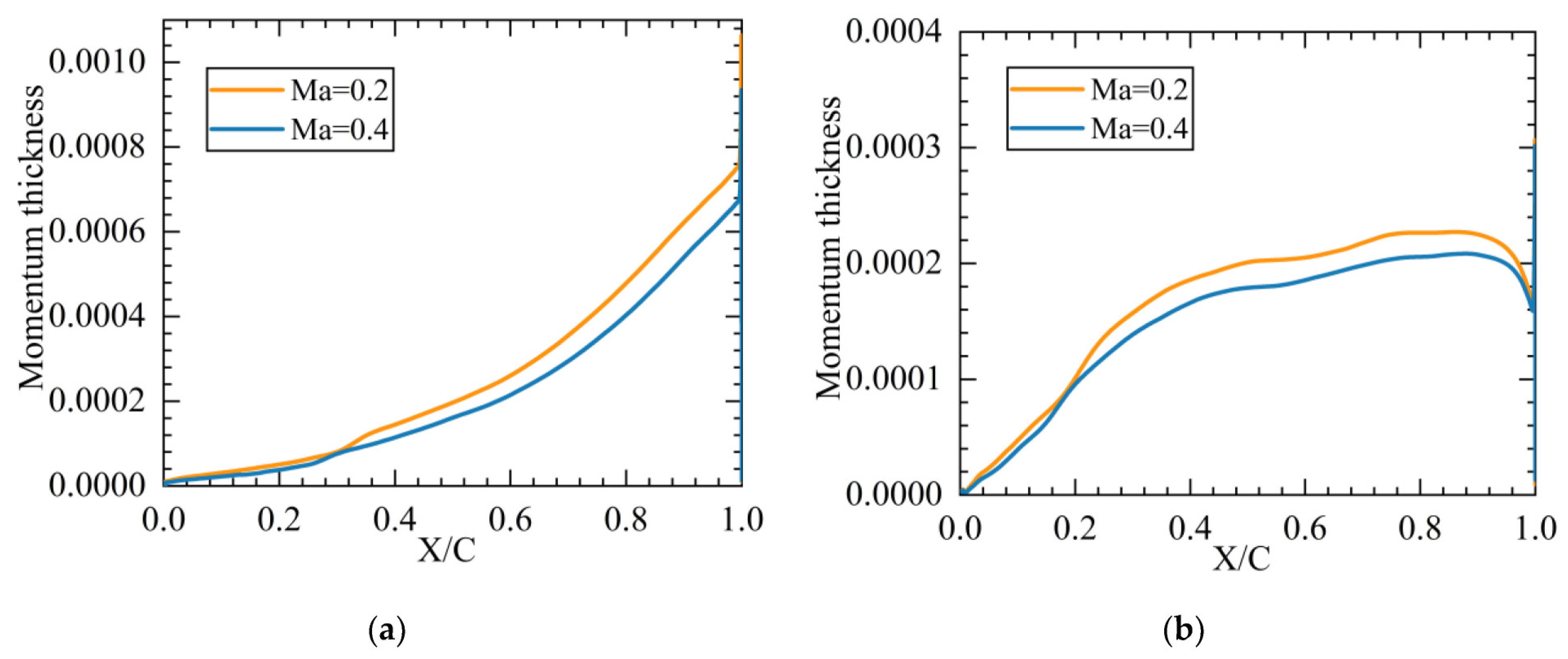
As shown in
Figure 11, the momentum thickness of both the suction and pressure surfaces decreases with the increase in the Mach number. The loss related to the boundary layer decreases with the momentum thickness, resulting in the decrease in the total pressure loss. Along the flow direction, the momentum thickness of the suction surface increases gradually, while the momentum thickness of the pressure surface increases first and then decreases.
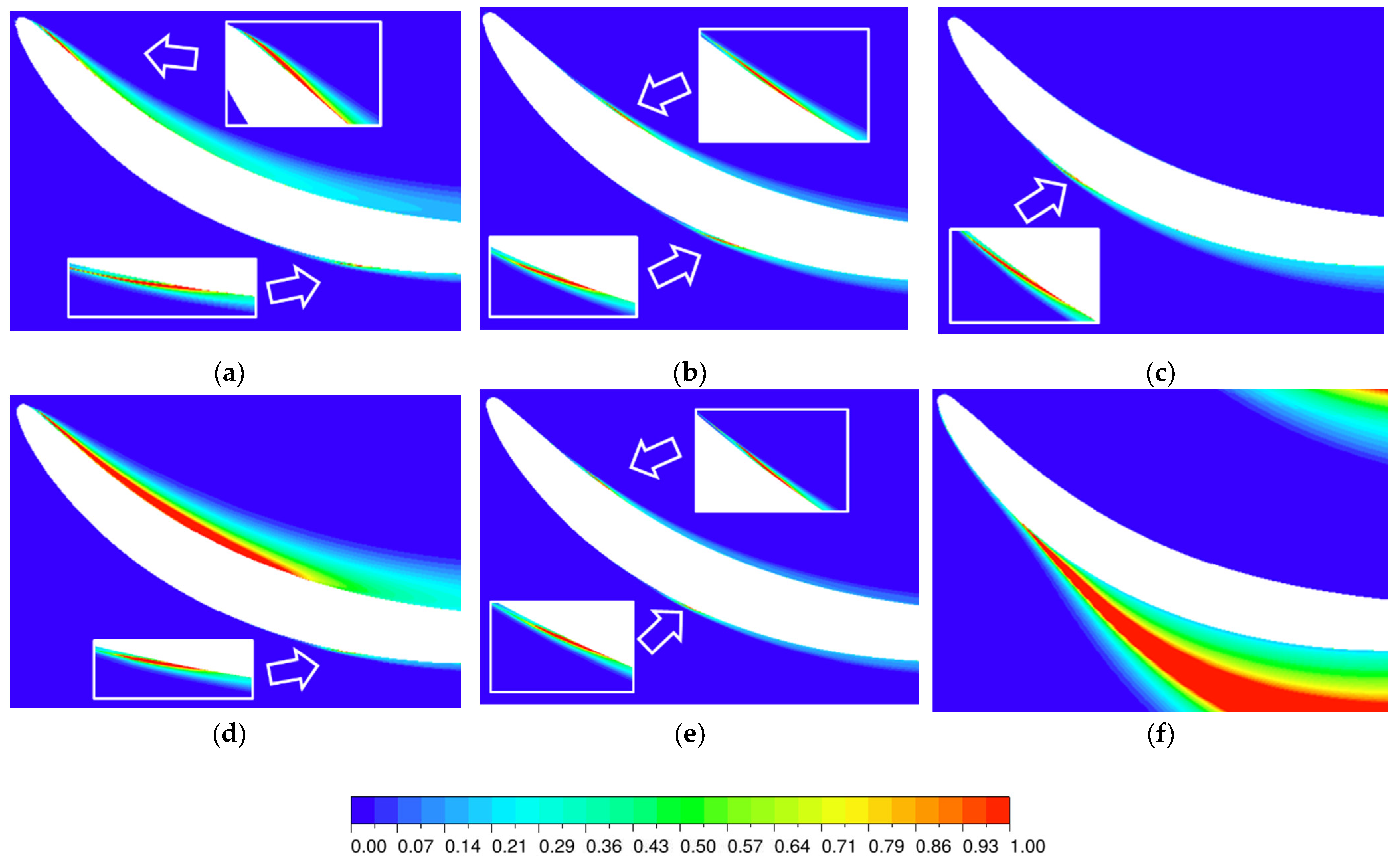
Figure 12 shows the contour of the turbulence intensity at different angles of attack when the inlet Mach number is 0.2 and 0.4. When the angle of attack is −12° and the inlet Mach number is 0.2, the pressure surface near the leading edge and the suction surface near the middle have a high turbulence intensity, indicating the existence of flow separation [
25]. When the Mach number increases to 0.4, a small separation bubble remains on the suction surface, and the size of the separation bubble on the pressure surface increases. When the angle of attack is −3°, the separation position of the pressure surface is nearer the leading edge than that of the suction surface. When the angle of attack is +4°, for the pressure surface, the flow does not separate when the inlet Mach number is 0.2 and 0.4. The analysis of the turbulence intensity near the suction surface shows that when the inlet Mach number is 0.2, only a small separation bubble exists in the front part of the blade; however, when the inlet Mach number is 0.4, after flow separation occurs on the suction surface, the fluid fails to attach to the wall again and open separation occurs. Further analysis reveals that when the inlet Mach number is 0.2 and the angle of attack increases to +5°, a large separation of the suction surface will also occur. The large-scale separation near the suction surface leads to a sharp increase in the separation loss, resulting in a sudden increase in the total pressure-loss coefficient at the angle of positive attack; however, this sudden increase in the loss only occurs at the large angle of positive attack. At the small angle of positive attack, separation still occurs in the form of a separation bubble, and the total pressure loss is low.
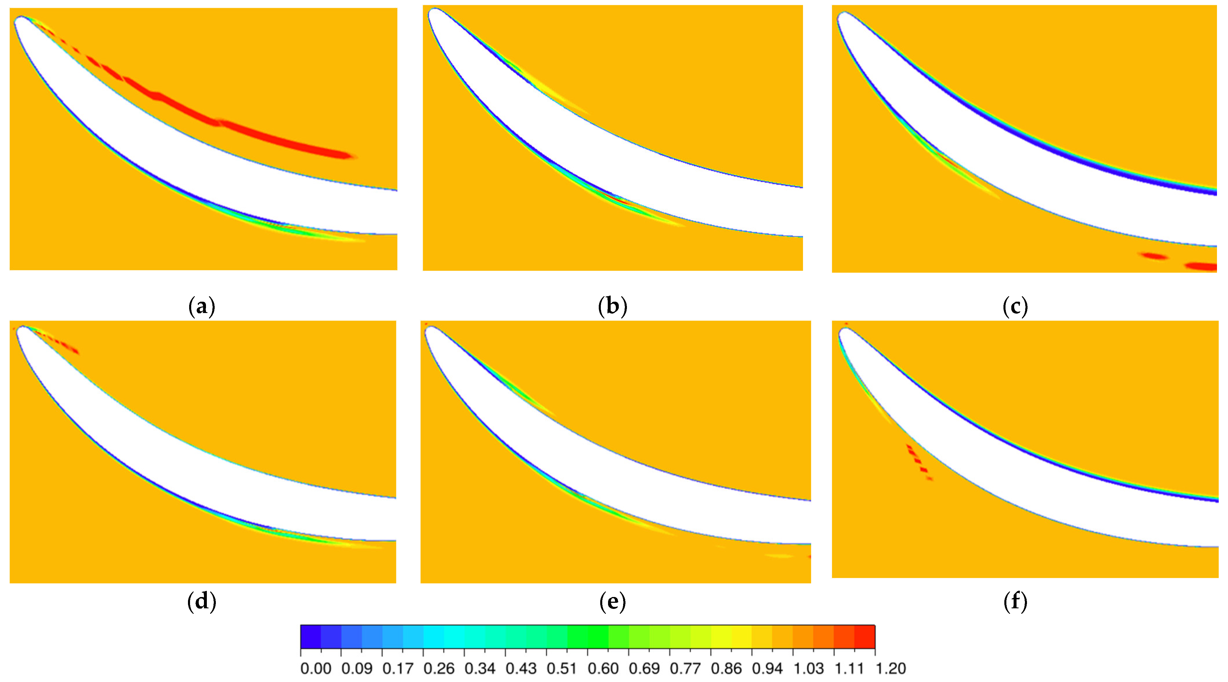
The flow transition under different working conditions can be effectively understood through the intermittent factor, as shown in
Figure 13. The intermittent factor is 0 when the flow is completely laminar, the flow state between 0 and 1 is transition state, and the flow state is 1 when the flow is completely turbulent [
30]. When the inlet angle of attack is −12° and −3°, the intermittency factors of Mach numbers 0.2 and 0.4 increase sharply near the front half of the pressure surface and the middle of the suction surface, indicating that transition occurs at these positions. When the inlet angle of attack is +4°, the intermittent factor is always near 0 at the pressure surface, so the flow at the pressure surface is laminar at both Mach numbers. For the suction surface, when the Mach number is 0.2, transition occurs at the first half of the blade; when the Mach number is 0.4, the wide range of open separation has a great separation strength, causing transition soon after the flow begins to separate. Combined with the previous flow analysis, the analysis of the flow transition shows that at this time, flow separation exists near the transition, and the transition form is mostly separation bubble transition.
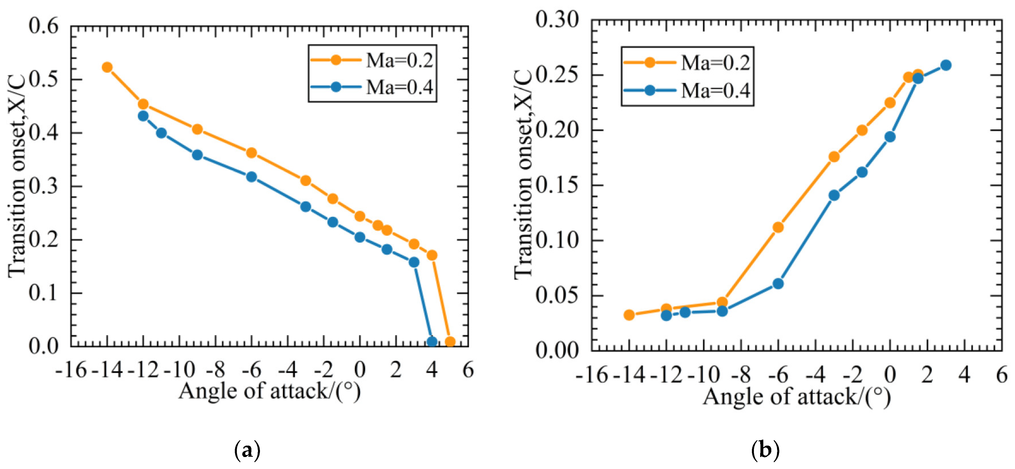
Figure 14 summarizes the changes in transition positions at different angles of attack. As the angle of attack moves from the negative angle of attack to the positive angle of attack, the transition position on the suction surface gradually moves from the middle position of the profile to the leading edge. The relationship between the transition position and the angle of attack is linear as a whole; however, when the angle of attack increases to approximately +4°, the transition position suddenly moves forward, the flow suddenly becomes a wide range of open separation, and the total pressure loss sharply increases. For the pressure surface, the transition position moves backward from near the leading edge to approximately 25% of the chord length of the profile as the angle of attack moves toward the positive angle of attack. If the angle of attack moves further toward the positive angle of attack, transition no longer occurs, and the flow state near the pressure surface is laminar. The analysis of the specific separation indicates that the transition position is related to the location of separation, that is, the existence of separation will induce separation bubble transition and is related to the separation intensity, that is, the high intensity of separation results in the immediate transition of the flow after the separation.
4.3. Load Characteristics
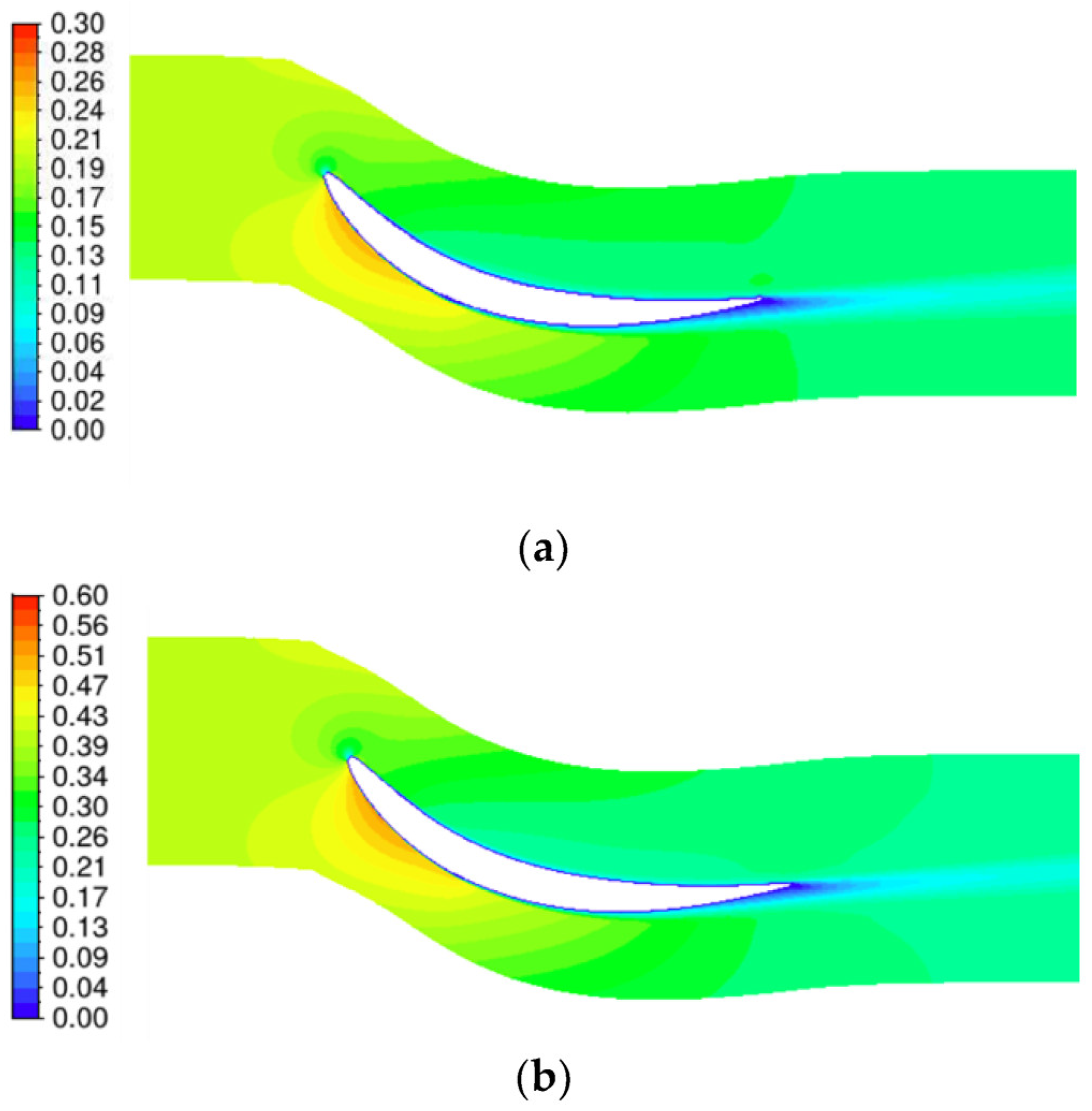
Figure 15 shows the Mach number distribution at inlet Mach numbers 0.2 and 0.4. When the inlet Mach number is 0.2 and 0.4, the load distribution is similar, and the maximum Mach number is concentrated near the leading edge. When the inlet Mach number is 0.2, the peak Mach number is 0.254, and when the inlet Mach number is 0.4, the peak Mach number is 0.518. In the experiment, the static pressure distribution on the surface of the blade was measured by pressure measuring holes.
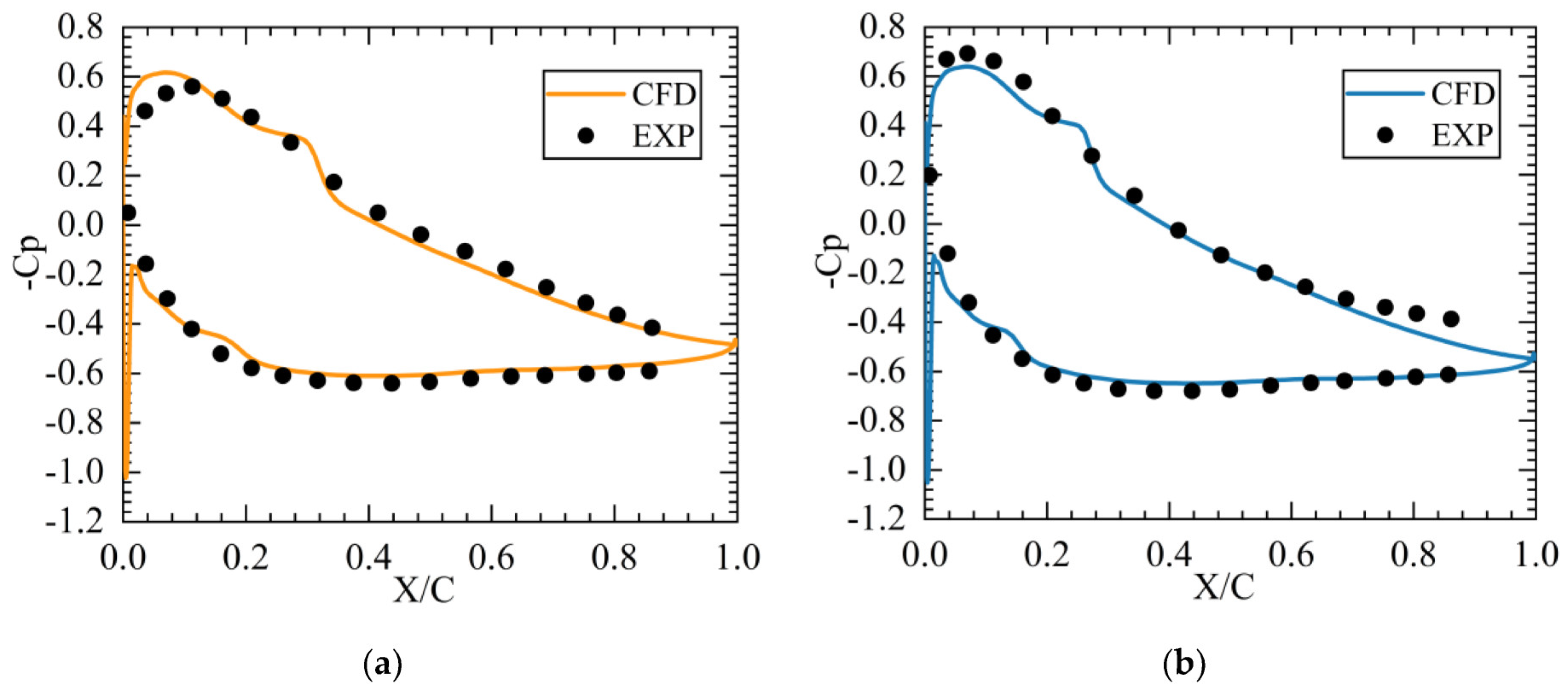
Figure 16 shows the static pressure coefficient distribution at the angle of attack of −3° when the inlet Mach number is 0.2 and 0.4. The static pressure coefficient distribution calculated by numerical method is consistent with that of the experiment. Near the leading edge, the load distributions of the two Mach numbers are not much different. Given that the separation bubble moves forward when the Mach number is 0.4, the load distribution after the separation bubble is different, that is, the load when the inlet Mach number is 0.2 is less than that when the inlet Mach number is 0.4.
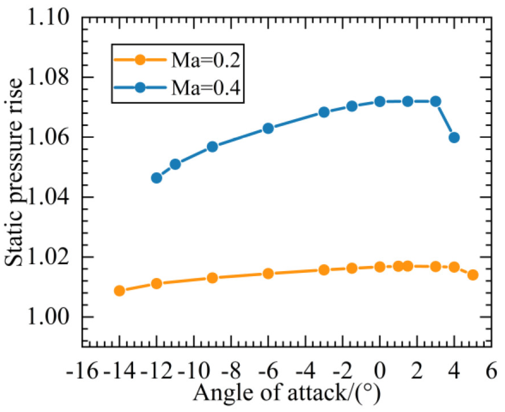
The load performance in the entire working condition can be analyzed in
Figure 17 and
Figure 18. In
Figure 17, the static pressure rise increases first and then decreases as the angle of attack moves from negative to positive. When the positive angle of attack increases to a certain extent, the open separation on the suction surface changes the diffusion capability, and the static pressure rise decreases.
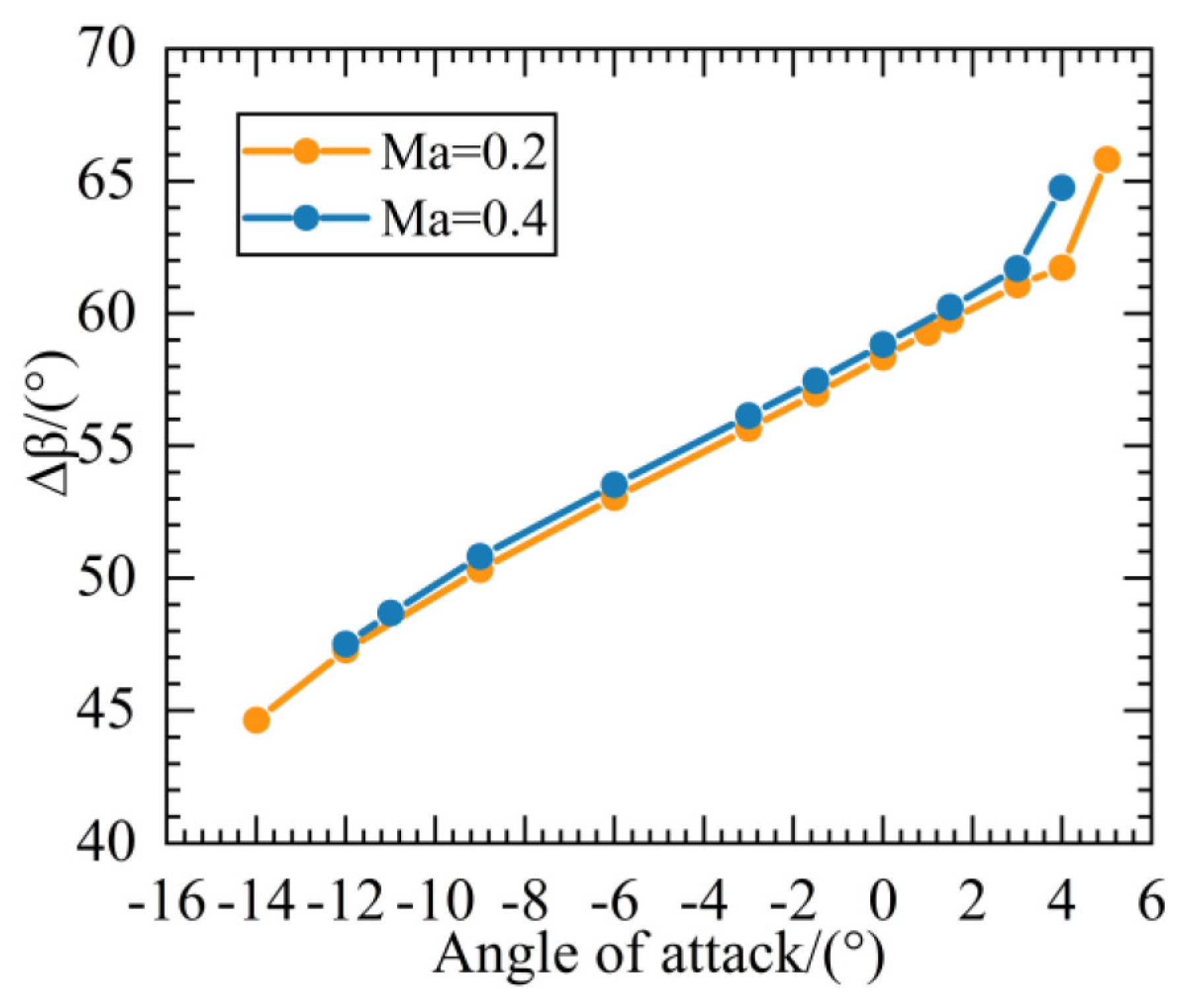
Figure 18 shows that as the angle of attack moves from the negative angle of attack to the positive angle of attack, the flow turning angle increases and is approximately linearly distributed. When the positive angle of attack increases to a certain extent, a large range of separation appears near the suction surface, making the air flow deviate toward the pressure surface near the trailing edge. At this time, the outlet flow angle increases, resulting in the increase in the flow turning angle. Generally, a large flow turning angle exists at both Mach numbers, and the profile has a large turning property.
4.4. Loss Characteristics
To specifically analyze the loss characteristics of the profile, different loss calculation methods were combined to analyze the local and global losses.
Traditional loss analysis shows a cumulative effect. The dissipation function can directly represent the specific source and increasing process of the local loss in the flow channel, providing a perfect method for loss analysis [
31].
First, the dissipation function is derived using the energy equation in entropy form:
is the viscous dissipation of the laminar flow, and is dissipation caused by the turbulent Reynolds stress. The viscous stress tensor is obtained through the time average. The turbulence model is the eddy–viscosity model (EVM). The Boussinesq eddy–viscosity hypothesis is used to calculate the Reynolds stress. Two types of dissipation are calculated as follows.
The viscous stress tensor is:
The time average of this tensor is written as:
The laminar dissipation is:
In the three-dimensional case, it can generally be written as:
The turbulent dissipation is:
The dissipation coefficient is obtained with the non-dimensional processing of the dissipation function. The formula of the dissipation factor obtained is shown in the following equation:
is the chord length of the profile. and are the density and the inlet velocity, respectively.
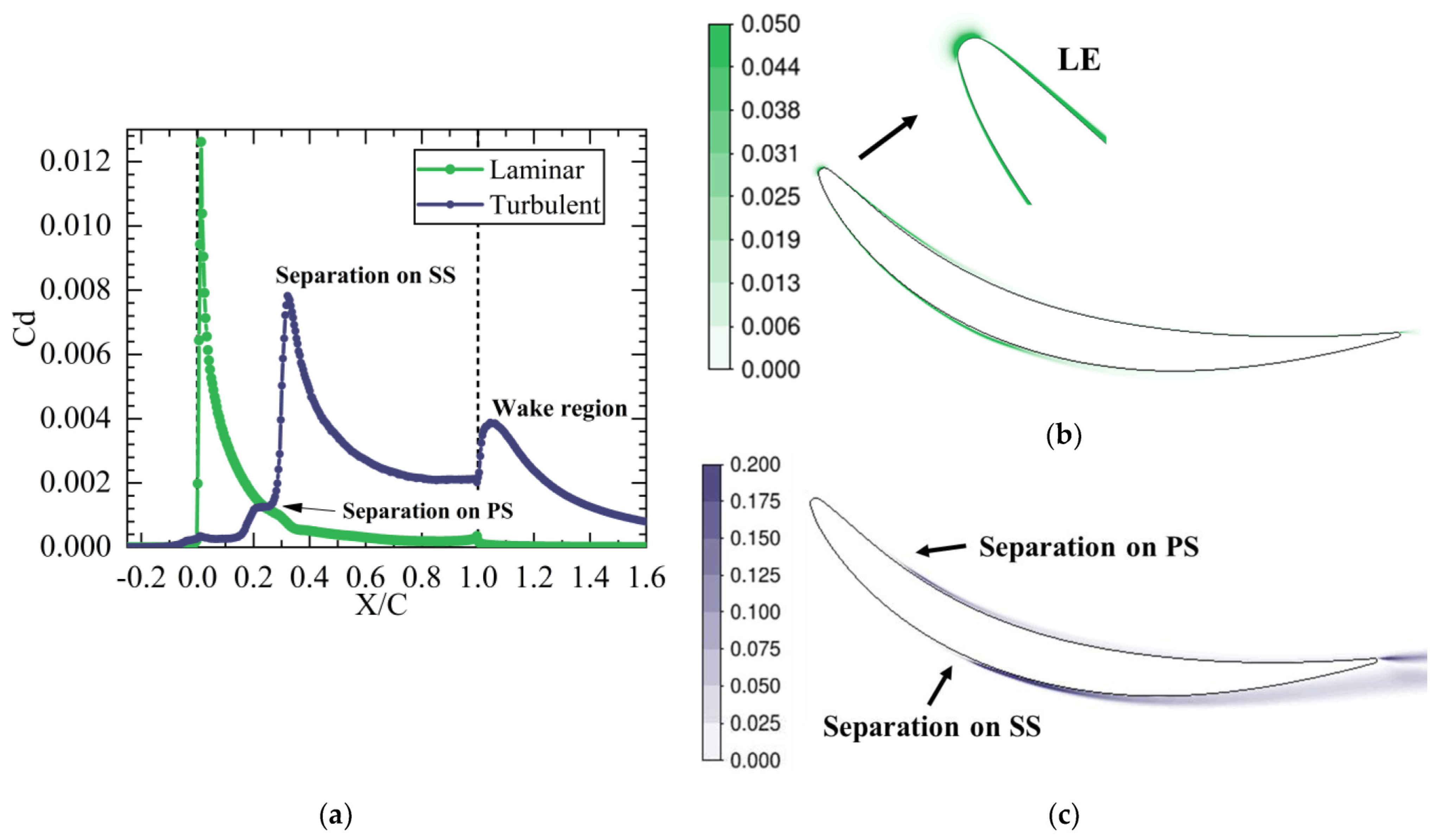
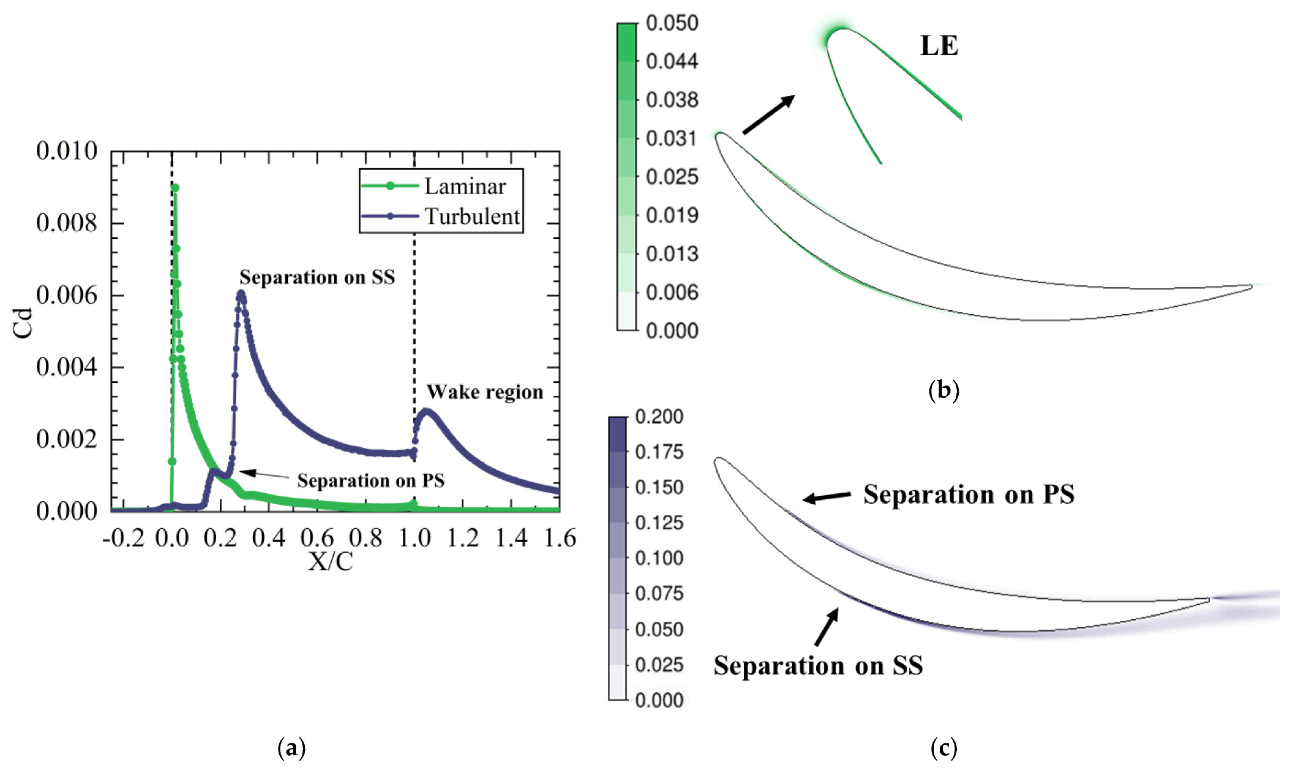
The source of the main loss can be obtained by analyzing the high dissipation area and the flow phenomenon in the flow field. As shown in
Figure 19 and
Figure 20, the laminar and turbulent dissipations can be analyzed separately to distinguish and compare the losses caused by laminar and turbulent flows. The position where X/C = 0 is the leading edge of the profile, and the position where X/C = 1 is the trailing edge of the profile. The comparison of the dissipation distribution between different Mach numbers reveals that when the angle of attack is −3°, the dissipation distribution with Mach numbers of 0.2 and 0.4 is similar. Laminar flow dissipation is the main dissipation in the first half of the blade profile. When transition occurs on the suction and pressure surfaces, laminar dissipation decreases gradually, and turbulence dissipation becomes the main dissipation.
According to the dissipation distribution, laminar flow dissipation reaches its maximum value near the leading edge of the profile and mainly exists near the boundary layer of the profile, which is mainly caused by the shear force in the boundary layer. The turbulent dissipation is nearly 0 at the beginning. With the appearance of separation bubble transition on the pressure surface near the 20% chord length, the separation loss increases, and the turbulent dissipation reaches a small peak. The transition of the separation bubble occurs on the suction surface near the 30% chord length, and the superposition of turbulent losses on the suction and pressure surfaces causes the turbulent dissipation to reach a peak. When the air flows from the suction and pressure surfaces to the trailing edge of the profile, the boundary layers on both sides converge and become the wake of the profile. In the wake region, the vortex region is generated. Owing to the viscous effect, the kinetic energy consumed in these processes is converted into heat energy, which increases the turbulent dissipation in the wake region.
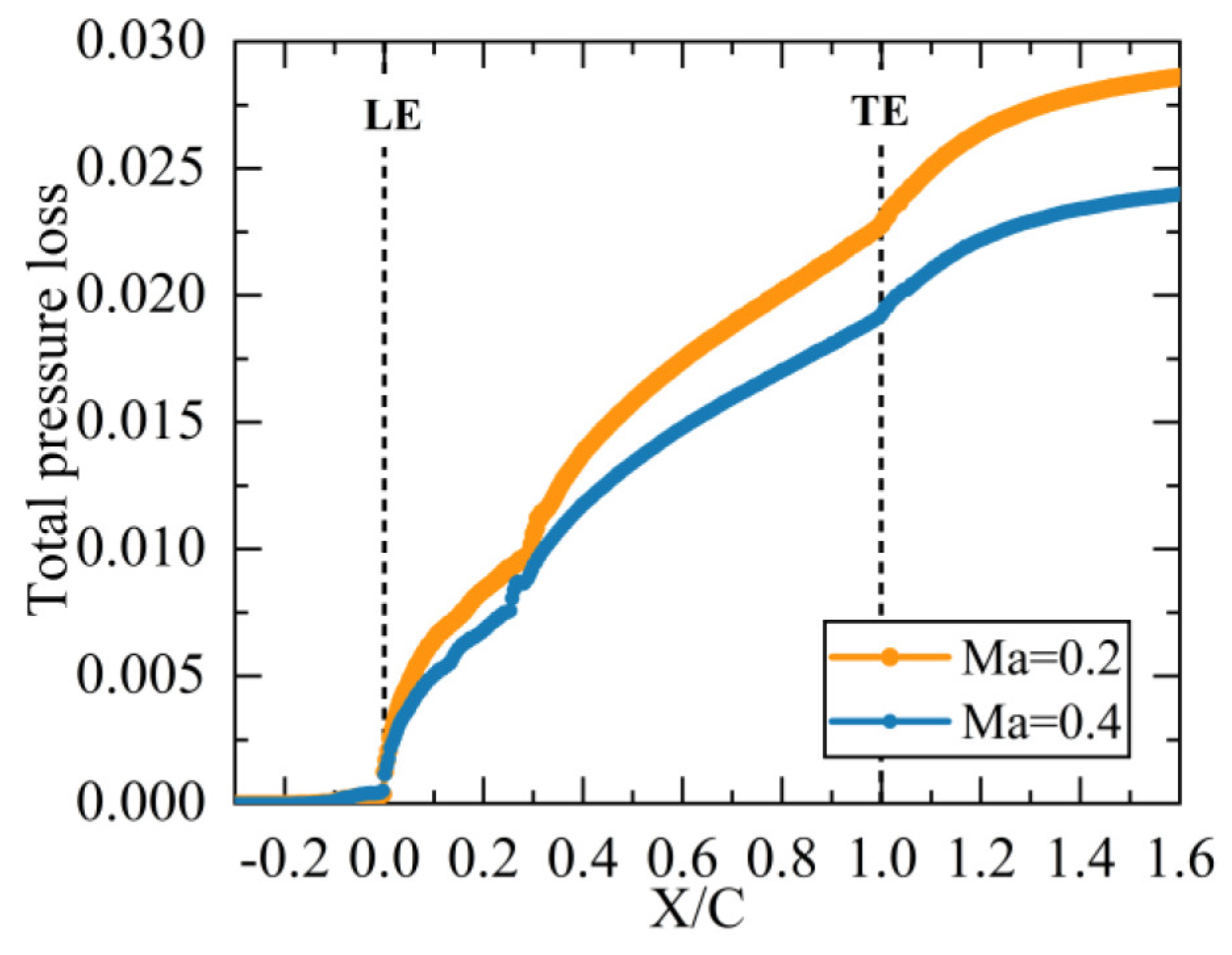
The dissipation factor can intuitively display the local loss situation, and the cumulative effect of the loss can be analyzed by studying the distribution of the total pressure loss along the flow direction, as shown in
Figure 21. The total pressure loss of the flow is nearly 0 before the leading edge of the blade and gradually increases after the leading edge due to the existence of friction loss. When the flow is separated at approximately 30% of the chord length, the total pressure loss increases in a small range. After the trailing edge of the profile, the turbulent dissipation increases due to the confluence of two flows from the suction and pressure surfaces, which accelerates the total pressure loss.


