Article

Self-Docking Characteristics and Sliding Mode Control on Space Electromagnetic Docking Mechanism

1
School of Mechanical Engineering, University of Science and Technology Beijing, Beijing 100083, China
2
Beijing Institute of Spacecraft System Engineering, Beijing 100094, China
*
Author to whom correspondence should be addressed.
Machines 2023, 11(3), 332; https://doi.org/10.3390/machines11030332
Submission received: 13 December 2022 / Revised: 9 February 2023 / Accepted: 17 February 2023 / Published: 28 February 2023
(This article belongs to the Section Automation and Control Systems)

Abstract

:
Electromagnetic docking technology can realize the flexible docking and safe separation of spacecraft, and presents broad application prospects. However, an electromagnetic force with nonlinearity and uncertainty properties increases the difficulties of the electromagnetic docking control. In this work, the magnetic dipole far-field model of a single coil has been established by simplifying the electromagnetic docking device. Afterward, the electromagnetic force and electromagnetic torque models were obtained during space electromagnetic docking. The space electromagnetic docking dynamics model was established by analyzing the influences of disturbance force and disturbance torque caused by a geomagnetic field. According to the one-dimensional docking reference trajectory, the sliding mode variable structure controllers based on exponential reaching law were proposed and verified. The quasi-sliding mode control method has been adopted to solve the chattering problem in sliding mode variable structure control. The simulation results show that it is necessary to design and add an electromagnetic controller to achieve flexible docking. The sliding mode variable structure controller based on quasi sliding mode can realize one-dimensional electromagnetic flexible docking, and have made good tracking effect on the reference trajectory. Compared with the control method based on exponential reaching law, it can reduce the chattering phenomenon in the control process. The sliding mode variable structure control strategy based on quasi sliding mode presented good robustness. Therefore, it can provide theoretical guidance and control reference for the flexible docking process between electromagnetic satellites.

1. Introduction

Space rendezvous and docking technology has been developed for more than 50 years. During this period, a variety of large docking mechanisms have been established such as probe-cone, androgynous peripheral assembly system (APAS), and a common berthing mechanism (CBM) [1]. For the International Space Station, these docking forms are still retained: the U.S. module uses the APAS, and the Russian module uses the probe-cone [1]. However, these mechanisms are connected with contact collision. With the rapid development of the on-orbit service, modular spacecraft have attracted more attention [2]. In spacecraft modular research, the design of an orbital replaceable unit (ORU) has been proposed worldwide. The ORU can be replaced and upgraded in orbit. It can also be used for the consumable replenishment and other operations, thus effectively extending the service life of the target spacecraft. Various studies have been carried out on ORUs such as the standard interface for robotic manipulation of payloads in future space missions (SIROM) [3], harmonized system study on interfaces and the standardization of fuel transfer ASSIST [4], and autonomous micro-satellite docking system (AMDS) [5]. Most of the docking mechanisms, whether spacecraft or ORU, realize the docking process through contact collision. Meanwhile, propellants employed in the traditional rendezvous and docking cause fuel consumption, optics pollution, plume impact, heat emissions, and other issues.
Electromagnetic docking technology is a new type of rendezvous and docking technology, which presents the advantages of no fuel consumption, no docking impact, and the effective prevention of plume pollution to optical elements [6]. NASA’s Miniature Autonomous Extravehicular Robotic Camera (Mini AERCam, NASA, Washington, DC, USA) achieves the transformation of electromagnet attraction and repulsion by controlling the direction of current [7]. The Massachusetts Institute of Technology (MIT) has raised the concept of electromagnetic formation flight (EMFF) [8]. The device for controlling EMFF is composed of three coils arranged orthogonally with each other [8]. The Reconfigurable Space Telescope of Autonomous Assembly was developed by researchers from the University of Surrey where the precise docking of multiple satellites was accomplished by coils and permanent magnets [9], and McGill University designed a cubic electromagnetic spacecraft called Tryphons [10]. The development of an electromagnetic docking mechanism makes the flexible docking of spacecraft possible.
Electromagnetic spacecraft uses electromagnetic force and torque to achieve flexible docking. However, the control on the electromagnetic force and torque has become a major difficulty due to nonlinearity and uncertainty [11]. Many efforts have been made for this difficulty. MIT has established three electromagnetic coils models of near-field, mid-field, and far-field through Gaussian flux law, potential function, and the magnetic dipole model [11], which laid the foundation for the dynamic research and control strategy formulation of electromagnetic docking technology. Based on the above electromagnetic coil model, Kwon [12], Zhang [13], and Shi [6,14] researched the control of electromagnetic spacecraft formation flight. Huang [15,16,17] treated such an electromagnetic formation flight as a free multi-rigid-body system connected by the force element. The Kane method has been applied to develop a generalized 6-DOF dynamic model with internal forces accommodated [16]. Based on the linear system theory, the stability and controllability of the electromagnetic formation have been analyzed, and the coordinated trajectory planning of the electromagnetic formation flight has been realized [15,17]. As the satellite formation is constantly affected by the electromagnetic torque generated by the Earth’s magnetic field, an alternative solution to dipole polarity switching has been proposed by Fabacher [18], who avoided the building of angular momentum caused by the Earth’s magnetic field on both satellites. Zhang [19] established a dynamic model of spacecraft orbit correction by inertial propulsion and electromagnetic force coupling between spacecraft. Based on the establishment of the dynamics model, the concept of self-docking [20,21] has been raised, and the self-docking characteristics of electromagnetic spacecraft have been studied from both theoretical and simulation aspects.
During the final stage of self-docking, the velocity of the spacecraft increases sharply, which leads to a larger impact force in the spacecraft docking process [22,23,24,25,26]. In order to achieve flexible docking, scholars have further studied the electromagnetic control strategy. Ahsun [22] used nonlinear adaptive control to study the near-ground flight of electromagnetic formations, while Kwon [24] used two controllers to simulate the electromagnetic formation. Zhao [26] established a linearized model of the aircraft, and designed a controller based on robust control theory. Meanwhile, the robustness of the controller has been verified by simulation. Cai [27] designed an active disturbance rejection control scheme combined with feedforward and feedback. The scheme indicates good robustness under the conditions of external interference and sensor noise. Torisaka [28] developed a method for relative attitude control without reaction wheels for reconfigurable spatial structures, while Huang [29] proposed an adaptive reaching law based sliding mode control for the trajectory tracking of EMFF with actuator saturation. Liu [30], Zeng [31], and Cai [32] realized the tracking of spacecraft formation flight through sliding mode control. Sliding-mode control is based on the design of a high-speed switching control law that drives the system’s trajectory onto the sliding surface. The robustness of sliding-mode control can theoretically ensure perfect tracking performance, despite parameter or model uncertainties [30,31,32]. However, in real-time applications, the sliding surface is not rigorously known, which leads to a high control activity known as chattering [33]. Chattering will excite high-frequency dynamics, which could be the cause of severe damage to the electromagnetic docking mechanism.
Propellants employed in traditional rendezvous and docking cause fuel consumption, optics pollution, plume impact, heat emissions, and other issues. Therefore, electromagnetic rendezvous and docking, a new rendezvous and docking technology, has the advantages of no fuel consumption and no docking impact, effectively avoiding the pollution of optical elements caused by plume. However, the nonlinearity and uncertainty of electromagnetic force increase the difficulties of the electromagnetic docking control. In this work, the magnetic dipole far-field model of single coil in the three-dimensional space coordinates was established by simplifying the electromagnetic docking device. The electromagnetic force and electromagnetic torque models during space electromagnetic docking were obtained. The space electromagnetic docking dynamics model was established by analyzing the influences of disturbance force and disturbance torque caused by the geomagnetic field. According to the one-dimensional docking reference trajectory, sliding mode variable structure controllers based on exponential reaching law were proposed and verified and the quasi-sliding mode control method was adopted to solve the chattering problem in the sliding mode variable structure control. This research can provide theoretical guidance for electromagnetic force and torque calculation, while offering control references for flexible docking technology between spacecrafts.

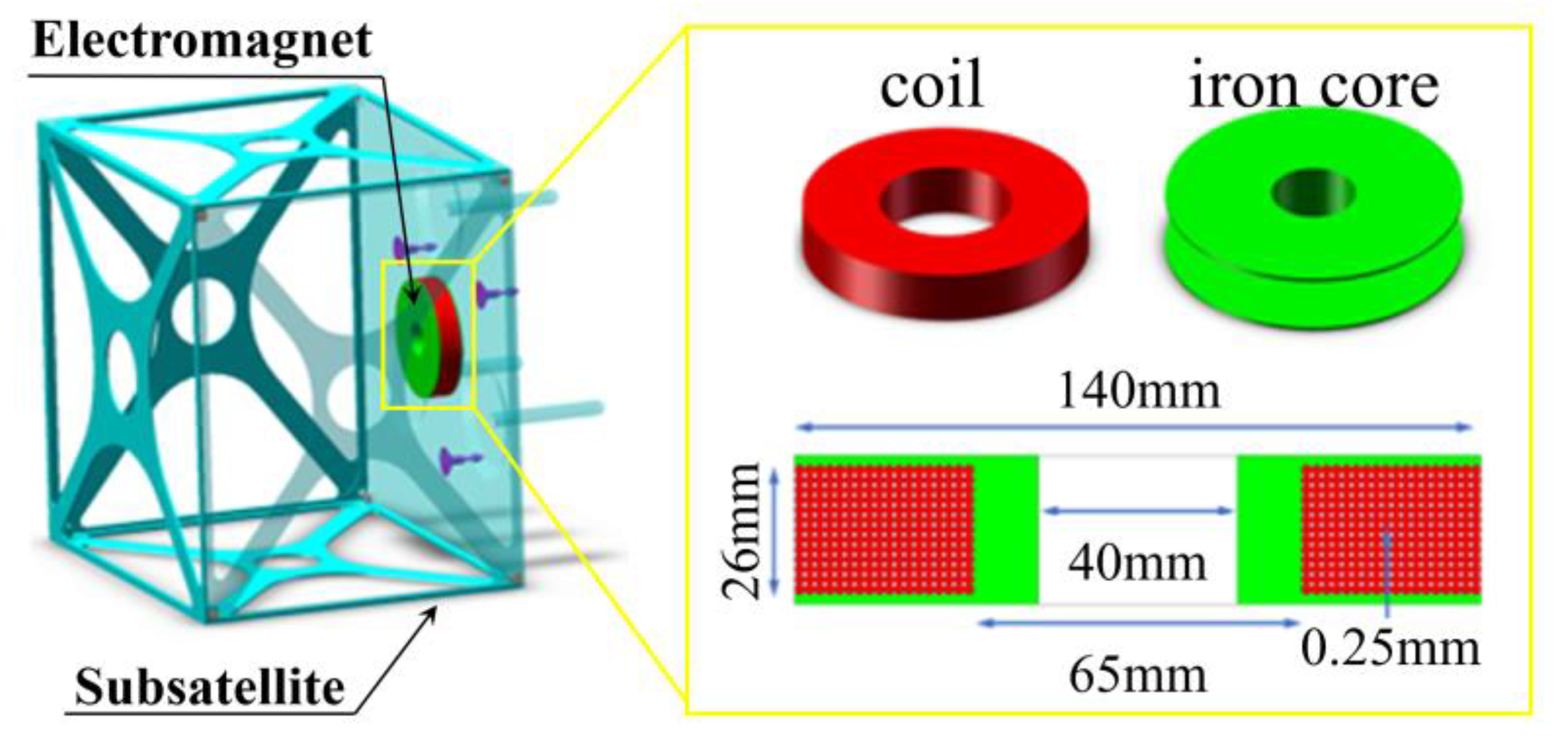
2. Mathematical Model of Electromagnetic Force and Torque in Space Electromagnetic Docking Process

The electromagnetic assisted docking mechanism studied in this work is composed of a coil and I-shaped iron core, as shown in Figure 1. Based on Maxwell software simulation, the geometric parameters of the coil and I-shaped iron core were determined on the basis of the comprehensive consideration of electromagnetic force, power, weight, and other parameters. The above contents can be obtained in the Supplementary Materials. The designed electromagnetic docking mechanism requires 3900 ampere turns, 113.8 W power, and a 2.86 kg weight.
In order to facilitate the discussion of the subsequent magnetic induction model, the coordinate system of the coil was defined first. The center of the coil was taken as the coordinate origin, and it was assumed that there was a counterclockwise current flowing inside the coil. The z-axis is collinear with the central axis of the coil and perpendicular to the plane where the coil is located. The direction of the z-axis is vertical upward. The x-axis coincides with the plane of the coil and the direction is horizontal to the right. The y-axis is determined by the right-hand screw rule. The coordinate system is shown in Figure 2.
In three-dimensional space, the magnetic induction intensity generated by the coil in arbitrary space can be obtained by the Biot–Savart law [11], as shown in Equation (1).
B = L d B = L μ 0 I 4 π d l × r r 3
where μ0 and I are the permeability of the vacuum and coil current, respectively.
Taking Figure 2 as an example, point S is an arbitrary point on the coil, and point P is a point outside the coil. α, β, γ are the angles between the vector r p and the coordinate axis, respectively. φ is the angle between the vector r s and the x-axis. d l is the length microelement of point S after rotating around the z-axis. According to the coordinate relationship in Figure 2, the expressions of d l and r can be substituted into Equation (1). The component of the magnetic induction intensity of the coil at any point in space can be obtained by Equations (2)–(4).
B x = μ 0 I R 4 π L r p cos γ cos φ ( r p 2 + R 2 2 R r p cos α cos φ 2 R r p cos β sin φ ) 1.5 d φ
B y = μ 0 I R 4 π L r p cos γ sin φ ( r p 2 + R 2 2 R r p cos α cos φ 2 R r p cos β sin φ ) 1.5 d φ
B z = μ 0 I R 4 π L R r p cos α cos φ r p cos β sin φ ( r p 2 + R 2 2 R r p cos α cos φ 2 R r p cos β sin φ ) 1.5 d φ
where R is the coil radius.
Three types of electromagnetic force models are commonly used in the related research of electromagnetic force and torque models: near-field model, mid-field model, and far-field model [11]. The near-field model is an accurate model, which is applicable to arbitrary distance between spacecraft. However, the electromagnetic force and torque of the near-field model are represented by a series of double integral equations, and it is difficult to obtain an analytical solution. For space electromagnetic docking, the distance between two spacecraft is usually greater than the radius of the electromagnetic coil. When the distance between two electromagnetic coils is far greater than the coil radius, the electromagnetic force and torque they suffer in each other’s magnetic field depends on the magnetic moment of the electromagnetic coil. The far-field model simplifies the energized coil as an electromagnet, and the electromagnet is modeled as a magnetic dipole. The approximate analytical solution of the electromagnetic force and torque can be derived by linearizing the near-field model with Taylor’s first-order expansion. The far-field model is applicable to the case where the distance between spacecraft is greater than the radius of the electromagnetic coil. The expressions of the electromagnetic force and the torque of the far-field model are simpler and do not contain integral equations, so it can be applied to the corresponding theoretical research and control methods.
Equations (2)–(4) can be expanded by using the McLaughlin formula, and the far-field model commonly used in the research of electromagnetic control strategy can be obtained [11]. The required McLaughlin formula is as follows:
( 1 + x ) a = 1 + a 1 ! x + a ( a 1 ) 2 ! x 2 + a ( a 1 ) ( a 2 ) 3 ! x 3 + o ( x 3 )
1 1 - x = 1 + x + x 2 + x 3 + o ( x 3 )
For the far-field model, McLaughlin’s formula was used to perform Taylor’s first-order expansion of the integral term where the approximate analytical solution of the electromagnetic force and torque can be derived. By employing Equations (5) and (6), the common integral term in Equations (2)–(4) can be Taylor expanded. The expanded form is shown in Equation (7).
1 ( r p 2 + R 2 2 R r p cos α cos φ 2 R r p cos β sin φ ) 1.5 = 1 r p 3 + 3 R cos α cos φ r p 4 + 3 R cos β sin φ r p 4
The common integral term in Equations (2)–(4) can be expanded by using Taylor’s first-order expansion. The component of the magnetic induction intensity of the coil at any point in space can be simplified by Equations (8)–(10) to facilitate the establishment of subsequent expressions of electromagnetic force and electromagnetic torque.
B x = 3 μ 0 I 1 π R 1 2 4 π x z ( x 2 + y 2 + z 2 ) 2.5
B y = 3 μ 0 I 1 π R 1 2 4 π y z ( x 2 + y 2 + z 2 ) 2.5
B z = μ 0 I 1 π R 1 2 4 π 2 z 2 x 2 y 2 ( x 2 + y 2 + z 2 ) 2.5
The far-field model simplifies the energized coil to an electromagnet and models the electromagnet as a magnetic dipole. According to the assumed current direction in Figure 2, the N pole direction of the magnetic dipole can be obtained through Ampere’s law. In order to ensure the consistency of the discussion before and after, the N-pole direction of the magnetic dipole is taken as the z-axis direction of the coordinate system. Taking the center of magnetic dipole 1 as the origin of coordinates, the z-axis is in the same direction as the N pole of magnetic dipole 1. The x-axis coincides with the plane of magnetic dipole 1 and the direction is horizontal to the right. The y-axis is determined by the right-hand screw rule. Similarly, the global coordinate system of magnetic dipole 2 (right) was established. The global coordinate systems between the two the magnetic dipoles are shown in Figure 3.
A single coil can be simplified into a magnetic dipole model. When the current is applied, the angle of two coils can be offset under the action of electromagnetic force and torque. The body coordinate systems can be established with the offset coils. The angle transformation relationship between the body coordinate systems and the global coordinate systems is shown in Figure 3a, and the vector relationship between the two coils is presented in Figure 3b. Based on the far-field model, the magnetic induction intensity component at an arbitrary point in space can be obtained with Equations (8)–(10). According to the Ampere force formula and the conservation of angular momentum, the scalar expressions of electromagnetic force and torque between the two coils can be calculated. The detailed calculation process is as follows.
According to the Ampere force formula, in the global coordinate system o-xyz, the electromagnetic force of coil 2 from coil 1 can be obtained by Equation (11).
F 12 = L 2 d f 12 = L 2 I 2 d l 2 × ( L 1 μ 0 I 1 4 π d l 1 × r 12 r 12 3 ) = L 2 I 2 d l 2 × B 12
The electromagnetic torque of coil 2 is the cross product of the arm and the electromagnetic force, as shown in Equation (12).
M 12 = L 2 r 2 s × d f 12
According to Newton’s Third Law of Motion, the electromagnetic force on coil 1 is shown in Equation (13) below.
F 21 = F 12
Since the system is not acted by external force and torque, the angular momentum between the coils is conserved, as shown in Equation (14).
M 21 + M 12 + r 31 × F 21 + r 32 × F 12 = 0
According to the coordinate relationship in Figure 2, the expressions of each vector are substituted into Equations (8)–(12). The high-order terms in the integral formula are omitted, and the far-field model of the electromagnetic force and torque can be obtained on the coils, as shown in Equations (15)–(20).
F 12 x = 3 μ 0 μ 1 μ 2 4 π d 4 ( 2 cos ξ 1 cos ξ 2 cos ( θ 1 θ 2 ) sin ξ 1 sin ξ 2 )
F 12 y = 3 μ 0 μ 1 μ 2 4 π d 4 ( cos ξ 1 sin ξ 2 sin θ 2 + sin ξ 1 cos ξ 2 sin θ 1 )
F 12 z = 3 μ 0 μ 1 μ 2 4 π d 4 ( cos ξ 1 sin ξ 2 cos θ 2 + sin ξ 1 cos ξ 2 cos θ 1 )
M 12 x = μ 0 μ 1 μ 2 4 π d 3 sin ξ 1 sin ξ 2 sin ( θ 2 θ 1 )
M 12 y = μ 0 μ 1 μ 2 4 π d 3 ( sin ξ 1 cos ξ 2 cos θ 1 + 2 cos ξ 1 sin ξ 2 cos θ 2 )
M 12 z = μ 0 μ 1 μ 2 4 π d 3 ( sin ξ 1 cos ξ 2 sin θ 1 + 2 cos ξ 1 sin ξ 2 sin θ 2 )
where μ0 is the permeability of vacuum; μ1 is equal to I 1 π R 1 2 ; and μ2 is equal to I 2 π R 2 2 .
The electromagnetic force and torque of coil 2 can be given by general expressions. According to Equations (13) and (14), the electromagnetic force and torque of coil 1 can be obtained accordingly.

3. Self-Docking Characteristics of Space Electromagnetic

3.1. Analysis of the Interference Effect from the Geomagnetic Field

Since the satellite studied in this paper is relatively close to the Earth, its orbit altitude is 500 km. The geomagnetic field can be regarded as a magnetic dipole model. In the docking process based on electromagnetic technology, electromagnetic devices may be affected by the interference of the geomagnetic field. Therefore, it is necessary to analyze the electromagnetic force and torque from the geomagnetic field.
In order to evaluate the influence of the geomagnetic field on the electromagnetic-assisted docking process, the electromagnetic force and torque between the satellite and the sub-satellite, the Earth and the sub-satellite were calculated, respectively. According to the design parameters of the coil, the magnetic torque of the coil (μ1 = μ2) is 32.18 A·m2, the distance between the sub-satellite and the center of the Earth (d) is 6.871 × 10⁶ m, the permeability of vacuum (μ0) is 4π × 10−7 T·m/A, and the magnetic torque of the geomagnetic field (μe) is approximately 7.79 × 10²² A·m2. Two ideal conditions were assumed here to calculate the electromagnetic force and electromagnetic torque, respectively. The first is the working condition without tolerance; ξ1, ξ2, θ1 and θ2 are all zero; and the two electromagnetic coils are parallel to each other at this time. The second is the working condition with angle deviation, ξ1 and ξ2 are equal to zero, θ1 and θ2 are equal to 3°; at this time, coil 1 and coil 2 have an angle of 3° in the y–z plane, respectively. The electromagnetic force and torque expression between satellites can be known by Equations (15)–(20). Since the two satellites begin to capture and dock at a distance of 0.3 m, the curve of electromagnetic force and torque during the docking process can be shown in Figure 4.
It can be seen from Figure 4a,b, that as the distance was reduced, the electromagnetic force and torque between the two satellites increased nonlinearly. The difference in the electromagnetic force and torque between the main satellite–subsatellite and the Earth–subsatellite increases. At a distance of 0.3 m, the electromagnetic force between the main satellite and the subsatellite was 7.67 × 10⁻² N, while the electromagnetic force between the Earth and the subsatellite was 6.75 × 10⁻¹⁰ N. The electromagnetic forces were quite different, so the interference force from the geomagnetic field could be ignored during the docking process. At a distance of 0.3 m, the electromagnetic torque between the main satellite and the subsatellite was 4.01 × 10⁻⁴ N·m, while the electromagnetic torque between the Earth and the subsatellite was 8.08 × 10⁻⁵ N·m, which was a difference of five times. As the axial distance between the satellite and the sub-satellite decreased, the difference between the two increased nonlinearly. When the axial distance between the satellite and the sub-satellite was 0.1 m, the electromagnetic torque between the satellite and the sub-satellite was 134 times greater than that between the Earth and the sub-satellite. Therefore, during the docking process between the satellite and the sub-satellite, the influence of the interference torque of the geomagnetic field can also be ignored.

3.2. Electromagnetic Self-Docking Characteristics

In order to study the self-docking characteristics of the electromagnetic docking device, the electromagnetic force and torque during the electromagnetic docking process were derived by the far-field model. Meanwhile, the interference of the Earth’s magnetic field could be ignored through comparative analysis. Therefore, during the docking process, the space electromagnetic docking device is only affected by electromagnetic force and torque. For satellites and sub-satellites, the mass of the satellite is much greater than that of the sub-satellites. Taking the research object of this paper as an example, the mass of the satellite was eight times that of the sub-satellite. To facilitate the solution, the docking process can be regarded as a process in which the main satellite is fixed, while the subsatellite moves.
Within time element t, the electromagnetic force and torque of the subsatellite is approximately constant. The linear acceleration, linear velocity, linear displacement, angular acceleration, angular velocity, and angular displacement of the subsatellite can be expressed as Equations (21)–(26) below.
a = F m
v = v 0 + a t
s = v 0 t + 1 2 a t 2
α = M J
w = w 0 + α t
θ = w 0 t + 1 2 α t 2
where F is the electromagnetic force of subsatellite; m is the subsatellite mass; v0 is the initial velocity of subsatellite; M is the electromagnetic torque received by subsatellite; and w0 is the initial angular velocity of subsatellite. To avoid repetition of the moment of inertia symbol and current symbol I; the symbol J has been used in Equation (24) to represent the moment of inertia of the subsatellite.
In this work, the maximum mass of the subsatellite and electromagnetic assisted docking device was about 20 kg. For subsatellites carrying different equipment, their mass and centroid distribution are different. In order to simplify the calculation, an ideal working condition was assumed, and the electromagnetic assisted docking device was regarded as a homogeneous body with a mass of 20 kg. The moment of inertia can be obtained from the geometric parameters of the coil, where Jx = 0.0525 kg·m2 and Jy = Jz = 0.0263 kg·m2.
Two working conditions were considered here to calculate the electromagnetic force and electromagnetic torque, respectively. The first is the working condition without tolerance; ξ1, ξ2, θ1, and θ2 are all zero; and the two electromagnetic coils are parallel to each other at this time. The second is the working condition with angular tolerance; ξ1, ξ2, and θ1 are equal to zero; and θ2 is equal to 3°, at this time, there is an angle of 3° between coil 2 and the y–z plane. Under the two working conditions above, the electromagnetic force and torque of coil 2 (subsatellite) can be calculated by Equations (15)–(20). The time microelement was taken as 0.001 s, and the initial docking velocity of the subsatellite was zero. Through the calculation of Equations (21)–(26), the simulation result curves of the linear displacement, linear velocity, angular displacement, and angular velocity of subsatellite during the docking process can be obtained, as shown in Figure 5 and Figure 6.
Under the conditions of no tolerance and a certain angle tolerance, the space electromagnetic assisted docking mechanism showed good self-docking characteristics. When two satellites were docked without tolerance, the distance between two satellites was reduced from 0.3 m to 0 m through the simulation of 8092-time steps, as shown in Figure 5a. Since the subsatellite is not subjected to electromagnetic force and torque in other directions, there is only a linear velocity along the x-axis, as shown in Figure 5b. When the subsatellite is docked with an angular tolerance of 3°, through the simulation of 8095-time steps, the distance between two satellites was reduced from 0.3 m to 0 m, as shown in Figure 6a. During this period, since the subsatellite was under little electromagnetic force along the z-axis, the linear displacement and linear velocity along the z-axis were nearly zero. The subsatellite was also subjected to electromagnetic torque around the y-axis. Under this torque, the angular displacement of the subsatellite constantly changed, and the angular tolerance in the final stage was close to 0.5°, as shown in Figure 6c. Regardless of whether there was an angle tolerance between the two satellites or not, the space electromagnetic assisted docking mechanism showed good self-docking characteristics. The position and attitude of the subsatellite can be adjusted to the alignment state through electromagnetic force and torque. During the simulation process of the two working conditions, the displacement and velocity of the subsatellites changed slowly in the early stage. However, at the end of the docking process, due to the nonlinear increase in the electromagnetic force and torque, the velocity of the subsatellite also increased. Higher speeds will result in the greater impact force of the collision between the subsatellite and the main satellite. Therefore, it is necessary to design and add an electromagnetic active controller to achieve a weak impact docking effect.

4. The Strategy of Sliding Mode Variable Structure Control

4.1. Design of Reference Trajectory for Non-Tolerance Docking Process

In order to achieve weak impact docking, it is necessary to limit the speed of the sub-satellite during the docking process. The reference trajectory for the sub-satellite’s movement was designed, as shown in Figure 7. During the docking process, the reference trajectory of the sub-satellite was set to accelerate first, then at a constant speed, and then decelerate. The initial reference speed of the sub-satellite was V0, the maximum reference speed was limited to Vm, and the final docking speed was zero, which can meet the requirements of flexible docking.
The initial linear velocity of the subsatellite (v0) was 0.001 m/s, the acceleration period (t1) was 20 s, the uniform velocity period (t2) was from 20 s to 30 s, the deceleration period (t3) was from 30 s to 40 s, and the initial distance between the two satellites (x0) was 0.3 m. After calculation and post-processing, the reference displacement, linear velocity, and acceleration curve of subsatellite are shown in Figure 8. By comparing Figure 8b and Figure 5b, there was no end-stage acceleration process in the velocity change curve of the one-dimensional docking reference trajectory, which is conducive to the realization of flexible docking. It also provides a mathematical model for the development of a sliding mode variable structure control strategy.

4.2. The Strategy of Sliding Mode Variable Structure Control Based on Exponential Reaching Law

In order to ensure that the sub-satellite can achieve flexible docking with the satellite according to the reference trajectory, it is necessary to study the control strategy of the electromagnetic-assisted docking mechanism. Sliding-mode control was based on the design of a high-speed switching control law that drives the system’s trajectory onto the sliding surface. The robustness of sliding-mode control can theoretically ensure perfect tracking performance, despite parameter or model uncertainties. In this section, a sliding mode variable structure control based on exponential reaching law was further designed and verified.
The exponential approach law [33,34] is expressed in Equation (27) below.
s ˙ = ε sgn ( s ) k s , ε > 0 , k > 0
where ε and k are a constant.
sgn(s) is a sign function [34], its expression is shown in Equation (28).
sgn ( s ) = { 1 s > 0 0 s = 0 1 s < 0
The dynamic equation of the subsatellite in the electromagnetic docking process is shown in Equation (29).
m x ¨ r e = 3 μ 0 μ 1 μ 2 2 π x r e 4 = 3 π μ 0 N 2 R 4 I 1 I 2 2 x r e 4
where μ0 is the permeability of vacuum; μ1 is equal to I 1 π R 1 2 ; and μ2 is equal to I 2 π R 2 2 .
The expression of the control system can be transformed from Equation (28), which is presented in Equation (30).
x ¨ r e = f ( x r e , t ) + g ( x r e , t ) u + d ( t )
where f ( x r e , t ) is 0; g ( x r e , t ) is 3 π μ 0 N 2 R 4 I 1 2 m x r e 4 ; d ( t ) is external interference, and its absolute value is less than or equal to D .
The switching function is developed as Equation (31).
s ( t ) = c e + e ˙
where c is a constant.
The theoretical reference position of the subsatellite, which is relative to the main satellite, is xr. During the docking process, the position error of the subsatellite can be expressed as Equation (32).
e = x r x r e
From Equations (29)–(32), Equation (33) can be obtained.
s ˙ ( t ) = c ( x ˙ r x ˙ r e ) + x ¨ r f ( x r e , t ) g ( x r e , t ) u d ( t )
Equation (27) is equal to Equation (33). The expression of the control function is shown in Equation (34).
u = ε sgn ( s ) + k s + c ( x ˙ r x ˙ r e ) + x ¨ r f ( x r e , t ) d ( t ) g ( x r e , t )
In a control system, it is difficult to know the changing law of external interference. Therefore, the control function was set with a predetermined interference limit. The absolute value of external interference was less than or equal to D, so Equation (34) can be transformed into Equation (35).
u = ε sgn ( s ) + k s + c ( x ˙ r x ˙ r e ) + x ¨ r f ( x r e , t ) D g ( x r e , t )
Substituting Equation (35) into Equation (33), Equation (36) can be achieved.
s ˙ ( t ) = ε sgn ( s ) k s + D d ( t )
Assuming that the maximum and the minimum values of external interference are dU and dL, the value of D is required to meet lim s 0 s s ˙ < 0 .
(1) When s ( t ) > 0 , s ˙ ( t ) = ε k s + D d ( t ) . In order to keep lim s 0 s s ˙ < 0 , D = d L .
(2) When s ( t ) < 0 , s ˙ ( t ) = ε k s + D d ( t ) . In order to ensure lim s 0 s s ˙ < 0 , D = d U .
Here, d 1 = d U + d L 2 and d 2 = d U d L 2 , D can be expressed as Equation (36).
D = d 1 d 2 sgn ( s )
In this section, a sliding mode variable structure control based on exponential reaching law was further designed and verified. Equations (27)–(37) describe the above control system strategy. The control system was designed by the switching function (Equation (31)) and control function (Equation (35)). The sliding mode control can be realized by using the exponential reaching law of sign function. The initial parameters were set as follows: the coefficient of isokinetic term (ε) in the exponential reaching law was 1 × 10⁻⁴, the coefficient of exponential term (k) was 5. The permeability of vacuum (μ0) was 4π × 10−7 T·m/A. The total number of turns of coil of the satellite (N) was 1.56 × 10⁴, and the effective radius (R) was 5.125 × 10⁻² m. The wire current of the coil on the main satellite (I1) was 0.1 A. The coefficient of switching function (c) was 10. The minimum value of external interference (dL) was −1 × 10⁻⁶, and the maximum value (dU) was 1 × 10⁻⁶. The external interference in the actual system is complex and unknown, thus the non-interfering ( d ( t ) = 0 ) and sinusoidal interference conditions ( d ( t ) = d U sin ( 2 π t ) ) were assumed. The simulation results under different interferences can be obtained through MATLAB programming calculation. The verification of the sliding mode variable structure control based on exponential reaching law can be found in Section 5.1.

4.3. The Strategy of Sliding Mode Variable Structure Control Based on Quasi Sliding Mode

In order to reduce the chattering phenomenon, the quasi-sliding mode method with saturation function (Equation (38)) was applied to carry out the sliding mode control during the docking process. The sign function (Equation (28)) was replaced by the saturation function. The difference between the two functions is the path through the origin neighborhood. The sign function directly transitions from −1 to 1 at the origin, while the saturation function transitions through a straight line with a slope path in the origin neighborhood.
s a t ( s ) = { 1 s > Δ s Δ | s | Δ 1 s < Δ
where Δ is the boundary layer and is a constant.
Replacing the sgn(s) by sat(s), the quasi-sliding mode with saturation function can realize the sliding mode control with initial parameters. When Δ = 0.01 and the other parameters are unchanged, the simulation results under different interferences can be found in Section 5.2.

5. Results and Discussion

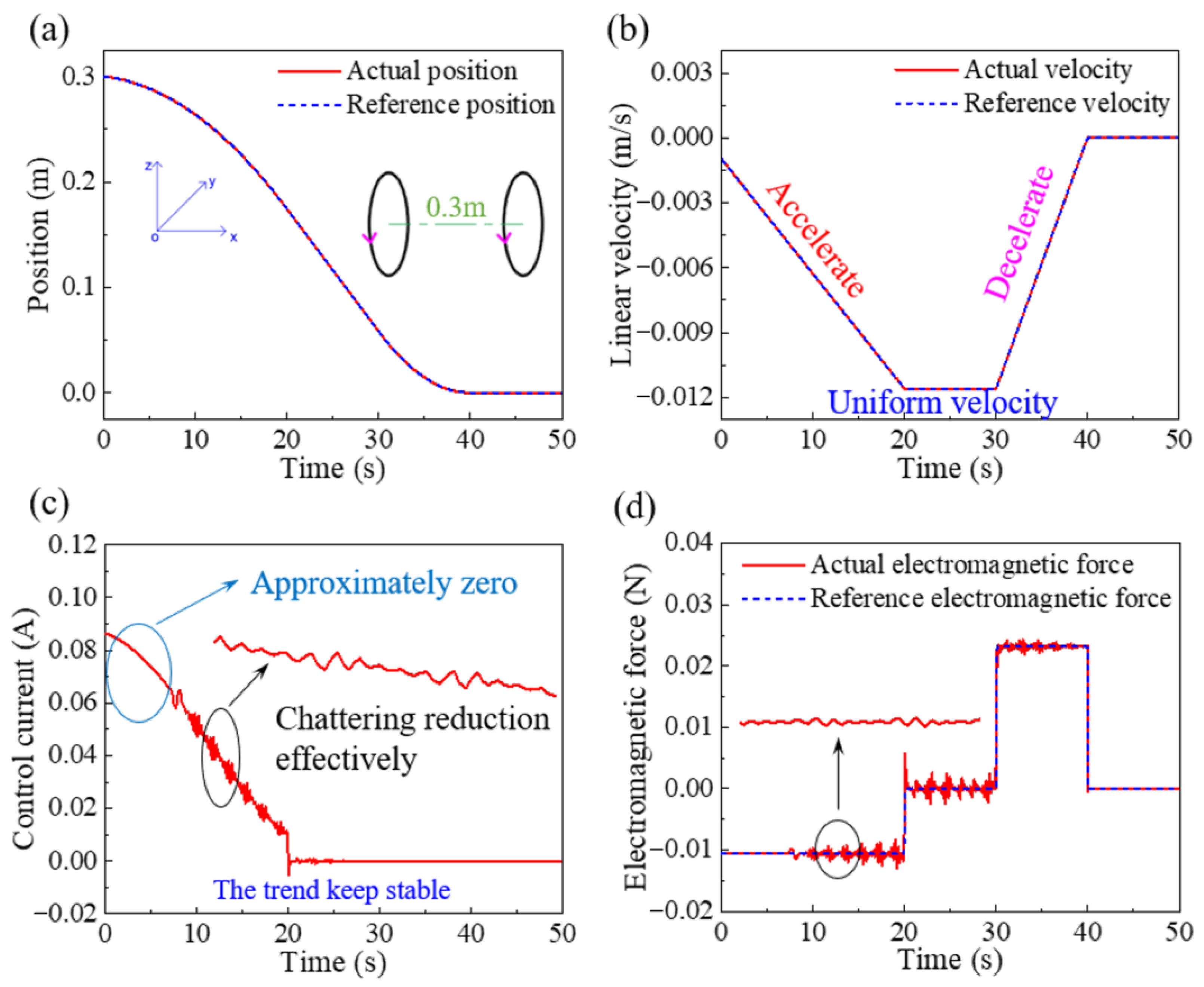
5.1. The Verification of Sliding Mode Variable Structure Control Based on Exponential Reaching Law

According to the sliding mode variable structure control based on the exponential approach law, the docking characteristics of the subsatellites under the non-interfering and sinusoidal interference conditions were studied, and the results are shown in Figure 9 and Figure 10. Figure 9a,b shows the position and linear velocity changes of the subsatellite along the x-axis. For the non-interference condition, the actual position and linear velocity change curves of the subsatellite were consistent with the reference position and linear velocity change curves. The above phenomena show that the sliding mode variable structure control based on the exponential reaching law had a good tracking effect. Figure 9c shows the variation in the coil current in the subsatellite. During the acceleration and uniform velocity stages, both two electromagnetic coils had the same direction of current. As the relative position of subsatellite and main satellite decreased, the control current of the subsatellite also decreased. During the deceleration stage, the current directions of two electromagnetic coils were the opposite, and the control current of subsatellite also gradually decreased. During the whole docking process, the chattering phenomenon of current in the subsatellite was obvious. The current range was 0.05 A. Due to the current change, the electromagnetic force of the subsatellite fluctuated around the reference electromagnetic force, as shown in Figure 9d.
For the sinusoidal interference condition, the tracking effect of the actual position and linear velocity of the subsatellite on the reference value was also good, as shown in Figure 10 a,b. By comparing c,d in Figure 9 and Figure 10, respectively, after introducing sinusoidal interference, the trend of the control current and actual electromagnetic force was stable at the original state, which reflected the strong robustness of the sliding mode control. However, the control current and actual electromagnetic force obviously indicated a sinusoidal component, and the chattering phenomenon was still serious.

5.2. The Verification of Sliding Mode Variable Structure Control Based on Quasi Sliding Mode

To reduce the chattering phenomenon, the quasi-sliding mode method with saturation function was applied to carry out the sliding mode control during the docking process. The simulation results under the non-interfering and sinusoidal interference conditions are shown in Figure 11 and Figure 12. For the non-interfering and sinusoidal interference conditions, the tracks of the actual position and linear velocity of the subsatellite tightly followed the reference, as shown in Figure 11a,b and Figure 12a,b. The sliding mode variable structure control based on the quasi sliding mode indicated a good tracking effect. By comparing c,d of Figure 9, Figure 10, Figure 11 and Figure 12, respectively, the use of a saturation function did not affect the trend of the actual control current and electromagnetic force, but it can effectively reduce the chattering phenomenon in the docking process. For the sinusoidal interference condition, small chattering appeared in the control current and actual electromagnetic force between 0 and 7 s. For the sliding mode variable structure control based on the quasi-sliding mode, the chattering phenomenon during the docking process could be effectively reduced. The amplitude of current chattering was reduced by 80% from 0.05 A to 0.01 A.
To realize flexible docking between the satellite and the subsatellite, it is necessary to design and add an electromagnetic controller to achieve a flexible docking performance. By comparing the sliding mode variable structure control strategy based on the exponential reaching law and the quasi-sliding mode, it was found that the advantages of the sliding mode variable structure control based on the quasi-sliding mode were more obvious. For the sliding mode variable structure control based on the quasi-sliding mode, the tracks of the actual position and linear velocity of the subsatellite tightly followed the reference, and the chattering phenomenon during the docking process could be effectively reduced. Therefore, this control strategy can be applied to the electromagnetic active controller to achieve flexible docking. In real applications, the direct current or voltage of the satellite electromagnetic coil is usually set to a fixed value. The direct current or voltage of the subsatellite electromagnetic coil can be regulated by an electromagnetic active controller to generate a controllable electromagnetic attraction or repulsion.

6. Conclusions

In this work, the self-docking characteristics and sliding mode variable structure control of the space electromagnetic docking device were studied. Some of our obtained conclusions are presented as follows:
  • The electromagnetic force and electromagnetic torque models during electromagnetic docking were obtained based on the far-field model. The self-docking characteristics of the electromagnetic docking device were analyzed by using the established space electromagnetic docking dynamics model. It was necessary to design and add an electromagnetic controller to achieve flexible docking.
  • According to the designed one-dimensional docking reference trajectory, the sliding mode variable structure control was proposed. The sliding mode variable structure control based on the exponential reaching law and quasi sliding mode showed good tracking effects on the reference trajectory, and could realize one-dimensional electromagnetic flexible docking.
  • Compared with the control method based on exponential reaching law, the quasi sliding mode could effectively reduce the chattering phenomenon in the docking control process and presented good robustness. The sliding mode variable structure control with the quasi-sliding mode reduced the amplitude of current chattering by 80%, which was from 0.05 A to 0.01 A.

Supplementary Materials

The following supporting information can be downloaded at: https://www.mdpi.com/article/10.3390/machines11030332/s1, Figure S1: Variation curve of electromagnetic force (a) and power (b) with the mandrel diameter of the I-shaped iron core; Figure S2 Surface magnetic induction intensity of electromagnetic docking device; Figure S3 Variation curve of electromagnetic force (a) and weight (b) with the through-hole diameter of the I-shaped iron core; Figure S4 Structural parameters of electromagnetic docking device; Table S1: Design requirements for electromagnetic docking device.

Author Contributions

Conceptualization, B.W. (Boyu Wei), J.Z. and N.K.; Methodology, S.M. and J.Z.; Software, S.M. and B.W. (Boyu Wei); Validation, B.W. (Boyu Wei), B.W. (Bo Wang) and R.H.; Formal analysis, B.W. (Bo Wang); Investigation, B.W. (Bo Wang) and R.H.; Resources, N.K.; Data curation, B.W. (Boyu Wei); Writing—original draft preparation, S.M. and B.W. (Boyu Wei); Writing—review and editing, B.W. (Boyu Wei) and N.K.; Visualization, J.Z.; Supervision, N.K.; Project administration, N.K.; Funding acquisition, N.K. All authors have read and agreed to the published version of the manuscript.

Funding

This research was funded by National Key R&D Program of China, grant number 2022YFB3402800.

Data Availability Statement

Not applicable.

Conflicts of Interest

The authors declare no conflict of interest.

References

  1. Kang, Y.; Zhou, H.; Ma, S.; Gao, B.; Tan, L. Review of Spacecraft Exposed Payload Adapter Technology. Spacecr. Eng. 2019, 28, 104–111. [Google Scholar]
  2. Lu, Y.F.; Xie, Z.J.; Wang, J.; Yue, H.H.; Wu, M.; Liu, Y.W. A novel design of a parallel gripper actuated by a large-stroke shape memory alloy actuator. Int. J. Mech. Sci. 2019, 159, 74–80. [Google Scholar] [CrossRef]
  3. Vinals, J.; Urgoiti, E.; Guerra, G.; Valiente, I.; Esnoz-Larraya, J.; Ilzkovitz, M.; Franćeski, M.; Letier, P.; Yan, X.-T.; Henry, G.; et al. Multi-Functional Interface for Flexibility and Reconfigurability of Future European Space Robotic Systems. Adv. Astronaut. Sci. Technol. 2018, 1, 119–133. [Google Scholar] [CrossRef] [Green Version]
  4. Medina, A.; Tomassini, A.; Suatoni, M.; Aviles, M.; Solway, N.; Coxhill, I.; Paraskevas, I.S.; Rekleitis, G.; Papadopoulos, E.; Krenn, R.; et al. Towards a standardized grasping and refuelling on-orbit servicing for geo spacecraft. Acta Astronaut 2017, 134, 1–10. [Google Scholar] [CrossRef]
  5. Anthony, B.H.; Peter, T., Jr.; Jane, C.P.; Greg, A.R.; Gregory, J.W. Advancements in design of an autonomous satellite docking system. Proc. SPIE Spacecr. Platf. Infrastruct. 2004, 5419, 107–118. [Google Scholar] [CrossRef]
  6. Shi, K.K.; Liu, C.; Biggs, J.D.; Sun, Z.W.; Yue, X.K. Observer-based control for spacecraft electromagnetic docking. Aerosp. Sci. Technol. 2020, 99, 105759. [Google Scholar] [CrossRef]
  7. Steven, E.F.; Steve, D.; Nathan, H.; Jennifer, D.W. Application of the mini AERCam free flyer for orbital inspection. Proc. SPIE Spacecr. Platf. Infrastruct. 2004, 5419, 26–35. [Google Scholar] [CrossRef]
  8. Kong, E.M.C.; Kwon, D.W.; Schweighart, S.A.; Elias, L.M.; Sedwick, R.J.; Miller, D.W. Electromagnetic formation flight for multisatellite arrays. J. Spacecr. Rocket. 2004, 41, 659–666. [Google Scholar] [CrossRef]
  9. Underwood, C.; Pellegrino, S.; Lappas, V.J.; Bridges, C.P.; Baker, J. Using CubeSat/micro-satellite technology to demonstrate the Autonomous Assembly of a Reconfigurable Space Telescope (AAReST). Acta Astronaut 2015, 114, 112–122. [Google Scholar] [CrossRef] [Green Version]
  10. Abouzakhm, P.; Sharf, I. Guidance, Navigation, and Control for Docking of Two Cubic Blimps. IFAC-PapersOnLine 2016, 49, 260–265. [Google Scholar] [CrossRef]
  11. Schweighart, S.A.; Sedwick, R.J. Explicit Dipole Trajectory Solution for Electromagnetically Controlled Spacecraft Clusters. J. Guid Control Dynam. 2010, 33, 1225–1235. [Google Scholar] [CrossRef]
  12. Kwon, D.W. Propellantless formation flight applications using electromagnetic satellite formations. Acta Astronaut. 2010, 67, 1189–1201. [Google Scholar] [CrossRef]
  13. Zhang, C.; Huang, X.L. Angular-Momentum Management of Electromagnetic Formation Flight Using Alternating Magnetic Fields. J. Guid. Control Dynam. 2016, 39, 1292–1302. [Google Scholar] [CrossRef]
  14. Shi, K.K.; Liu, C.; Sun, Z.W. Constrained fuel-free control for spacecraft electromagnetic docking in elliptical orbits. Acta Astronaut. 2019, 162, 14–24. [Google Scholar] [CrossRef]
  15. Huang, H.; Yang, L.P.; Zhu, Y.W.; Zhang, Y.W. Collective trajectory planning for satellite swarm using inter-satellite electromagnetic force. Acta Astronaut. 2014, 104, 220–230. [Google Scholar] [CrossRef]
  16. Huang, H.; Yang, L.; Zhu, Y.; Zhang, Y. Dynamics and relative equilibrium of spacecraft formation with non-contacting internal forces. Proc. Inst. Mech. Eng. Part G J. Aerosp. Eng. 2014, 228, 1171–1182. [Google Scholar] [CrossRef]
  17. Huang, H.; Zhu, Y.W.; Yang, L.P.; Zhang, Y.W. Stability and shape analysis of relative equilibrium for three-spacecraft electromagnetic formation. Acta Astronaut. 2014, 94, 116–131. [Google Scholar] [CrossRef] [Green Version]
  18. Fabacher, E.; Lizy-Destrez, S.; Alazard, D.; Ankersen, F.; Profizi, A. Guidance of magnetic space tug. Adv. Space Res. 2017, 60, 14–27. [Google Scholar] [CrossRef] [Green Version]
  19. Zhang, Y.W.; Yang, L.P.; Zhu, Y.W.; Huang, H. Dynamics and Solutions for Multispacecraft Electromagnetic Orbit Correction. J. Guid. Control Dynam. 2014, 37, 1604–1610. [Google Scholar] [CrossRef]
  20. Zhang, Y.W.; Yang, L.P.; Zhu, Y.W.; Ao, H.J.; Qi, D.W. Self-docking analysis and velocity-aimed control for spacecraft electromagnetic docking. Adv. Space Res. 2016, 57, 2314–2325. [Google Scholar] [CrossRef]
  21. Zhang, Y.W.; Yang, L.P.; Zhu, Y.W.; Ren, X.H.; Huang, H. Self-docking capability and control strategy of electromagnetic docking technology. Acta Astronaut. 2011, 69, 1073–1081. [Google Scholar] [CrossRef]
  22. Ahsun, U.; Miller, D.W.; Ramirez, J.L. Control of Electromagnetic Satellite Formations in Near-Earth Orbits. J. Guid. Control Dynam. 2010, 33, 1883–1891. [Google Scholar]
  23. Zhang, Y.W.; Yang, L.P.; Zhu, Y.W.; Huang, H. Dynamics and nonlinear control of space electromagnetic docking. J. Syst. Eng. Electron. 2013, 24, 454–462. [Google Scholar] [CrossRef]
  24. Kwon, D.W.; Sedwick, R.J.; Lee, S.I.; Ramirez-Riberos, J.L. Electromagnetic Formation Flight Testbed Using Superconducting Coils. J. Spacecr. Rocket. 2011, 48, 124–134. [Google Scholar] [CrossRef]
  25. Zhang, Y.W.; Yang, L.P.; Zhu, Y.W.; Huang, H.; Cai, W.W. Nonlinear 6-DOF control of spacecraft docking with inter-satellite electromagnetic force. Acta Astronaut. 2012, 77, 97–108. [Google Scholar] [CrossRef]
  26. Zhao, W.; Underwood, C. Robust transition control of a Martian coaxial tiltrotor aerobot. Acta Astronaut. 2014, 99, 111–129. [Google Scholar] [CrossRef]
  27. Cai, W.W.; Yang, L.P.; Zhu, Y.W.; Zhang, Y.W. Formation keeping control through inter-satellite electromagnetic force. Sci. China Technol. Sci. 2013, 56, 1102–1111. [Google Scholar] [CrossRef]
  28. Torisaka, A.; Ozawa, S.; Yamakawa, H.; Kobayashi, N. Control of Electromagnetic Current at Final Docking Phase of Small Satellites. J. Space Eng. 2013, 6, 44–55. [Google Scholar] [CrossRef] [Green Version]
  29. Huang, X.L.; Zhang, C.; Lu, H.Q.; Li, M.M. Adaptive reaching law based sliding mode control for electromagnetic formation flight with input saturation. J. Frankl. I 2016, 353, 2398–2417. [Google Scholar] [CrossRef]
  30. Liu, H.; Li, J.F.; Hexi, B.Y. Sliding mode control for low-thrust Earth-orbiting spacecraft formation maneuvering. Aerosp. Sci. Technol. 2006, 10, 636–643. [Google Scholar] [CrossRef]
  31. Zeng, G.Q.; Hu, M. Finite-time control for electromagnetic satellite formations. Acta Astronaut. 2012, 74, 120–130. [Google Scholar] [CrossRef]
  32. Cai, W.W.; Yang, L.P.; Zhu, Y.W.; Zhang, Y.W. Optimal satellite formation reconfiguration actuated by inter-satellite electromagnetic forces. Acta Astronaut. 2013, 89, 154–165. [Google Scholar] [CrossRef]
  33. Fallaha, C.J.; Saad, M.; Kanaan, H.Y.; Al-Haddad, K. Sliding-Mode Robot Control With Exponential Reaching Law. IEEE Trans. Ind. Electron. 2011, 58, 600–610. [Google Scholar] [CrossRef]
  34. Weibing, G.; Hung, J.C. Variable structure control of nonlinear systems: A new approach. IEEE Trans. Ind. Electron. 1993, 40, 45–55. [Google Scholar] [CrossRef]
Figure 1. Schematic diagram of the electromagnetic assisted docking mechanism.
Machines 11 00332 g001
Figure 2. Establishment of the coordinate system.
Machines 11 00332 g002
Figure 3. The angular relationship between the global coordinate systems and the body coordinate systems (a) and the vector relationship between the coils (b). The distance between the centers of two magnetic dipoles is expressed by d.
Machines 11 00332 g003
Figure 4. The electromagnetic force (a) and torque (b) of the main satellite–subsatellite, and the Earth–subsatellite.
Machines 11 00332 g004
Figure 5. The linear displacement (a), linear velocity (b), angular displacement (c), and the angular velocity (d) of the subsatellite during the docking process with non-tolerance.
Machines 11 00332 g005
Figure 6. The linear displacement (a), linear velocity (b), angular displacement (c), and angular velocity (d) of the subsatellite during the docking process with a tolerance of 3°.
Machines 11 00332 g006
Figure 7. The one-dimensional docking reference trajectory of “acceleration—uniform velocity—deceleration” for the subsatellite.
Machines 11 00332 g007
Figure 8. The reference displacement (a), linear velocity (b), and acceleration (c) of the subsatellite.
Machines 11 00332 g008
Figure 9. The position (a), linear velocity (b), control current (c), and electromagnetic force (d) of the sliding mode control based on exponential reaching law with the non-interfering condition.
Machines 11 00332 g009
Figure 10. The position (a), linear velocity (b), control current (c), and electromagnetic force (d) of the sliding mode control based on exponential reaching law with sinusoidal interference.
Machines 11 00332 g010
Figure 11. The position (a), linear velocity (b), control current (c), and electromagnetic force (d) of the sliding mode control based on the quasi sliding mode with the non-interfering condition.
Machines 11 00332 g011
Figure 12. The position (a), linear velocity (b), control current (c), and electromagnetic force (d) of the sliding mode control based on the quasi sliding mode with sinusoidal interference.
Machines 11 00332 g012
Disclaimer/Publisher’s Note: The statements, opinions and data contained in all publications are solely those of the individual author(s) and contributor(s) and not of MDPI and/or the editor(s). MDPI and/or the editor(s) disclaim responsibility for any injury to people or property resulting from any ideas, methods, instructions or products referred to in the content.

