Higher-Order Hexahedral Finite Elements for Structural Dynamics: A Comparative Review

Abstract

The finite element method (FEM) is widely used in many engineering applications. The popularity of FEM led to the development of several variants of formulations, and hexahedral meshes surged as one of the most computationally effective. After briefly reviewing the reasons and advantages behind the formulation of increasing order elements, including the serendipity variants and the associated reduced integration schemes, a systematic comparison of the most common hexahedral formulations is presented. A numerical benchmark was used to assess convergency rates and computational efficiencies when solving the eigenvalue problem for linear dynamic analysis. The obtained results confirmed the superior performances of the higher-order brick element formulations. In terms of computational efficiency, defined as the ratio between achievable accuracy and computational execution time, quadratic or cubic formulations exhibited the best results for the stages of FE model assembly and solution computation, respectively.

1. Introduction

In many fields of science and engineering, the application of the fundamental principles of physics often leads to the formulation of the system model in the form of partial differential equations (PDEs). Therefore, obtaining an accurate numerical solution for PDEs in a timely manner is crucial. The finite element method (FEM) has been affirmed over the last decades as one of the most widely used methodologies. Based on the Galerkin formulation, FEM allows dealing effectively with the weak form of the PDEs [1].

Because FEM is numerical, thus an approximated methodology, several criteria need to be met in order to obtain stability, convergence, and accuracy of the results [2,3,4]. Accuracy ensures the limitation of the deviations of the approximated solution from the exact behavior within prescribed levels of tolerance. Stability criteria are used to ensure that desired levels of accuracy are met robustly, thus within tolerance over the whole domain, and irrespective of subtle variations of the FE solution parameters. Unstable solutions may arise as the result of multiple reasons, such as a poor choice of the approximating functions, a “bad” domain discretization, or an incorrect representation of the boundary conditions. Convergence criteria define the relationships between the mesh size and the achieved accuracy, thus focusing on measuring how the discretization error diminishes with the decreasing characteristic mesh size, hence with an increasing number of degrees of freedom. The results of the convergence studies can be used to derive guidelines for setting the optimal element size for a given finite element type, allowing for the saving a considerable amount of computational effort, as shown in [5] for the simulation of Lamb waves.

The error estimation approaches for studying the accuracy of numerical methods can be classified into two categories [6]. On the one hand, a-priori estimates rely on the knowledge of the asymptotic law representing the specific order of convergence [7]. On the other hand, a-posteriori estimation techniques focus more on pollution error, which arises due to the accumulation of the effects of the dispersion errors distributed over the whole domain [8].

Mitigation of dispersion errors is notably achieved by using a finer mesh but also by adopting higher-order finite elements [9]. The hp-version adaptive finite element algorithm represents adaptive mesh refinement with increasing polynomial order. An hp-algorithm was proposed in [10] to determine the eigen solutions of moderately thick cylindrical shells, involving the issues of variable geometrical factors, such as the thickness, circumferential wave number, radius, and length.

When using linear meshes to capture events of increasing frequency, the number of elements needed to mitigate interpolation, especially pollution errors, increases more than linearly, posing significant limitations on the use of such elements for modeling highly dynamic applications [11]. Therefore, among the above-mentioned alternatives, higher-order elements inherently possess a faster convergence, although at the expense of an increased computational cost [11,12,13]. One way to overcome problems related to the computational burden was proposed in [14] through a matrix-free approach applied to higher-polynomial shape functions used for fracture problems.

Several studies in the literature investigated the matter [15,16,17,18,19,20,21], but usually limiting the comparative analysis to spare groups of elements, such as the linear and quadratic hexa type only [15,16,17,21], or instead to just the serendipity elements [18,19,20]. Only a few works have investigated cubic elements, in most cases considering the cubic serendipity elements [22].

This paper proposes an extensive comparative analysis of the various brick element formulations, extended from the linear to the cubic order, also considering the serendipity variants. Moreover, the investigation is complemented by also considering Gauss–Legendre integration schemes with increasing order, as it affects both the accuracy and the computational efficiency of each FE formulation. A representative eigenproblem example containing different-order hexahedral elements with various numbers of integration points, was investigated to evaluate the accuracy and performance of FE formulations. High predictive accuracy of eigenvalues and eigenfunctions is crucial for reliable analyses in structural dynamics [23,24].

The remainder of the paper is outlined as follows: Section 2 summarizes the fundamental steps necessary to formulate a structural dynamic problem using FEM; Section 3 deals with the major challenges and numerical issues related to the art of obtaining a good-quality FE mesh. Section 4 focuses on the formulation of several types of hexahedral elements, also considering the serendipity variants. Comparative results of different orders and types of hexahedral elements are presented and discussed in Section 5. Concluding remarks are drawn in Section 6.

2. FE Formulation for Structural Dynamics Problems

FEM consists basically of the following steps: (1) formulating the variational integral form of the different contributions of the virtual work principle; (2) discretizing the domain by splitting it into a finite set of elements; (3) integrating the contributions of each element.

2.1. Variational Integral Form of the Virtual Work Principle

The equation of motion for an elastic body based on the standard variational statement of Hamilton’s principle is as follows [19]:

$$\underset{t_1}{\overset{t_2}{{\displaystyle \int }}}\left[\delta W_f+\delta T-\delta \Pi \right]dt=0,$$

(1)

where $W_f$ is the work performed by the external forces, T is the kinetic energy, and Π is the elastic strain energy.

The kinetic energy of the entire problem domain is defined in the following integral form:

$$T=\frac{1}{2}\underset{\Omega }{\overset{}{{\displaystyle \int }}}\rho {\dot{\mathit{u}}}^T\dot{\mathit{u}}d\Omega ,$$

(2)

where Ω represents the whole domain of the solid and $\dot{\mathit{u}}$ is the time-derivative of the displacement field.

The strain energy of an elastic solid can be expressed as follows:

$$\Pi =\frac{1}{2}\underset{\Omega }{\overset{}{{\displaystyle \int }}}{\mathit{\epsilon }}^T\mathsf{\sigma }d\Omega ,$$

(3)

where $\mathsf{\epsilon }$ and $\mathsf{\sigma }$ are the strain and the stress fields, respectively.

The work performed by the external forces is the sum of the contributions of surface forces $f_s$ and body forces $f_b$:

$$W_f=\underset{S_f}{\overset{}{{\displaystyle \int }}}{\mathit{u}}^{\mathit{T}}{f}_{\mathit{s}}d{S}_f+\underset{\Omega }{\overset{}{{\displaystyle \int }}}{\mathit{u}}^{\mathit{T}}{f}_{\mathit{b}}d\Omega ,$$

(4)

where $S_f$ represents the boundary surface of the body.

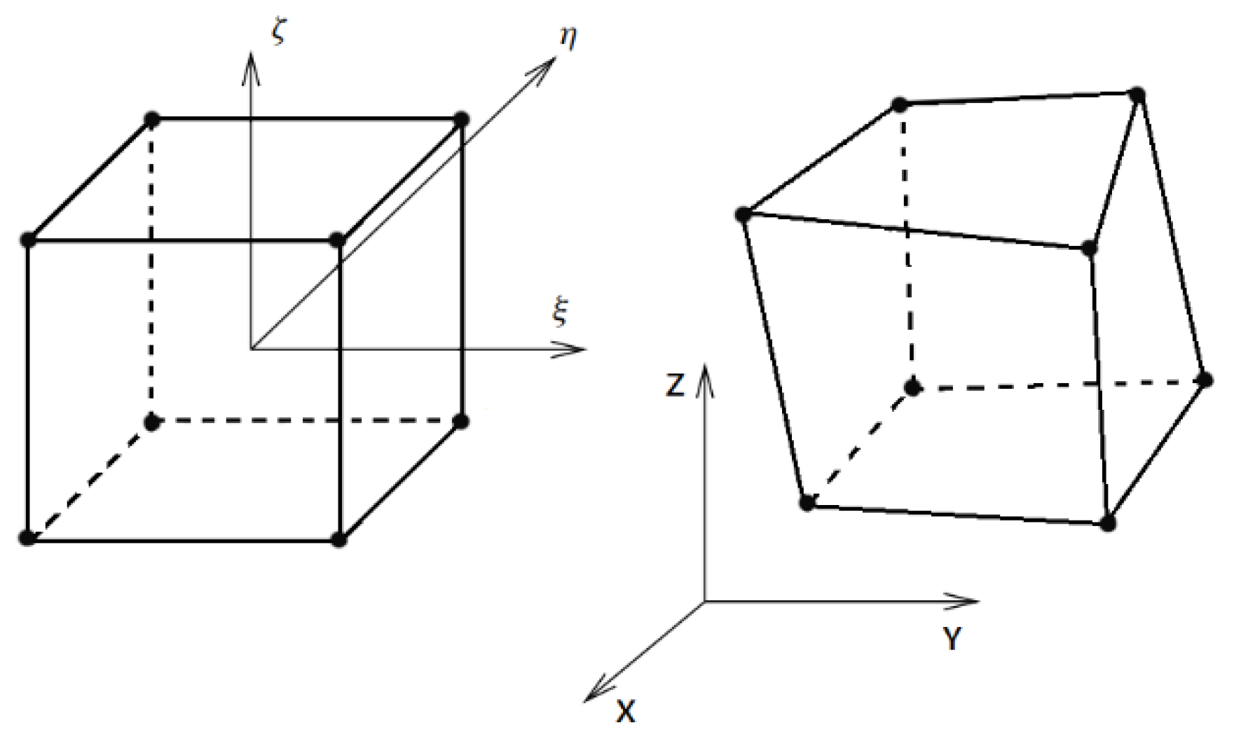
2.2. Spatial Discretization

The complexity of evaluating the integrals of Equations (2)–(4) is alleviated by splitting the domain of integration into finite elements. Within each element, the unknown displacement field, $\mathit{u}$, is approximated as the linear combination of a set of n interpolation functions, $N_i\left(\xi ,\eta ,\varsigma \right)$, also known as shapes functions [20]:

$$\mathit{u}=\left\{\begin{array}{c}{u}_x\\ u_y\\ u_z\end{array}\right\}= {\displaystyle \sum }_i\left[\begin{array}{ccc}{N}_i& & \\ & N_i& \\ & & N_i\end{array}\right]\left\{\begin{array}{c}{q}_x^i\\ q_y^i\\ q_z^i\end{array}\right\}=\left[\begin{array}{ccccccc}{N}_1& & & & N_n& & \\ & N_1& & \dots & & N_n& \\ & & N_1& & & & N_n\end{array}\right]\left\{\begin{array}{c}{q}_x^1\\ q_y^1\\ q_z^1\\ ⋮\\ q_x^n\\ q_y^n\\ q_z^n\end{array}\right\}=N\mathit{q}$$

(5)

where N is the matrix of the shape functions, q is the vector of nodal displacements, and $n$ is also the number of nodes defining the element.

Under the assumption of linear elasticity, the strain-stress relationship is governed by the following:

$$\mathit{\sigma }=D\mathit{\epsilon },$$

(6)

where the material characteristic matrix, $D$, is obtained as a function of the Poisson ratio, $\nu$, and of the Young’s modulus, $E$, as follows:

$$D=\frac{E}{\left(1+\nu \right)\left(1-2\nu \right)}\left[\begin{array}{cccccc}1-\nu & \nu & \nu & 0& 0& 0\\ \nu & 1-\nu & \nu & 0& 0& 0\\ \nu & \nu & 1-\nu & 0& 0& 0\\ 0& 0& 0& \left(1-2\nu \right)/2& 0& 0\\ 0& 0& 0& 0& \left(1-2\nu \right)/2& 0\\ 0& 0& 0& 0& 0& \left(1-2\nu \right)/2\end{array}\right].$$

(7)

For the purpose of formulating the FE problem, the differential operator, $\mathbf{\partial }$, is adopted in order to derive the strain field, $\mathbf{\epsilon }$, as a function of the nodal displacements vector, q:

$$\mathit{\epsilon }=\left\{\begin{array}{c}{\epsilon }_x\\ {\epsilon }_y\\ \begin{array}{c}{\epsilon }_z\\ {\gamma }_{xy}\\ \begin{array}{c}{\gamma }_{yz}\\ {\gamma }_{xz}\end{array}\end{array}\end{array}\right\}=\left(\begin{array}{ccc}\frac{\partial }{\partial x}& 0& 0\\ 0& \frac{\partial }{\partial y}& 0\\ 0& 0& \frac{\partial }{\partial z}\\ \frac{\partial }{\partial y}& \frac{\partial }{\partial x}& 0\\ 0& \frac{\partial }{\partial z}& \frac{\partial }{\partial y}\\ \frac{\partial }{\partial z}& 0& \frac{\partial }{\partial x}\end{array}\right)\left\{\begin{array}{c}{u}_x\\ u_y\\ u_z\end{array}\right\}=\mathsf{\partial }\mathit{u}=\mathsf{\partial }Nq=B\mathit{q}$$

(8)

As a result of Equation (8), and by using the material elasticity properties, both strain and stress fields can be formulated as functions of the nodal displacement q as follows:

$$\begin{array}{l}\mathit{\epsilon }=B\mathit{q}\hfill \\ \mathit{\sigma }=DB\mathit{q}\hfill \end{array}$$

(9)

where B is the strain displacement matrix, obtained by applying the differential operator to the shape function matrix.

The evaluation of integrals expressed in Equations (2)–(4) is reduced to a summation of the integral contributions of all the elements. Thanks to the expressions derived in Equations (5) and (9), for each element, the strain energy, ${\Pi }^e$; the kinetic energy, $T^e$, and the work performed by external forces, $W_f{}^e$, can be evaluated more easily, according to the following [19,21]:

$$\begin{array}{lll}{\Pi }^e=\frac{1}{2}\underset{{\mathsf{\Omega }}^e}{\overset{}{{\displaystyle \int }}}{\mathit{\epsilon }}^{\mathit{T}}\mathsf{\sigma } d\mathsf{\Omega }=\frac{1}{2} {\mathit{q}}^{\mathit{T}}\left(\underset{{\mathsf{\Omega }}^e}{\overset{}{{\displaystyle \int }}}{B}^{\mathit{T}}DB d\mathsf{\Omega }\right)\mathit{q}=\frac{1}{2} {\mathit{q}}^{\mathit{T}} K^e \mathit{q},\hfill & \hfill & K^e=\underset{{\mathsf{\Omega }}^e }{\overset{}{{\displaystyle \int }}}{B}^{{T}}DB d\mathsf{\Omega }\hfill \end{array}$$

(10)

$$\begin{array}{lll}{T}^e=\frac{1}{2}\underset{{\mathsf{\Omega }}^e}{\overset{}{{\displaystyle \int }}}\rho {\dot{\mathit{u}}}^{\mathit{T}}\dot{\mathit{u}} d\mathsf{\Omega }=\frac{1}{2}{\dot{\mathit{q}}}^{\mathit{T}}\left(\underset{{\mathsf{\Omega }}^e}{\overset{}{{\displaystyle \int }}}\rho N^{T}N d\mathsf{\Omega }\right)\dot{\mathit{q}}=\frac{1}{2}{\dot{\mathit{q}}}^{\mathit{T}}{M}^{\mathit{e}}\dot{\mathit{q},}\hfill & \hfill & M^{\mathit{e}}=\underset{{\mathsf{\Omega }}^e }{\overset{}{{\displaystyle \int }}}\rho N^T N d\mathsf{\Omega }\hfill \end{array}$$

(11)

$$\begin{array}{ccc}{W}_f{}^e=\underset{S^e}{\overset{}{{\displaystyle \int }}}{\mathit{u}}^{\mathit{T}}{\mathit{f}}_{\mathit{s}} dS+\underset{{\mathsf{\Omega }}^e}{\overset{}{{\displaystyle \int }}}{\mathit{u}}^{\mathit{T}}{\mathit{f}}_{\mathit{b}} d\mathsf{\Omega }={\mathit{q}}^{\mathit{T}}\left(\underset{S^e}{\overset{}{{\displaystyle \int }}}{N}^T{\mathit{f}}_{\mathit{s}} dS\right)+{\mathit{q}}^{\mathit{T}}\left(\underset{{\mathsf{\Omega }}^e}{\overset{}{{\displaystyle \int }}}{N}^T{\mathit{f}}_{\mathit{b}} d\mathsf{\Omega }\right)={\mathit{q}}^{\mathit{T}}{\mathit{F}}_{\mathit{s}}+{\mathit{q}}^{\mathit{T}}{\mathit{F}}_{\mathit{b}}={\mathit{q}}^{\mathit{T}}{\mathit{F}}^{\mathit{e}},& & \end{array}$$

(12)

$${\mathit{F}}^{\mathit{e}}=\underset{S^e}{\overset{}{{\displaystyle \int }}}{N}^T{\mathit{f}}_{\mathit{S}} dS+\underset{{\mathsf{\Omega }}^e}{\overset{}{{\displaystyle \int }}}{N}^T{\mathit{f}}_{\mathit{b}} d\mathsf{\Omega }$$

where the evaluation of the integrals leads directly to the formulation of the stiffness matrix, $K^e$, and the mass matrix, $M^e$, of the element. The surface integration is performed only for elements on the boundary of the problem domain. ${\mathit{F}}^{\mathit{e}}$ is the generalized force vector…

2.3. Numerial Integration Using Gauss–Legendre Quadrature

The computation of the stiffness and mass matrices, as well as of the load vector, requires the evaluation of a few definite volume integrals. Performing a good approximation by means of an adequate numerical quadrature procedure is crucial to the overall accuracy. A variety of approaches have been proposed in the field of numerical integration techniques [25]. The most common method of quadrature used within FE relies on the Gauss quadrature rules as follows: depending on the chosen integration order, the rule dictates the amount and location of a finite set of sampling points, as well as their corresponding weight. Exploiting the numerical integration scheme, the evaluation of the integrals in Equations (10)–(12) is approximated as the following weighted sums:

$$K^e\cong {\displaystyle \sum }_g{w}_g B_g{}^{T}D{B}_g\mathit{det}\left(J\right)$$

(13)

$$M^e\cong {\displaystyle \sum }_g{w}_g \rho N_g{}^T{N}_g\mathit{det}\left(J\right)$$

(14)

$${\mathit{F}}^{\mathit{e}}\cong {\displaystyle \sum }_g{w}_g N_g{}^T{\mathit{f}}_b\mathit{det}\left(J\right)+{\displaystyle \sum }_g{w}_g N_g{}^T{\mathit{f}}_s\mathit{det}\left(J\right)$$

(15)

where $w_g$ is the weight associated with the gth sampling point; J is the Jacobian matrix used to perform transformation from the local coordinate system $\left(\xi ,\eta ,\varsigma \right)$ of each element to the global cartesian system; $\rho$ is the material density.

Finally, the global mass and stiffness matrices, as well as the global force vector, are obtained by assembling the contributions of all the elements according to their connectivity [19,20].

2.4. Equations of Motion and Eigenvalue Problem

Exploiting the well-known Hamilton principle, Equations (1)–(15) pose the fundamentals to transform the weak form of the structural dynamic problem of Equation (1) into the following discretized second-order differential equation system [26]:

$$M\ddot{\mathit{q}}+K\mathit{q}=\mathit{F}$$

(16)

The accuracy of the solution to the considered dynamic problem is affected by the accuracy and correctness of the obtained matrices [27]. However, the correctness of transient analyses may also be influenced by the accuracy of the chosen time-integration scheme. For this reason, it is more robust to accomplish convergence studies of FE models by studying the associated eigenvalue problem for modal analysis. The free vibration problem is formulated as follows:

$$M\ddot{\mathit{q}}+K\mathit{q}=0,$$

(17)

which can be notably solved by posing the following generalized discrete eigenvalue problem:

$$K \mathit{\varphi }={\omega }^{2}M \mathit{\varphi }.$$

(18)

Solving Equation (18) results in obtaining m eigenvalue-eigenvector pairs $\left({\lambda }_k,{\mathit{\varphi }}_k \right), \mathrm{k}=1,\dots ,m$. Each eigenvector, also known as eigenmode, represents one mode shape of the freely vibrating system, while the square root of the corresponding eigenvalue is the associated vibration frequency, also known as eigenfrequency or natural frequency.

The effects of the arbitrary scaling of the eigenvectors obtained by solving Equation (18) by means of iterative procedures can be alleviated by assuming a normalization strategy. In this work, the mass-normalized convention for the mode shape was adopted, from which the following expressions of the orthogonality properties of the eigenmodes with respect to the mass and to the stiffness matrices derive:

$${\mathit{\varphi }}_{\mathit{k}}{}^{\mathit{T}}M{\mathit{\varphi }}_{\mathit{j}}={\delta }_{kj},$$

(19)

$${\mathit{\varphi }}_{\mathit{k}}{}^{\mathit{T}}\mathit{K}{\mathit{\varphi }}_{\mathit{j}}={\delta }_{kj}{\omega }_k^2.$$

(20)

2.5. Estimating the FE Accuracy for Dynamic Applications

To assess the quality of the FE solution, proper performance metrics must be defined and able to effectively capture the difference between a theoretically exact solution and the one provided by means of FEM [21]. As discussed in previous sections, the following two sources of approximation are introduced by FEM: the first source is the finite order of interpolation of the chosen shape functions, and the other one may arise from the use of Gauss–Legendre integration for the computation of the system matrices [20].

Modal parameters, such as the natural frequencies and mode shapes, characterize the linear dynamic properties of a vibrating structure and can be used to evaluate indirectly the accuracy of the stiffness and mass matrices obtained through FEM. In fact, studying the convergence behavior requests the evaluation of both eigenvalues and eigenvectors [17]. In another study, a different a priori criterion was proposed based on the evaluation of the maximum eigenvalue of the stiffness matrix [28].

Error estimation and mitigation techniques have been extensively researched in the literature [29,30]. In particular, studying the convergence rate aims to improve the mesh quality and obtain an optimal balance between accuracy and computational cost. The estimation of the convergence rate is oriented to find out an asymptotic behavior, upon which design choices can be empirically made for achieving results in viable terms, allowing obtaining an adequate accuracy level in a timely acceptable window [31]. As already stated in the introduction, the estimation of the error convergence rates relies on either a-priori or a-posteriori approaches [6].

Given a certain law of the convergence rate, one could a-priori perform a small set of preliminary FE analyses in order to capture its asymptotic behavior. For example, one option is to consider the convergence rate of the displacement error norm, E_u, which is known to follow the following linear trend:

$$E_u\cong Ch.$$

(21)

In this case, the asymptotic behavior can be estimated through linear regression, which results in obtaining the value of the constant $C$, as a function of the characteristic mesh size, h. The knowledge of C can be finally used to tune the mesh density according to the desired level of accuracy. As documented in [32], the convergence rate of the relative eigenvalue errors, ${\mathrm{E}}_{\lambda }$, is governed by the following exponential trend:

$${\mathrm{E}}_{{\lambda }_k}=\frac{{\lambda }_k^h-{\lambda }_k}{{\lambda }_k}\le c {\left(h {\lambda }_k\right)}^p,$$

(22)

where ${\mathsf{\lambda }}_{\mathrm{k}}^h$ and ${\mathsf{\lambda }}_{\mathrm{k}}$ represent the reference and approximated k-th eigenvalues, $p$ is the degree of the shape functions, and h is the characteristic mesh size.

In a simpler scenario, the a-posteriori error metric is defined and quantified in order to make an estimation of the actual accuracy of the obtained FE model [33]. Babuska and Rheinboldt [34] were among the first authors to propose a class of a-posteriori error estimations based on the inter-element discontinuity for the C0-continuous approximation of the solution field. Later, Zienkiewicz and Zhu [35] proposed a different error estimation focusing on stress field deviations. Other studies were dedicated to obtaining adaptive algorithms, which allow the generation of successive convergent solutions, for which the performance of the error indicators depends on both grid splitting and the choice of an order [36,37].

Several error metrics were proposed in order to assess objectively the accuracy caused by both the discretization and the integration approximations. Each metric is targeted to a particular need as follows: depending on the FE application, a different error norm may be used to minimize the deviations in terms of displacements, elastic energy, or stress [38,39,40]. Recently, Reali and Hughes [32] presented a comprehensive approach for estimating the error of FE approximations, demonstrating the existence of an intimate relationship between the relative errors in the eigenvalues, eigenmodes error norm, and energy norm, which applies to each eigenmode separately.

In the present work, starting from Equation (22), the mean relative eigenvalue error has been adopted as an accuracy metric.

3. Key Factors for a Good FE Formulation

As discussed in Section 2.2, the discretization stage consists in splitting the domain of the partial differential boundary problem, by means of a finite set of elements. Within each element, continuous field quantities are mapped to discrete nodal quantities by means of the dedicated interpolation functions, ${\mathrm{N}}_i$.

Notably, shape functions are derived to guarantee the following two properties: compatibility and completeness. Compatibility ensures the maintenance of a certain degree of continuity across the inter-element boundaries, whereas completeness refers to the capability of capturing rigid body motions as well as constant strain states [41].

Discretization errors arise from the difference between the true field quantities and the corresponding ones captured through the liner combination of the shape functions [29,42]. For example, errors in displacements arise by comparing the true displacement field, ${\mathit{u}}^h,$ with the approximated one, $\mathit{u}=N\mathit{q}$. Therefore, FE accuracy is strongly related to the shape functions and to their capability of fully representing the underlying physical phenomena.

More in general, particular care must be taken during the discretization phase to guarantee the accuracy and stability of the solution and avoid undesirable phenomena. The shear-locking behavior is among the most problematic challenges to cope with, as it can exhibit unphysically stiff responses [43]. Such behavior may happen when using too few linear elements along the thickness of a plate. As a result, locking phenomena will cause an underestimation of deflections and stresses, with a high risk of overwhelming safety margins during the design phase [44].

For these reasons, reduced integration schemes (RI) were introduced so that these “locking” phenomena disappear [45]. But the major drawback of these RI schemes is a mesh instability often known as “hourglassing” [46]. It often manifests, giving rise to unphysical zero-energy modes that are caused when the number of calculated zero eigenvalues exceeds the rigid body modes. It can lead to numerical instabilities and erroneous solutions due to the rank deficiency of the equations of motion [47,48,49]. Several techniques have been proposed to mitigate hourglassing effects. The first technique was developed by Belytschko, who proposed to enrich the model descriptions using ‘artificial damping’ and ‘artificial stiffness’ [50]. The B-bar method described in [51] can be applied to avoid spurious modes for the anisotropic and non-linear media. It relies on using a stabilization matrix, which does not contribute to any deformation modes except for the hourglass ones, thus ensuring the element passes the patch test [52]. To treat the spurious instability, special solution methods and various element formulations have been developed [53,54]. A new formulation, based on the 3D-MITC8 element, has been proposed to prevent both hourglassing and locking in [55].

Higher-order elements rely on a high-order polynomial expansion within each element. As a result, quadratic elements can capture bending and curvilinear shapes, providing an intrinsically superior robustness against hourglassing and incompatible modes [56,57]. Higher-than-second-order elements, such as cubic, quartic, and so on, may present even better performances in preventing shear locking. However, especially in combination with explicit solution methods, where the time increment size is related to nodal spacing, the usage of higher-order elements may demand unnecessary small-time integration steps [57].

As briefly discussed in the previous section, a-priori criteria can be used to guide the designer in performing a refinement of the mesh such that the accuracy of a FE model can be optimized. Mesh refinement is usually based on two different, but complementary strategies adopted to increase the accuracy [10]. On the one hand, h-refinement relies on the progressive reduction of the element size. The effects of element size on the accuracy of FE models were investigated through static, impact, and modal analyses in [58]. In [59], fully automatic hp-adaptivity is implemented for a 3D problem. H-adaptivity is also an effective tool to introduce local mesh refinement in the FEM-based numerical simulation of crack propagation and could be beneficial for the numerical simulation of fatigue or accidental load scenarios [60]. On the other hand, the p-refinement strategy relies on using a progressively increased order of the elements, thus increasing the polynomial order of their shape functions [61,62]. A complimentary approach to pure p-refinement strategy for an eight-node Hermitian hexahedral element was presented in [63], where authors considered six DOFs per node, three DOFs for the canonical displacements, and three extra DOFs to explicitly capture the local rotations. It is worth noting that higher-order elements possess the intrinsic capability of capturing rotational effects but without demanding for extra efforts required by an explicit representation of the rotational DOFs. The origin of the hp-adaptive approach, which is a combination of the former two methods, dates back to the works of Babuška et al. [64,65], who originally suggested that FEM converges exponentially when the mesh is refined by a suitable combination of both strategies.

4. Different Formulations of the Hexahedral (Brick) Element

Considering the importance of defining the shape functions correctly, a large number of studies have been dedicated for the investigation of defining several types of elements [19,20,21,22,66,67,68]. Among all types of solid elements, hexahedral (brick) modeling strikes a balance of meshing ease, accuracy, and efficiency [67,68].

Besides the hexahedral elements, tetrahedral elements are affirmed due to their superior ease of use in terms of the capability of adapting to curved shapes. However, hexahedral elements provide relatively higher accuracy, allowing for a lower mesh density, thus, for a better computational efficiency [69,70]. The lower accuracy of tetrahedral elements manifests more clearly, especially on the occasion of high deformation problems, such as nonlinear elasto-plastic analyses. For instance, even second-order tetrameshes underperform when compared to the ones obtained using linear brick elements when shear stress is dominant. Moreover, it is shown that in structural dynamics problems, different performances are found since tetrahedral elements tend to overestimate the model stiffness [17].

Despite the documented superior performance of brick elements with respect to tetrahedral ones, in some cases, it is still preferable to use both types leading to the necessity of transition elements, such as the prismatic and pyramidal ones. It is worth noting that all the solid elements, including the tetrahedral ones, can be easily formulated by “degeneration” of the eight-node hexahedron by collapsing two or multiple nodes.

The study presented here focused on comparing hexahedral elements with increasing order formulations up to the cubic one. Implementation details of all the considered formulations are reported in Appendix A. For all the considered formulations, the iso-parametric approach was adopted, thus using the same interpolating functions to approximate the state (displacements, strains, stresses, etc.) fields, as well as the geometry. The position vector of each point within an iso-parametric regular brick element can be transformed from the local coordinates $\left(\xi , \eta ,\zeta \right)$ that vary between −1 and 1 into the Cartesian (X,Y,Z) coordinates and vice versa.

4.1. Serendipity Brick Elements

As noted in [71], using higher-order elements will produce matrices with a larger bandwidth. As a consequence, denser sparse matrices will cause a corresponding decrease in computational performances.

A common solution used to alleviate the computational burden is represented by the serendipity elements [18,20,22,72,73,74], which are obtained from the regular ones by keeping only the nodes belonging to the edges, which are the only ones contributing to the inter-element C0 continuity connection. As a result, they provide similar accuracy to their regular counterparts while obtaining a considerable reduction in the number of DOFs, and, thus, in the size of the element matrices. This property could, in part, mitigate the computational disadvantage of obtaining denser matrices, which typically results from using higher-order elements.

This fact, in part, justifies the frequent integration of these kinds of elements in commercial FE software. Nevertheless, it is worth noting that although both serendipity and regular elements can achieve complete polynomial resolution, they do it with different degrees of completeness. For instance, second-order serendipity elements can fully represent first-order polynomials with the enrichment of a few quadratic terms, whereas regular quadratic elements fully represent the second-order polynomials.

The superiority of regular elements with respect to the serendipity alternatives was confirmed by studying the effects of element distortions on the displacement-based accuracy. The reported advantages are known to be significant in case of high distortion, which manifests clearly along the coarser-to-finer transition regions usually necessary to discretize complicated geometrical boundaries, such as in holes and corners [75,76].

The comparative analysis of this study was, therefore, complemented, including the quadratic and cubic serendipity elements. The implementation details are reported in Appendix A.

4.2. Under-Integration vs. Full-Integration Schemes

As anticipated in Section 2.3, Gauss quadrature allows the evaluation of the definite integrals, by means of a weighted sum of the integrand function over a set of interior points, referred to as sampling points. In the Gauss quadrature, the position of the sampling points and the corresponding weights are chosen so that a polynomial of a given degree can be integrated exactly. For a polynomial of degree 2m − 1, full integration is achieved if m sampling points and the corresponding weights are chosen according to the quadrature rule.

As mentioned in Section 4.1, when dealing with solids and structures with complicated loads or geometries, locking problems may arise. In [67], full-order integration of trilinear iso-parametric brick elements was shown to lead to locking phenomena. The use of reduced-integration schemes is known to be beneficial to mitigate the locking effects. In fact, the typical overestimation of the stiffness matrix can be balanced using fewer sampling points, which can generate a less stiff element [77].

5. Results and Discussion

This section discusses the results of the comparative numerical analysis of several C0 continuous hexahedral finite elements with the aim of assessing their computational efficiency and predictive accuracy. The considered formulations and the related integration schemes are detailed in

Table 1. Design of experiments.

		Integration Schemes
Order	Nodes	2 × 2 × 2	3 × 3 × 3	4 × 4 × 4
Linear	8	Hexa8-Int8
Quadratic Serendipity	20	Hexa20-Int8 1	Hexa20-Int27
Quadratic	27		Hexa27-Int27
Cubic Serendipity	32		Hexa32-Int27 1	Hexa32-Int64
Cubic	64			Hexa64-Int64

¹ Serendipity formulations with reduced integration.

.

As can be noted in Table 1, under-integration was considered only for the serendipity elements since under-integration of regular elements may lead to unstable results. Over-integration schemes, such as the Hexa8-Int27, Hexa8-Int64, Hexa20-Int64, and Hexa27-Int64, were not considered in this study, as they produce the same accuracy as the regular integration equivalents, but with deteriorating computational performances as documented in [56].

The numerical comparison has been conducted by studying the eigenvalue problem of a cube with size equal to 200 mm and clamped on one face, as depicted in Figure 1. The main mechanical properties of the considered model are detailed in

Table 2. Mechanical properties of the material.

Young’s Modulus E, GPa	Density ρ, kg/m3	Poisson’s Ratio ν
206.94	7829	0.288

.

As detailed in

Table 3. FE formulations considered in the comparative analysis.

Test Name	Shape Type	Integration Scheme	N. of Elements in All Directions
Hexa8-Int8	Linear	2 × 2 × 2	6	12	18	24	30	36
Hexa20-Int8 2	Quadratic	2 × 2 × 2	4	7	11	15	19	23
Hexa20-Int27	Quadratic	3 × 3 × 3	4	7	11	15	19	23
Hexa27-Int27	Quadratic	3 × 3 × 3	3	6	9	12	15	18
Hexa32-Int27 2	Cubic	3 × 3 × 3	3	6	9	12	15	18
Hexa32-Int64	Cubic	4 × 4 × 4	3	6	9	12	15	18
Hexa64-Int64	Cubic	4 × 4 × 4	2	4	6	8	10	12	14 1

¹ Referent mesh. ^2. Reduced integration serendipity elements.

, the following seven FE formulations were considered: the full-order linear, quadratic, and cubic brick elements, as well as their serendipity counterparts. For each considered FE formulation, the corresponding model was discretized using an increasing mesh density, as reported in Table 3. In particular, the increasing mesh density was tuned in order to maintain as much as possible a similar number of nodes, hence a similar number of degrees of freedom.

For each scenario, first, the mass and the stiffness matrices were assembled, then the associated eigenvalue problem was solved, by means of the Krylov-Schur algorithm [78], extracting the first ten modes. The accuracy was investigated considering the mean value of the relative eigenvalue errors, as defined in Equation (22). For the purposes of evaluating the errors, the solution obtained with a mesh of 2744 equally spaced cubic hexahedral elements was assumed as a reference. The results of this computation are reported in

Table 4. Natural frequencies and modal shapes of the first 10 modes computed for the reference model.

Mode 1 2732.90, Hz	Mode 2 2732.90, Hz	Mode 3 3730.90, Hz	Mode 4 6520.08, Hz	Mode 5 7244.23, Hz
Mode 6 7244.23, Hz	Mode 7 8944.78, Hz	Mode 8 10,599.78, Hz	Mode 9 11,034.94, Hz	Mode 10 11,267.65, Hz

.

All numerical evaluations were executed on a workstation featuring an 11th generation Intel^® Core™ i7-1165G7 2.80 GHz quad-core eight-thread processor and 16 GB of DDR4 3200 MHz RAM, running on Windows 10 operating system and assigning to the working process higher execution priority. The FE solutions were obtained using a dedicated in-house prototype implementation of the reported FE formulations. Being the prototype code not yet optimized, the reported computational times are not meant for an absolute comparison with otherwise available solutions, such as commercial software, but they still provide a useful insight into comparing the computational efficiency of the different formulations.

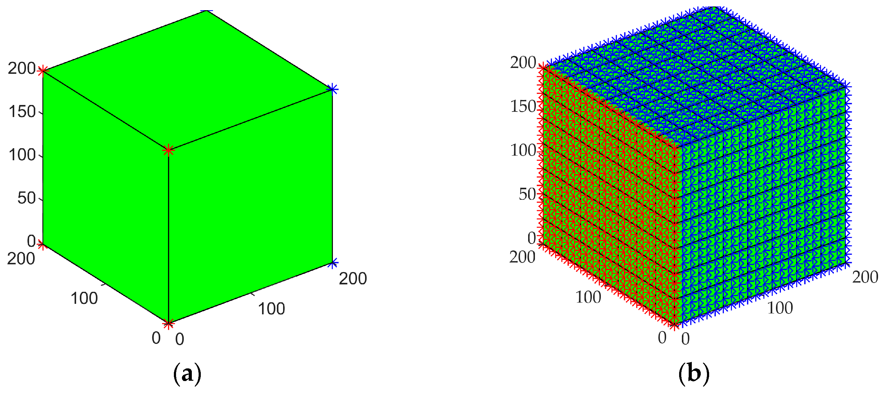
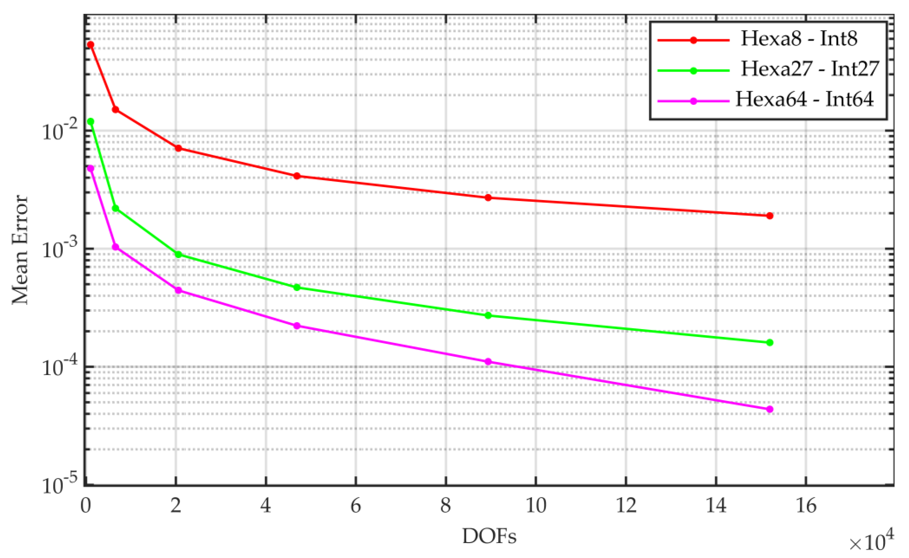
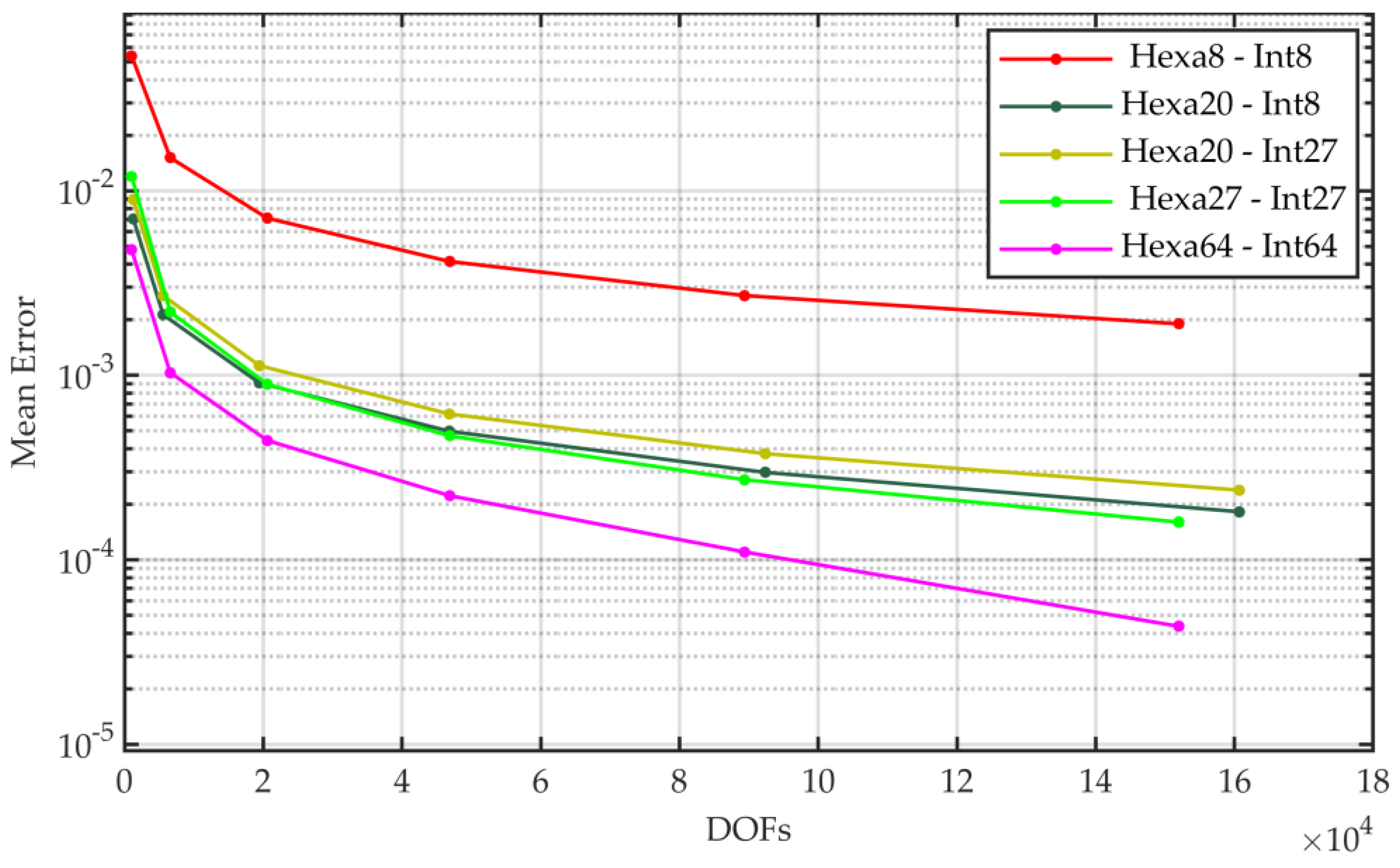
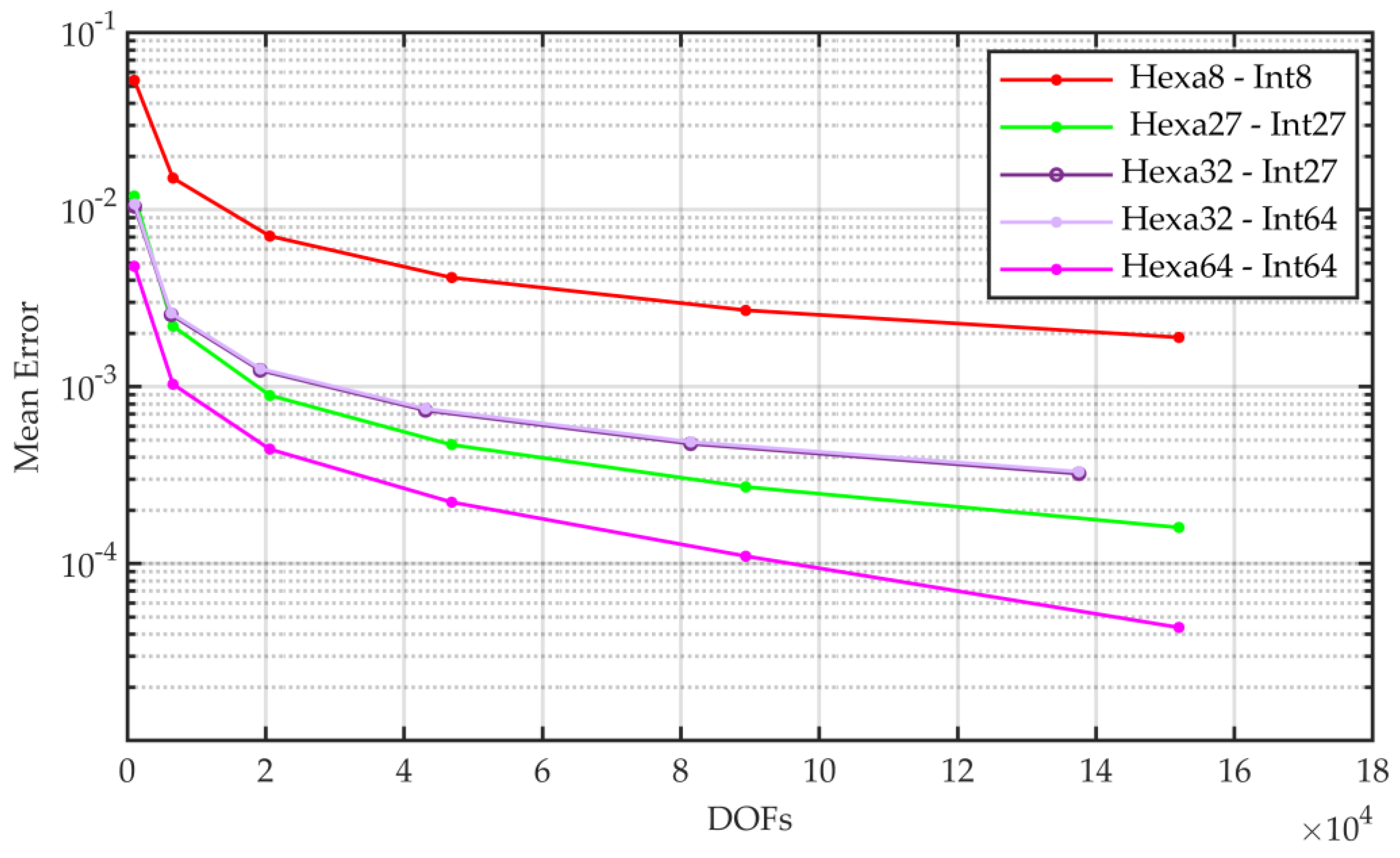
5.1. Accuracy Convergence

Figure 2 depicts the convergence accuracy curves of the full-order linear (hexa8-int8), quadratic (hexa27-int27), and cubic (hexa64-int64) hexahedral elements.

As expected, linear brick elements have the worse convergence rate. Quadratic elements perform much better, featuring a remarkable accuracy gain, as follows: above one order of magnitude at converge values. Finally, also cubic elements show further improvements with respect to quadratic ones, but less pronounced.

Figure 3 and Figure 4 expand the previous comparisons, respectively, to the quadratic and cubic serendipity elements, including the reduced integration variants. For the quadratic case (Figure 3), the serendipity element (Hexa20-Int27) shows a marginally slower convergence as compared to the full-order quadratic formulation. Moreover, as discussed in Section 4, the reduced integration exhibits the expected beneficial effects, making the corresponding serendipity formulation (Hexa20-Int8) as effective as the full-order one (Hexa27-Int27).

On the opposite, all cubic serendipity formulations underperform with respect to the quadratic formulation, indicating that there are no benefits in considering serendipity variants above the second order, even when using reduced integration schemes.

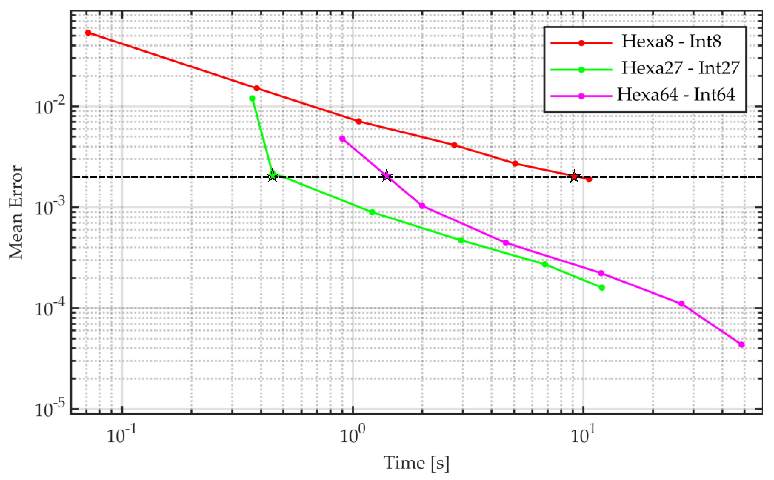
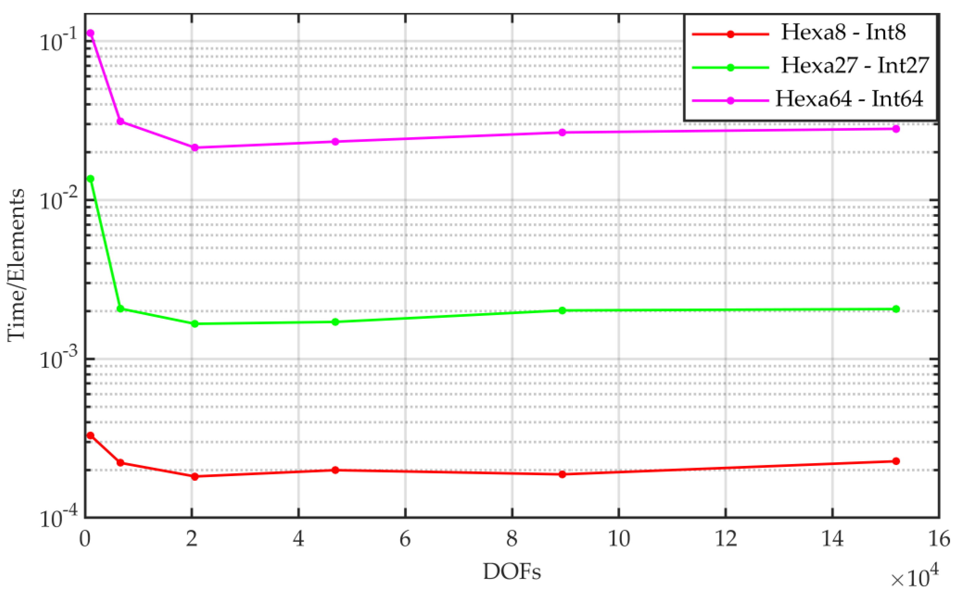
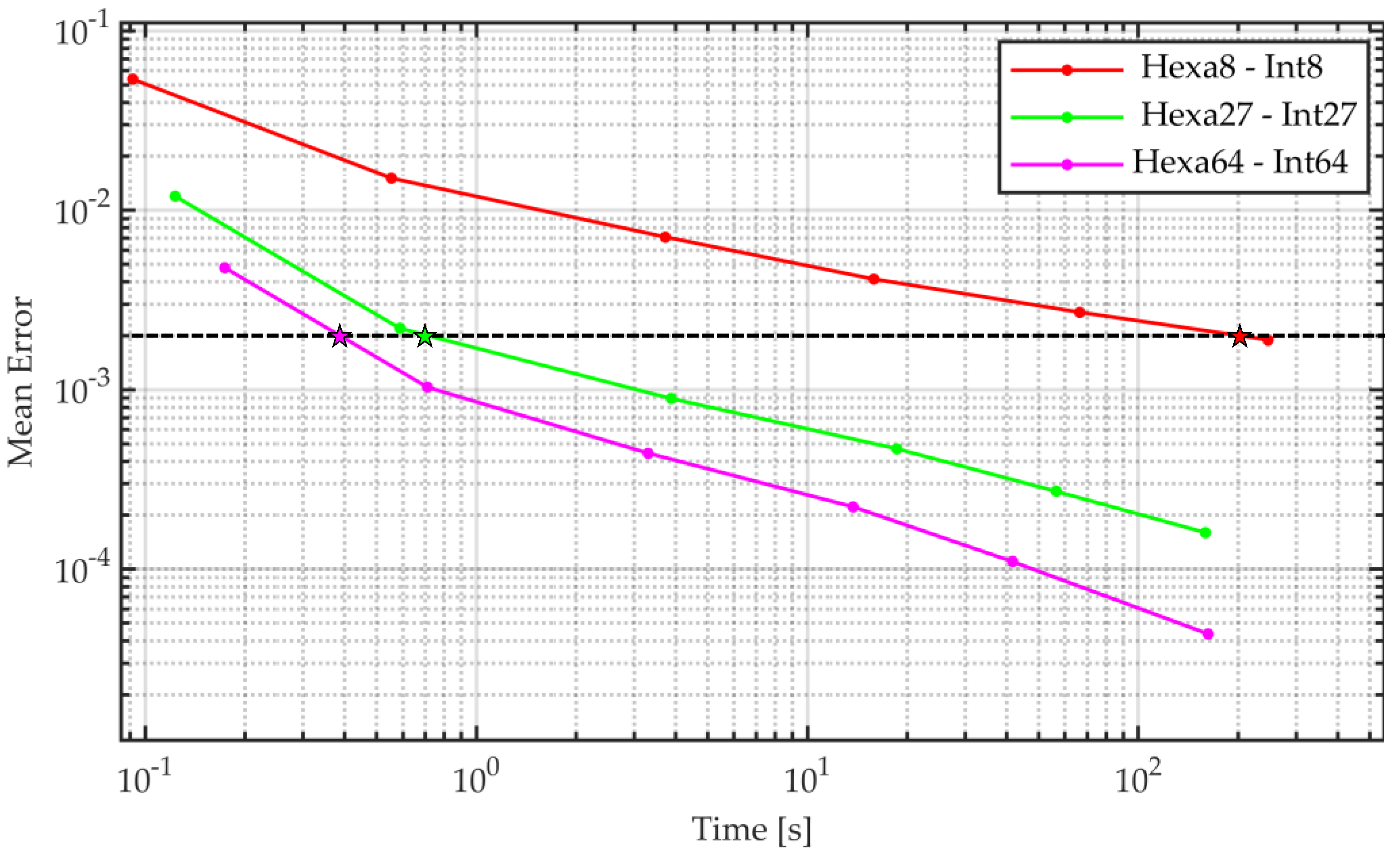
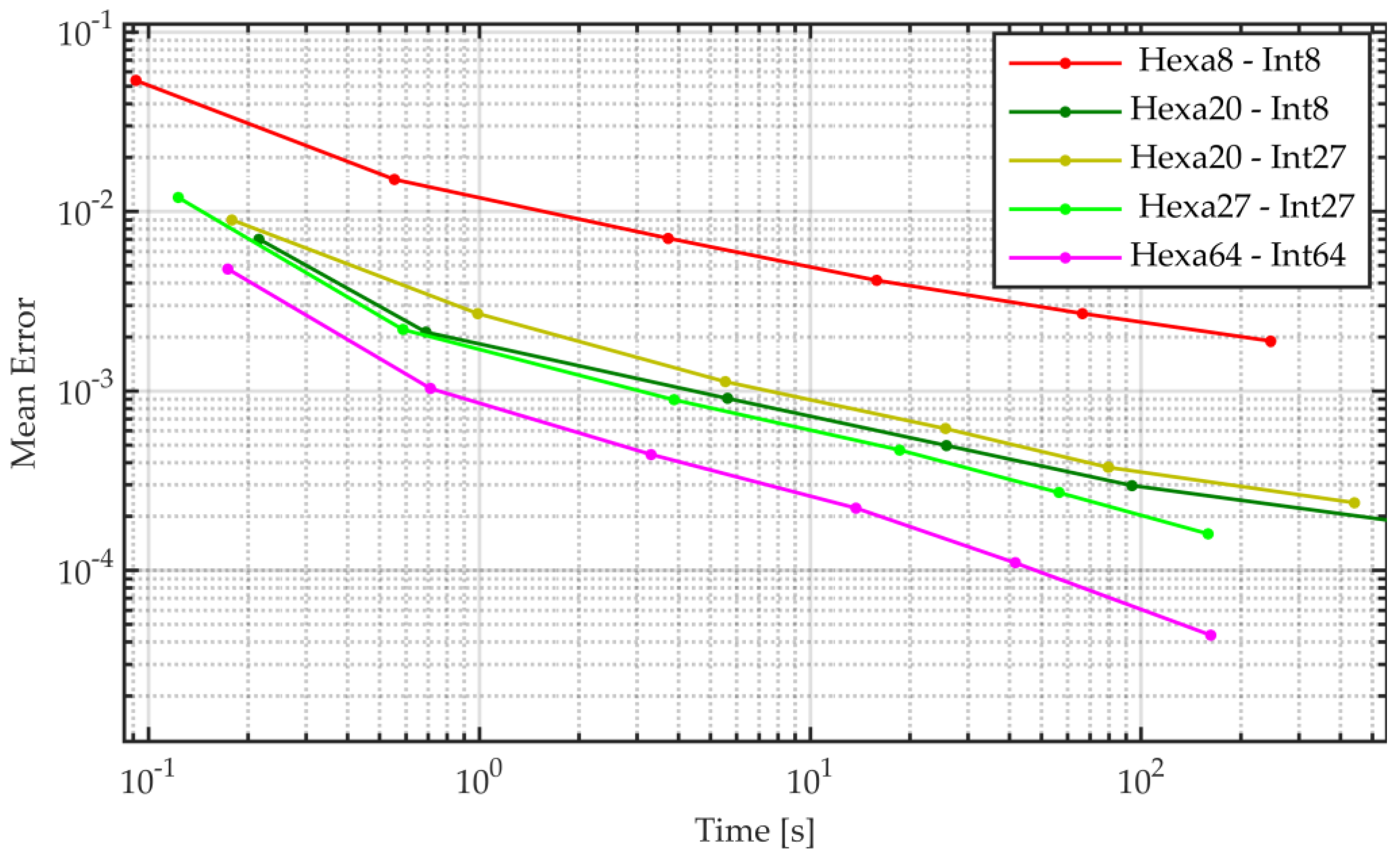
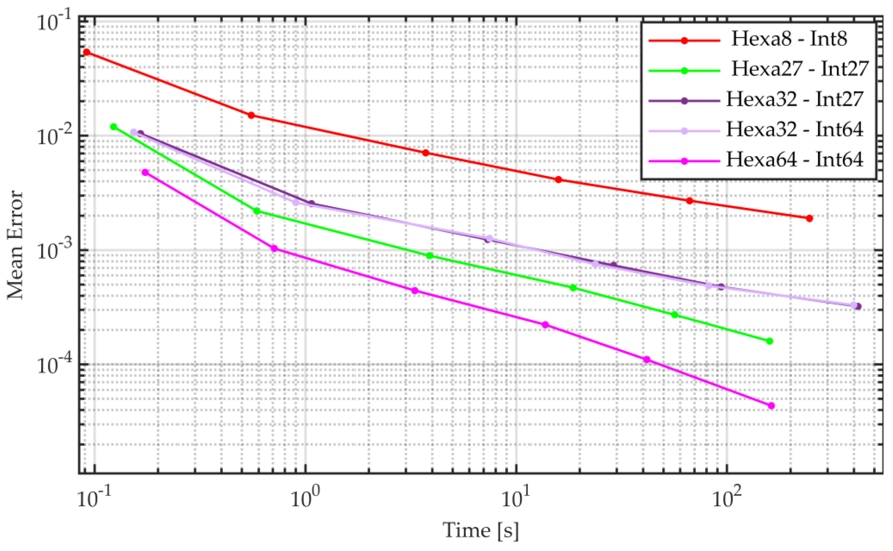
5.2. Accuracy vs. Assembly Time

This section reports on the computational efficiency of the considered FE formulations, particularly focusing on the time required by the stage of assembling the mass and the stiffness matrices (assembly time).

Figure 5 clarifies the superior performance of the higher-order formulations with respect to the linear one. The achievement of a relative accuracy of 0.2% with the linear element requires an execution time of about 9 s, while only 1.5 and 0.45 s are required for the quadratic and cubic formulations, respectively, corresponding to speed-up factors of about 6× and 20×.

The reported results may seem controversial with common sense, according to which higher-order elements are computationally more demanding.

As reported in Figure 6, the assembly time averaged by the number of elements still agrees with the expected assumptions, with the quadratic and cubic formulations featuring, respectively, nearly one and two orders of magnitude larger timings. However, the resulting formulations also provide faster convergence and demand drastically lower numbers of elements to maintain the same number of DOFs. All considered, it is reasonable that higher-order elements may provide better computational efficiency. For the assembly stage, the quadratic formulation (hexa27-int27) shows slightly better results than the cubic one (hexa64-int64). Due to their relatively bigger size, the quadratic and especially the cubic elements may become suitable for acceleration by means of GPU processing, making the computational advantages even more pronounced in favor of the higher-order formulations [79].

Figure 7 and Figure 8 depict the computational efficiency of the serendipity quadratic and cubic formulations, respectively. As expected, the quadratic serendipity formulation with reduced integration (hexa20-int8) provides the best computational efficiency, whereas both the cubic serendipity formulations (hexa32-int27) and (hexa32-int64) showed performance degradations as compared to the full-order cubic element (hexa64-int64).

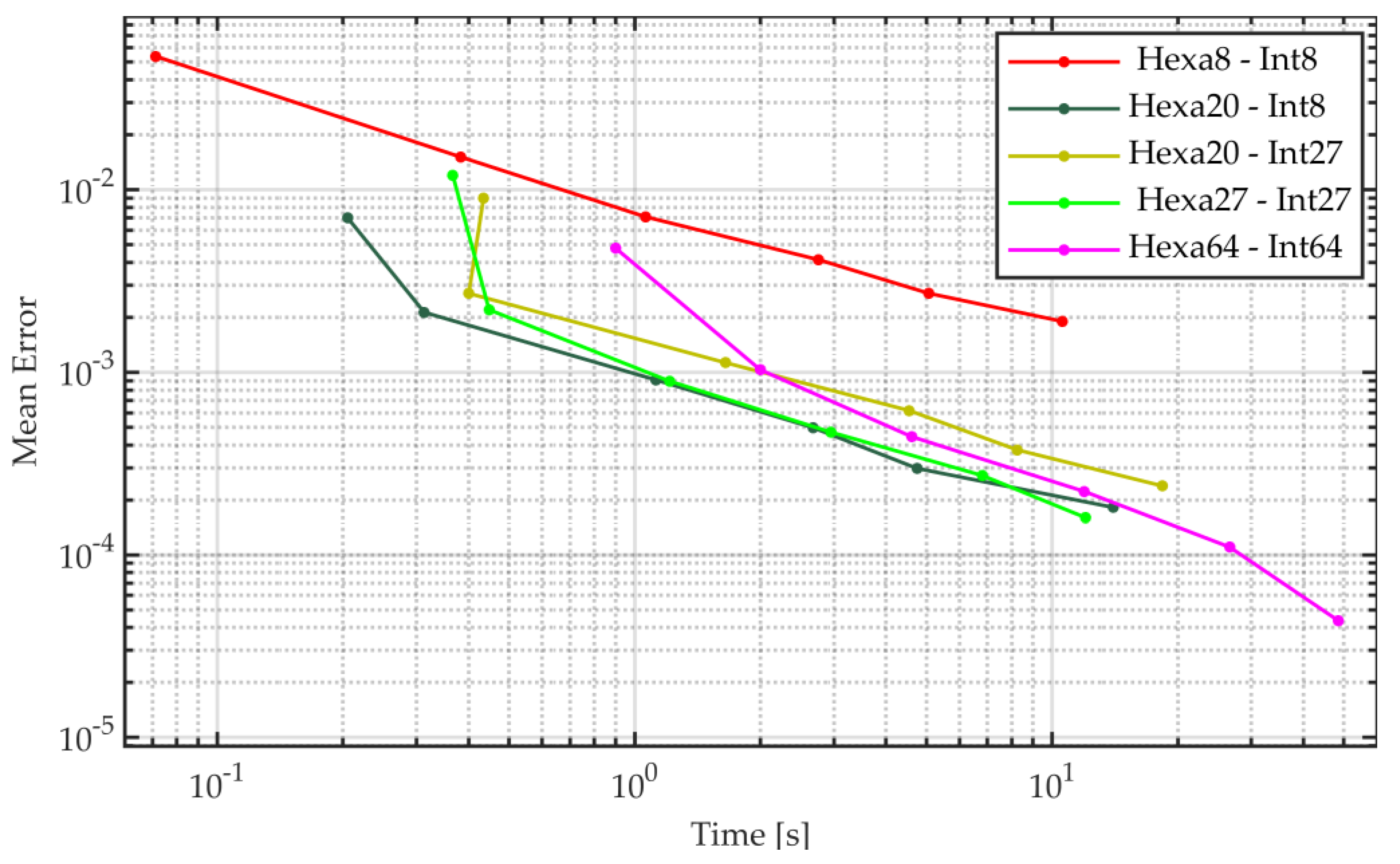
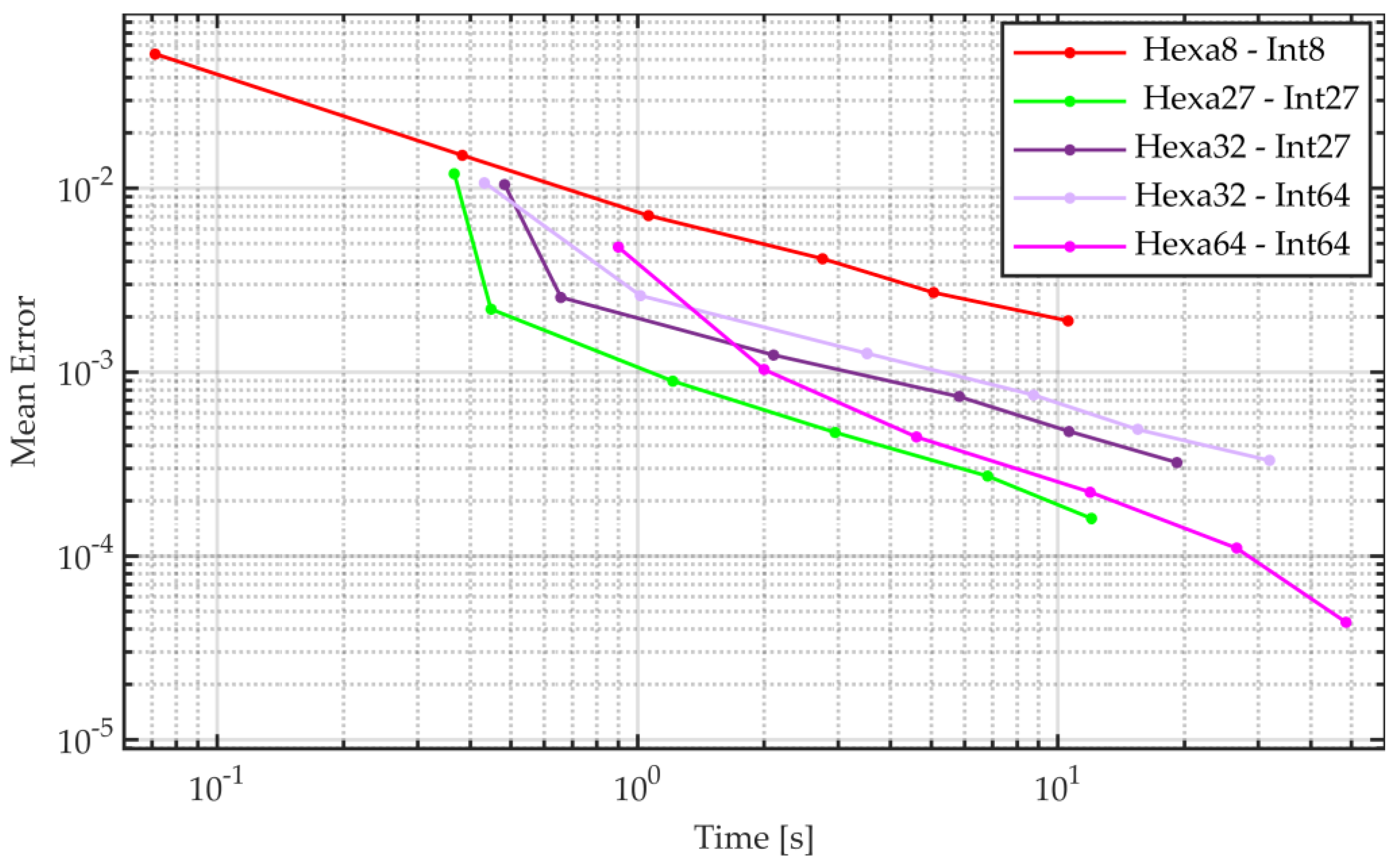
5.3. Accuracy vs. Eigenvalue Computational Time

This section further analyzes the computational and efficiency performance of the reviewed FE formulations by looking at the time required to solve the eigenvalue problem.

Similar to what was reported in the previous sub-section, higher-order elements exhibit better results. The best computational efficiency is shown in Figure 9 by the cubic elements (Hexa64-int64). For achieving an accuracy of 0.2%, the linear formulation requested the finest mesh size and took more than 200 s to perform. The quadratic and cubic meshes achieved the same accuracy, respectively, within 0.7 and 0.4 s, corresponding to speed-up factors of 286× and 500× times faster than the linear solution.

Figure 10 and Figure 11 show the computational efficiency trends of the quadratic and cubic serendipity elements. Quadratic serendipity elements (Figure 10) perform better when combined with a reduced integration scheme. It is also interesting to note that the full-order quadratic elements exhibit a convergence with a slightly larger slope, indicating that they may converge even faster for decreasing mesh sizes. In line with the results shown for the assembly stage, drastic performance degradation is appreciated for the cubic serendipity elements, making them worse than the second-order elements.

6. Conclusions

Although FEM is a mature widespread technology, the accuracy and efficiency of the obtained results are still highly influenced by user expertise. The choice of the shape functions has a strong impact on the performance as follows: the proper choice should be made to minimize the computational effort while achieving the desired level of accuracy. A wrong choice of the element type can be a source of potential issues, especially if the element does not capture accurately the simulated physics, or it may demand excessively dense meshes, which in turn leads to computational inefficiencies.

Supported by the common belief that hexahedral elements outperform other types of formulations, a systematic review of several brick formulations was performed with the aim of comparing the performances of linear, quadratic, and cubic elements, including their serendipity variants.

The reported results clearly showed that the best choice should be made according to the considered application. In applications dominated by assembly time demands, e.g., where remeshing is performed iteratively, second-order brick elements provide the best computational efficiency, with serendipity elements achieving almost the same accuracy when complemented by the reduced integration schemes. For dynamic investigations, when the time spent on the solution of the eigenvalue problems represents the bottleneck, the regular cubic formulation outperformed both linear and quadratic variants.

The reported study will be further developed by extending the performance analysis of the considered formulations in a parallel computing environment, in which the quadratic and especially the cubic elements are expected to become suitable for acceleration by means of GPU processing.

References

1. Greco, F.; Arroyo, M. High-order maximum-entropy collocation methods. Comput. Methods Appl. Mech. Eng. 2020, 367, 113115. [Google Scholar] [CrossRef]
2. Badia, S.; Codina, R.; Espinoza, H. Stability, Convergence, and Accuracy of Stabilized Finite Element Methods for the Wave Equation in Mixed Form. J. Numer. Anal. 2014, 52, 1729–1752. [Google Scholar] [CrossRef]
3. Trefethen, L.N. Accuracy, Stability and Convergence. In Finite Difference and Spectral Methods for Ordinary and Partial Differential Equations, 1st ed.; Cornell University: Ithaca, NY, USA, 1996; Chapter 4; pp. 146–188. [Google Scholar]
4. Gabard, G.; Astley, R.J.; Tahar, M.B. Stability and accuracy of finite element methods for flow acoustics: General theory and application to one-dimensional propagation. Int. J. Numer. Methods Eng. 2005, 63, 947–973. [Google Scholar] [CrossRef]
5. Willberg, C.; Duczek, S.; Vivar Perez, J.M.; Schmicker, D.; Gabbert, U. Comparison of different higher order finite element schemes for the simulation of Lamb waves. Comput. Methods Appl. Mech. Eng. 2012, 241, 246–261. [Google Scholar] [CrossRef]
6. Niiranen, J. A-Priori and a-Posteriori Error Analysis of Finite Element Methods for Plate Models. Ph.D. Thesis, Helsinki University of Technology, Espoo, Finland, 2007. [Google Scholar]
7. Kröner, A.; Kröner, H. A priori error estimates for finite element approximations of regularized level set flows in higher norms. Appl. Numer. Math. 2022, 171, 307–328. [Google Scholar] [CrossRef]
8. Irimie, S.; Bouillard, P. A residual a posteriori error estimator for the finite element solution of the Helmholtz equation. Comput. Methods Appl. Mech. Eng. 2001, 190, 4027–4042. [Google Scholar] [CrossRef]
9. Guddati, M.N.; Yue, B. Modified integration rules for reducing dispersion error in finite element methods. Comput. Methods Appl. Mech. Eng. 2004, 193, 275–287. [Google Scholar] [CrossRef]
10. Wang, Y.; Wang, J.C.D. An hp-version adaptive finite element algorithm for eigensolutions of moderately thick circular cylindrical shells via error homogenisation and higher-order interpolation. Eng. Comput. 2022, 39, 1874–1901. [Google Scholar] [CrossRef]
11. Jonckheere, S.; Bériot, H.; Dazel, O.; Desmet, W. An adaptive order finite element method for poroelastic materials described through the Biot equations. Int. J. Numer. Methods Eng. 2022, 123, 1329–1359. [Google Scholar] [CrossRef]
12. Demkowiczt, L.; Babuska, I. P interpolation error estimates for edge finite elements of variable order in two dimensions. SIAM J. Numer. Anal. 2004, 41, 1195–1208. [Google Scholar] [CrossRef]
13. Apel, T. Interpolation in h-Version Finite Element Spaces. In Encyclopedia of Computational Mechanics, Online ed.; Wiley: Chichester, MA, USA, 2004; Volume 1, pp. 67–101. [Google Scholar]
14. Jodlbauer, D.; Langer, U.; Wick, T. Parallel Matrix-Free Higher-Order Finite Element Solvers for Phase-Field Fracture Problems. Math. Comput. Appl. 2020, 25, 40. [Google Scholar] [CrossRef]
15. Drouet, G.; Hild, P. An accurate Local Average Contact (LAC) method for nonmatching meshes in 2D and 3D. Numer. Mathods 2017, 136, 467–502. [Google Scholar] [CrossRef]
16. Lin, T.; Lin, Y.; Sun, W. Error estimation of a class of quadratic immersed finite element methods for elliptic interface problems. Disc. Cont. Dyn. Syst. 2007, 7, 807–823. [Google Scholar] [CrossRef]
17. Benzley, S.; Perry, E.; Merkley, K.; Clark, B. A Comparison of All Hexagonal and All Tetrahedral Finite Element Meshes for Elastic and Elasto-plastic Analysis. In Proceedings of the 4th International Meshing Roundtable, Sandia National Laboratories, Albuquerque, NM, USA, 6 October 1995. [Google Scholar]
18. Rand, A.; Gillette, A.; Bajaj, C. Quadratic serendipity finite elements on polygons using generalized barycentric coordinates. Math. Comput. 2014, 83, 2691–2716. [Google Scholar] [CrossRef] [PubMed]
19. Liu, G.R.; Quek, S.S. The Finite Element Method. A Practical Course, 2nd ed.; Butterworth-Heinemann: Oxford, UK, 2013; p. 456. [Google Scholar]
20. Zienkiewicz, O.C.; Taylor, R.L.; Zhu, J.R. The Finite Element Method: Its Basis and Fundamentals, 7th ed.; Butterworth-Heinemann: Oxford, UK, 2013; p. 756. [Google Scholar]
21. Belytschko, T.; Fish, J. A First Course in Finite Elements, 1st ed.; Wiley: Hoboken, NJ, USA, 2007; p. 320. [Google Scholar]
22. Arnold, D.N.; Awanou, G. Finite element differential forms on cubical meshes. Math. Comput. 2014, 83, 1551–1570. [Google Scholar] [CrossRef]
23. Wang, Y. An h-version adaptive FEM for eigenproblems in system of second order ODEs: Vector Sturm-Liouville problems and free vibration of curved beams. Eng. Comput. 2020, 38, 1807–1830. [Google Scholar] [CrossRef]
24. Wang, L.; Zhong, H. A time finite element method for structural dynamics. Appl. Math. Model. 2017, 41, 445–461. [Google Scholar] [CrossRef]
25. Bathe, K.J.; Wilson, E.L. Numerical Methods in Finite Element Analysis, 1st ed.; Prentice Hall: Hoboken, NJ, USA, 1976; p. 528. [Google Scholar]
26. Bathe, K.J. Finite Element Procedures, 2nd ed.; Prentice Hall: Hoboken, NJ, USA, 2014; p. 1065. [Google Scholar]
27. Pashkevich, A.; Klimchik, A.; Chablat, D.; Wenger, P. Accuracy Improvement for Stiffness Modeling of Parallel Manipulators. In Proceedings of the CIRP Conference on Manufacturing Systems, Grenoble, France, 3–5 June 2009. [Google Scholar]
28. Tsukerman, I. A General Accuracy Criterion for Finite Element Approximation. IEEE Trans. Magn. 1998, 34, 2425–2428. [Google Scholar] [CrossRef]
29. González-Estrada, O.A.; Natarajan, S.; Ródenas, J.J.; Bordasad, S.P. Error estimation for the polygonal finite element method for smooth and singular linear elasticity. Comput. Math. Appl. 2021, 92, 109–119. [Google Scholar] [CrossRef]
30. Banz, L.; Hernández, O.; Stephan, E.P. A priori and a posteriori error estimates for ℎ𝑝-FEM for a Bingham type variational inequality of the second kind. Comput. Math. Appl. 2022, 126, 14–30. [Google Scholar] [CrossRef]
31. Cook, R.D.; Malkus, D.S.; Plhesha, M.E.; Witt, R.J. Concepts and Applications of Finite Element Analysis; John Wiley & Sons: New York, NY, USA, 2002; p. 719. [Google Scholar]
32. Hughes, T.J.R.; Evans, J.A.; Reali, A. Finite element and NURBS approximations of eigenvalue, boundary-value, and initial-value problems. Comput. Methods Appl. Mech. Eng. 2014, 272, 290–320. [Google Scholar] [CrossRef]
33. Gratsch, T.; Bathe, K.J. A posteriori error estimation techniques in practical finite element analysis. Comput. Struct. 2005, 83, 235–265. [Google Scholar] [CrossRef]
34. Babuska, I.; Rheinboldt, W.C. Error estimates for adaptive finite element computations. SIAM J. Numer. Anal. 1978, 15, 736–754. [Google Scholar] [CrossRef]
35. Zienkiewicz, O.C.; Zhu, J.Z. A Simple Error Estimator and Adaptive Procedure for practical Engineering Analysis. Int. J. Numer. Methods. Eng. 1987, 24, 337–357. [Google Scholar] [CrossRef]
36. Demkowicz, L.; Kurtz, J.; Pardo, D.; Paszynski, M.A. Computing with hp-Adaptive Finite Elements, 1st ed.; Chapman and Hall/CRC: Boca Raton, FL, USA, 2007; p. 440. [Google Scholar]
37. Demkowicz, L.; Kurtz, J.; Qiu, F. hp-adaptive finite elements for coupled multiphysics wave propagation problems. Comput. Methods. Mech. 2010, 1, 19–42. [Google Scholar]
38. Nguyen-Hoang, S.; Sohn, D.; Kim, H.-G. A new polyhedral element for the analysis of hexahedral-dominant finite element models and its application to nonlinear solid mechanics problems. Comput. Methods Appl. Mech. Eng. 2017, 324, 248–277. [Google Scholar] [CrossRef]
39. Talebi, H.; Zi, G.; Silani, M.; Samaniego, E.; Rabczuk, T. A Simple Circular Cell Method for Multilevel Finite Element Analysis. J. Appl. Math. 2012, 2012, 526846. [Google Scholar] [CrossRef]
40. Fan, Q.; Zhang, Q.; Liu, G. A Stress Analysis of a Conical Pick by Establishing a 3D ES-FEM Model and Using Experimental Measured Forces. Appl. Sci 2019, 9, 5410. [Google Scholar] [CrossRef]
41. Neto, M.A.; Amaro, A.; Roseiro, L.; Cirne, J.; Leal, R. Engineering Computation of Structures: The Finite Element Method, 1st ed.; Springer: Cham, Switzerland, 2015; p. 327. [Google Scholar]
42. Kuhn, C.; Muller, R. Exponential finite element shape functions for a phase field model of brittle fracture. In Proceedings of the XI International Conference on Computational Plasticity Fundamentals and Applications, Barcelona, Spain, 7–9 September 2011. [Google Scholar]
43. Christ, D.; Cervera, M.; Chiumenti, M. A mixed Finite Element formulation for incompressibility using linear displacement and pressure interpolations. In Monograph CIMNE, 1st ed.; CIMNE: Barcelona, Spain, 2003; pp. 1–79. [Google Scholar]
44. Felippa, C. Shear Locking in Turner Triangle. In Introduction to Finite Element Methods, 1st ed.; Aerospace Engineering Sciences Department, University of Colorado: Boulder, CO, USA, 2004; Volume 1, p. 791. [Google Scholar]
45. Visintainer, M.R.; Bittencourt, E.; Braun, A.L. A numerical investigation on contact mechanics applications using eight-node hexahedral elements with underintegration techniques. Lat. Am. J. Solids Struct. 2021, 18, 1–31. [Google Scholar] [CrossRef]
46. Li, K.P.; Cescotto, S. An 8-node brick element with mixed formulation for large deformation analyses. Comput. Methods Appl. Mech. Eng. 1997, 141, 157–204. [Google Scholar] [CrossRef]
47. Zhu, Y.Y.; Cescotto, S. Unified and mixed formulation of the 8-node hexahedral elements by assumed strain method. Comput. Methods Appl. Mech. Eng. 1997, 129, 177–209. [Google Scholar] [CrossRef]
48. Ntioudis, S. Hourglass Control in Non-Linear Finite Element Analysis, Using Hexahedral Elements. Ph.D. Thesis, University of Thessaly, Volos, Greece, 12 October 2018. [Google Scholar]
49. Liu, G.R.; Nguyen-Xuan, H.; Nguyen-Thoi, T. A variationally consistent αFEM (VCαFEM) for solution bounds and nearly exact solution to solid mechanics problems using quadrilateral elements. Int. J. Numer. Methods Eng. 2011, 85, 461–497. [Google Scholar] [CrossRef]
50. Flanagan, D.P.; Belytschko, T. A uniform strain hexadron and quadrilateral with orthogonal hourglass control. Internat. J. Numer. Methods Eng. 1981, 17, 679–706. [Google Scholar] [CrossRef]
51. Hughes, T.G.R. The Finite Element Method: Linear Static and Dynamic Finite Element Analysis, 1st ed.; Dover Publications: Mineola, NY, USA, 2000; p. 704. [Google Scholar]
52. Reese, S.; Wriggers, P. A stabilization technique to avoid hourglassing in finite elasticity. Int. J. Numer. Methods Eng. 2000, 48, 79–109. [Google Scholar] [CrossRef]
53. Araujo-Cabarcas, J.C.; Engström, C. On spurious solutions in finite element approximations of resonances in open systems. Comput. Math. Appl. 2017, 74, 2385–2402. [Google Scholar] [CrossRef]
54. Mirbagheri, Y.; Nahvi, H.; Parvizian, J.; Düster, A. Reducing spurious oscillations in discontinuous wave propagation simulation using high-order finite elements. Comput. Math. Appl. 2015, 70, 1640–1658. [Google Scholar] [CrossRef]
55. Ko, Y.; Bathe, K.-J. A new 8-node element for analysis of three-dimensional solids. Comput. Struct. 2018, 202, 85–104. [Google Scholar]
56. Karpik, A.; Cosco, F.; Mundo, D. On the Profitability of Higher Order FE Formulations for Structural Dynamics. In Proceedings of the IFToMM, Naples, Italy, 7–9 September 2022. [Google Scholar]
57. Danielson, K.T.; Adley, M.D.; Williams, T.N. Second-order finite elements for Hex-Dominant explicit methods in nonlinear solid dynamics. Finite Elements Anal. Des. 2016, 119, 63–77. [Google Scholar] [CrossRef]
58. Liu, Y. Effects of Mesh Density on Finite Element Analysis. SAE Tech. Pap. 2013, 1375, 1–8. [Google Scholar]
59. Rachowicz, W.; Pardob, D.; Demkowicz, L. Fully automatic hp-adaptivity in three dimensions. Comput. Methods Appl. Mech. Eng. 2006, 195, 4816–4842. [Google Scholar] [CrossRef]
60. Song, S.; Braun, M.; Wiegard, B.; Herrnring, H.; Ehlers, S. Combining H-Adaptivity with the Element Splitting Method for Crack Simulation in Large Structures. Materials 2022, 15, 240. [Google Scholar] [CrossRef] [PubMed]
61. Babuska, I.; Szabo, B.A.; Katz, I.N. The p-version of the finite element method. SIAM J. Numer. Anal. 1981, 18, 515–545. [Google Scholar] [CrossRef]
62. Eisenträger, S.; Atroshchenko, E.; Makvandi, R. On the condition number of high order finite element methods: Influence of p-refinement and mesh distortion. Comput. Math. Appl. 2020, 80, 2289–2339. [Google Scholar] [CrossRef]
63. López Machado, N.A.; Vielma Pérez, J.C.; López Machado, L.J. An 8-Nodes 3D Hexahedral Finite Element and an 1D 2-Nodes Structural Element for Timoshenko Beams, Both Based on Hermitian Intepolation, in Linear Range. Mathematics 2022, 10, 836. [Google Scholar] [CrossRef]
64. Babuska, I.; Szabo, B. On the Rates of Convergence of the Finite Element Method. Int. J. Numer. Meth. Eng. 1982, 18, 323–341. [Google Scholar] [CrossRef]
65. Babuska, I. The p- and hp-Versions of the Finite Element Method: The State of the Art, Finite Elements. In Book Finite Elements: Theory and Applications, 1st ed.; Springer: New York, NY, USA, 2011; Volume 1, p. 312. [Google Scholar]
66. Lo, S.H. Finite Element Mesh Generation, 1st ed.; CRC Press: Boca Raton, FL, USA, 2015; p. 672. [Google Scholar]
67. Zhoul, P.L.; Cen, S.; Huang, J.B.; Li, C.F.; Zhang, Q. An unsymmetric 8-node hexahedral element with high distortion tolerance. Int. J. Numer. Meth. Eng. 2016, 109, 1130–1158. [Google Scholar]
68. Shang, Y.; Li, C.F.; Jia, K.Y. Jia 8-node hexahedral unsymmetric element with rotation degrees of freedom for modified couple stress elasticity. Int. J. Numer. Methods Eng. 2020, 121, 2683–2700. [Google Scholar] [CrossRef]
69. Parrish, M.; Borden, M.; Staten, M.; Benzley, S. A Selective Approach to Conformal Refinement of Unstructured Hexahedral Finite Element Meshes. In Book Proceedings of the 16th International Meshing Roundtable, 1st ed.; Springer: Washington, DC, USA, 2014; Volume 1, pp. 251–268. [Google Scholar]
70. Schneider, T.; Hu, Y.; Gao, X.; Dumas, J.; Zorin, D.; Panozzo, D. A large-scale comparison of tetrahedral and hexahedral elements for solving elliptic PDEs with the finite element method. ACM Trans. Graph. 2022, 41, 1–14. [Google Scholar] [CrossRef]
71. Mohsen, A.; Moslemi, H.; Seddighian, M.R. An Improved Nodal Ordering for Reducing the Bandwidth in FEM. J. Serbian Soc. Comput. Mech. 2018, 12, 126–143. [Google Scholar] [CrossRef]
72. Zeng, K. Automatic Generation of Compact Models for the Efficient Calculation of MEMS Structures, 1st ed.; Cuvillier Verlag: Göttingen, Germany, 2005; p. 150. [Google Scholar]
73. Zhang, J.; Kikuchi, F. Interpolation error estimates of a modified 8- node serendipity finite element. Numer. Math. 2000, 85, 503–524. [Google Scholar] [CrossRef]
74. Arnold, D.N.; Awanou, G. The serendipity family of finite elements. Found. Comput. Math. 2011, 11, 337–344. [Google Scholar] [CrossRef]
75. Browning, R.S. A Second-Order 19-Node Pyramid Finite Element Suitable for Lumped Mass Explicit Dynamic Methods in Nonlinear Solid Mechanics. Ph.D. Thesis, University of Alabama at Birmingham, Birmingham, AL, USA, September 2020. [Google Scholar]
76. Lee, N.; Bathe, K.-J. Effects of element distortions on the performance of isoparametric elements. Int. J. Numer. Methods Eng. 1993, 36, 3553–3576. [Google Scholar] [CrossRef]
77. Liu, G.R.; Nguyen-Xuan, H.; Nguyen-Thoi, T. A theoretical study on the smoothed FEM (S-FEM) models: Properties, accuracy and convergence rates. Int. J. Numer. Methods Eng. 2010, 84, 1222–1256. [Google Scholar] [CrossRef]
78. Kressner, D. The Krylov-Schur Algorithm. In Numerical Methods for General and Structured Eigenvalue Problem, 1st ed.; Springer: Berlin/Heidelberg, Germany, 2005; Volume 1, pp. 113–130. [Google Scholar]
79. Cosco, F.; Greco, F.; Desmet, W.; Mundo, D. GPU accelerated initialization of local maximum-entropy meshfree methods for vibrational and acoustic problems. Comput. Methods Appl. Mech. Eng. 2020, 36, 113089. [Google Scholar] [CrossRef]
Figure 1. 3D clamped cube model (a) and the corresponding FE cubic mesh (b).
Machines 11 00326 g001
Figure 2. Convergence analysis of the full−order FE formulations as a function of the number of DOFs.
Machines 11 00326 g002
Figure 3. Convergence analysis of three FE formulations (quadratic, serendipity 20−nodes, and serendipity 20−nodes with reduced integration) as a function of the number of DOFs in comparison with linear and cubic full elements.
Machines 11 00326 g003
Figure 4. Convergence analysis of three FE formulations (cubic, serendipity 32−nodes, and serendipity 32−nodes with reduced integration) as a function of the number of DOFs in comparison with linear and quadratic full elements.
Machines 11 00326 g004
Figure 5. Convergence analysis of full−order linear, quadratic, and cubic FE formulations as a function of the assembly time.
Machines 11 00326 g005
Figure 6. Average (per element) assembly time of the full−order linear, quadratic, and cubic FE formulations as a function of the number of DOFs.
Machines 11 00326 g006
Figure 7. Convergence analysis of serendipity quadratic FE formulations as a function of the assembly time in comparison with full−order elements.
Machines 11 00326 g007
Figure 8. Convergence analysis of serendipity cubic FE formulations as a function of the assembly time in comparison with full−order elements.
Machines 11 00326 g008
Figure 9. Convergence analysis of full−order linear, quadratic, and cubic FE formulations as a function of the time for eigenvalue computations.
Machines 11 00326 g009
Figure 10. Convergence analysis of quadratic serendipity FE formulations as a function of the time for eigenvalue computation in comparison with full−order elements.
Machines 11 00326 g010
Figure 11. Convergence analysis of cubic serendipity FE formulations as a function of the time for eigenvalue computation in comparison with full−order elements.
Machines 11 00326 g011