Q-Learning with the Variable Box Method: A Case Study to Land a Solid Rocket

Abstract

Some critical tasks require refined actions near the target, for instance, steering a car in a crowded parking lot or landing a rocket. These tasks are critical because failure to comply with the constraints near the target may lead to a fatal (unrecoverable) condition. Thus, a higher resolution action is required near the target to increase maneuvering precision. Moreover, completing the task becomes more challenging if the environment changes or is uncertain. Therefore, novel approaches have been proposed for these problems. In particular, reinforcement learning schemes such as Q-learning have been suggested to learn from scratch, subject to exploring action–state causal relationships aimed at action decisions that lead to an increase in the reward. Q-learning refines iterative action inputs by exploring state spaces that maximize the reward. However, reducing the (constant) resolution box needed for critical tasks increases the computational load, which may lead to the tantamount curse of the dimensionality problem. This paper proposes a variable box method to maintain a low number of boxes but reduce its resolution only near the target to increase action resolution as needed. The proposal is applied to a critical task such as landing a solid rocket, whose dynamics are highly nonlinear, underactuated, non-affine, and subject to environmental disturbances. Simulations show successful landing without leading to a curse of dimensionality, typical of the classical (constant box) Q-learning scheme.

1. Introduction

Space launches have improved autonomous landing technology for reusable spacecraft in the last few years. These aim to recover the rocket’s main booster for analysis and to retrofit, saving about 60% of total mission costs [1]. Why does it take 60 years of rocket technology development to achieve landing technology? We need to revise this briefly. First, the physics involved in a rocket landing is difficult to command; this stems from the fact that descending a vertical longitudinal rocket’s dynamics are highly nonlinear, underactuated, non-affine, and subject to environmental disturbances. This critical task requires extreme maneuverability when using thrust vector control (TVC). Furthermore, unlike the fixed nozzle configuration that commands two controllers (variable thrust and surface control), non-affine underactuation arises when using TVC because it implements one control (constant thrust with a variable nozzle placed at the rocket’s bottom end, controlling it within a small angle range). Second, TVC is used because the low approaching velocities make the surface control input irrelevant, exacerbating maneuvering toward the landing spot [2,3]. Over the years, model-based optimization schemes subject to constraints have been addressed. However, due to changing environmental conditions, the lack of exact knowledge jeopardizes the implementation of conservative model-based approaches. In these circumstances, Machine Learning (ML) tools, such as Reinforcement Learning (RL), have materialized as an alternative to learning the actions required to produce the desired trajectories.

RL algorithms exploit the reward evaluation to optimize a value function through the Bellman Equation that governs the learning process under an optimal policy. RL has solved many problems, such as automatic translation, image recognition, medical diagnosis, and text and speech recognition, to name a few. However, further algorithmic improvement is needed for physical systems due to RL iterates. Thus, critical tasks such as landing a rocket may lead to fatal failure (where the system cannot recover operation) for certain iterations. For example, RL has been used for image classification to identify landing spots for aerospace missions [4,5,6], including deep RL [7]; however, there are no studies for landing dynamical rockets.

Q-learning is a salient scheme of RL algorithms that has proven successful in uncertain dynamical systems (see Appendix A). It associates a discrete state with a discrete box corresponding to a discrete action that eventually leads to the optimal outcome after exploring the whole state space; such discretizations handle advantageous uncertainties. Classical Q-learning relies on the box method, which assigns boxes of a constant resolution (CR) corresponding to a discretized state. When a better input resolution is required, the conventional solution is to increase the number of boxes, which may lead to the curse of dimensionality [8]. Moreover, for goal-oriented tasks, the Q-algorithm’s learning architecture allows for the modification of the resolution of the boxes as the system state approaches the goal state. Thus, we aim to use a low number of boxes to maintain the low state-space dimension and reduce only the box size near the goal, avoiding the curse of dimensionality.

This paper proposes a box method with a variable resolution (VR) to increase the learning resolution where needed without increasing the computational costs or the resolution for each state variable. The VR method is applied to the Q-learning algorithm to maneuver the landing of a rocket. Representative dynamic simulations using the complex solid rocket dynamics using the real parameters of a NASA rocket are presented. It is shown that the learned policy (controls) produces admissible trajectories that comply with this critical task, even when the rocket is subject to disturbances.

This paper is organized as follows. The problem statement is presented in Section 2, followed by the proposed variable box method. Then, a brief revision of RL algorithms is given in Section 3. Section 4 introduces the TVC rocket dynamics and the simulation results are shown. Finally, the conclusions are given in Section 5.

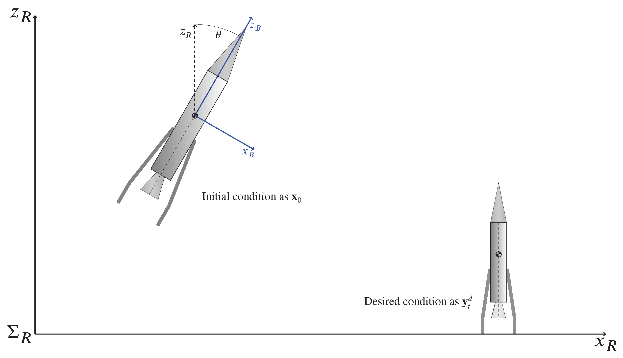
2. Problem Statement

We consider the following nonlinear, non-affine, underactuated, disturbed, and state-constrained system in the continuous state-space form given by

$$\begin{array}{cc}\hfill \dot{\mathbf{x}}& =\mathbf{f}(\mathbf{x},t)+\mathbf{g}(\mathbf{x},u,t)+\eta \left(t\right)\hfill \end{array}$$

(1)

$$\begin{array}{cc}\hfill \mathbf{y}& =\mathbf{h}\left(\mathbf{x}\right)=\mathbf{x}\hfill \end{array}$$

(2)

where $\mathbf{x},\mathbf{y}\in {\Re }^n$ are the vector state and system output, respectively, $\mathbf{f}(\mathbf{x},t)$ is the flow of the nonlinear ODE (1), $\mathbf{g}(\mathbf{x},u,t)$ is the input matrix, and $\eta \left(t\right)$ is a Liptchitz disturbance. Let the Euler method be used to obtain the following difference equation of (1) and (2),

$$\begin{array}{cc}\hfill {\mathbf{x}}_{t+1}& ={\mathbf{x}}_t+h\left[\mathbf{f}\left({\mathbf{x}}_t\right)+\mathbf{g}({\mathbf{x}}_t,u_t)+{\eta }_t\right]\hfill \end{array}$$

(3)

$$\begin{array}{cc}\hfill {\mathbf{y}}_t& ={\mathbf{x}}_t\Rightarrow {\mathbf{y}}_{t+1}={\mathbf{x}}_{t+1}\hfill \end{array}$$

(4)

where $h>0$ is the step size and ${\mathbf{y}}_t$ corresponds to the output at the t time step. Note that Systems (1) and (2), or (3) and (4), are:

1.

nonlinear (superposition theorem does not apply);

2.

underactuated (there exist more degrees of freedom than control inputs);

3.

non-affine in the control input u (since $\mathbf{g}$ cannot be written as $\mathbf{g}=\overline{\mathbf{g}}u$ for a given $\overline{\mathbf{g}}$ input matrix).

Since 1–3 account for a complex system and assuming that the task is complex for traditional control techniques, a Q-algorithm is a feasible solution using a variable resolution box method to refine the state space that allows learning from scratch, avoiding increasing the computational load. Then, assuming full access to the output vector ${\mathbf{y}}_t$ of system (3) and (4), the problem statement is how to apply the Q-Algorithm using a variable box method to produce a set of admissible trajectories with a feasible (without incurring the curse of dimensionality) iterative learning policy $u_t$ that eventually converges to its optimal $u_t^{\ast }={\pi }_{\ast }$ that maximizes a reward policy.

3. Box Methods in RL algorithms

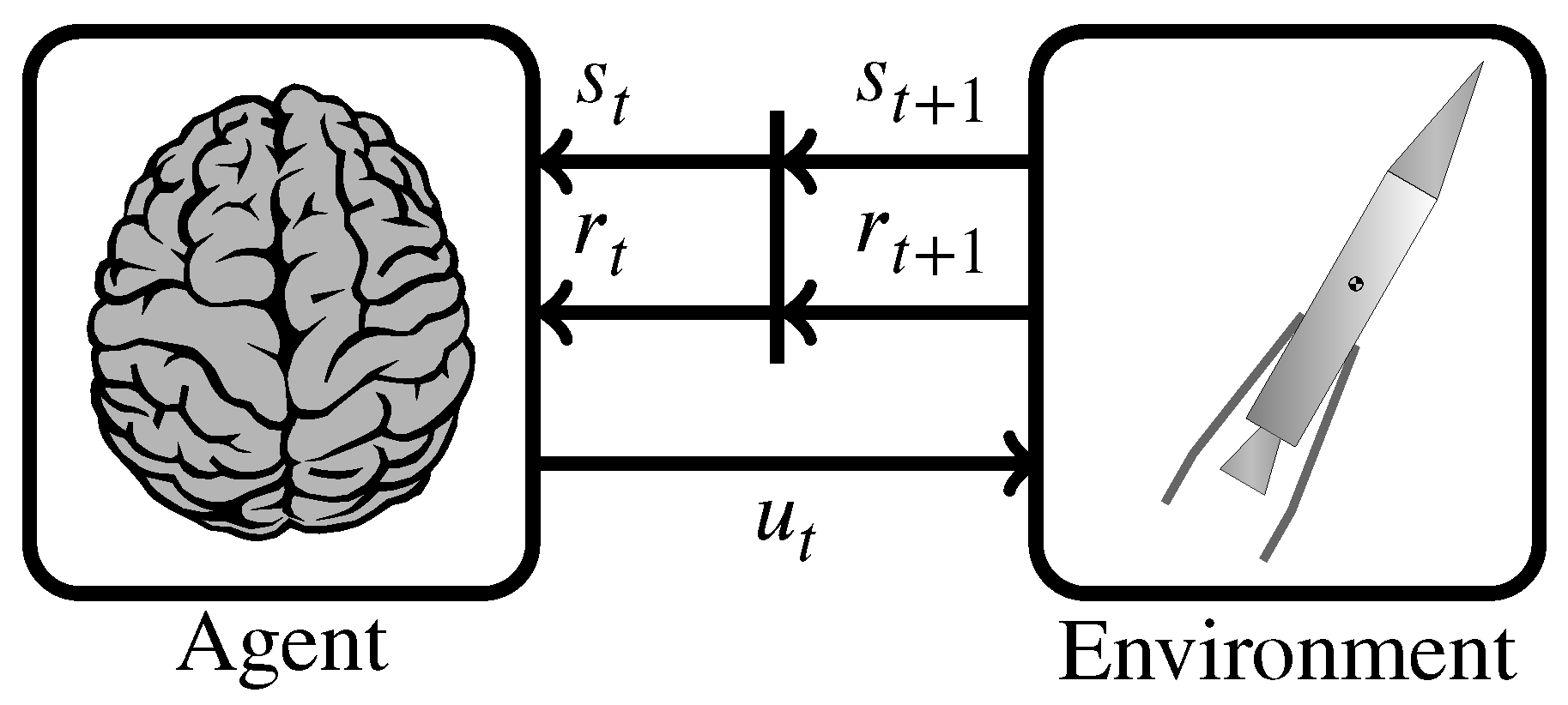
3.1. Brief Background of Reinforcement Learning

Unlike supervised or unsupervised learning, reinforcement learning is characterized as the learning process carried out from scratch, taking into account environmental information and reward assignment, typically using a Markov Decision Process (MDP) [9]. As a result, undesirable actions and states are allowed throughout the learning process. Moreover, RL avoids them in subsequent trials to improve learning. The RL idea is that the agent applies action $u_t$ to the environment, consequently producing a measurable state $s_t$ at time t, which is evaluated by a reward policy, see Figure 1. The agent’s goal is to learn the set of actions that optimizes a value cost function $V\left(s_t\right)$ throughout a long-term reward process $r_{t+1}$, which at $t+1$, leads to complying with the reward policy until $s_{t+1}$ reaches the (desired) goal state $s_{t+1}^d$. The optimization process minimizes $V\left(s_t\right)$ by assigning a value to each state, followed by a policy $\pi \left(s_t\right)$ that defines the agent’s behavior. Thus, the agent learns the behavior that leads to an optimal policy ${\pi }_{\ast }\left(s_t\right)$, and, therefore, to optimal states of an optimal value function $V_{\ast }\left(s_t\right)$. The optimization problem is solved using Dynamic Programming (DP) to satisfy the fundamental Bellman Equation.

3.2. Classical Box Method

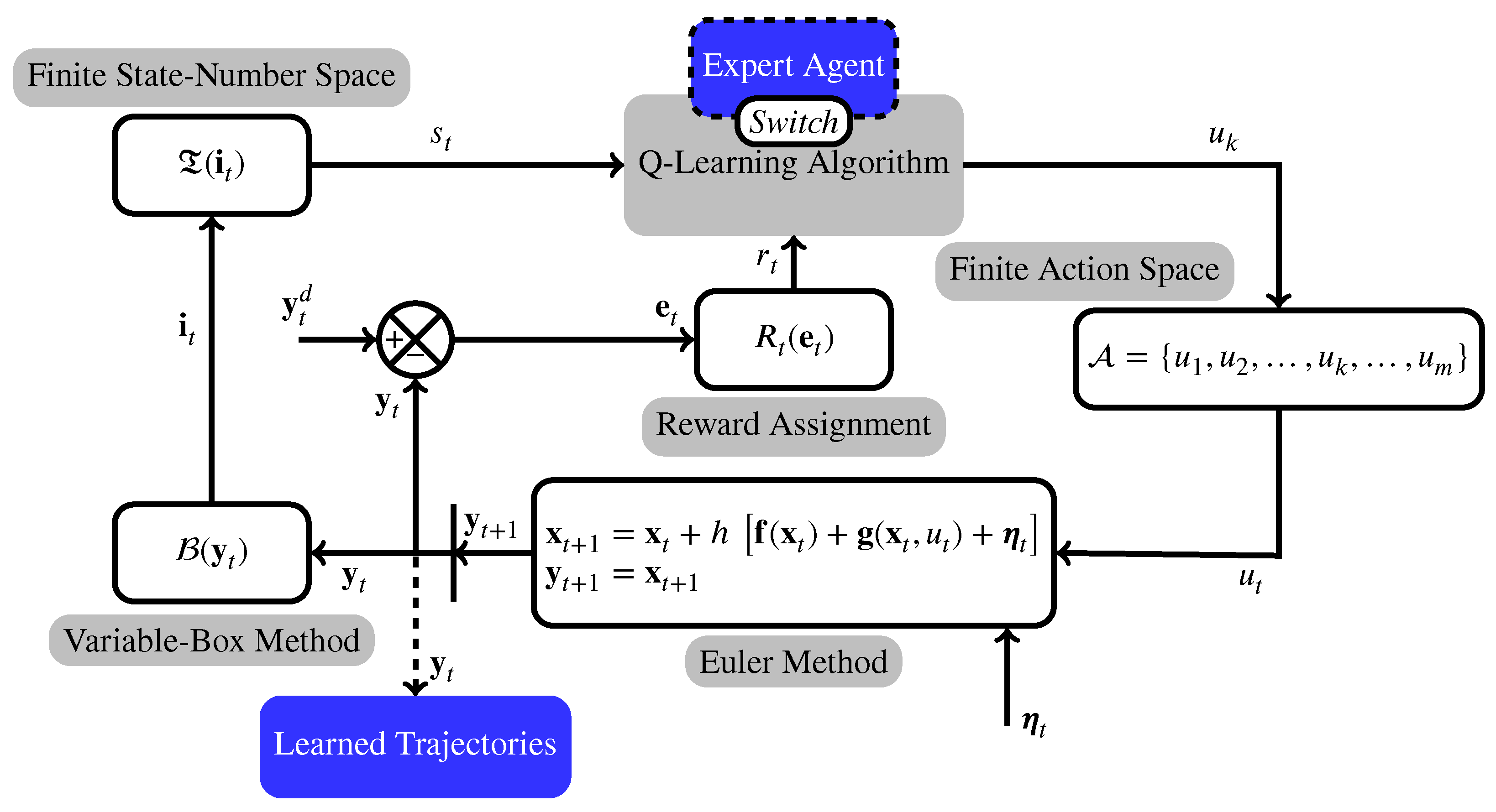
Q-learning encloses continuous state and action values into finite sets by indexing intervals into so-called boxes [10]. The classical boxing method, called the box method, uses two user parameters, the set of finite fence limits and the constant resolution $ϵ=b_{up}-b_{lw}$, which determine the size of each box based on its upper $b_{up}$ and lower $b_{lw}$ limits. Then, the i-th element of the output vector ${\mathbf{y}}_t$ is divided into $n_i$ boxes of a constant resolution $ϵ$, where t is the time step and ${\mathbf{i}}_t\in {\mathbb{N}}^N$ is the index vector. There arise N-elements of ${\mathbf{y}}_t$ as components of a new set $\mathcal{B}(·)$, where $\mathcal{B}(·)$ maps the state space to index the vector space ${\mathbf{y}}_t\mapsto {\mathbf{i}}_t$. In this way, one has the following two spaces:

-

Finite State-Number Space. Let ${\mathbf{i}}_t$ be the index vector of the finite state-number space $\mathcal{S}$ for $dim\left(\mathcal{S}\right)={\prod }_{i=1}^N(n_i+1)$, whose elements are the state numbers $s_t$ codified by ${\mathbf{i}}_t$’s elements. Then, $\mathcal{S}$ models a vector of the integer numbers’ range $[0,dim(\mathcal{S})-1]$ as elements of a tensor $\mathfrak{T}$ of N-axes, coding the state number $s_t$ into $\mathfrak{T}$ to finally relate the indexed output vector ${\mathbf{y}}_t$ to ${\mathbf{i}}_t$ and then to $s_t=\mathfrak{T}\left({\mathbf{i}}_t\right):{\mathbf{i}}_t=\mathcal{B}\left({\mathbf{y}}_t\right)$.

-

Finite Action Space. Aiming at obtaining a finite action space $\mathcal{A}=\{u_1,u_2,\dots ,u_k,\dots ,$$u_m\}$ for the bounded action (control) variable $u\in [u_{lw},u_{up}]$ represented by m-boxes of $ϵ>0$ width each, then $dim\left(\mathcal{A}\right)=m$. Each element $u_k$ is indexed by the m-th action agent from an arbitrary policy. Note that a high number of u values is suggested to enable more state-number explorations. However, this may lead to an unfeasible explosion of dimensions, or the curse of dimensionality.

In recent years, research has focused on improving learning algorithms such as deep Q-learning or actor–critic, rather than the box method, which is fundamental for many of these algorithms.

Limitations of the Classical Box Method. Methods have been proposed to deal with one of the main drawbacks of the classical box method: tuning $ϵ$ without leading to an unfeasible explosion of dimensions. Several variable boxing methods have been proposed. Ref. [11] proposes an interpolation approach using a coarse grid for the learning process and then increases the accuracy with Kuhn Triangulation around the interested regions. In [12], feudal reinforcement learning is proposed by dividing the state space into regions, where each is iterative-divided to reduce state-space searching using the manager concept, similar to the demons in neuron-like adaptive elements [13]. Ref. [14] introduced an adaptive resolution boxes approach by approximating the value function using interpolation and tree structures to refine the grid, similar to [15], using kd-trees to identify attractive state-space regions. Recently, a fuzzy action assignment method has been proposed to generate continuous control based on an optimal trained Q-table [16]. In these approaches, the resolution is adaptive online because the goal box is unknown, as in a chess game. However, there are applications where the goal is known a priori, allowing an offline variable box resolution.

3.3. The Proposed Variable Box Method

Let the $i_b$ box be variable with a resolution ${ϵ}_i$ given by

$$\begin{array}{c}\hfill {ϵ}_i=\left\{\begin{array}{cc}\hfill & {ϵ}_{i_b-1}+\frac{1}{2}{ϵ}_{gb}M\left(\right|\mathsf{\Delta }{i}_b\left|\right)\mathrm{if}\mathsf{\Delta }{i}_b>0\hfill \\ \hfill & {ϵ}_{i_b+1}+\frac{1}{2}{ϵ}_{gb}M\left(\right|\mathsf{\Delta }{i}_b\left|\right)\mathrm{if}\mathsf{\Delta }{i}_b<0\hfill \\ \hfill & {ϵ}_{gb} \mathrm{otherwise}\hfill \end{array}\right.\end{array}$$

(5)

where $|\mathsf{\Delta }{i}_b|=|i_b-i_{gb}|$, with $i_b$ the current box index and $i_{gb}$ the goal-box index. The scalar function $M\left(\right|\mathsf{\Delta }{i}_b\left|\right)\in {\mathcal{C}}^2$ is monotonous away from the origin $M\left(0\right)=0$ such that it increases (decreases) the accuracy in the vicinity of larger (smaller) distances to the goal-box resolution ${ϵ}_{gb}$. As an example of function $M\left(\right|\mathsf{\Delta }{i}_b\left|\right)$, the discrete Fibonacci Serie$\{1,1,2,3,5,\dots \}$ can be considered. The proposed algorithm for the variable box method is shown in Algorithm 1. The box resolution ${ϵ}_i$ yields:

a.

a faster reaction for larger errors;

b.

a constant box dimension; the remaining boxes are enlarged (shrank) when ${ϵ}_{i_b-1}$ is reduced (expanded), like an accordion of a fixed length;

c.

continuous action-taken history and influence [14], with smooth transitions between state numbers.

Note that for each i-th element of the output vector, $y_i\in {\mathbf{y}}_t$, there exists a goal box with an index box $i_{gb}$ and a resolution ${ϵ}_{gb}$ defined by prior knowledge of the desired state-variable value $y_i^d\in [y_{i,lw},y_{i,up}]$; each box resolution can be increased (or decreased) according to the proximity of the goal box. Additionally, ${ϵ}_{i_b}$ should be truncated to ${ϵ}_s$ for safety resolution to ensure sufficient accuracy in edged boxes; otherwise, many state vectors would be assigned the same state number. Finally, note that the classical box method is a particular case of our proposed variable box method since it is included in the third condition in (5).

Algorithm 1: The proposed variable box method enables higher resolution near the goal but lower resolution away from it to avoid exploiting dimensionality

3.4. How to Deal with the Curse of Dimensionality

A comparative grid example of the classical box and variable box methods is shown in Figure 2, considering two state variables with $y_{i,lw}=-1$ and $y_{i,up}=1$. Figure 2a uses a constant resolution ${ϵ}_i=1\times {10}^{-2}$, whereas the variable box method considers ${ϵ}_{gb}=1\times {10}^{-2}$ and ${ϵ}_s=0.1$. Note that both methods have the same box resolution and accuracy around the goal box. This way, finer action is taken with a greater reward when it is near the goal.

Otherwise, the variable box method reduces the curse of dimensionality in a Q-learning implementation using only 14.4% of boxes to render similar results to the classical box method without changing their attributes around the interested region.

3.5. Reward Assignment

A critical element of RL algorithms is the design of the reward policy because it codifies the policy that leads to the learning goal [17]. In this work, the reward is defined as an evaluation function $R_t\left({\mathbf{e}}_t\right)$ that evaluates the error of the goal of the current agent. Thus, instead of increasing the reward, which may lead to an aggressive action, we propose to increase the box resolution when needed by using the variable box method for the same reward policy to guarantee the learning goal.

The following section describes a case study showing how the proposed variable box method with Q-learning can successfully land a complex plant, as depicted in Figure 3.

4. A Case Study: Rocket Landing

The proposed variable box method is synthesized to learn the descent trajectories of a solid rocket driven by TVC using the Q-learning algorithm. First, a brief description of rocket dynamics is given, followed by the concise Lagrangian model. Then, the comparative simulation results of the classical box and variable box methods are presented.

4.1. Dynamical Model

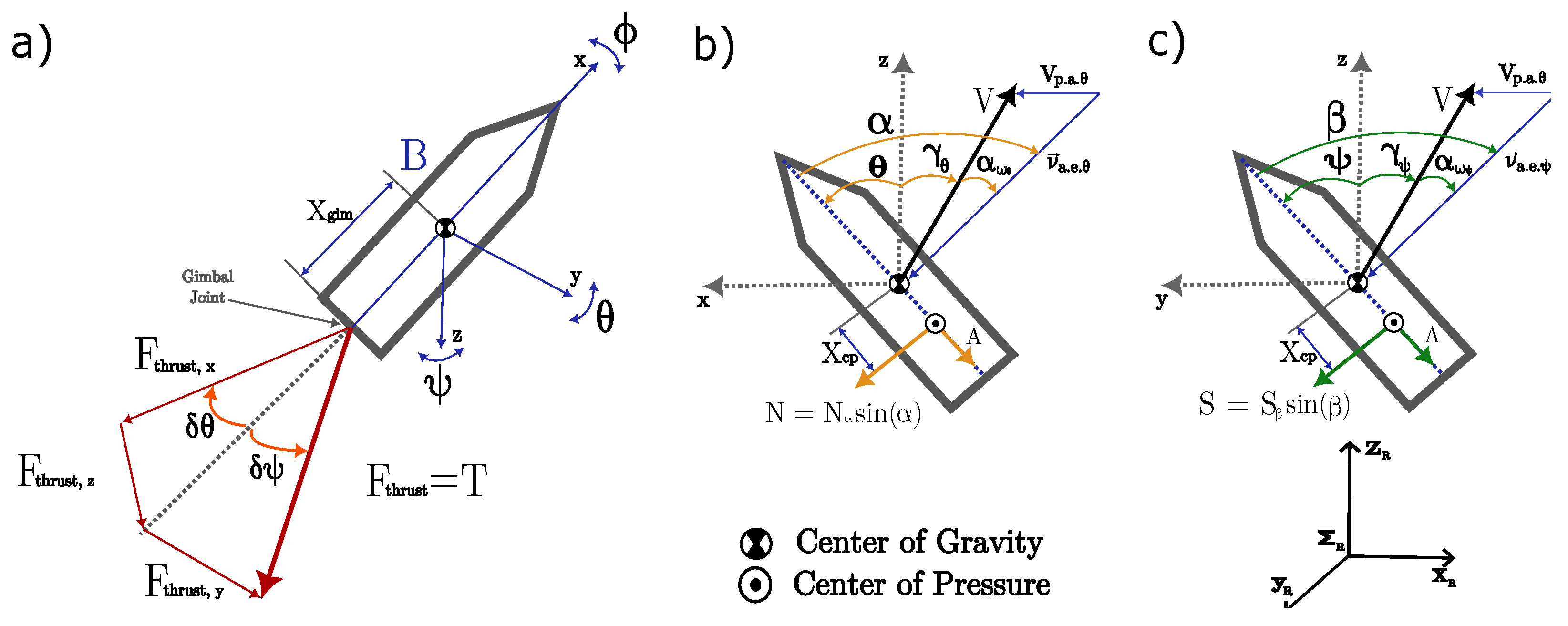
4.1.1. Translational Dynamics

Applying the second law of Newton, the forces acting on the rocket are defined as

$$\mathbf{a}=\frac{1}{m_r}\mathbf{F}=\frac{1}{m_r}[T_{ECI}^B({\mathbf{F}}_{aer}+{\mathbf{F}}_{thrust})+{\mathbf{F}}_g]$$

(6)

where $m_r$ is the rocket mass, ${\mathbf{F}}_{aer}$ are the aerodynamic forces, ${\mathbf{F}}_{thrust}$ is the thrust force, and ${\mathbf{F}}_g$ is the gravity force, with $T_R^B=R(x,\varphi )R(y,\theta )R(z,\psi )$ the rotation matrix between the reference frames B and R, see Figure 4a. Note that the thrust and aerodynamic forces are defined with respect to the body reference frame B. In contrast, the gravity force is defined with respect to the inertial reference frame R.

Aerodynamic Forces. Two components of aerodynamic forces arise, the lift force acting in the normal direction and the dissipative drag forces, both acting throughout the center of pressure. The normal force is longitudinal to the principal axis of the rocket, $N=N_{\alpha }sin\alpha$, whereas the axial force resulting from drag force is given by $A=\frac{1}{2}{C}_a\rho V_{air}^2\varrho$. The lateral slip force is defined as $S=S_{\beta }sin\beta$, where $N_{\alpha }$ is the normal force depending on the angle of attack $\alpha =\theta +{\gamma }_{\theta }+{\alpha }_{w\theta }$, where $C_a$ is the aerodynamic axial force coefficient, $\rho$ is the density of the air, $V_{air}$ is the airspeed, $\varrho$ is the coincidence surface of air, and $S_{\beta }$ is the lateral slip force dependent on the angle of slip $\beta =\psi +{\gamma }_{\psi }+{\alpha }_{w\psi }$, with $\theta$ and $\psi$ as the rocket angles, $\gamma$ the drift angle, and ${\alpha }_w$ the wind disturbance, see Figure 4b,c. Finally, the normal and lateral slip forces are affected by the angle of attack, thus defined as $N_{\alpha }=\frac{1}{2}{C}_N\rho V_{air}^2\varrho$ and $S_{\beta }=\frac{1}{2}{C}_S\rho V_{air}^2\varrho$, where $C_N$ and $Cs$ represent the aerodynamic coefficients from the normal force $\left(N\right)$ and lateral slip force $\left(S\right)$, respectively. Because the center of pressure and the center of gravity are not generally located at the same point on the rocket, the aerodynamic forces can cause the rocket to rotate in flight. In this way, the aerodynamic forces ${\mathbf{F}}_{aer}$ are defined as

$${\mathbf{F}}_{aer}=\left[\begin{array}{c}{F}_{aer,x}\hfill \\ F_{aer,y}\hfill \\ F_{aer,z}\hfill \end{array}\right]=\left[\begin{array}{c}-A\\ S\\ -N\end{array}\right]=\left[\begin{array}{c}-A\\ S_{\beta }{s}_{\beta }\\ -N_{\alpha }{s}_{\alpha }\end{array}\right]$$

(7)

where $s_a=sin\left(a\right)$, $c_a=cos\left(a\right)$.

Thrust Forces. Thrust is produced by the engine acting in the opposite direction to the exhaust combustion gases and is given by ${\mathbf{F}}_{thrust}=T=\dot{m}{V}_e+(P_e-P_0)A_e$, where $\dot{m}{V}_e$ is the combustion of the propellant that burns and escapes at a constant rate and $(P_e-P_0)$ is the difference in pressure between the inside and outside of the nozzle at an exhaust surface $A_e$. Assuming that the thrust is constant $\left(T\right)$, the components of the TVC, as shown in Figure 4a, are given as

$${\mathbf{F}}_{thrust}=\left[\begin{array}{c}{F}_{thrust,x}\\ F_{thrust,y}\\ F_{thrust,z}\end{array}\right]=\left[\begin{array}{c}T{c}_{{\delta }_{\psi }}{c}_{{\delta }_{\theta }}\\ T{s}_{{\delta }_{\psi }}\\ T{s}_{{\delta }_{\theta }}\end{array}\right]$$

(8)

Gravity Force. Consider the Earth’s geometry as a WGS84 ellipsoid called Geoid and the gravity force vector is defined as [8,18]

$${\mathbf{F}}_g=m_r\left[\begin{array}{c}{g}_x\\ g_y\\ g_z\end{array}\right]=m_r\left[\begin{array}{c}-\frac{\mu }{r_e^2}\left(1+\frac{3}{2}{J}_2{(\frac{R_0}{r_e})}^2(1-5{(\frac{z}{r_e})}^2)\right)\frac{x}{r_e}\\ -\frac{\mu }{r_e^2}\left(1+\frac{3}{2}{J}_2{(\frac{R_0}{r_e})}^2(1-5{(\frac{z}{r_e})}^2)\right)\frac{y}{r_e}\\ -\frac{\mu }{r_e^2}\left(1+\frac{3}{2}{J}_2{(\frac{R_0}{r_e})}^2(3-5{(\frac{z}{r_e})}^2)\right)\frac{z}{r_e}\end{array}\right]$$

(9)

where $\mu$ represents the universal gravitational constant, $R_0$ is the distance between the surface location from the Earth to its center, $J_2$ is the oblateness term, and $r_e$ is the distance between the rocket and the Earth’s center.

4.1.2. Rotational Dynamics

Let the angular acceleration $\dot{\omega }$ be given by:

$$\dot{\omega }={[\dot{p},\dot{q},\dot{r}]}^T={\widehat{J}}^{-1}[M-\omega \times (\widehat{J}·\omega )]$$

(10)

where M are the moments acting on the rocket that are produced by the thrust force and the aerodynamic force and $M=M_{aer}+M_{thrust}=r_{c.p.}\times F_{aer}+r_{gim}\times F_{thrust}$. Note that $M_{aer}$ represents the moment of the aerodynamic force acting on the center of pressure $(c.p.)$, whereas $M_{thrust}$ is the moment from the center of gravity $(c.g.)$ to the gimbal of the engine. Given that the gravity force acts uniformly on the rocket, it does not create momentum. Now, assuming that the axis of reference frame B is aligned to reference frame R, the inertia tensor is given as $\widehat{J}=diag[J_{xx},J_{yy},J_{zz}]$. Substituting the rocket moments M and $\widehat{J}$ in (10), there arises the rotational dynamics, which are defined as

$$\left[\begin{array}{c}\dot{p}\hfill \\ \dot{q}\hfill \\ \dot{r}\hfill \end{array}\right]=\left[\begin{array}{c}\frac{-qr\left(J_{zz}-J_{yy}\right)}{J_{\alpha x}}\\ \frac{\left[-X_{cp}·N_{\alpha }{s}_{\alpha }+X_{gim}T{s}_{\delta \theta }-pr\left(J_{xx}-J_{zx}\right)\right]}{J_{yy}}\\ \frac{\left[-X_{cp}·S_{\beta }{s}_{\beta }-X_{gim}T{s}_{\delta \psi }-pq\left(J_{yy}-J_{zx}\right)\right]}{J_{zz}}\end{array}\right]$$

(11)

4.1.3. Rotational Kinematics

The rotational kinematics of the rocket with respect to the R frame are defined as a function of the angular velocity as follows:

$$\left[\begin{array}{c}\dot{\varphi }\hfill \\ \dot{\theta }\hfill \\ \dot{\psi }\hfill \end{array}\right]=\frac{1}{c_{\theta }}\left[\begin{array}{ccc}{c}_{\theta }& s_{\varphi }{s}_{\theta }& c_{\varphi }{s}_{\theta }\\ 0& c_{\varphi }{c}_{\theta }& -s_{\varphi }{c}_{\theta }\\ 0& s_{\varphi }& c_{\varphi }\end{array}\right]\left[\begin{array}{c}p\\ q\\ r\end{array}\right]$$

(12)

where $\varphi$, $\theta$, and $\psi$ are the Euler angles, the roll, pitch, and yaw, respectively. Thus, the TVC rocket model is given in (6), (11) and (12).

4.2. Two-Dimensional Aerodynamic Rocket Model

Consider that the rocket landing is performed on the vertical plane $xz$; thus, the angles $\varphi$ and $\psi$ and their derivatives are omitted. Additionally, the slip S in this direction is zero so let the nozzle control ${\delta }_{\psi }$ be zero. In this way, the rocket model becomes

$$\begin{array}{cc}\hfill m_r\ddot{z}-A{s}_{\theta }+N_{\alpha }{s}_{\alpha }{c}_{\theta }+m_r{g}_z& =-T(c_u+c_{\theta }{s}_u)+{\eta }_1\left(t\right)\hfill \end{array}$$

(13)

$$\begin{array}{cc}\hfill J_{yy}\ddot{\theta }+X_{cp}{N}_{\alpha }{s}_{\alpha }& =-T{X}_{gim}{s}_u+{\eta }_2\left(t\right)\hfill \end{array}$$

(14)

where z and $\theta$ stand for the rocket altitude and the pitch angle, respectively, with $u=\delta \theta$ the nozzle angle (control input), $X_{gim}$ the distance between the nozzle gimbal joint and the center of gravity (CoG) in the rocket body frame, $J_{yy}$ the principal moment of inertia on the y-axis, $X_{cp}$ the distance between the center of pressure and the gravity center, and $\alpha$ the angle of attack. In addition, A and $N_{\alpha }$ stand for the axial and normal forces, respectively, with $\alpha =\theta +{\gamma }_{\theta }+{\alpha }_{w_{\theta }}$, where ${\gamma }_{\theta }$ is the drift angle and ${\alpha }_{w_{\psi }}$ corresponds to an unknown wind disturbance. Finally, ${\eta }_1\left(t\right)$ and ${\eta }_2\left(t\right)$ represent the exogenous forces as Lipchitz disturbances applied to each dynamic component, respectively.

Equations (13) and (14) can be written in a state-space form as in (1) and (2) or (3) and (4), where $\mathbf{x}={[x_1,x_2,x_3,x_4]}^T={[z,\dot{z},\theta ,\dot{\theta }]}^T\in {\Re }^4$ is the vector state, $\mathbf{y}=\mathbf{x}$ is the system output, and $\mathbf{f}(\mathbf{x},t)={[f_1,f_2]}^T$ is the flow of the nonlinear ODE in (13) and (14), where $f_1=\frac{1}{m_r}(-m_r{g}_{x_1}-N_{\alpha }{s}_{\alpha }{c}_{x_3}+A{s}_{x_3})$ and $f_2=-J_{yy}^{-1}{X}_{cp}{N}_{\alpha }{s}_{\alpha }$; $\mathbf{g}=\mathbf{g}(\mathbf{x},u,t)={[g_1,g_2]}^T$ is the input matrix, where $g_1=-\frac{T}{m_r}(c_u+c_{x_3}{s}_u)$ and $g_2=J_{yy}^{-1}{X}_{gim}T{s}_u$; and $\mathbf{\eta }\left(t\right)={[{\eta }_1,{\eta }_2]}^T$.

Remark 1.

Note that the angle $|x_3|<x_{3_M}$ must remain bounded to avoid a stall. In addition, the height $x_1>0$ to avoid crashing against the landing pad. Thus, it is no surprise that it is so difficult to maneuver a landing rocket, even when accounting for a plethora of resources in large enterprises such as SpaceX, Blue Origin, or NASA.

4.3. Simulation Study

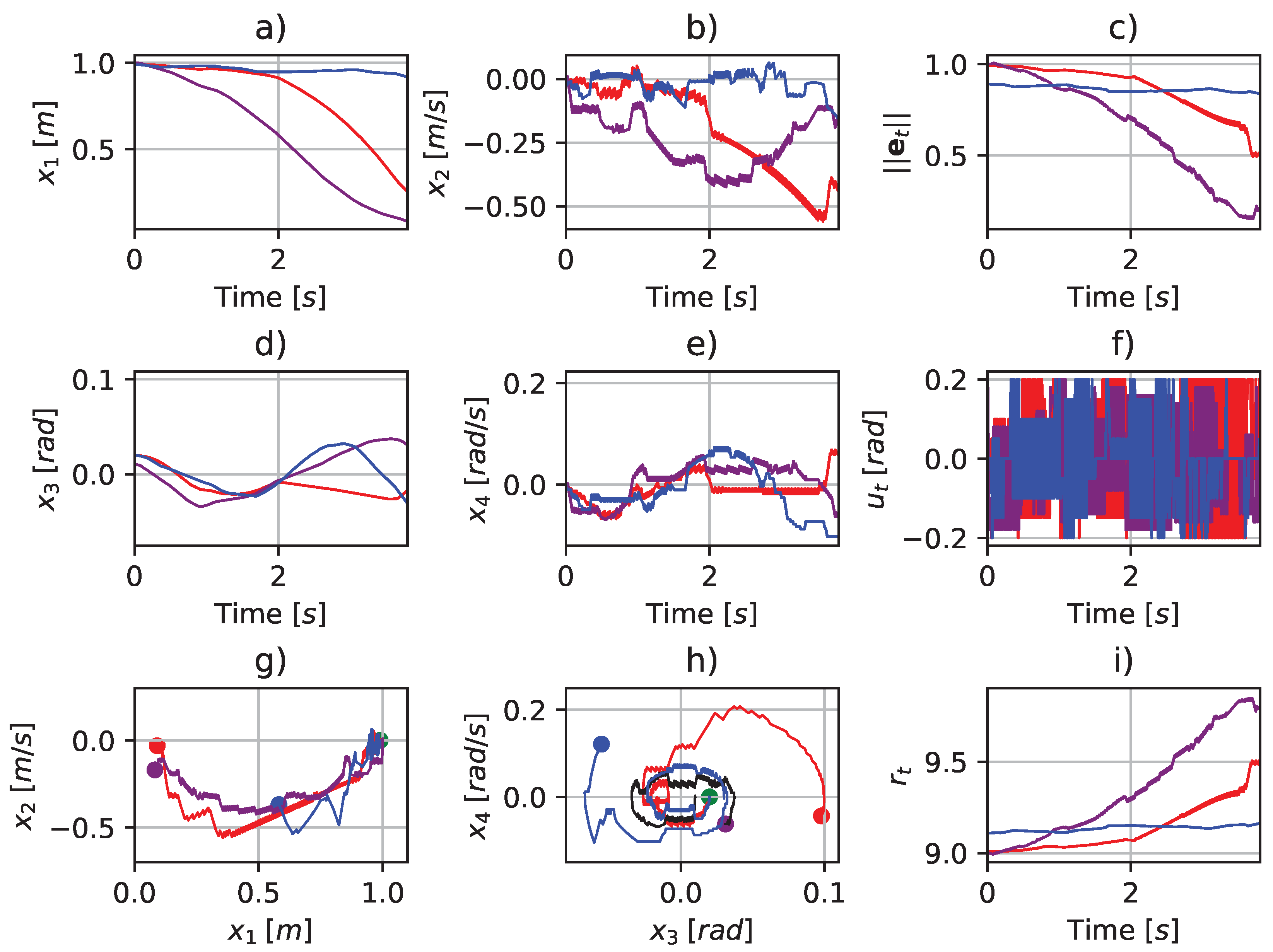
Three conditions are simulated for comparative purposes to show the performance of the Q-learning algorithm in learning the rocket landing. The simulation:

1.

shows the comparative performance of the classical and variable box methods for the same output limits, action space, and number states but with different resolutions.

2.

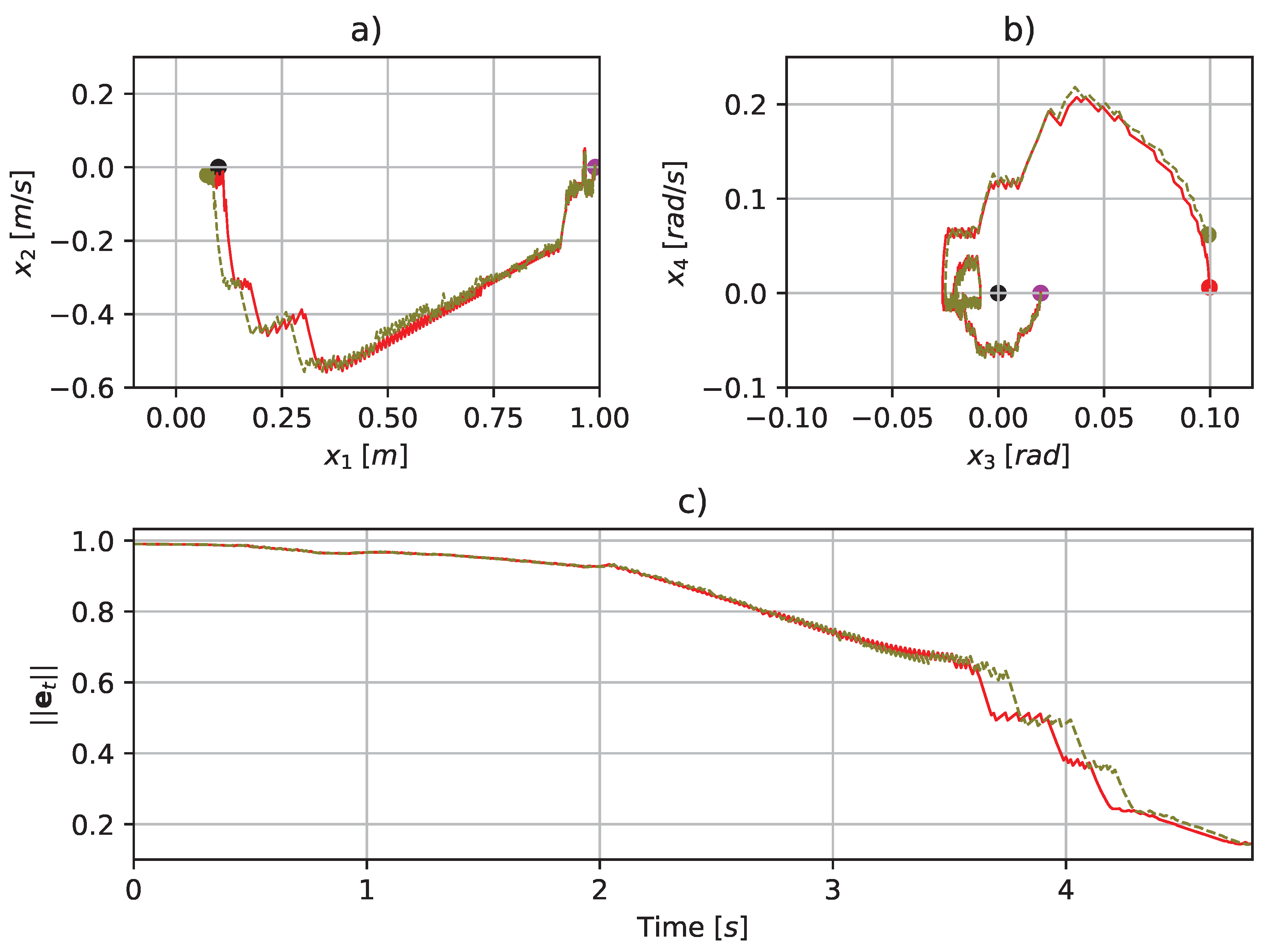
shows the comparative performance considering the same goal-box resolution and state-space dimension for the variable box method.

3.

shows the rocket landing trajectories when the rocket is subject to a Gaussian disturbance.

The simulator was written in Python, with a step size of $h=0.01$ [s]. The principal modules were numpy to compute the math operations, matplotlib to depict the results, and our Q-learning algorithm, which was embedded in the “temporal difference” module.

The task was to learn the vertical rocket landing from an arbitrary initial condition ${\mathbf{y}}_0$ to ${\mathbf{y}}_t^d=[0.1,0,0,0]$, see Figure 5. Note that offset was set due to the landing train and the command was implemented using only the nozzle angle.

The reward assignment was designed as follows:

$$\begin{array}{c}\hfill R_t\left({\mathbf{e}}_t\right)=\left\{\begin{array}{ccc}10-\left|\right|{\mathbf{e}}_t\left|\right|\hfill & \mathrm{if}{\mathbf{y}}_t\mathrm{is}\mathrm{within}\mathrm{limits}\hfill & (\mathrm{it}\mathrm{awards})\hfill \\ -1000\hfill & \mathrm{otherwise}\hfill & (\mathrm{it}\mathrm{penalizes})\hfill \end{array}\right.\end{array}$$

(15)

where ${\mathbf{e}}_t={\mathbf{y}}_t^d-{\mathbf{y}}_t$ is the error vector and $\left|\right|·\left|\right|$ is the Euclidean norm. Function $R_t\left({\mathbf{e}}_t\right)$ increases as $\left|\right|{\mathbf{e}}_t\left|\right|\to 0$, maximizing the reward, i.e., ${\mathbf{y}}_t\to {\mathbf{y}}_t^d$.

4.4. Rocket and Learning Parameters

The rocket parameters used were those of the Saturn V rocket from NASA [19], where $N_{\alpha }=4.46477$ [N], $A=6.09525$ [N], $m_r=570\times {10}^3$ [kg], $T=7.605\times {10}^6$ [N], $X_{gim}=21$ [m], $X_{cp}=10$ [m], $J_{yy}=3.2\times {10}^7\left[\mathrm{kg}{\mathrm{m}}^2\right]$, $J_2=1.0826\times {10}^{-3}$, $\mu =3.986\times {10}^{14}\left[\frac{{\mathrm{m}}^3}{{\mathrm{s}}^2}\right]$, $R_0=6.371\times {10}^6$ [m], $r_e=6.372\times {10}^6$ [m], ${\alpha }_{{\omega }_{\theta }}=0$ [rad], and ${\gamma }_{\theta }=\dot{\mathrm{z}}/\mathrm{V}$, with $V=400\left[\frac{\mathrm{m}}{\mathrm{s}}\right]$. The learning parameters were $\gamma =0.7$ and ${\alpha }_Q=0.01$ for $5\times {10}^6$ episodes. The first and second simulations were disturbed with ${\mathit{\eta }}_t={[0,0]}^T$.

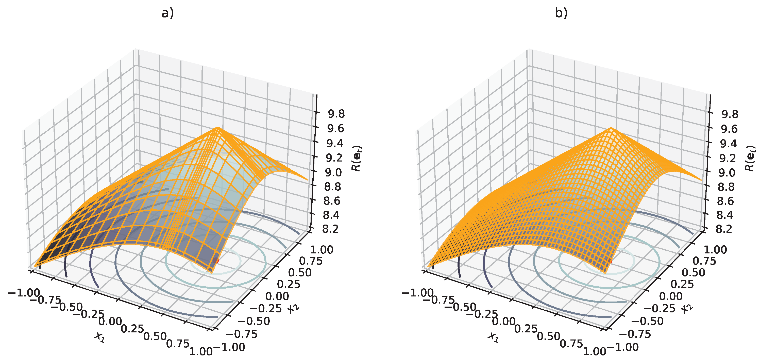
4.5. Simulation A: Comparative Performance

Consider the output limits $[y_1,y_2]\in [-1,1]$ [m, m/s] and $[y_3,y_4]\in [-0.5,0.5]$ [rad,  rad/s], the action space $u_t\in [-0.2,0.2]$ [rad], and 9 number states for both the classical and variable box methods. For the classical box method CBM1, the constant resolutions were ${ϵ}_{y_1}={ϵ}_{y_2}=3\times {10}^{-2}$ and ${ϵ}_{y_3}={ϵ}_{y_4}=8\times {10}^{-2}$. The first and last box indexes were considered open range ($\pm \infty$) as in membership functions in classical fuzzy logic. Then, there arose 28,224 number states. On the other hand, two sets of variable box parameters were tuned for the variable box method: (a) VBM1: The goal-box resolution was ${ϵ}_{y_1}={ϵ}_{y_2}={ϵ}_{y_3}={ϵ}_{y_4}=1\times {10}^{-2}$, with 28,224 number states as in CBM1. The action space used 21 action boxes. (b) VBM2: The goal-box resolution was the same as VBM1 but the output limits were set at $[y_1,y_2]\in [-10,10]$ [m, m/s] and $[y_3,y_4]\in [-0.5,0.5]$ [rad, rad/s], producing 51,984 number states. The action space also used 21 action boxes.

Figure 6 shows the results using CBM1, VBM1, and VBM2. The initial conditions for all cases were ${\mathbf{x}}_0=[0.99\mathrm{m},$ $0\mathrm{m}/\mathrm{s},$ $0.02\mathrm{rad},$ ${0\mathrm{rad}/\mathrm{s}]}^T$, for  ${ϵ}_{gb}=1\times {10}^{-2}$. Simulations CBM1 and VBM1 needed $dim\left(\mathcal{S}\right)=$ 28,224 and VBM2 requires $dim\left(\mathcal{S}\right)=$ 51,988 to converge faster ($t_{land}=3.7$ [s]); however, the highest reward ($r_{max}=9.8618$) with the lower error norm ($\left|\right|{\mathbf{e}}_t{\left|\right|}_{min}=0.1381$) is obtained with VBM1, showing that in any case, the proposed variable method performs better than the constant method, see

Table 1. Comparative study results between CBM and VBM under different conditions of the goal-box resolution and state-space dimension. The best metrics (${ϵ}_{gb},\left|\right|{\mathbf{e}}_t{\left|\right|}_{min},r_{max},t_{land}$ [s]) were obtained with VBM4 at the expense of a higher computational load ($dim\left(\mathcal{S}\right)=$ 51,984).

Box Method	Code	${\mathit{ϵ}}_{\mathbf{gb}}$	$dim\left(\mathcal{S}\right)$	$\left|\right|{\mathit{e}}_{\mathit{t}}{\left|\right|}_{min}$	${\mathit{r}}_{\mathit{max}}$	${\mathit{t}}_{\mathit{land}}\left[\mathbf{s}\right]$
Classical	CBM1	$1\times {10}^{-2}$	28,224	0.6304	9.3787	4.88
Variable	VBM1	$1\times {10}^{-2}$	28,224	0.1381	9.8618	4.82
Variable	VBM3	$5\times {10}^{-2}$	18,225	0.1519	9.8480	4.93
	VBM2	$1\times {10}^{-2}$	51,984	0.1458	9.8541	3.7
	VBM4	$1\times {10}^{-3}$	51,984	0.0867	9.9132	3.22

.

In Figure 6a,b,d,e, it can be seen that while the rocket is descending, the height velocity $x_2$, angle $x_3$, and angle velocity $x_4$ remain bounded. In addition, it can be seen that the state-variable errors are near zero, which is typical of reinforcement learning algorithms. Additionally, Figure 6a shows that the set of simulations using the variable box method had better landing performance than the classical box method. Furthermore, Figure 6f shows that the control signal $u_t$ of the classical box method had a limited correlation between actions, states, and rewards, which limited the adequate exploration of the state space. Overall, the second set of simulation parameters with VBM2 performed better (as indicated in purple in Figure 6) at the expense of a significant increase in the number states. Finally, Figure 6g,h presents the portrait phase for each set of simulations, showing the convergence for the three cases; however, in the variable box method, the rocket approached smoothly due to the mesh’s density.

4.6. Simulation B: Comparative Performance

We aimed to compare the landing performance using the classical and variable box methods based on three parameters: the minimum norm error $\left|\right|{\mathbf{e}}_t{\left|\right|}_{min}$; maximum reward obtained $r_{max}$; and time taken to land $t_{land}$. The parameters were the goal-box resolution ${ϵ}_{gb}$ and state-space dimension $dim\left(\mathcal{S}\right)$ tuned by safety resolution ${ϵ}_s$, see Table 1. The initial conditions were ${\mathbf{x}}_0={[0.99\mathrm{m},0\mathrm{m}/\mathrm{s},0.02\mathrm{rad},0\mathrm{rad}/\mathrm{s}]}^T$.

The first two rows in Table 1 correspond to the results presented in Figure 6, where VBM1 achieved better performance than CBM1 using the same state-space dimension (28,224) and box resolution. VBM3 showed acceptable performance with only 18,225 (in bold) number states, which caused increasing errors and a poor reward; moreover, the landing time was the worst. Additionally, in VBM2, the state-space dimension increased to 51,984 due to the loose-fitting grid around the learning goal, the errors decreased slightly, and the landing took place in $3.7$ [s].

If the goal-box resolution was defined as $1\times {10}^{-3}$, it yielded 51,984 number states and the best performance was achieved (in bold) in terms of the error, reward, and landing time, see VBM4 in Table 1. Note that when applying the variable box method, it is suggested to establish a compromise among the learning goal, goal-box resolution, and state-space dimension on a trial-and-error basis.

4.7. Rocket Subject to Disturbances

Consider the rocket subject to a Gaussian disturbance $N_G(·)$ such that ${\eta }_{t,1}={\eta }_{t,2}=\kappa N_G({\mu }_G,{\sigma }^2)$ for ${\mu }_G=0$, $\sigma =1$, and $\kappa =8\times {10}^{-2}\left[N\right]$. Figure 7 shows the performance of the rocket landing with and without perturbations using the policy of the VBM1 case defined in Section 4.5. The initial conditions were ${\mathbf{x}}_0=[0.99\mathrm{m},$$0\mathrm{m}/\mathrm{s},$$0.02\mathrm{rad},$${0\mathrm{rad}/\mathrm{s}]}^T$. Figure 7a,b show the rocket’s portrait phase reaching the goal. Figure 7c shows the convergence under the previous learning process conditions, which were sufficient to compensate for disturbances that were unknown a priori.

5. Conclusions

The classical Q-learning scheme guarantees iteratively reaching the goal states with a quasi-optimal policy. This powerful scheme seems promising for complex dynamical tasks such as landing a massive rocket but requires improved maneuverability. The variable box method is proposed for the Q-learning algorithm to yield higher resolution near the target region, where higher accuracy is required, such as the landing pad. In addition, this method suggests that asymmetric refinement may be introduced at different state regions in terms of the error threshold depending on the available computational power. This way, the learning process emerges with the refinement of boxes to actions without significantly increasing the computational costs. Simulations show how convenient it is to explore such refinements of box-sizing instead of increasing the number of boxes. In addition, the proposed variable box method can be introduced into other RL algorithms since the Q-learning architecture is maintained.

Due to the Q-learning algorithm being an offline learning scheme, a sample of the whole system behavior throughout the finite state-number space, which an expert user should tune on a trial-and-error basis, is needed to asymptotically compute the quasi-optimal policy rewarded by $r_t$. Once that quasi-optimal policy is learned offline, it is necessary to switch to an expert agent who already knows a local quasi-optimal policy ${\pi }_{\ast }\left(s_t\right)$. Moreover, caution is advised since, in practice, slight changes in states and actions lead to a slightly different policy, i.e., $\pi \left(s_t\right)\ne {\pi }_{\ast }\left(s_t\right)$. Thus, it is customary to run many simulation tests beforehand to “average” the policy $\widehat{\pi }\left(s_t\right)$ tested in real systems, where $\widehat{\pi }\left(s_t\right)\approx {\pi }_{\ast }\left(s_t\right)$. In our case, the proposed variable box method may assist in practice since it produces smoother but finer actions for larger errors.

References

1. Nebylov, A.; Nebylov, V. Reusable Space Planes Challenges and Control Problems. IFAC-PapersOnLine 2016, 49, 480–485. [Google Scholar] [CrossRef]
2. Ünal, A.; Yaman, K.; Okur, E.; Adli, M.A. Design and Implementation of a Thrust Vector Control (TVC) Test System. J. Polytech. Politek. Derg. 2018, 21, 497–505. [Google Scholar] [CrossRef]
3. Oates, G.C. Aerothermodynamics of Gas Turbine and Rocket Propulsion, 3rd ed.; American Institute of Aeronautics and Astronautics: Washington, DC, USA, 1997; ISBN 978-1-56347-241-1. [Google Scholar]
4. Chen, Y.; Ma, L. Rocket Powered Landing Guidance Using Proximal Policy Optimization. In Proceedings of the 4th International Conference on Automation, Control and Robotics Engineering, Shenzhen, China, 19–21 July 2019; pp. 1–6. [Google Scholar] [CrossRef]
5. Yuan, H.; Zhao, Y.; Mou, Y.; Wang, X. Leveraging Curriculum Reinforcement Learning for Rocket Powered Landing Guidance and Control. In Proceedings of the China Automation Congress, Beijing, China, 22–24 October 2021; pp. 5765–5770. [Google Scholar] [CrossRef]
6. Sánchez-Sánchez, C.; Izzo, D. Real-Time Optimal Control via Deep Neural Networks: Study on Landing Problems. J. Guid. Control Dyn. 2018, 41, 1122–1135. [Google Scholar] [CrossRef]
7. Zhang, L.; Chen, Z.; Wang, J.; Huang, Z. Rocket Image Classification Based on Deep Convolutional Neural Network. In Proceedings of the 10th International Conference on Communications, Circuits and Systems, Chengdu, China, 22–24 December 2018; pp. 383–386. [Google Scholar] [CrossRef]
8. Stengel, R.F. Flight Dynamics; Princeton University Press: Princeton, NJ, USA, 2004; ISBN 978-1-40086-681-6. [Google Scholar]
9. Sutton, R.S.; Barto, A.G. Reinforcement Learning: An Introduction, 2nd ed.; A Bradford Book: Cambridge, MA, USA, 2018; ISBN 978-0-262-03924-6. [Google Scholar]
10. Michie, D.; Chambers, R.A. Boxes: An Experiment in Adaptive Control. Mach. Intell. 1968, 2, 137–152. [Google Scholar]
11. Davies, S. Multidimensional Triangulation and Interpolation for Reinforcement Learning. In Proceedings of the 9th International Conference on Neural Information Processing Systems, Denver, CO, USA, 3–5 December 1996; pp. 1005–1011. [Google Scholar] [CrossRef]
12. Dayan, P.; Hinton, G.E. Feudal Reinforcement Learning. In Proceedings of the Advances in Neural Information Processing Systems 5, Denver, CO, USA, 30 November–3 December 1992; pp. 271–278. [Google Scholar] [CrossRef]
13. Barto, A.G.; Sutton, R.S.; Anderson, C.W. Neuronlike Adaptive Elements that Can Solve Difficult Learning Control Problems. IEEE Trans. Syst. Man Cybern. 1983, SMC-13, 834–846. [Google Scholar] [CrossRef]
14. Munos, R.; Moore, A. Variable Resolution Discretization in Optimal Control. Mach. Learn. 2002, 49, 291–323. [Google Scholar] [CrossRef]
15. Moore, A.W. Variable Resolution Dynamic Programming: Efficiently Learning Action Maps in Multivariate Real-valued State-spaces. In Proceedings of the 8th International Conference of Machine Learning, Evanston, IL, USA, 1 June 1991; pp. 333–337. [Google Scholar] [CrossRef]
16. Zahmatkesh, M.; Emami, S.A.; Banazadeh, A.; Castaldi, P. Robust Attitude Control of an Agile Aircraft Using Improved Q-Learning. Actuators 2022, 11, 374. [Google Scholar] [CrossRef]
17. Sutton, R.S. First Results with Dyna, an Integrated Architecture for Learning, Planning and Reacting. In Neural Networks for Control; Miller, W.T., Sutton, R.S., Werbos, P.J., Eds.; The MIT Press: Cambridge, MA, USA, 1991. [Google Scholar]
18. Tewari, A. Atmospheric and Space Flight Dynamics; Modeling and Simulation in Science, Engineering and Technology; Birkhäuser Boston: Boston, MA, USA, 2007; ISBN 978-0-81764-437-6. [Google Scholar] [CrossRef]
19. Martínez-Perez, I.; Garcia-Rodriguez, R.; Vega-Navarrete, M.A.; Ramos-Velasco, L.E. Sliding-mode based Thrust Vector Control for Aircrafts. In Proceedings of the 12th International Micro Air Vehicle Conference, Puebla, Mexico, 16–20 November 2021; pp. 137–143. [Google Scholar]
Figure 1. Conceptual reinforcement learning scheme.
Machines 11 00214 g001
Figure 2. Level sets for vertical rocket landing were obtained with (a) the variable box method using 576 boxes, and (b) the classical box method using 40,000 boxes, both tuned to obtain similar final results. The dramatic reduction in the number of boxes achieved using our proposed variable method results from the symmetrical higher resolution around the goal box, which yields a higher reward in areas with zero errors.
Machines 11 00214 g002
Figure 3. Schematic diagram of the proposed variable box method with Q-learning. Two feedback loops reinforce the intertwined closed-loop dynamic interplay of the expert agent to guarantee y t y t d , whereas the cumulative reward r t is maximized.
Machines 11 00214 g003
Figure 4. (a) Rocket with an integrated TVC, with a bounded angle nozzle, and the aerodynamics forces shown in (b) the xz-plane, and (c) the yz-plane. Notice that CoG and CoP are at different locations, which yields a rather highly nonlinear coupled non-affine underactuated system.
Machines 11 00214 g004
Figure 5. Schematic showing the task goal: learn the optimal admissible rocket trajectories for landing from an arbitrary initial condition x 0 to a (constant) desired landing spot y d t .
Machines 11 00214 g005
Figure 6. Comparative results for landing a rocket: classical box method CBM1 (blue), variable box method VBM1 (red), and VBM2 (purple), where the purple and black dots represent the initial and desired conditions, respectively. Subfigures depict the following: (a,b,d,e) show the rocket descending phase, for height velocity x 2 , angle x 3 , and angle velocity x 4 remain bounded while tracking errors remain near zero; (a) shows the better performance of our proposal, (c) shows how the error norm decreases while the reward increases (i), the control signal performance u t is show in (f), and phase portraits are show in (g,h).
Machines 11 00214 g006
Figure 7. Rocket landing trajectories shown in phase portraits ((a) height position versus its velocity, and (b) angular position versus its velocity) using the proposed variable box method without disturbances (red) and subject to a disturbance η t (olive). The purple and black dots represent the initial and desired conditions, respectively. Remarkably, L 2 norm of errors (c) yields similar plots, showing trajectories are learned for both cases, despite the strong disturbance (olive) at the expense of a slight (admissible) final deviation.
Machines 11 00214 g007