Article

Dynamic Modeling and Model-Based Control with Neural Network-Based Compensation of a Five Degrees-of-Freedom Parallel Mechanism

1
School of Aerospace Engineering and Applied Mechanics, Tongji University, Shanghai 200092, China
2
Department of Mechanical Engineering, Tsinghua University, Beijing 100084, China
*
Author to whom correspondence should be addressed.
Machines 2023, 11(2), 195; https://doi.org/10.3390/machines11020195
Submission received: 13 December 2022 / Revised: 27 January 2023 / Accepted: 30 January 2023 / Published: 1 February 2023
(This article belongs to the Special Issue Development and Applications of Parallel Robots)

Abstract

:
In this paper, a spatial parallel mechanism with five degrees of freedom is studied in order to provide a promising dynamic model for the control design. According to the inverse kinematics of the mechanism, the dynamic model is derived by using the Lagrangian method, and the co-simulation using MSC ADAMS and MATLAB/Simulink is adopted to verify the established dynamic model. Then the pre-trained deep neural network (DNN) is introduced to predict the real-time state of the end-effector of the mechanism. Compared to the traditional Newton’s method, the DNN method reduces the cost of the forward kinematics calculation while ensuring prediction accuracy, which enables the dynamic compensation based on feedback signals. Furthermore, the computed torque control with DNN-based feedback compensation is implemented for the trajectory tracking of the mechanism. The simulations show that, in the most complicated case that involves friction and external disturbance, the proposed controller has better tracking performance. The results indicate the necessity of dynamic modeling in the design of control with high precision.

1. Introduction

As a powerful supplement to the traditional serial open-loop mechanisms, the closed-loop parallel mechanisms have many advantages in accuracy, speed, and payload ability. However, the parallel mechanisms also suffer from limb interferences and a large number of singularities inside their workspaces, which seriously impedes the extensive application of parallel mechanisms [1]. Therefore, spatial movement capability is crucial to evaluate the performance of spatial parallel mechanisms (PMs) [2,3]. The general spatial PMs have many successful configurations with three degrees of freedom (DoF), such as the classical spatial DELTA mechanism [4], the 3-PSP spatial PMs [5], the 1-UP&2-UPS spatial PMs [6], and the 2R1T parallel end-effector head mechanism [7], etc. One disadvantage of 3-DoF spatial PMs is that they do not adapt well to complex working conditions. Nowadays, PMs are developing towards more DoF and more actuations. More actuations tend to generate kinematic redundancy in PMs, which is an effective way to improve the dynamic performance of the mechanism [8] and avoid singular configurations [9]. which provides more possibilities for the design of PMs. More DoF enables the PMs to adapt to complex working conditions. Therefore the spatial PMs with more degrees of freedom are attracting more attention [10]. For example, the spatial PM with 5-DoF has been successfully applied in tasks such as the machining of large aircraft structural components and the assembly of parts with high precision and etc. [11]. Obviously, one crucial issue of such a task is the design of a control scheme that bounds the tracking error and consequently guarantees the positioning accuracy [12].
In recent years, the high-precision motion control for spatial PMs have been widely investigated by scholars [13,14]. For the control of a novel reconfigurable parallel mechanism, Huang [15] designed a fuzzy-proportion integration differentiation (PID) controller to track the trajectory of the end-effector. However, the proposed fuzzy-PID controller did not include dynamic compensation terms, and consequently, the tracking accuracy of the mechanism might be limited. The model-based control, which improves control performance and eliminates steady-state errors of the mechanism by compensating the dynamic interference, has been widely used in controlling spatial PMs, and the results have revealed the superiority of model-based control [16,17].
Dynamic modeling, as the basis of dynamic performance analysis of mechanisms, is the core of the structural parameters design and model-based control of parallel mechanisms. Compared with serial open-loop mechanisms, the kinematics analysis, which plays the fundamental role of dynamic modeling, is not an easy task for the spatial PMs due to their multi-closed-loop configuration, especially for spatial PMs with multiple DoF. In previous research, the dynamic model of spatial PMs are usually established by means of the Newton–Euler approach, Lagrangian method, the principle of virtual work, and Kane approach, etc. The Newton–Euler approach is the most commonly used dynamic modeling method for spatial PMs [18,19]. Since the Newton–Euler approach is a recursive derivation method based on vector mechanics, it has a clear physical meaning and geometric explanation. However, as the complexity of the mechanism increases, the Newton–Euler approach requires more differential-algebraic equations to formulate the model [20]. Compared with Newton–Euler approach, the Lagrangian method is based on the calculation of kinetic energy and potential energy of the system and consequently avoids the calculation of constraint forces, but the symbolic derivation of the matrix form of the Lagrange equation is quite complicated. Similar to the Lagrangian method, the principle of virtual work can also avoid the calculation of constraint forces of the mechanism. However, the modeling process of this method is featured by the velocity transform between joint and task spaces, which brings much inconvenience in forward dynamics analysis for some spatial PMs [11]. Another classic approach to multi-body system dynamics modeling is the Kane method, which has the advantages of both vector mechanics and analytical mechanics, especially in the modeling of nonholonomic systems. Using the Kane approach, Yang [21] investigated the full dynamic model of an spatial PM system and derived the simplified dynamic model through the rigid body decomposition method. The main challenge of applying the Kane method is the lack of a uniform framework, which results in a decrease in computational efficiency, especially for complex spatial PMs.
Based on the dynamic model of spatial PMs, the model-based control has been successfully applied in many types of research, most of which are model-based feedforward control [22,23]. Since the feedforward control is categorized as open-loop control, it is difficult to realize full compensation when there are many disturbance factors in the system. Therefore, it is necessary to introduce feedback dynamic compensation into real-time control. However, the feedback compensation control for spatial PMs requires the state of motion of the end-effector, which can only be obtained by means of the forward kinematics calculation when lacking real-time measurements with high precision. In other words, given the feedback of the state of motion of driving elements, one needs to calculate the state of the end-effector so as to compare with its desired state within the control loop.
Contrary to the serial mechanism, the inverse kinematics of a parallel mechanism is usually simple and straightforward [24,25]. However, the forward kinematics of parallel mechanism involves highly coupled nonlinear equations, which makes it difficult to find analytical solutions. To tackle this problem, Asier [26] added extra sensors to the passive joints of the parallel robot. At the same time, the cost of the experiment and the complexity of data transmission will increase greatly. Some analytical methods are used to establish the forward kinematics model of parallel mechanisms with certain configurations [27,28]. While most of the theoretical methods are limited to parallel mechanisms with a special configuration, numerical approaches are employed to solve forward kinematics of parallel mechanisms of arbitrary type. However, the convergence of the Newton–Raphson based algorithm, the most widely used numerical scheme for solving forward kinematics, depends on the selection of the initial value. When the initial value is not close to the exact solution, the algorithm will take a long time to converge or even diverge. In recent years, artificial intelligence approaches have been widely applied for their promising global performance. Nouri Rahmat Abadi, B. and Carretero, J.A. [29] successfully perform the real-time motion planning of a class of kinematically redundant PMs using the multilayer perceptron-based neural network (MLP). Zhang [30] compares the performance of different artificial intelligence approaches to solve the forward kinematics of an actuation redundant parallel manipulator, which provides guidance for the application of artificial intelligence approaches to the forward kinematics problem of parallel robots. Given sufficient training data, the mapping from states of driving components to states of end-effector can be accurately established with the aid of the strong capability of function approximation of the neural network [31].
In this paper, the dynamic model of a machining robot, abstracted as a spatial PM with 5-DoF, is studied to provide the foundation of the model-based control. Given appropriately selected generalized coordinates of the spatial PM, the Lagrangian method is adopted to formulate the model of the spatial PM of concern. Note that the main challenge of the feedback control with dynamic compensation for the spatial PM under consideration is the real-time calculation of the forward kinematics, we propose to predict the real-time state of the end-effector by a deep neural network (DNN) to speed up the forward kinematics analysis. Afterward, the feedback control with dynamic compensation can be designed based on the dynamic model implemented by the end-effector state predictor based on DNN.
The rest of the paper is organized as follows. In Section 2, we briefly introduce the structure of the mechanism and analyze its inverse kinematics. In Section 3, based on the kinematic analysis, we use the Lagrangian method to establish the dynamic model of the proposed spatial PM, and then we run the co-simulation by using MSC ADAMS and MATLAB/Simulink to verify the dynamic model. In Section 4, we use the inverse kinematics of the mechanism to generate a training data set, and then train an artificial neural network to represent the solution of the forward kinematics. On this basis, we design a computed force control law with dynamic feedback compensation. Then the numerical simulations of the computed force control, the feedforward control, and the PD control of the spatial PM are provided. The simulation results show that the proposed control law has better performance of dynamic tracking.

2. Structure Description and Kinematics Analysis

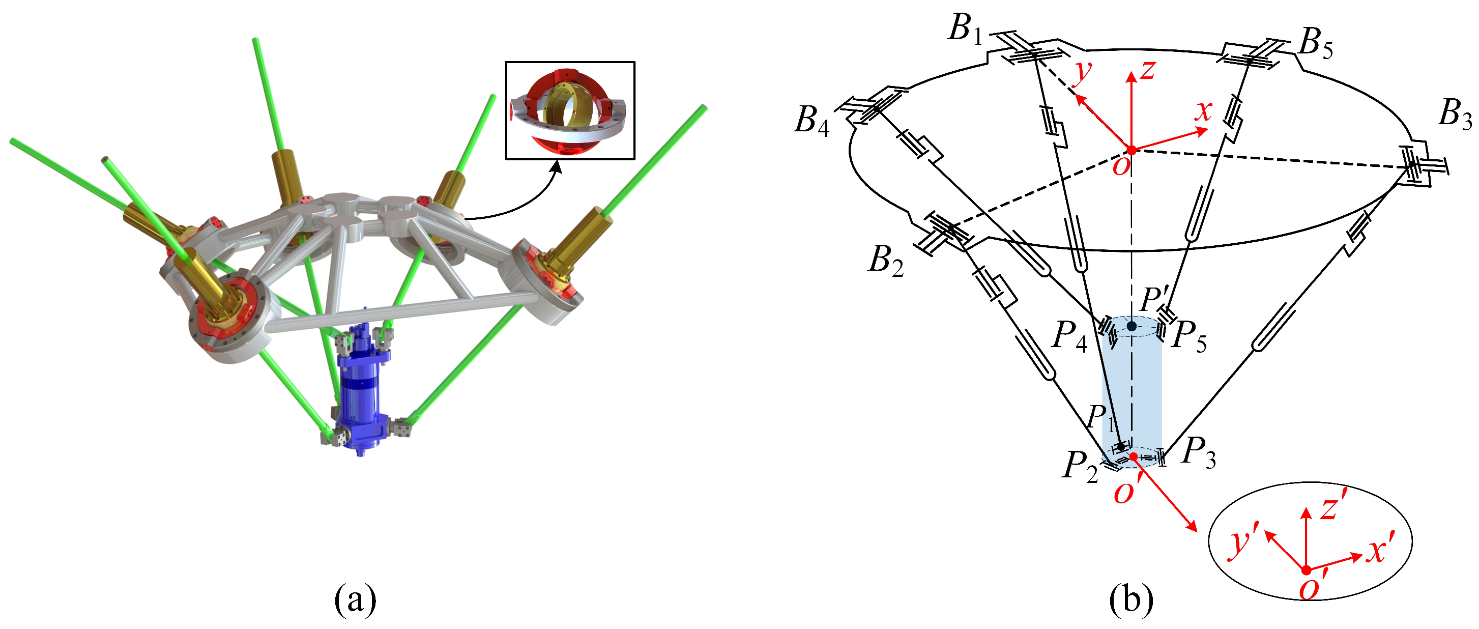
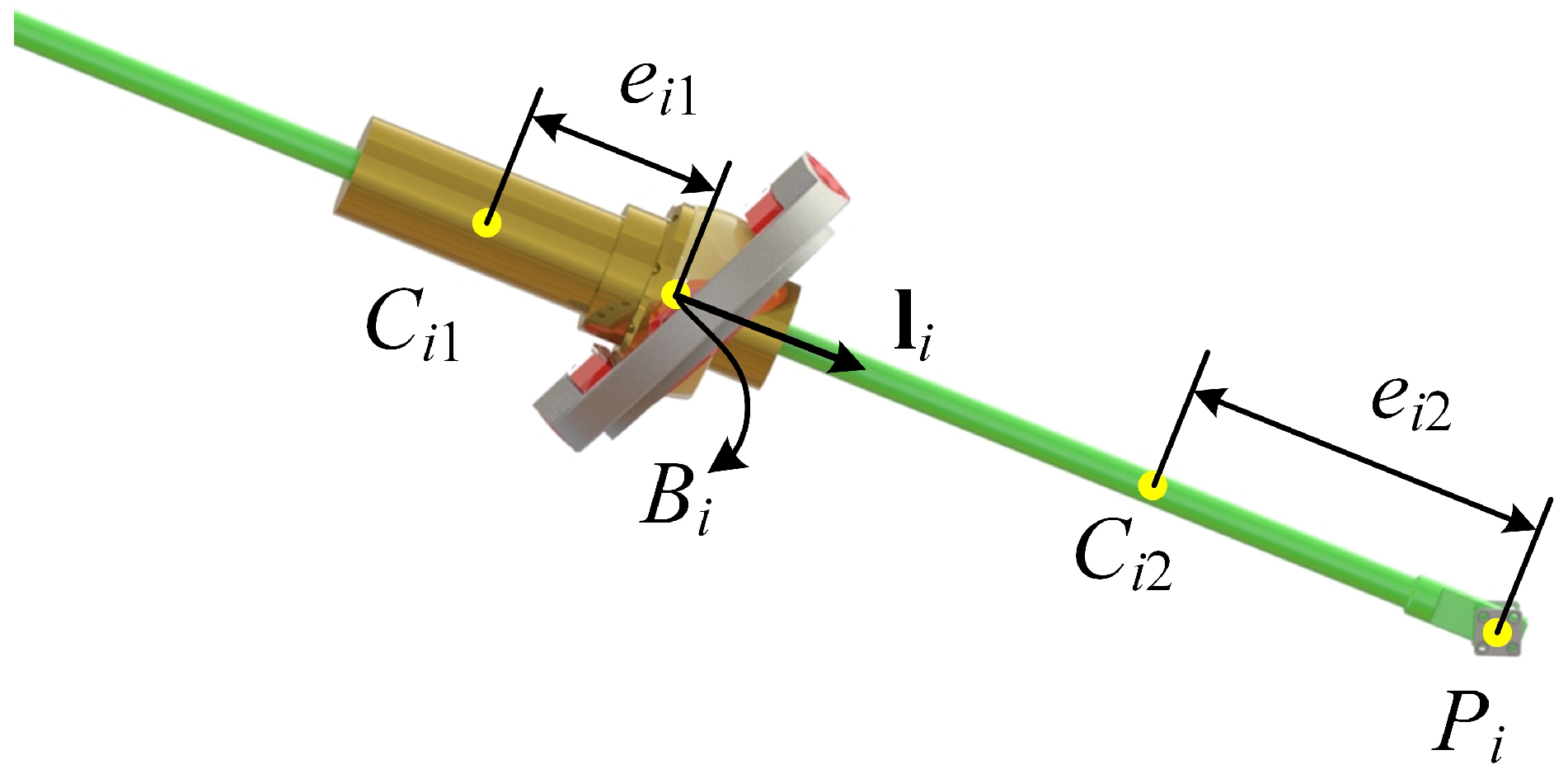
2.1. Structure Description

Figure 1 depicts the configuration of the SPM under consideration, appearing as the prototype of a portable machining robot. The spatial PM is composed of a base, an end-effector, and five limbs. As shown in Figure 1b, B i ( i = 1 , 2 , , 5 ) are spherical joints in the structure. In accordance with descriptions of previous works where the 5-DoF mechanism was already introduced, the universal joint on each sleeve and the spinning motion of each ball screw are collectively equivalent to a spherical joint. The first limb is an SPR kinematic chain (S-spherical joint; P- active prismatic joint; R-revolute joint), and the remaining four limbs are SPU kinematic chains (U- universal joint), thus the spatial PM can be represented as SPR-4(SPU). The SPR kinematic chain imposes a constraint force to the end-effector, and the SPU kinematic chains have no constraint on the end-effector. Actuated by five prismatic inputs, the end-effector of the spatial PM is endowed with five DoF, including three translational DoF and two rotational DoF, and the detailed analysis can be found in Ref. [32].

2.2. Inverse Position Analysis

In order to express the dynamics of the mechanism in terms of the task-space coordinates, one needs to figure out how the limb’s state changes with the end-effector state. As shown in Figure 1b, the kinematics of the 5-DoF spatial PM can be described by two coordinate systems: the global coordinate system : o x y z which is mounted on the center of the base, and the co-rotational coordinate system : o x y z which is mounted on the bottom center of the end-effector. Denote by T = oo = x , y , z T the position of the bottom center of the end-effector in the global coordinate system. The base is coplanar with the o x y plane, where o is the center of the circle consisting of points B 1 , B 2 , B 3 , B 4 and B 5 . The y a x i s in the global coordinates is collinear with o B 1 , and the y a x i s in the co-rotational coordinate system is collinear with o P 1 . The vectors P 2 P 4 , P 3 P 5 are parallel to o P , i.e., the central axis of the end-effector. Denote the length of ball screw by l t o t a l and let o B i = R 1 , ( i = 1 , 2 , 3 , 4 , 5 ) , o P i = R 2 , ( i = 1 , 2 , 3 ) , o P = H , B 1 o B 2 = B 1 o B 3 = B 2 o B 3 = 2 π 2 π 3 3 , B 1 o B 4 = B 1 o B 5 = π π 4 4 . The detailed expressions for the position of B i ( i = 1 , 2 , , 5 ) in : o x y z and P i ( i = 1 , 2 , , 5 ) in : o x y z are given in Appendix A.
In Ref. [32], the orientation of the end-effector is represented by tilt-and-torsion (T&T) angles, which may result in the singularity of Jacobian matrix in some common orientation of the end-effector, i.e., vertical state. Differently from previous work, the RPY angles are used to represent the orientation of the end-effector to avoid such phenomenon. We define β as the roll angle, γ as the pitch angle, and α as the yaw angle. Under the description of RPY angles, the rotation matrix of the end-effector with respect to the fixed base platform can be expressed as
R α , β , γ = R z ( β ) R y ( γ ) R x ( α ) = cos β cos γ sin α cos β sin γ cos α sin β cos α cos β sin γ + sin α sin β sin β cos γ sin α sin β sin γ + cos α cos β cos α sin β sin γ sin α cos β sin γ sin α cos γ cos α cos γ .
Due to the constraint of the first limb, B 1 , P 1 , o , p will be restricted in the same plane. This condition can be expressed as follows [33]:
( o p × o p 1 ) · o B 1 = 0 ,
where
o p = R α , β , γ 0 , 0 , H T , o B 1 = x , y R 1 , z T , o P 1 = R α , β , γ 0 , R 2 , H T .
It can be obtained from Equation (3) that
z sin γ + R 1 cos γ sin β x cos γ cos β y cos γ sin β = 0 ,
which yields
γ = arctan x cos β + y sin β R 1 sin β z ± π 2 ,
indicating that the DoF of the proposed spatial PM is five. From Equations (1) and (5), R can be calculated for certain coordinates of task space, i.e., ( x , y , z , α , β ) . Then the coordinates of P i ( i = 1 , 2 , , 5 ) in the global frame can be expressed as
P i = R ( α , β , γ ) P i + T .
The coordinates of the joint space can be expressed as L = l 1 l 2 l 3 l 4 l 5 T . Let l i = B i P i , i = 1 , , 5 , i.e., l i represents the screw length of each linear drive. Together with the position of B i ( i = 1 , 2 , , 5 ) and Equation (6), we have completed the inverse kinematics analysis by formulating the mapping from ( x , y , z , α , β ) to l i , i = 1 , , 5 .

2.3. Velocity Analysis and Jacobian Matrix

In this part, we use the Jacobian matrix to analyze the velocity relationship between the end-effector and the input limb. The structure of input limb B i P i ( i = 1 , 2 , , 5 ) is shown in Figure 2, where l i represents the unit vector in the corresponding direction of the ith limb, and e i 1 , e i 2 represent, respectively, the centroid position of the sleeve and the limb. It is obvious that
o B i + B i P i = oo + o P i .
Since oo = T , B i o = B i , B i P i = l i l i , and o P i = R α , β , γ P i , Equation (7) can be rewritten as
l i l i + B i = T + R α , β , γ P i .
Figure 2. Structure and kinematic scheme of input ith limb.
Machines 11 00195 g002
Based on Equation (8), one can establish the relationship between the velocity in the joint space and that of the task space. To this end, we first note that
R T R ˙ = 0 ω z ω y ω z 0 ω x ω y ω x 0 ,
where ω x ω y ω z T = : ω p represents the angular velocity of the end-effector. Denoting by ω i the angular velocity of the limb, and differentiating both sides of Equation (8) with respect to time yield
l ˙ i l i + l i ( ω i × l i ) = T ˙ + ω p × R ( α , β , γ ) P i ,
Based on Equation (10), a direct calculation shows that
l ˙ i l i + L i ( ω i × l i ) × l i = T ˙ + ω p × R ( α , β , γ ) P i × l i , ω i = T ˙ + ω p × R ( α , β , γ ) P i × l i l i .
and
l i · l ˙ i l i + L i ( ω i × l i ) = l i · T ˙ + ω p × R ( α , β , γ ) P i , l ˙ i = T ˙ · l i + ω p × R ( α , β , γ ) P i · l i .
Compared with the coordinates in the joint space, the coordinates in the task space are more convenient to demonstrate the dynamic performance of the spatial PM, as well as the properties of forward kinematics of the proposed spatial PM when lacking the analytic solution. Therefore we choose q = x y z α β T as the generalized coordinates of the mechanism, then Equation (12) can also be written as
l ˙ i = w i q ˙ ,
where w i = l ˙ i x ˙ l ˙ i y ˙ l ˙ i z ˙ l ˙ i α ˙ l ˙ i β ˙ and can be derived from Equation (12). Putting Equation (13) in the vector form, we have
l ˙ = W q ˙ ,
where W = w 1 T w 2 T w 3 T w 4 T w 5 T T represents the Jacobian matrix of transforming the task space to the joint space. In order to simplify the symbolic derivation of the dynamic equation, we denote by q c the vector of the position and the orientation of the end-effector, namely, q c = x y z α β γ T . Restricted to Equation (5), γ can be solved as γ = γ q . Then the Jacobian matrix between q c and q is defined by
q ˙ c = S q ˙ ,
where S = I 5 × 5 s 6 and s 6 = γ x γ y γ z γ α γ β .
Equations (14) and (15) provide necessary preparations for formulating the dynamic model by means of the Lagrangian method, as will be seen in the next section.

3. Dynamic Modeling

In this paper, we assume that all components are rigid bodies and that the deformation of the driving components is negligible. As previously stated, the Lagrangian method is employed in this section to develop a dynamic model for the 5-DoF spatial PM. To this end, the kinetic energy and potential energy are to be formulated, as will be done in the following.

3.1. Kinetic Energy

Ignoring the base, the 5-DoF spatial PM consists of three types of components: the sleeves, the limbs, and the end-effector. Since the motion of the sleeves is fixed-axis rotation, the kinetic energy of each sleeve can be written as
T 1 i = 1 2 J c 1 + m 1 e 1 2 ω i 2 ,
where m 1 , J c 1 , and e 1 represent the mass of the sleeve, the moment of inertia around the center of mass, and the distance between the center of mass to the axis of rotation, respectively. The motion of each screw can be decomposed as the translation along the sleeve axis and the rotation around point B. According to the Koenig Theorem, the kinetic energy of each limb can be written as
T 2 i = 1 2 m 2 l ˙ i 2 + 1 2 J c 2 + m 2 ( l i e 2 ) 2 ω i 2 ,
where m 2 , J c 2 , and e 2 represent the mass of screw, the moment of inertia around the center of mass, and the distance between the center of mass to its connector with the platform, respectively. The motion of the end-effector includes the translation and spatial rotation with velocity T ˙ and angular velocity ω p , respectively. Then, the kinetic energy of the end-effector can be written as
T 3 = 1 2 m 3 T ˙ T T ˙ + 1 2 ω p T I c ω p ,
where m 3 represents the mass of the end-effector, I c is given by
I c = diag I x x , I y y , I z z ,
and I x x , I y y , I z z represent the principal moments of inertia of the end-effector. Combining Equations (16)–(18), the total kinetic energy of the mechanism is given by
T = i = 1 5 T 1 i + i = 1 5 T 2 i + T 3 .

3.2. Potential Energy

Only geopotential energy needs to be considered in calculating the potential energy of the 5-DoF spatial PM. Choose the base plane o x y as the zero potential energy surface, then the centroid positions of the sleeve, the limb, and the end-effector in the global coordinate system : o x y z are given by
C i 1 = B i e i 1 l i , C i 2 = B i + ( l i e i 2 ) l i , C 3 = T + e 3 o p ,
for i = 1 , 2 , , 5 . Then potential energy is then calculated as
V 1 i = m 1 g T C i 2 , V 2 i = m 2 g T C i 1 , V 3 = m 3 g T C i 3 ,
where i = 1 , 2 , , 5 , and V 1 i , V 2 i , V 3 represent the potential energy of each sleeve, limb, and the end-effector, respectively. g is the gravitational acceleration and assumes 9.8 m m s 2 s 2 throughout the paper. Finally, the total potential energy of the mechanism is expressed as
V = i = 1 5 V 1 i + i = 1 5 V 2 i + V 3 .

3.3. Lagrange Equation

In order to simplify the symbolic derivation of the dynamic equation, all the degrees of freedom of the end-effector are used in formulating the Lagrange equation of the proposed mechanism, which avoids the symbolic derivation of γ from q . In terms of q c = x y z α β γ T , the Lagrange equations of the 5-DoF spatial PM are obtained as
d d t T V q ˙ c i T V q c i = Q c i ,
where i = 1 , 2 , , 6 , and Q c = Q c 1 Q c 2 Q c 3 Q c 4 Q c 5 Q c 6 T representing the external forces in terms of q c . Denote by Q = Q 1 Q 2 Q 3 Q 4 Q 5 T the generalized forces corresponding to q . The input of the system is the torque generated by the five direct drive motors, which is converted into axial force through the lead screw. Denote the driving force vector of the spatial PM by F = F 1 F 2 F 3 F 4 F 5 T . According to the principle of virtual displacement [28], Q , Q c , and F are related by (see Appendix B for the details)
Q = S T Q c = W T F .
The dynamic equation in terms of q c is given by
M ( q c ) q ¨ c + C ( q c , q ˙ c ) q ˙ c + G ( q c ) = Q c ,
where M q c , C q c , q ˙ c , G q c represent the inertial matrix, the Coriolis matrix, and the gravity terms, respectively, (see Appendix C for the details). Substituting Equation (25) to Equation (26), we have
S T M ( q c ) q ¨ c + C ( q c , q ˙ c ) q ˙ c + G ( q c ) = W T F .
Differentiating both sides of Equation (15) with respect to time yields
q ¨ c = S ˙ q ˙ + S q ¨ .
Substituting Equations (15), (28) into Equation (27), we obtain the dynamic equation of the 5-DoF spatial PM in terms of its generalized coordinates q as follows
M ¯ q ¨ + C ¯ q ˙ + G ¯ = W T F ,
where
M ¯ = S T MS , C ¯ = S T M S ˙ + S T CS , G ¯ = S T G .
However, under actual working conditions, the mechanism is often subject to some disturbances that are difficult to model, such as external forces on the spatial PM and the friction inside the driving limbs. Taking into account the influence of these factors, we can rewrite Equation (29) as
M ¯ q ¨ + C ¯ q ˙ + G ¯ + N = W T F F f ,
where N is the external force vector and F f is the friction force vector of the spatial PM.

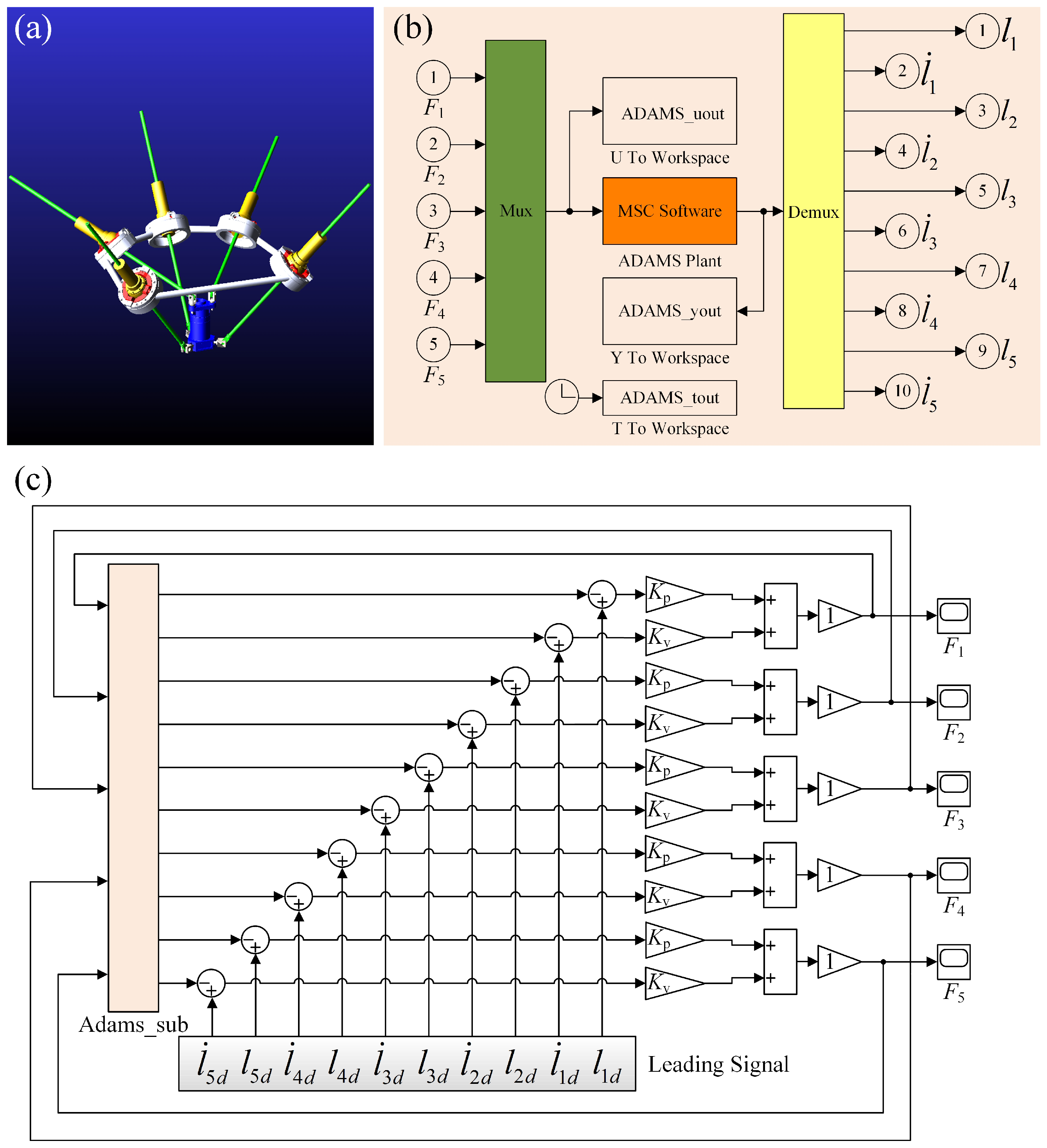
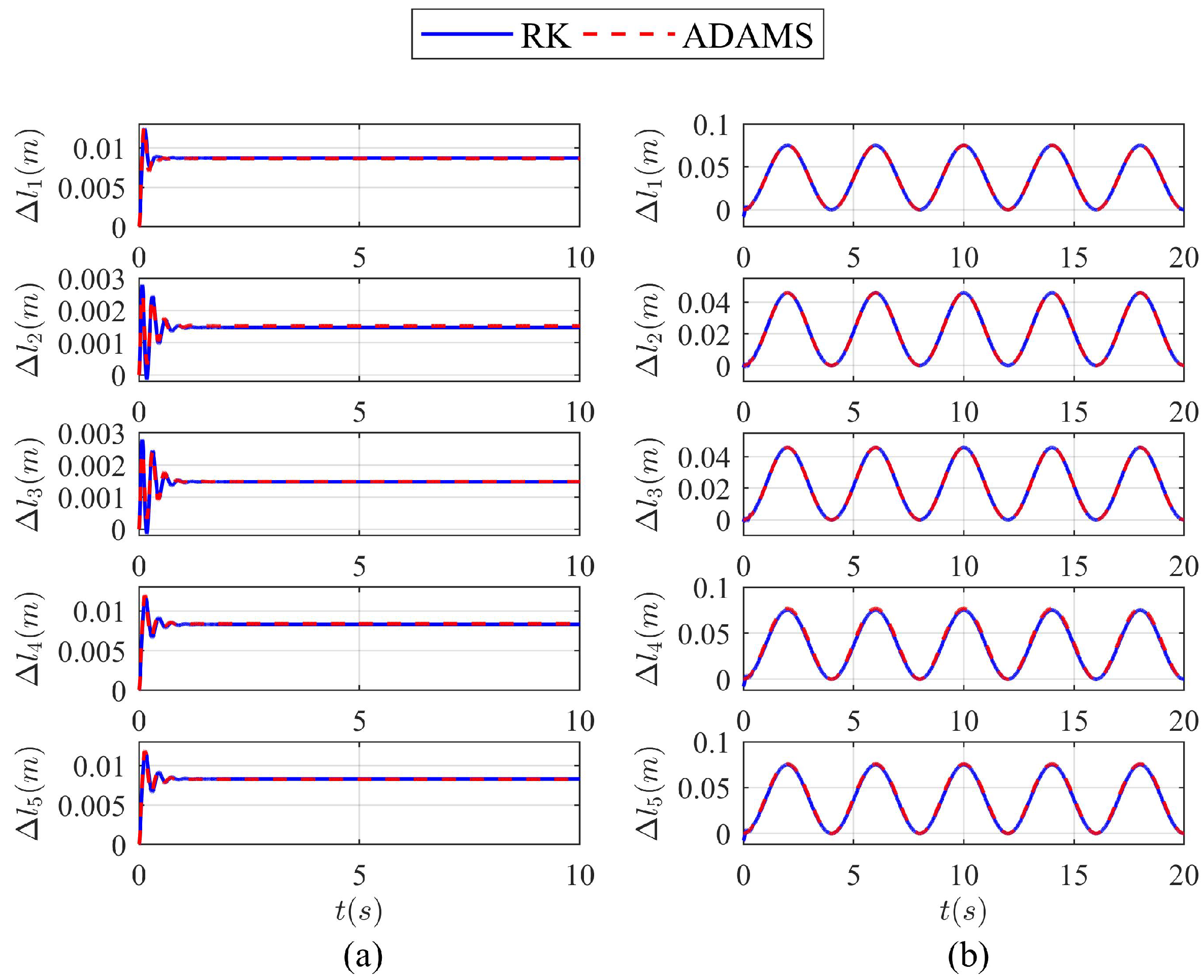
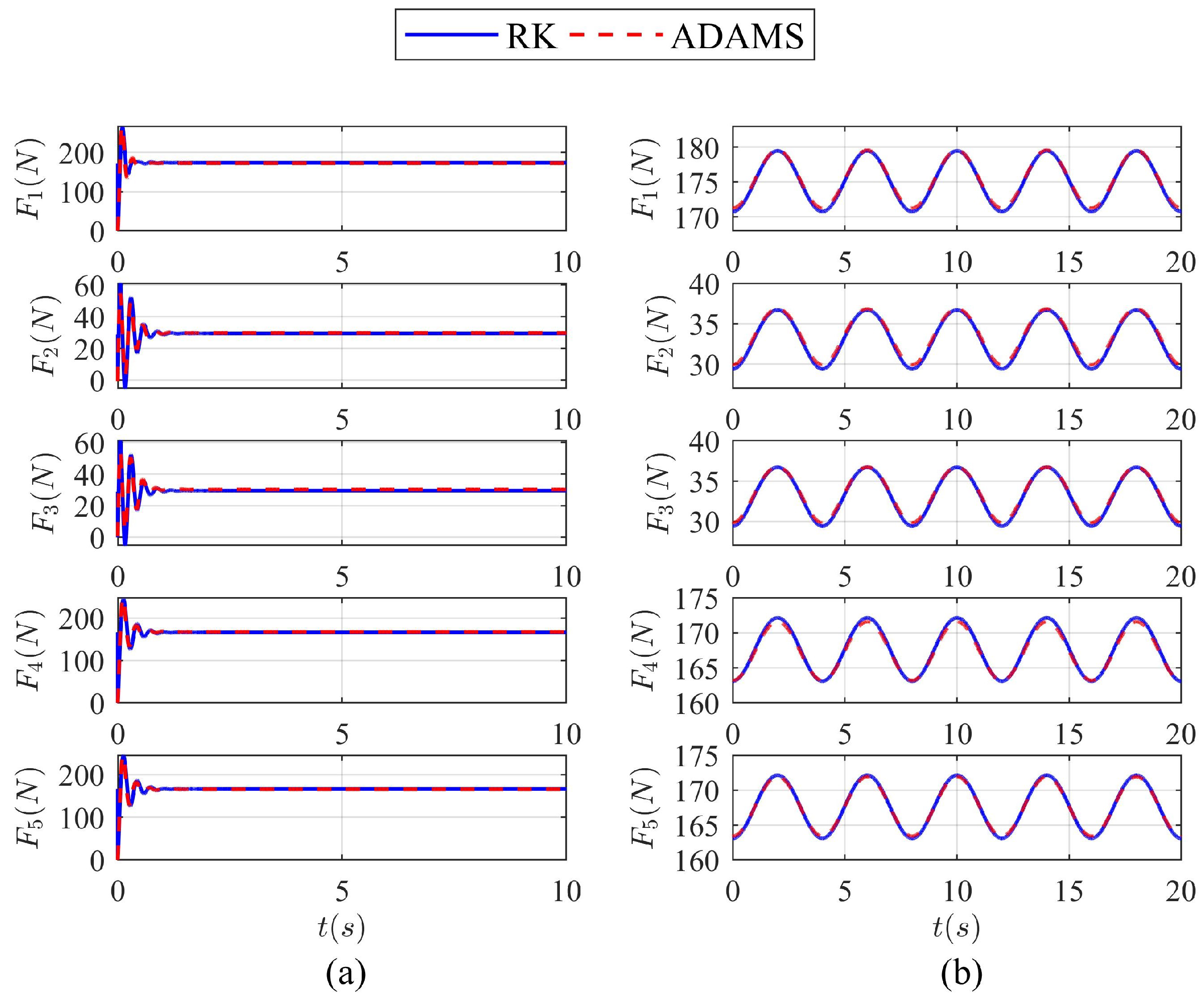
4. Dynamic Model Validation

As shown in the last section, the symbolic derivation of the established dynamic model of such 5-DoF spatial PM is complicated, implying the necessity of model validation. For this purpose, we assume that the spatial PM is under ideal actuation and not disturbed by external forces, and use the multi-body dynamics software MSC ADAMS to simulate the dynamic behavior of the spatial PM. The geometrical and physical parameters of the mechanism are given in Table 1.
The Runge–Kutta (RK) method with variable step size is employed to solve the forward dynamics of the model that we established in Section 3, and this method is abbreviated as the RK method. Meanwhile, we run the co-simulation by using MSC ADAMS and MATLAB/Simulink for the 5-DoF spatial PM, as sketched in Figure 3, in which the forward dynamics of the virtual prototype is obtained by ADAMS/Solve, and this method is abbreviated as ADAMS. In both ways of simulating forward dynamics, we implement the joint-based PD control with identical position gain and evaluate the performance of trajectory tracking of the end-effector. The joint-based PD control law with digital sampling is given by
F t = K p L d τ i L τ i + K v L ˙ d τ i L ˙ τ i ,
where L d and L ˙ d represent the desired position and velocity of limbs, respectively, and are generated by inverse kinematics of the spatial PM. The numerical solution based on the RK method and the co-simulation result is compared in Figure 4 and Figure 5, where the control frequency is fixed as 1000 Hz, or equivalently Δ τ = 0.001 s for Equation (32) and t τ i , τ i + 1 , K p = 20,000, K v = 400 .
As shown in Figure 5, the solution of Equation (32) obtained by the RK method is in agreement with that by the co-simulation, implying that the dynamic model represented by Equation (29) is reliable and therefore provides a basis for designing the model-based control, as will be discussed in next section.

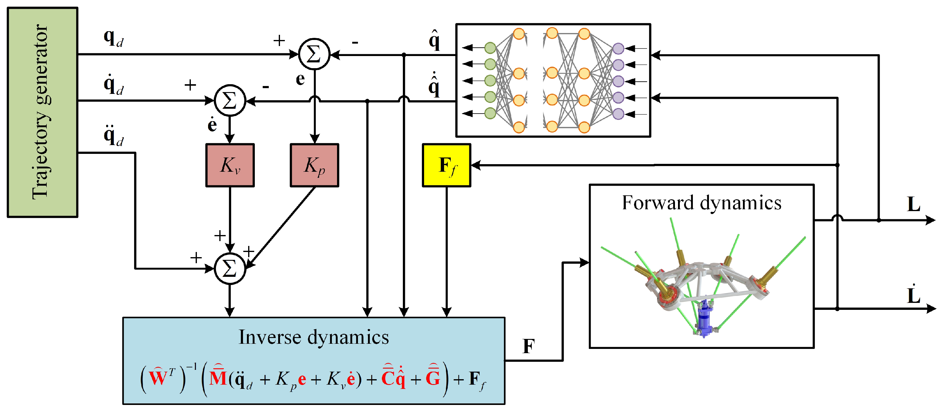
5. Control Design Based on Dynamic Model

The dynamic model provides a promising basis for designing feedback controllers with dynamic compensation, which has been proven effective in robot control with high precision. Given the dynamic model, the design of feedback control with dynamic compensation is routine for serial mechanisms. However, due to the difficulties in obtaining real-time state of the end-effectors of spatial PMs, dynamic models in the form of Equation (29) are incomplete to incorporate with a feedback controller with dynamic compensation, which requires direct measurement of the state of end-effector or alternatively an immediate calculation based on the state of actuators. Since the direct measurement is apt to be limited by the experimental devices as well as the working environment and the forward kinematics calculation is time-consuming in its traditional manner, we propose to predict the state of the end-effector of the 5-DoF spatial PM in terms of a neural network which is trained on inverse kinematics data. Then the proposed controller with feedback dynamic compensation is introduced and compared with the results of PD control as well as model-based control with feedforward dynamic compensation.

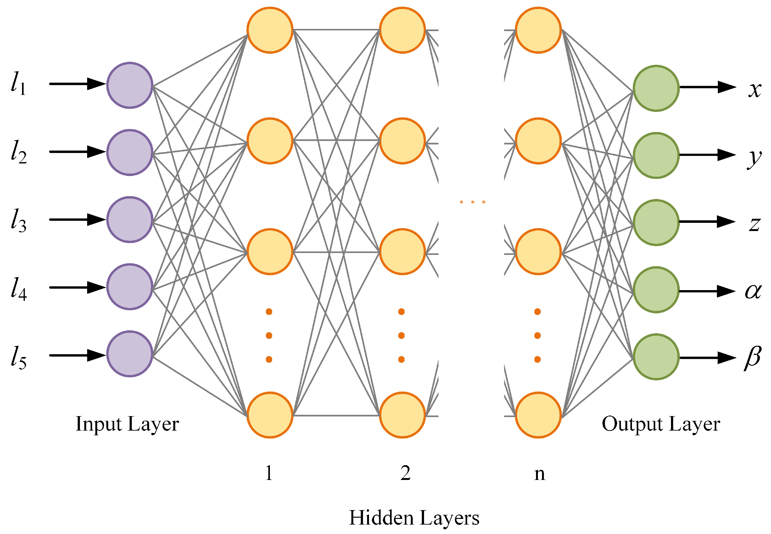
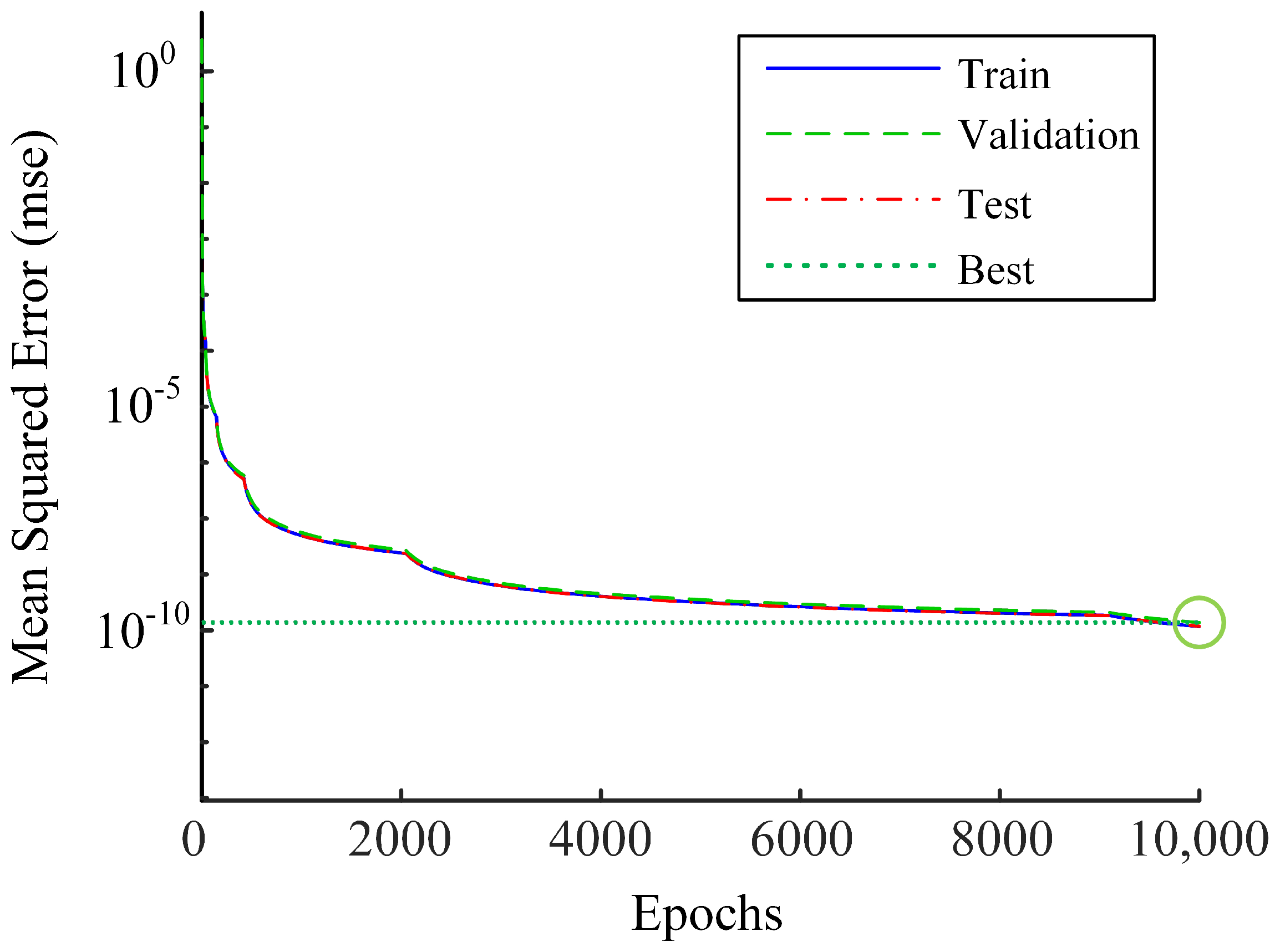
5.1. End-Effector State Predictor of Spatial PM Based on DNN Method

For the spatial PM of concern, the task of forward kinematics is to determine the position and orientation of end-effector, namely, q = x y z α β T for measured lengths of ball screws, i.e., l i ( i = 1 , 2 , 3 , 4 , 5 ) . Noting the complexity of the forward kinematics of the 5-DoF spatial PM, the deep neural network is invoked to fit the map from states of the end-effector to states of the actuators. To construct the training data for the DNN, 100,000 data points from the prescribed region in the task space of the end-effector (Table 2), viewed as the output of the DNN, are randomly generated and the corresponding lengths of ball screws, taken as the input of the DNN, are calculated through the inverse kinematics. According to the standard operation of training a DNN, all the data is normalized while 80% of it is treated as the training set, 10% as the test set, and the rest 10% as the validation set.
As shown in Figure 6, the DNN consists of three parts: the input layer, the hidden layers, and the output layer. With the increase in the number of hidden layers, the fitting capability of DNN is enhanced. However, too many hidden layers with excessively numerous parameters will lead to a complicated neural network which may suffer from overfitting during the offline training and computationally inefficiency during the online deployment [34]. To balance the performance of the network and the computational efficiency, we choose the number of hidden layers of DNN as 5, and the numbers of neurons in each hidden layer as 30, 30, 20, 20 and 20, respectively. The DNN is trained by using MATLAB Neural Network Toolbox, and Figure 7 shows the mean squared error (MSE) during the training process for the normalized input data. In order to show the performance of the DNN for the dimensional data, we construct another 10,000 sets of test data within the same region by using the aforementioned method and compare the data with the output of the DNN, as shown in Table 3.
To verify the effectiveness of the proposed DNN-based approximation of forward kinematics, we employ Newton’s method to carry out numerical simulations. It should be noted that the initial guess of each step of Newton’s method is chosen as the output of the previous step and therefore the convergence of iterations is speeded up. Meanwhile, the maximum permissible error is fixed as 1 × 10 5 (m), which ensures that Newton’s method has the same expected accuracy as the DNN (Table 3). Figure 8 shows the comparison of time-consuming forward kinematics calculation for spatial motion signals with different velocities within 10 s at a sampling frequency of 1000 Hz. The calculations are implemented on an Intel (R) Core (TM) i7-6700K CPU @ 4.00 GHz, with 16 GB RAM, and the average calculation time of the DNN method is less than 3 × 10 5 s. As shown in Figure 8, the number of iterations of Newton’s method increases as the speed of the tracking signal rises, while the computational efficiency of the DNN-based approximation of forward kinematics is not varied with the speed of the tracking signal. The above results indicate that the DNN method has superior performance in computational efficiency and therefore provides a promising basis for real-time control.

5.2. Design of the Controller with DNN Based Feedback Compensation

With the aid of the DNN-based end-effector state predictor, we can obtain the state of the end-effector in terms of the state of driving limbs in real-time, which makes it possible to realize the feedback compensation control of the 5-DoF spatial PM. As shown in Figure 9, the computed torque control with DNN-based feedback compensation can be expressed as
F = ( W T ) 1 ( M ¯ ( q ¨ d + K p e + K v e ˙ ) + C ¯ q ˙ + G ¯ ) + F f
In Equation (33), e = q d q ^ and e ˙ = q ˙ d q ^ ˙ denote, respectively, the tracking errors of position and velocity of the end-effector, where q d represents the leading signal (LS), and q ^ the prediction of q obtained by the DNN-based forward kinematics. M ¯ , C ¯ , G ¯ , and W represent the predictes of M ¯ , C ¯ , G ¯ , and W , respectively, and are generated by replacing q and q ˙ by their predicte in M ¯ , C ¯ , G ¯ , and W .
As a comparison, the control method using the feedforward signal for dynamic compensation in Ref. [22] is applied for the trajectory tracking control of the 5-DoF spatial PM. This controller compensates the system dynamics by the desired signal rather than the real-time state of the end-effector, therefore the dynamics compensation part of this controller is open-loop. The dynamic feedforward control is formulated as
F = ( W T ) 1 ( M ¯ q ¨ d + C ¯ q ˙ d + G ¯ ) + K p L ˜ + K v L ˜ ˙ + F f .
In Equation (34), L ˜ = L d L , L ˜ ˙ = L ˙ d L ˙ , and denote, respectively, the tracking errors of position and velocity of the driving limbs, where L d represents the desired position of the driving limbs. M ¯ , C ¯ , G ¯ , and W are the predictes of M ¯ , C ¯ , G ¯ , and W respectively, and are generated by replacing M ¯ , C ¯ , G ¯ , and W , espectively, and are generated by replacing q and q ˙ by q d and q ˙ d in M ¯ , C ¯ , G ¯ , and W .

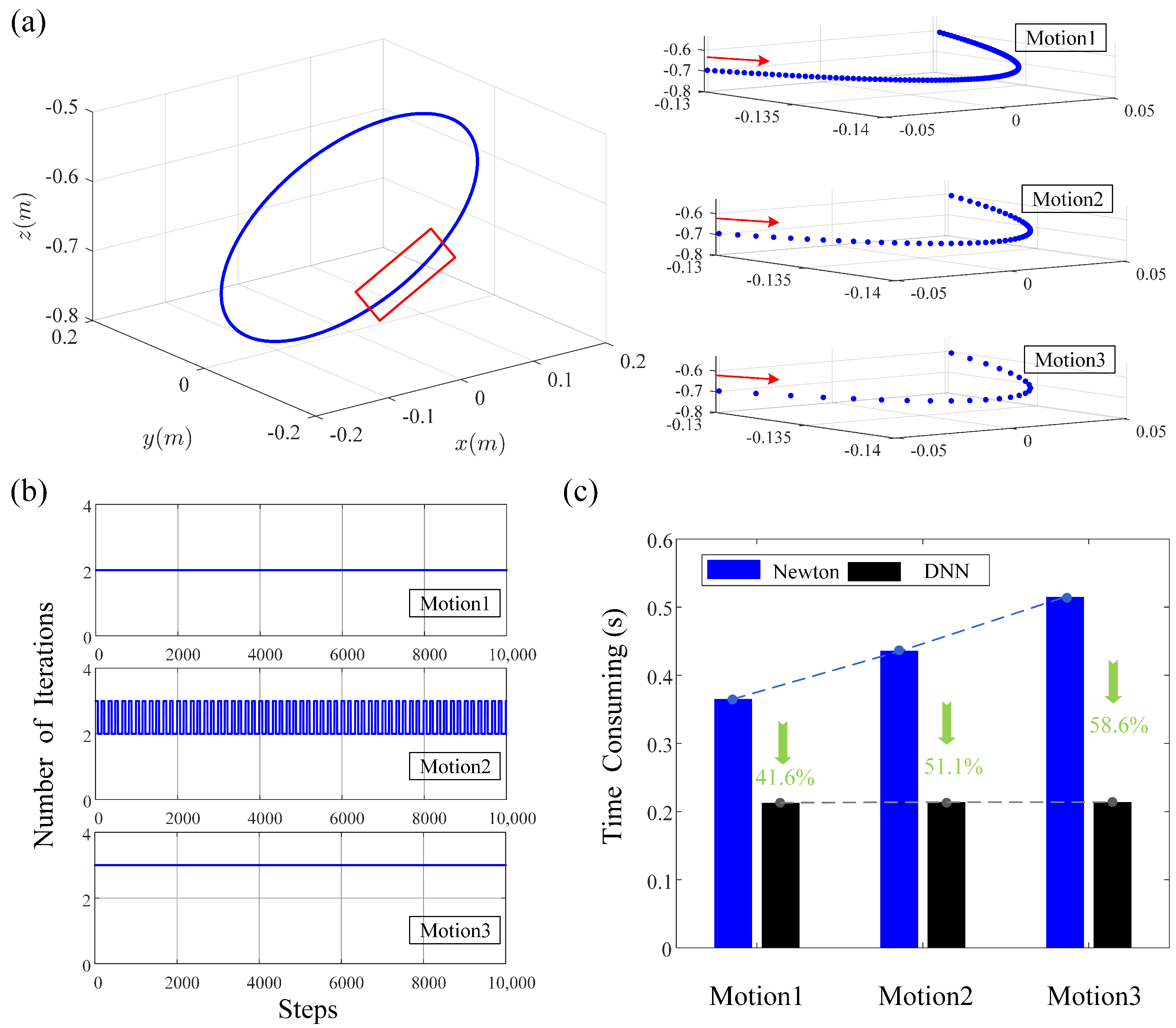
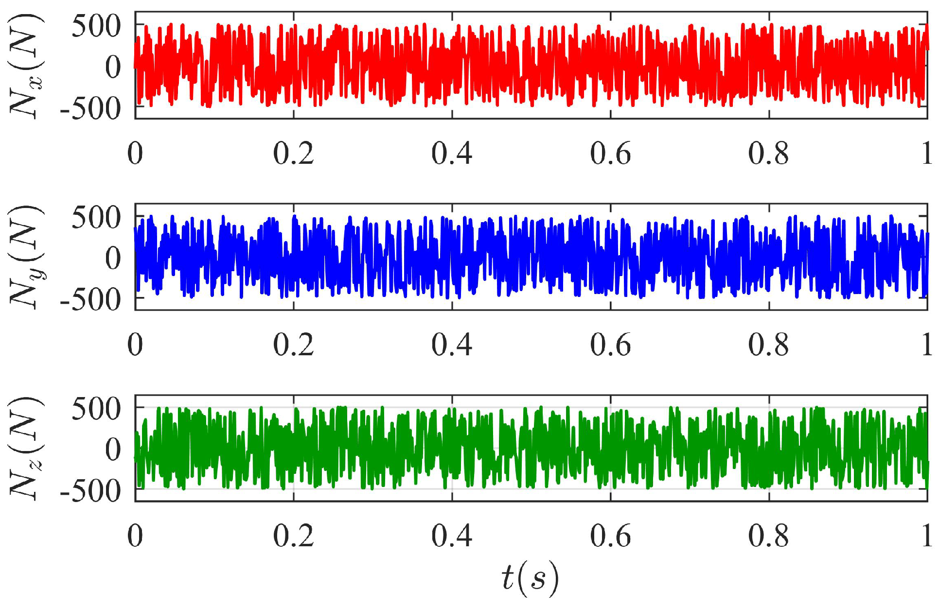
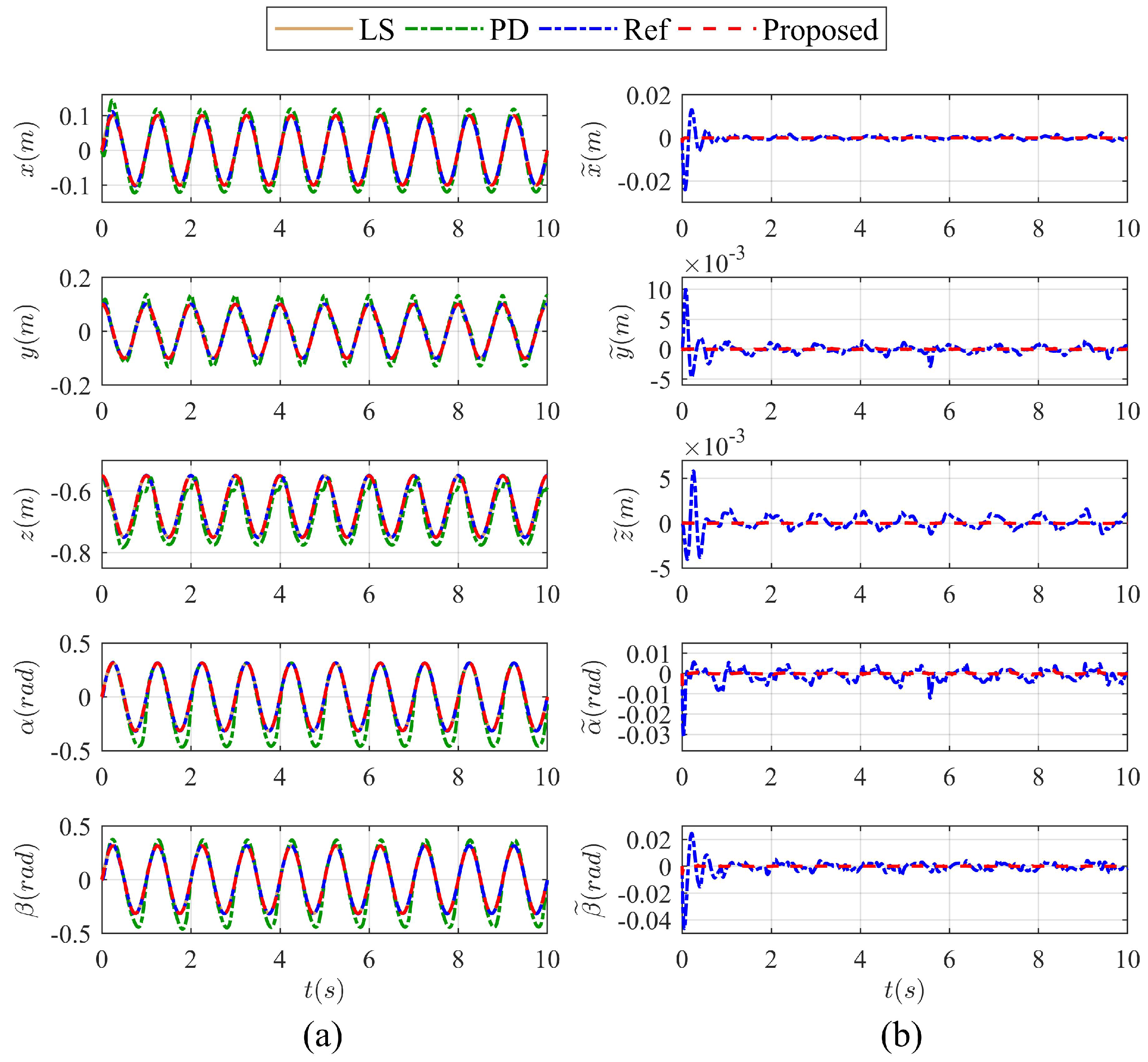
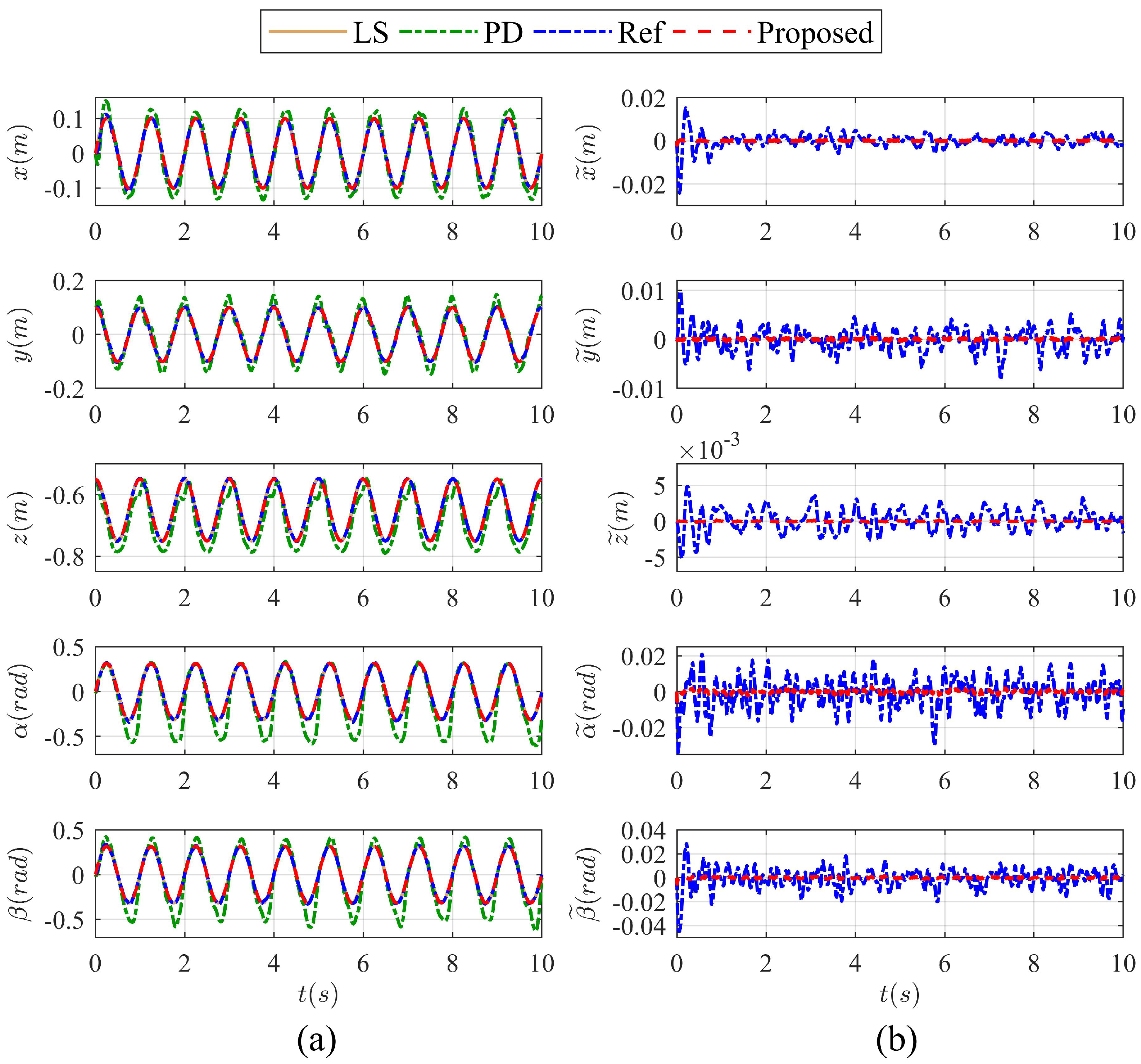
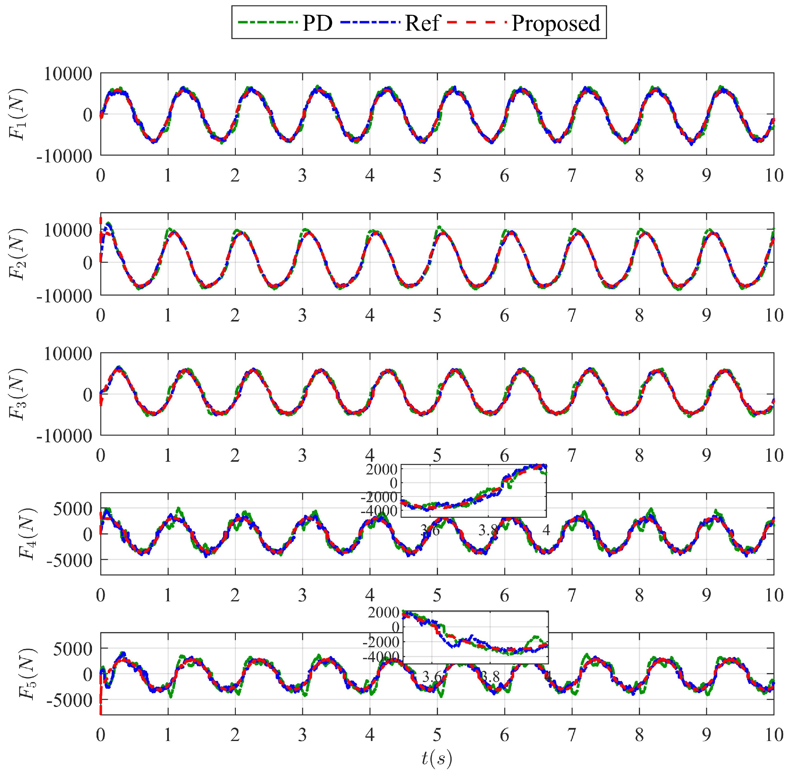
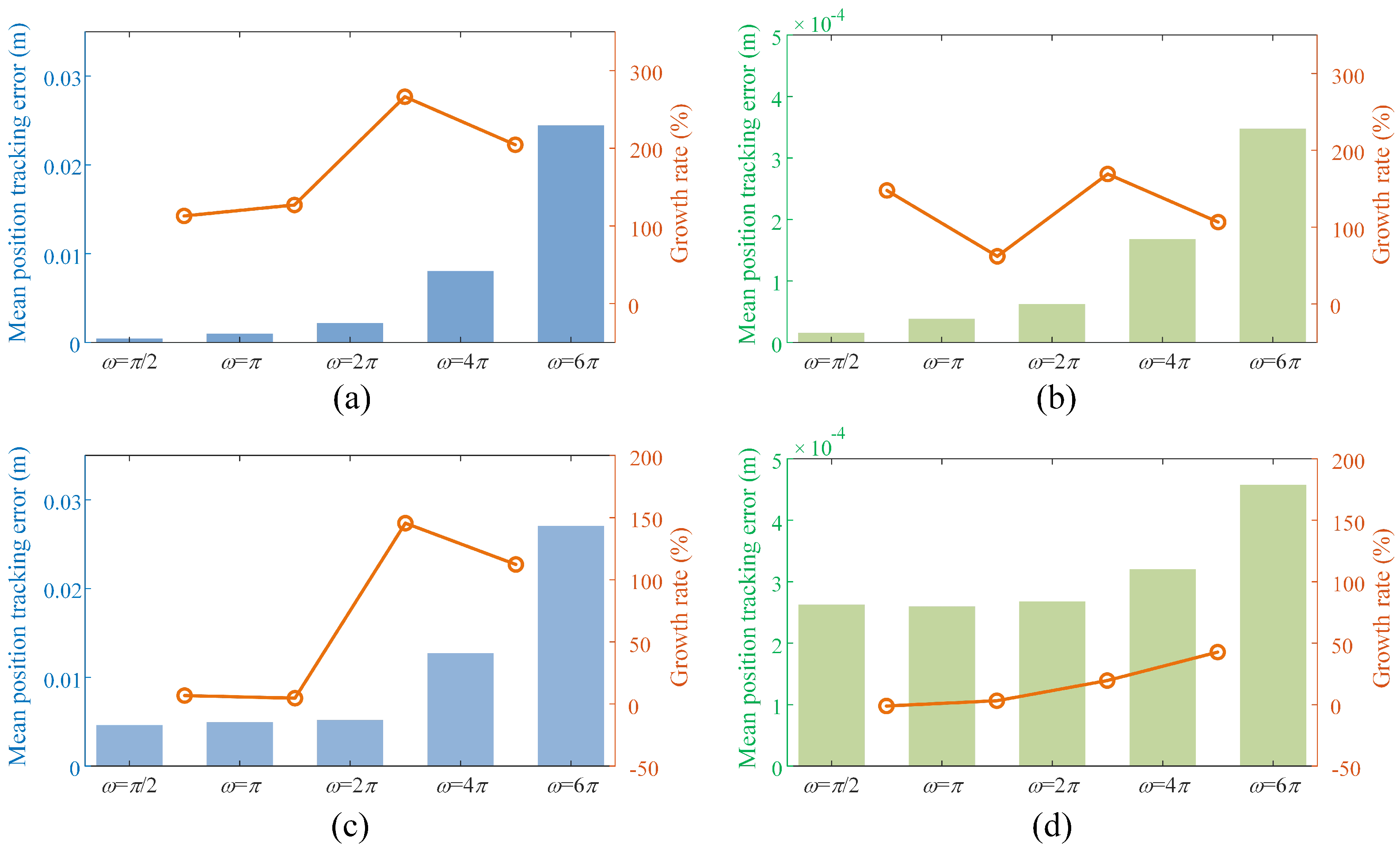
5.3. Numerical Results

Numerical simulations are carried out to verify the effectiveness of the proposed controller with DNN-based feedback compensation, while the joint-based PD control and the dynamic feedforward control in Ref. [22] are provided as comparisons. The tracking trajectory in the task space of the 5-DoF SPM is given as x = 0.1 sin ω t , y = 0.1 cos ω t , z = 0.65 + 0.1 cos ω t , α = π 10 sin ω t , β = π 10 sin ω t , where ω is chosen as 2 π . We discuss two cases of the tracking control problem with respect to the above signal: (1) only the friction in drive limbs is considered and the external disturbance is neglected and (2) the friction and the disturbance are both taken into account. For both cases, the parameters for three controllers are chosen as K p = 20 , 000 and K v = 400 . For cases 1 and 2, the friction model and parameters are consistent with the identification results of previous work [22]. In case 2, the external disturbance is mainly caused by the cutting forces on the mechanism performing the cutting task and is assumed to have the following form
N = rand 500 , 500 rand 500 , 500 rand 500 , 500 0 0 T .
The external disturbance in the three directions is shown in Figure 10.
For case 1, the tracking performance of the generalized coordinates of the 5-DoF spatial PM is presented in Figure 11. As shown in Figure 11a, two model-based controllers, i.e., the dynamic feedforward controller (Ref) and DNN-based feedback dynamic controller (proposed), can better track the leading signal (LS) than the model-free controller, i.e., the joint-based PD controller (PD). In Figure 11b, the tracking error of the proposed controller is consistently much smaller than that of the dynamic feedforward controller. For case 2, the findings consistent with the above are presented in Figure 12. With the addition of random external disturbances, the tracking performance of all three controllers decreases, while the proposed controller is still the most superior. Control forces under different controllers for case 2 are shown in Figure 13. The results show that the most severe jitter of control forces under PD control and the control forces of the proposed controller are smoother than that of the Ref controller as can be seen through the magnification window. Considering the universal existence of friction and disturbance in real applications, the above results have revealed the merit of the proposed controller with DNN-based feedback compensation as well as the necessity of dynamic modeling.
In addition, the performance of two model-based controllers tracking signals with different speeds is shown in Figure 14, where the speed improvement of the trajectory is achieved increasing the value of ω . The results show that the mean position tracking error of the proposed controller is much smaller than that of the dynamic feedforward controller when tracking signals with different speeds, and the proposed controller also has a lower error growth rate than the dynamic feedforward controller at high speed.

6. Conclusions

This paper aims at providing a promising dynamic model for the accurate control of a particular prototype of a machining platform, namely, the 5-DoF spatial PM. Choosing the position and orientation of the end-effector as the generalized coordinates, the kinetic energy and potential energy are formulated based on the inverse kinematics, and consequently, the dynamic model is established by using the Lagrangian method. The numerical solution of the dynamic model agrees well with the output of co-simulation by using MSC ADAMS and MATLAB/Simulink, verifying the modeling process.
In order to improve the control performance, we implement the model-based controller with the feedback dynamic compensation, which is dependent on the forward kinematics of the mechanism. Considering the complexity of the forward kinematics of the 5-DoF spatial PM, the pre-trained DNN is introduced to predict the real-time state of the end-effector. The test results show that the DNN method offers a faster response than Newton’s method during the control in real-time, as well as ensuring prediction accuracy. On this basis, we design the computed torque control with DNN-based feedback compensation. The simulations show that, in the most complicated case that involves friction and external disturbance, the proposed controller with DNN-based feedback compensation outperforms the joint-based PD controller and the dynamic feedforward controller. In the cases of tracking trajectories with different speeds, the proposed controller also shows promising performance. These results indicate that the combination of the dynamic model and the DNN-based end-effector state predictor can provide a solid basis for the control with high precision.
It is worth noting that the deformation of driving limbs is ignored in this paper. Given the slender configuration of the driving limbs, their deformation may not be negligible for some specific cases. Therefore, building a more refined dynamic model of the 5-DoF spatial PM to address the flexible characteristic of the mechanism, and deploying the proposed control algorithm to the experimental prototype will be the aim of our future work.

Author Contributions

Conceptualization, D.G. and S.Z.; methodology, D.G. and Z.X.; software, D.G. and Z.X.; validation, D.G. and S.Z.; formal analysis, D.G., X.S. and Z.X.; data curation, D.G.; writing—original draft preparation, D.G. and S.Z.; writing—review and editing, D.G. and S.Z.; supervision, S.Z.; project administration, X.S. and S.Z.; funding acquisition, X.S. and S.Z. All authors have read and agreed to the published version of the manuscript.

Funding

This work was supported by the National Natural Science Foundation of China (Grant Nos. 91748205, 12072237, 11872277, and 12122208) and the Fundamental Research Funds for the Central Universities under Grant No. 22120220590.

Data Availability Statement

Data are available upon request from the authors.

Conflicts of Interest

The authors declare no conflict of interest.

Appendix A. The Detailed Expressions of Position of the Key Points

In : o x y z , the coordinates of B i ( i = 1 , 2 , 3 , 4 , 5 ) can be written as
B j = R 1 cos a R 1 sin a 0 T , B 4 = R 1 cos 3 π 4 R 1 sin 3 π 4 0 T , B 5 = R 1 cos π 4 R 1 sin π 4 0 T ,
where a = 2 π j 3 π 6 , and j = 1 , 2 , 3 . In : o x y z , the coordinates of points P i ( i = 1 , 2 , , 5 ) can be written as
P j = R 2 cos a R 2 sin a 0 T , P k = R 2 cos b R 2 sin b H T ,
where b = sin 2 π k 2 3 π 6 , and k = 4 , 5 .

Appendix B. Proof of Equation (25)

The relationship between Q c and Q is as follows:
Q c T δ q c = Q T δ q .
Together with δ q c = q c q δ q , we have
Q c T q c q Q T δ q = 0 .
Since δ q is free to vary, Equation (A4) can be rewritten as
Q c T q c q Q T = Q c T S Q T = 0 .
According to Equation (A5), we have
Q = S T Q c .
Similarly, the relationship between the axial force F = F 1 F 2 F 3 F 4 F 5 T and the generalized force is as follows:
F T δ L = Q T δ q .
From δ L = L q δ q , we obtain
F T L q Q T δ q = 0 .
Since δ q can be arbitrary, Equation (A8) can be rewritten as
F T L q Q T = F T W Q T = 0 .
According to Equation (A9), we have
Q = W T F .
Finally, it is apparent that combining Equation (A6) and Equation (A10) yields Equation (25).

Appendix C. Symbolic Derivation of the Dynamic Equation

In this appendix, the pseudocodes of the symbolic derivation are collected. The inertial matrix ( M q c 6 × 6 ) is computed using Algorithm A1
Algorithm A1: The symbolic derivation of the inertial matrix
S 1 :
Declare the types of all the variables and initialize them.
S 2 :
Define the vectors of the end-effector: q c = x y z α β γ T and q ˙ c = x ˙ y ˙ z ˙ α ˙ β ˙ γ ˙ T .
S 3 :
Input the geometric, inertial and other time independent parameters.
S 4 :
Compute the rotation matrix R ( α , β , γ ) (Equation (1)), the vector L (Equation (6)), and the Jacobian matrix W (Equation (13)).
S 5 :
Compute the velocity vectors and matrices: ω p (Equation (9)), ω i ( i = 1 , 2 , , 5 ) (Equation (11)), and L ˙ (Equation (14)).
S 6 :
Compute the total kinetic energy of the mechanism: T (Equations (16)–(20)).
      for  i = 1 to 6 do
    for  j = 1 to 6 do
      S 7 : Compute M i , j = 2 T q c i q c j
    end
 end
According to the Lagrange equation, the Coriolis matrix ( C q c , q ˙ c 6 × 6 ) and the gravitational terms ( G q c 6 × 1 ) are computed using the following Algorithm A2.
Algorithm A2: The symbolic derivation of the Coriolis matrix and gravitational terms
S 1 :
Define C q c , q ˙ c 6 × 6 = 0 6 × 6 .
S 2 :
Compute the total potential energy (V) of the mechanism (Equations (21)–(23)).
      for  i = 1 to 6 do
    for  j = 1 to 6 do
      for  k = 1 to 6 do
      S 3 : Compute C i , j = C i , j + M i , j q c k 1 2 M j , k q c i q ˙ c k .
      end
    end
  S 4 : Compute G i = V q c i .
 end

References

  1. Liu, X.; Yao, J.; Xu, Y.; Zhao, Y. Research of driving force coordination mechanism in parallel manipulator with actuation redundancy and its performance evaluation. Nonlinear Dyn. 2017, 90, 983–998. [Google Scholar] [CrossRef]
  2. Luo, X.; Xie, F.; Liu, X.J.; Xie, Z. Kinematic calibration of a 5-axis parallel machining robot based on dimensionless error mapping matrix. Robot. Comput.-Integr. Manuf. 2021, 70, 102115. [Google Scholar] [CrossRef]
  3. Liu, X.J.; Bi, W.Y.; Xie, F.G. An energy efficiency evaluation method for parallel robots based on the kinetic energy change rate. Sci. China Technol. Sci. 2019, 62, 1035–1044. [Google Scholar] [CrossRef]
  4. Liu, X.J.; Bi, W.Y.; Xie, F.G. DELTA: A simple and efficient parallel robot. Robotica 1990, 8, 105–109. [Google Scholar]
  5. Hao, Q.; Guan, L.; Wang, J.; Wang, L. Dynamic feedforward control of a novel 3-PSP 3-DoF parallel manipulator. Chin. J. Mech. Eng. 1990, 24, 676. [Google Scholar] [CrossRef]
  6. Xin, G.; Deng, H.; Zhong, G. Closed-form dynamics of a 3-DoF spatial parallel manipulator by combining the Lagrangian formulation with the virtual work principle. Nonlinear Dyn. 2016, 86, 1329–1347. [Google Scholar] [CrossRef]
  7. Zhao, C.; Chen, Z.; Song, J.; Wang, X.; Ding, H. Deformation analysis of a novel 3-DoF parallel spindle head in gravitational field. Mech. Mach. Theory 2020, 154, 104036. [Google Scholar] [CrossRef]
  8. Abadi, B.N.R.; Farid, M.; Mahzoon, M. Redundancy resolution and control of a novel spatial parallel mechanism with kinematic redundancy. Mech. Mach. Theory 2019, 133, 112–126. [Google Scholar] [CrossRef]
  9. Ebrahimi, I.; Carretero, J.A.; Boudreau, R. 3-PRRR redundant planar parallel manipulator: Inverse displacement, workspace and singularity analyses. Mech. Mach. Theory 2007, 42, 1007–1016. [Google Scholar] [CrossRef]
  10. Muralidharan, V.; Bose, A.; Chatra, K.B.; Yopadhyay, S. Methods for dimensional design of parallel manipulators for optimal dynamic performance over a given safe working zone. Mech. Mach. Theory 2020, 147, 103721. [Google Scholar] [CrossRef]
  11. Xie, Z.; Xie, F.; Liu, X.J.; Wang, J.; Shen, X. Parameter optimization for the driving system of a 5 degrees-of-freedom parallel machining robot with planar kinematic chains. J. Mech. Robot. 2019, 11, 041003. [Google Scholar] [CrossRef]
  12. Azar, A.T.; Zhu, Q.; Khamis, A.; Zhao, D. Control design approaches for parallel robot manipulators: A review. Int. J. Model. Identif. Control 2017, 28, 199–211. [Google Scholar] [CrossRef]
  13. Mei, B.; Xie, F.; Liu, X.J.; Yang, C. Elasto-geometrical error modeling and compensation of a five-axis parallel machining robot. Int. J. Model. Identif. Control 2021, 69, 48–61. [Google Scholar] [CrossRef]
  14. Wu, J.; Wang, J.; Wang, L.; Li, T. Dynamics and control of a planar 3-DoF parallel manipulator with actuation redundancy. Mech. Mach. Theory 2009, 44, 835–849. [Google Scholar] [CrossRef]
  15. Huang, G.; Zhang, D.; Tang, H.; Kong, L.; Song, S. Analysis and control for a new reconfigurable parallel mechanism. Int. J. Adv. Robot. Syst. 2020, 17, 149–167. [Google Scholar] [CrossRef]
  16. Niu, X.; Yang, C.; Tian, B.; Li, X.; Han, J.; Agrawal, S.K. Modal decoupled dynamics-velocity feed-forward motion control of multi-DoF robotic spine brace. IEEE Access 2018, 6, 65286–65297. [Google Scholar] [CrossRef]
  17. Yang, C.; Huang, Q.; Jiang, H.; Peter, O.O.; Han, J. PD control with gravity compensation for hydraulic 6-DoF parallel manipulator. Mech. Mach. Theory 2010, 45, 666–677. [Google Scholar] [CrossRef]
  18. Chen, Z.; Xu, L.; Zhang, W.; Li, Q. Closed-form dynamic modeling and performance analysis of an over-constrained 2PUR-PSR parallel manipulator with parasitic motions. Nonlinear Dyn. 2019, 96, 517–534. [Google Scholar] [CrossRef]
  19. Zi, B.; Wang, N.; Qian, S.; Bao, K. Design, stiffness analysis and experimental study of a cable-driven parallel 3D printer. Mech. Mach. Theory 2019, 132, 207–222. [Google Scholar] [CrossRef]
  20. Chai, X.; Wang, M.; Xu, L.; Ye, W. Dynamic modeling and analysis of a 2PRU-UPR parallel robot based on screw theory. IEEE Access 2020, 8, 78868–78878. [Google Scholar] [CrossRef]
  21. Yang, C.; Han, J.; Zheng, S.; Ogbobe Peter, O. Dynamic modeling and computational efficiency analysis for a spatial 6-DoF parallel motion system. Nonlinear Dyn. 2012, 67, 1007–1022. [Google Scholar] [CrossRef]
  22. Xie, Z.; Xie, F.; Liu, X.J.; Wang, J.; Mei, B. Tracking error prediction informed motion control of a parallel machine tool for high-performance machining. Int. J. Mach. Tools Manuf. 2021, 164, 103714. [Google Scholar] [CrossRef]
  23. Abdellatif, H.; Heimann, B. Advanced model-based control of a 6-DoF hexapod robot: A case study. IEEE/ASME Trans. Mechatronics 2009, 15, 269–279. [Google Scholar] [CrossRef]
  24. Antonov, A.; Fomin, A.; Glazunov, V.; Kiselev, S.; Carbone, G. Inverse and forward kinematics and workspace analysis of a novel 5-DoF (3T2R) parallel–serial (hybrid) manipulator. Int. J. Adv. Robot. Syst. 2021, 18, 1729881421992963. [Google Scholar] [CrossRef]
  25. Sun, T.; Yang, S. An approach to formulate the Hessian matrix for dynamic control of parallel robots. IEEE/ASME Trans. Mechatron. 2019, 24, 271–281. [Google Scholar] [CrossRef]
  26. Zubizarreta, A.; Cabanes, I.; Marcos, M.; Pinto, C. A redundant dynamic model of parallel robots for model-based control. Robotica 2013, 31, 203–216. [Google Scholar] [CrossRef]
  27. Nanua, P.; Waldron, K.J.; Murthy, V. Direct kinematic solution of a Stewart platform. IEEE Trans. Robot. Autom. 1990, 6, 438–444. [Google Scholar] [CrossRef]
  28. Choi, H.B.; Konno, A.; Uchiyama, M. Closed-form forward kinematics solutions of a 4-DoF parallel robot. Int. J. Control Autom. Syst. 2009, 7, 858–864. [Google Scholar] [CrossRef]
  29. Nouri, R.; Abadi, B.; Carretero, J.A. Modeling and Real-Time Motion Planning of a Class of Kinematically Redundant Parallel Mechanisms With Reconfigurable Platform. J. Mech. Robot. 2023, 15, 021004. [Google Scholar] [CrossRef]
  30. Zhang, D.; Lei, J. Kinematic analysis of a novel 3-DoF actuation redundant parallel manipulator using artificial intelligence approach. Robot. Comput.-Integr. Manuf. 2011, 27, 157–163. [Google Scholar] [CrossRef]
  31. Parikh, P.J.; Lam, S.S. Solving the forward kinematics problem in parallel manipulators using an iterative artificial neural network strategy. Int. J. Adv. Manuf. Technol. 2009, 40, 595–606. [Google Scholar] [CrossRef]
  32. Xie, F.; Liu, X.J.; Wang, J.; Wabner, M. Kinematic optimization of a five degrees-of-freedom spatial parallel mechanism with large orientational workspace. J. Mech. Robot. 2017, 9, 051005. [Google Scholar] [CrossRef]
  33. Xie, F.; Liu, X.J.; Luo, X.; Wabner, M. Mobility, singularity, and kinematics analyses of a novel spatial parallel mechanism. J. Mech. Robot. 2016, 8, 061022. [Google Scholar] [CrossRef]
  34. Hagiwara, K.; Fukumizu, K. Relation between weight size and degree of over-fitting in neural network regression. Neural Netw. 2008, 21, 48–58. [Google Scholar] [CrossRef] [PubMed]
Figure 1. Geometric model of the proposed spatial PM with 5-DoF: (a) CAD model and (b) kinematic scheme.
Machines 11 00195 g001
Figure 3. Diagram of co-simulation by using MSC ADAMS and MATLAB/Simulink. (a) virtual prototype of 5-DoF spatial PM in ADAMS. (b) 5-DoF spatial PM as an ADAMS plant in MATLAB/Simulink. (c) Block diagram of co-simulation with PD control in Simulink, where ADAMS_sub represents the ADAMS plant, and K p , K v represent the position gain and velocity gain, respectively.
Machines 11 00195 g003
Figure 4. Comparison of the variations of L l 1 , l 2 , l 3 , l 4 , l 5 under RK method and ADAMS. (a) Time history plot of the variations of L l 1 , l 2 , l 3 , l 4 , l 5 under the positioning motion, and the tracking signal of the end-effector is given as x = 0 , y = 0 , z = 0.55 , α = 0 , and β = 0 . (b) Time history plot of the variations of L l 1 , l 2 , l 3 , l 4 , l 5 under the periodic motion, and the tracking signal of the end-effector is given as x = 0 , y = 0 , z = 0.6 + 0.05 sin π 2 t , α = 0 , and β = 0 .
Machines 11 00195 g004
Figure 5. Comparison of the evolution of the axial forces obtained by RK method and ADAMS. (a) Time history plot of five axial forces under the positioning motion and (b) Time history plot of five axial forces under the periodic motion.
Machines 11 00195 g005
Figure 6. The structure of the Deep Neural Network.
Machines 11 00195 g006
Figure 7. Training performance of the DNN model.
Machines 11 00195 g007
Figure 8. Comparison of time-consuming between the DNN-based method and Newton’s method of forward kinematics calculation for spatial motion signals with different velocities: (a) the spatial motion signal: x = 0.14 sin ω t , y = 0.14 cos ω t , z = 0.65 + 0.12 cos ω t , α = 0 , β = 0 , where ω is 2 π , 6 π , and 10 π in cases of motion1, motion2, and motion3, respectively; (b) number of iterations of Newton’s method in different motions; (c) time consuming of forward kinematics calculation.
Machines 11 00195 g008
Figure 9. Block diagram of the proposed controller with DNN-based feedback compensation.
Machines 11 00195 g009
Figure 10. The external disturbance signals during 0–1 s.
Machines 11 00195 g010
Figure 11. Tracking performance of the generalized coordinates of the 5-DoF spatial PM for case 1: (a) comparison of trajectory tracking with different controllers and (b) comparison of tracking error between the dynamic feedforward controller and proposed controller.
Machines 11 00195 g011
Figure 12. Tracking performance of the generalized coordinates of the 5-DoF spatial PM for case 2: (a) comparison of trajectory tracking with different controllers and (b) comparison of tracking error between the dynamic feedforward controller and proposed controller.
Machines 11 00195 g012
Figure 13. Control forces under different controllers for case 2.
Machines 11 00195 g013
Figure 14. Mean position tracking error and error growth rate of two model-based controllers tracking signals with different speeds: (a) the dynamic feedforward controller in case 1, (b) the proposed controller in case 1, (c) the dynamic feedforward controller in case 2, and (d) the proposed controller in case 2.
Machines 11 00195 g014
Table 1. The geometrical parameters and the physical parameters of the mechanism.
Geometrical ParameterValuePhysical ParameterValue
l t o t a l 1.500 (m) m 1 34.443 (kg)
H0.300 (m) m 2 5.756 (kg)
R 1 0.600 (m) m 3 15.000 (kg)
R 2 0.065 (m) J c 1 0.145 ( kg · m 2 )
e 1 0.063 (m) J c 2 1.079 ( kg · m 2 )
e 2 0.750 (m) I x x 0.419 ( kg · m 2 )
// I y y 0.088 ( kg · m 2 )
// I z z 0.419 ( kg · m 2 )
Table 2. Motion range of the end-effector in training data set.
DescriptionRange
Range of x ( mm ) 150 , 150
Range of y ( mm ) 150 , 150
Range of z ( mm ) 800 , 500
Range of α ( rad ) π π 9 9 , π π 9 9
Range of β ( rad ) π π 9 9 , π π 9 9
Table 3. The performances of the DNN after training on the dimensional test data set.
SymbolMaximum ErrorMSE
x(m) 3.04 × 10 6 3.84 × 10 13
y(m) 3.50 × 10 6 3.32 × 10 13
z(m) 4.82 × 10 6 7.05 × 10 13
α (rad) 1.32 × 10 5 5.06 × 10 12
β (rad) 2.62 × 10 5 8.41 × 10 12
L (m) 6.98 × 10 6 3.33 × 10 12
Disclaimer/Publisher’s Note: The statements, opinions and data contained in all publications are solely those of the individual author(s) and contributor(s) and not of MDPI and/or the editor(s). MDPI and/or the editor(s) disclaim responsibility for any injury to people or property resulting from any ideas, methods, instructions or products referred to in the content.

