1. Introduction
Due to the high stiffness, large workspace/footprint ratio, and desirable dynamic characteristics, hybrid robots have been widely used in modern high-end equipment manufacturing fields such as aerospace, military, and rail transit [
1,
2,
3]. Pose accuracy is the most important index to evaluate the machining performance of hybrid robots. On the premise of guaranteeing good repeatability through manufacturing and assembly, calibration is an effective way to improve the robot pose accuracy [
4,
5,
6,
7].
Model-based calibration, also named kinematic calibration, is a classical technique widely used in engineering applications. It usually consists of four steps: modeling, measurement, identification, and compensation. The core step is to establish an error model that satisfies the requirements of continuity, completeness, and minimization [
8,
9]. However, a robot has many error sources, including not only geometric errors such as assembly and manufacturing errors [
10], but also many non-geometric errors such as friction, backlash, thermal deformation, and flexible deformation [
11]. Moreover, the study [
12] has shown that almost 20% of robot errors are caused by error sources that vary with the robot configurations, such as straightness errors in moving pairs and pitch errors. Hence, establishing a complete model that considers all error sources seems to be an impossible challenge.
The limitation of model-based calibration incentivizes the application of data-driven methodologies [
13], which estimate errors with an arbitrary posture using pre-measured errors at certain locations by curve fitting [
14], spatial interpolation [
15,
16,
17], and artificial neural networks (ANNs) [
18,
19,
20]. Then, compensation is conducted based on the estimated values [
21]. It usually involves three steps: measurement, estimation, and compensation. Along this track, Alici et al. proposed an approach to estimate the robot position errors using ordinary polynomials [
22] and Fourier polynomials [
23]. Bai et al. presented fuzzy interpolation to estimate the position errors using the pre-measured errors on cubic lattices [
24]. According to the spatial similarity of position errors, Tian et al. [
25] introduced an inverse distance weighting (IDW) method. Cai et al. [
26] utilized the kriging algorithm to approximate the robot error surface. Analogously, ANNs, such as extreme learning machine (ELM) [
27], back-propagation neural network (BPNN) [
28,
29], and radial basis function neural network (RBFNN) [
30] have been gradually applied in data-driven calibration. Although the data-driven method seems to be a promising approach due to its excellent prediction performance, it still cannot ignore the limitations in measurement and compensation, which seriously restricts its further development and application.
Data-driven calibration can theoretically compensate for all errors in the robot system. However, its compensation accuracy relies on massive measurement data. The study [
31] has shown that a few sampling configurations cannot accurately describe the robot error distribution, leading to poor accuracy after calibration, and the accuracy of some configurations may be even worse than that before calibration. It is worth mentioning that the measurement task always takes up the most of time in the calibration. Especially for robots with high-dimensional joint space, the sampling data required for accurate calibration exponentially increase with increasing dimensions of the joint space, leading to the curse of dimensionality [
32]. Consequently, the measurement task might take several days. The limitation of low measurement efficiency is an urgent problem to be solved in data-driven calibration.
Due to the limitation of the openness of the robot system and the difficulty in solving the analytic inverse kinematics, indirect approaches [
33] that modify the joint input or Cartesian coordinates are widely used in error compensation. Chen et al. [
34,
35] directly took the estimated error
(the deviation between the measured pose
and the desired pose
; i.e.,
) as the compensation value and assumed that commanding a robot to move to the Cartesian position
would cause it to reach
in reality; i.e.,
. However, the robot will actually reach a new pose,
, which involves an error
of another pose
, where in the general case
. To acquire the optimal compensation value, Zhao et al. proposed a series of iterative algorithms based on the kinematics [
36], Jacobian [
37], and optimization algorithms such as particle swarm optimization (PSO) [
38] and genetic algorithm (GA) [
39]. Although the compensation accuracy can be guaranteed to a certain extent, these approaches are not feasible for online compensation because of the high computational burden. In addition, the compensation approaches mentioned above are carried out based on the estimated errors, which inevitably introduce estimation residuals. More importantly, the cumbersome calibration process of prediction and compensation is very time-consuming, preventing this approach from being used in field applications.
Aiming to resolve these problems, a new calibration method has been proposed in research [
40], which could effectively solve the contradiction between calibration accuracy and measurement efficiency, as well as the problem of real-time error compensation. However, it still has some shortcomings in practical application, as described in detail in
Section 3.1 and
Section 4.1. Thus, an improved data-driven methodology is investigated in this paper. The significance lies in the improvement of measurement efficiency and practicality. In the measurement, an arbitrary motion of the robot is equivalently decomposed into three independent sub-motions. Next, the sub-motions are combined according to specific motion rules. In this manner, a large number of robot poses can be acquired in the whole workspace via a limited number of measurements, which effectively solves the curse of dimensionality in measurement. In compensation, the mapping between the nominal joint variables and joint compensation values is established based on a BPNN, which is trained directly using the measurement data through a unique training algorithm involving the robot inverse kinematics. Thus, the practicability of the data-driven methodology is greatly improved.
The paper is organized as follows.
Section 2 is the system description of the six degrees of freedom (DOF) hybrid robot.
Section 3 introduces the principle of motion decomposition and the implementation process of decomposition measurement.
Section 4 illustrates an improved data-driven calibration methodology from the aspects of the calibration principle, mapping model designing, and network training. The validation experiments are carried out on a TriMule-200 robot in
Section 5. Finally, conclusions are drawn in
Section 6.
2. System Description
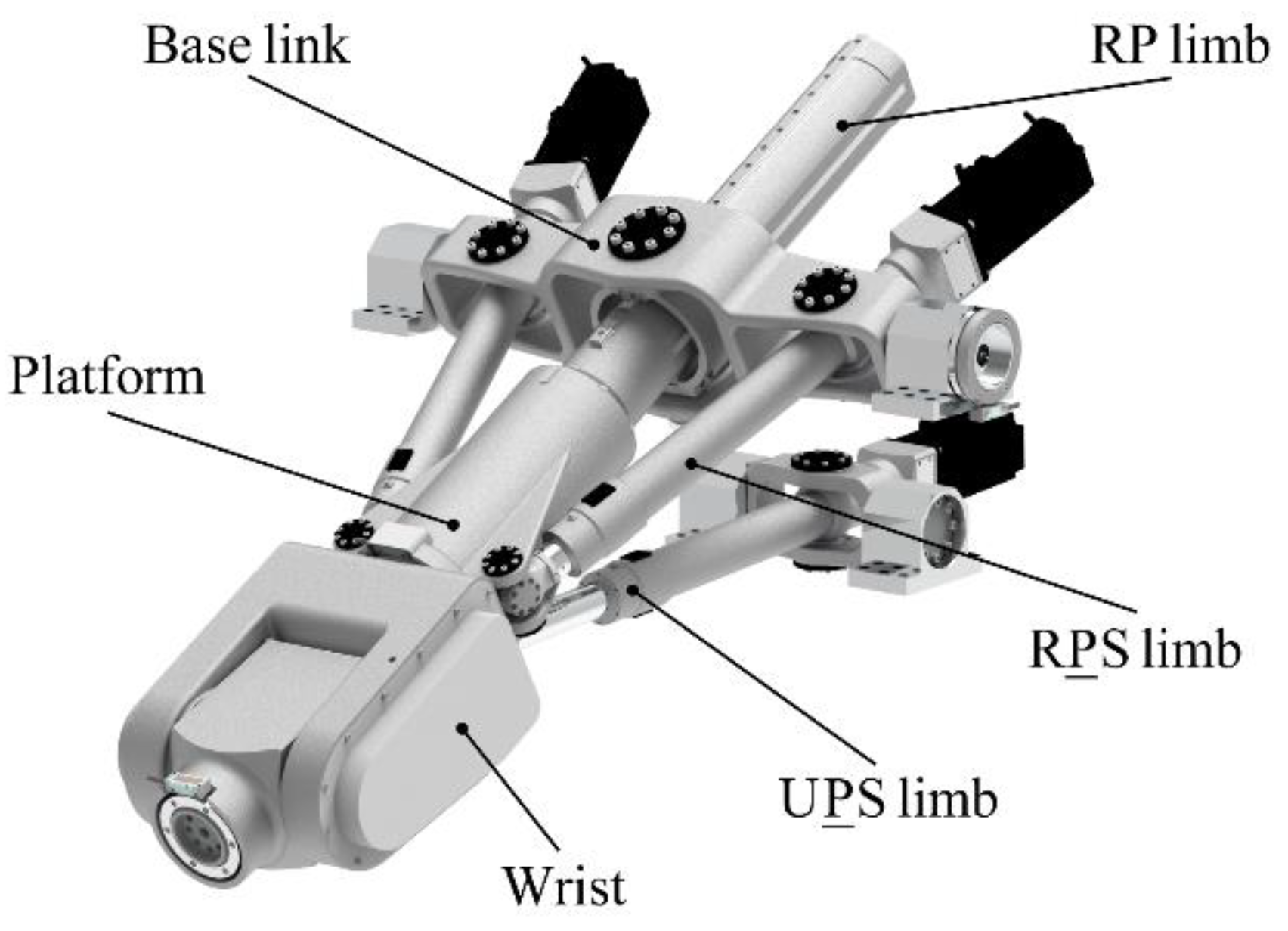
Figure 1 shows the 3D model of the TriMule robot. It mainly consists of a 3-DOF parallel mechanism and a 3-DOF wrist. The 1T2R parallel mechanism is composed of a 6-DOF U
PS limb and a 2-DOF planar parallel mechanism involving two actuated R
PS limbs and a passive RP limb. The planar parallel mechanism is connected to the base frame through a pair of R joints. The wrist is an
RRR series mechanism with three axes intersecting at a common point. Here, R, U, S, and P represent the revolute joint, universal joint, spherical joint, and prismatic joint, respectively. The underlined
R and
P represent the actuated revolute joint and prismatic joint, respectively.
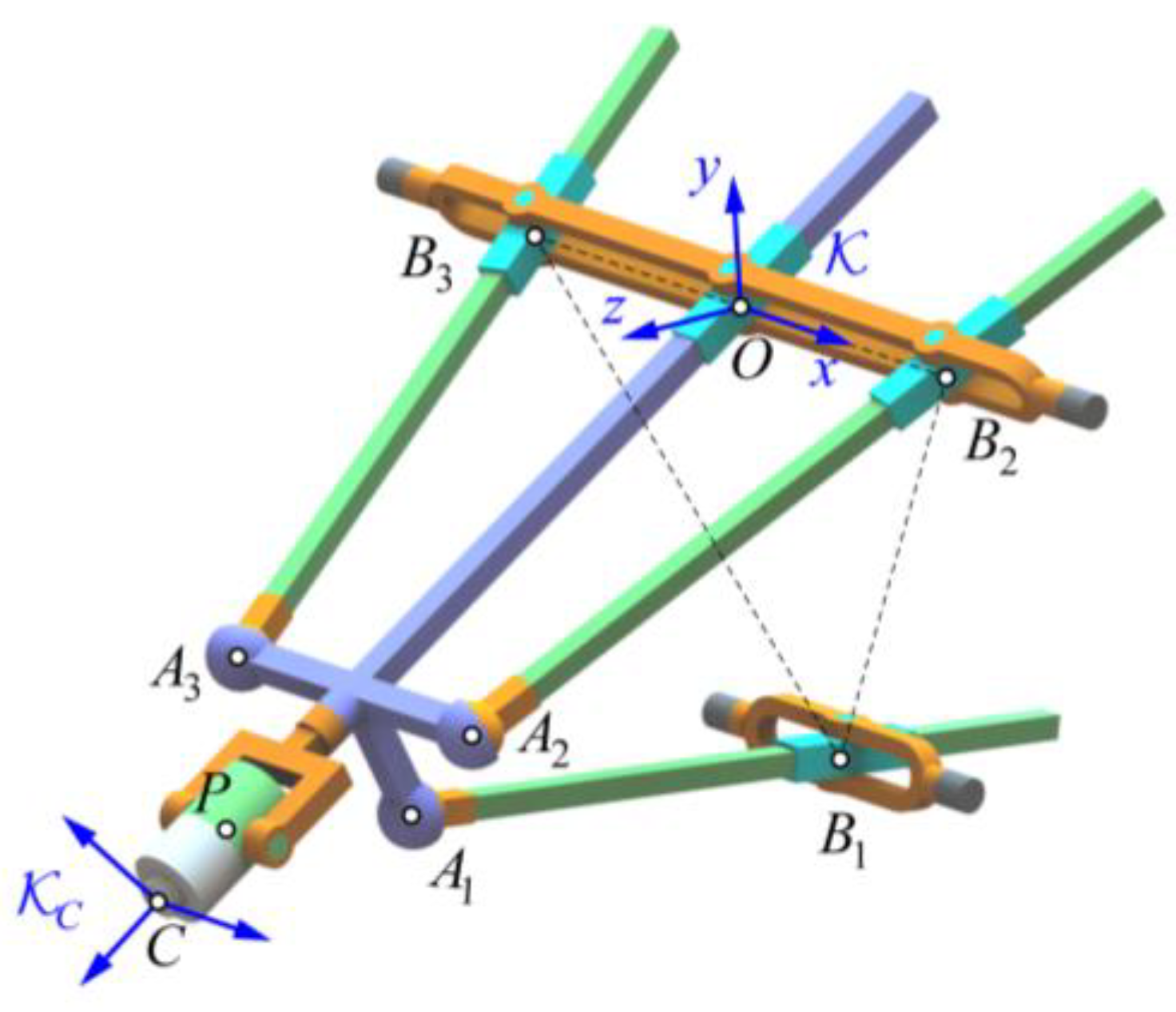
As illustrated in
Figure 2, we number the U
PS limb and two actuated R
PS limbs as limbs 1, 2, and 3, respectively. The passive RP limb together with the wrist is limb 4.
is the center of the U joint of limb 1;
is the intersections of the R joints of limb
i and the rotation axis of the planar parallel mechanism defined by the R joints connecting to the base frame; and
is the center of the S joint of limb
i. Let
P be the intersection of three orthogonal axes of the wrist and
C be the tool center point (TCP) of the robot end-effector. The base frame
is placed at point
O, the intersection of the R joint of the RP limb and the rotation axis of the planar parallel mechanism, with its
z-axis normal to
, the triangle with vertices at points
, and its
x-axis coincident with
3. Motion Decomposition and Measurement
This section focuses on the decomposition measurement for a 6-DOF hybrid robot. It involves the principle of motion decomposition and the implementation process of decomposition measurement.
3.1. Principle of Motion Decomposition
Sufficient pose measurement data are the basis of data-driven calibration and are crucial to a good compensation effect. However, the measurement data required by accurate calibration exponentially increase with increasing dimensions of the joint space. The curse of dimensionality is the main challenge in measurement tasks. Decomposition measurement is an effective approach to solve this problem. In previous research [
40], we decomposed a 5-DOF hybrid robot into a 2-DOF wrist and a 3-DOF parallel mechanism through mechanism decomposition. The pose errors of the two substructures are measured respectively and then composed to obtain those of the hybrid robot, effectively improving the measurement efficiency. However, the pose errors of the parallel mechanism can hardly be measured directly due to the occlusion of the wrist. An additional transfer frame must be established to connect the two substructures so that indirect measurement can be completed with the help of the end effector. As a result, it involves not only transformation errors but also a heavy burden in the measurement.
To solve these troubles, we proposed a motion decomposition method in this paper. The arbitrary motion of the robot is equivalently decomposed into three independent sub-motions. The sub-motions are achieved by driving the actuated joints according to specific rules. Consequently, decomposition measurement can be realized by only measuring the end pose of the robot, which is more practical and efficient.
According to the mechanism characteristics of TriMule, we partition the joint variables
into two subsets,
and
, where
u contains the joint variables of the parallel mechanism and
v contains the joint variables of the wrist. The mappings between the robot joint space and the operation space are defined as the kinematics functions
, and the corresponding motions can be expressed by the homogeneous transformation matrices
. Hence, the forward kinematic function of the hybrid robot
can be written as:
where
and
are the kinematic functions of the wrist and the parallel mechanism defined by
v and
u, respectively.
Then, Equation (1) can be equivalently transformed into:
where
is an arbitrarily fixed value for
u,
represents the motion of the parallel mechanism associated with
,
is an arbitrarily fixed value for
v, and
represents the motion of the wrist associated with
.
Finally, substituting Equation (1) into Equation (2) results in the motion decomposition formula:
where
,
, and
.
Hence, an arbitrary motion of the hybrid robot can be equivalently decomposed into three independent motions: , , and .
3.2. Decomposition Measurement and Composition
According to the definition of the kinematics functions
, Equation (3) can be rewritten as
where
,
,
, and
represent the poses of the hybrid robot at different configurations
,
,
, and
, respectively.
Thus, for a certain motion , except for the direct measurement at configuration , we can also measure the poses of the hybrid robot , , and at another three specific configurations, , , and , respectively, and then obtain the required pose through composition. It is worth noting that is an arbitrarily fixed value for , and , are related to and .
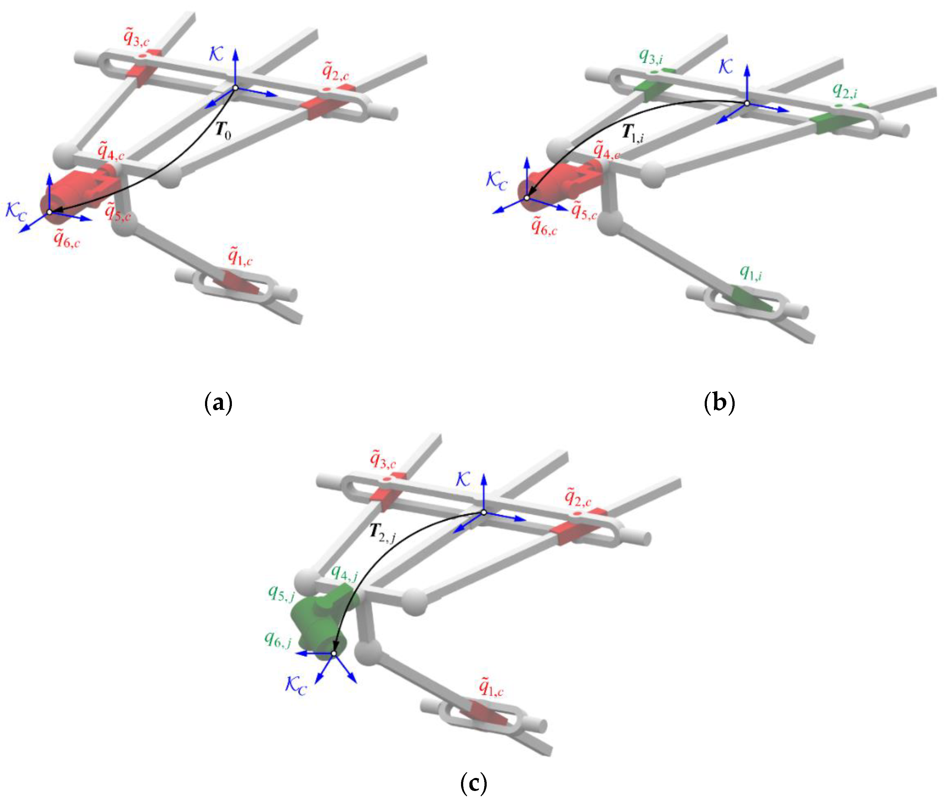
Although the decomposition measurement demonstrates no obvious advantages for a single configuration and even increases the measurement task, it has great advantages in terms of measurement efficiency for massive measurement tasks. In addition to
Figure 3, the detailed steps of the method are described as follows. For convenience of description, the stationary joints of the hybrid robot are marked in red, and the moving joints are marked in green.
(1) The base frame
is established as defined in
Section 2, and an end frame
is set up at the robot end-effector (see
Figure 3). All measurements hereinafter are conducted in the base frame
, and
denotes the transformation matrix of frame
with respect to frame
for different configurations
.
(2) An arbitrary fixed value
is set as the reference configuration. The hybrid robot is moved to
, and its end pose
is measured, as shown in
Figure 3a.
(3) The
m measurement configurations
are uniformly selected in the joint space of the parallel mechanism. The hybrid robot is moved to each configuration
successively by keeping the wrist stationary at the reference configuration and moving the parallel mechanism independently. Next, the end pose of the robot
is measured at each configuration, as shown in
Figure 3b.
(4) The
n measurement configurations
are uniformly selected in the joint space of the wrist. The hybrid robot is moved to each configuration
successively by keeping the parallel mechanism stationary at the reference configuration and moving the wrist independently. Next, the end pose of robot
is measured at each configuration, as shown in
Figure 3c.
The composition is conducted according to Equation (4) so that we can obtain the end poses of the hybrid robot
at a large number of combined configurations
:
The six-dimensional joint space of the hybrid robot is decomposed into two three-dimensional subspaces through decomposition measurement. Assuming that m and n measurement configurations are planned in two subspaces, the robot poses at configurations can be easily obtained by only measurements, which greatly improves the measurement efficiency. Moreover, the method is superior in terms of measurement efficiency with the increase of the measurement configurations m and n.
4. Improved Data-Driven Methodology for Calibration
In this section, an improved data-driven methodology is proposed. It directly establishes the mapping between the nominal joint variables and joint compensation values based on a BPNN and then conducts the training by a unique algorithm involving the robot inverse kinematics.
4.1. Principle of the Improved Data-Driven Methodology
The existing data-driven methods usually include two steps: estimation and compensation. First, an error estimation model is established based on the data-driven approach. Next, compensation is implemented based on the estimated values, as described in our previous research [
40]. Although the method realized real-time compensation and achieved a high calibration accuracy in the whole workspace of the robot, it inevitably introduces the estimated residual in theory. Moreover, the joint compensation values are calculated based on Jacobian iteration, which may cause a heavy computational burden in the sample set construction. Hence, an improved data-driven methodology is proposed. By merging the processes of estimation and compensation, a mapping between the nominal joint variables and joint compensation values is established based on a BPNN and then trained directly using the measurement data through a unique training algorithm involving the robot inverse kinematics.
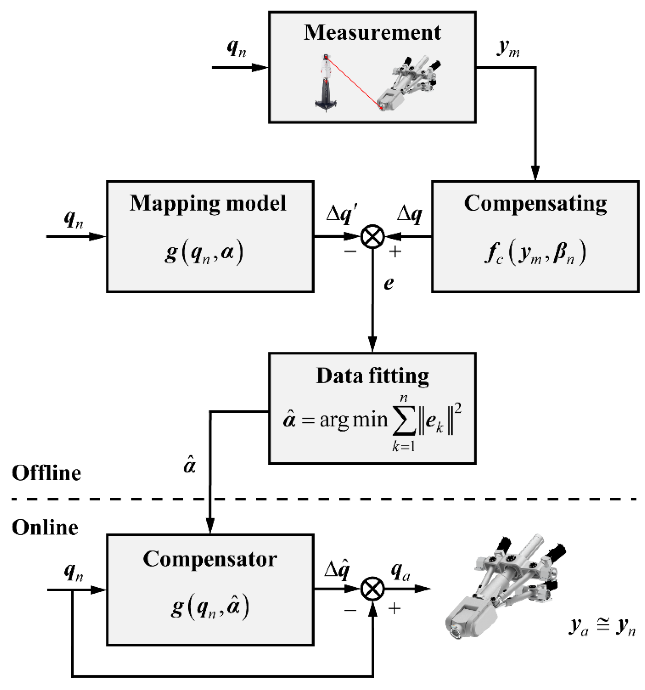
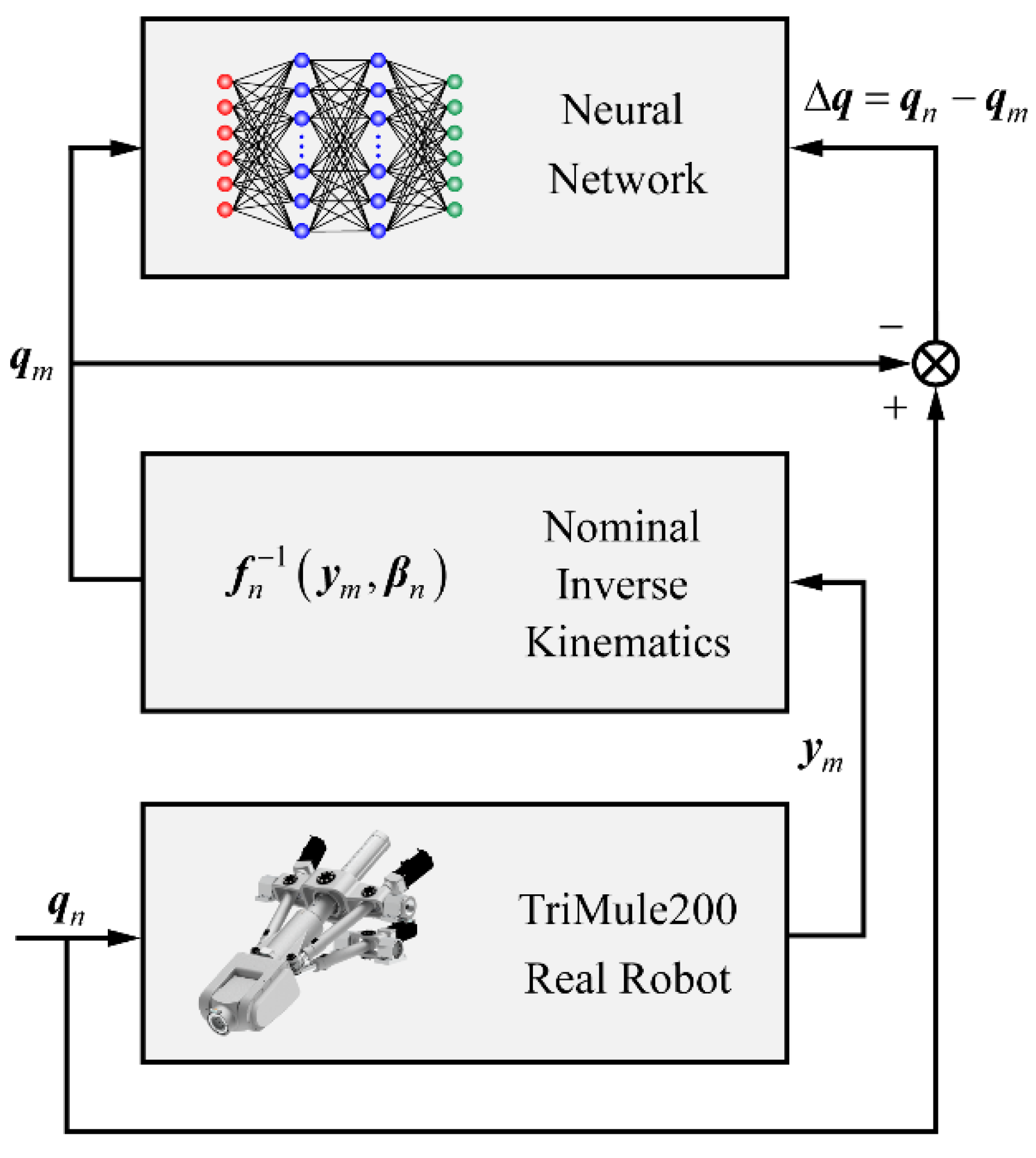
As shown in
Figure 4, the data-driven methodology mainly contains two steps: offline calibration and online compensation. First, measurement is conducted to obtain the actual pose
of the hybrid robot at the nominal joint variable
, and the joint compensation value
is computed according to the robot mechanism model such as the kinematic and Jacobian models. Second, the mapping
between the nominal joint variables and joint compensation values is established based on the data-driven methodology, where
can be a polynomial function, interpolation function, or neural network, and
represents the parameter to be determined by the mapping. Next, parameter
is fitted to minimize the predicted residuals for all measurement configurations. Finally, the compensator
is embedded into the robot control system for online compensation. For a certain joint command
, the joint compensation value
is obtained according to the compensator, and the corrected joint variable
is calculated by
so that the robot’s actual pose
can be as close as possible to the desired pose
.
The method establishes the mapping model between the nominal joint variables and joint compensation values, which can be directly used for online compensation after data fitting, voiding the troubles of error estimation and iterative calculation in compensation. To guarantee the implementation effect, the following two core problems need to be solved: (1) how to establish an accurate mapping model; and (2) how to obtain accurate joint compensation value.
4.2. Mapping Model Designing
The first step is to establish an appropriate mapping model. According to previous research, polynomial fitting can accurately estimate the position errors of robots on Cartesian space trajectory [
22]. However, for the compensation of pose errors in the whole workspace of a 6-DOF robot, constructing high-order polynomials with six variables will involve too many coefficient terms, which will cause much trouble in parameter identification [
23]. Furthermore, building up a query table of spatial interpolation in the whole workspace of the robot requires the expensive cost of time and storage space [
9], so it is tough to implement in practice. The neural network, which has a strong ability for nonlinear mapping and generalization, can fit any complex nonlinear mapping. In recent years, a back propagation neural network (BPNN) has been gradually applied in robot calibration by many scholars [
28,
29]. Along this track, a BPNN is built to describe the mapping between the nominal joint variables and joint compensation values in the whole workspace of the robot.
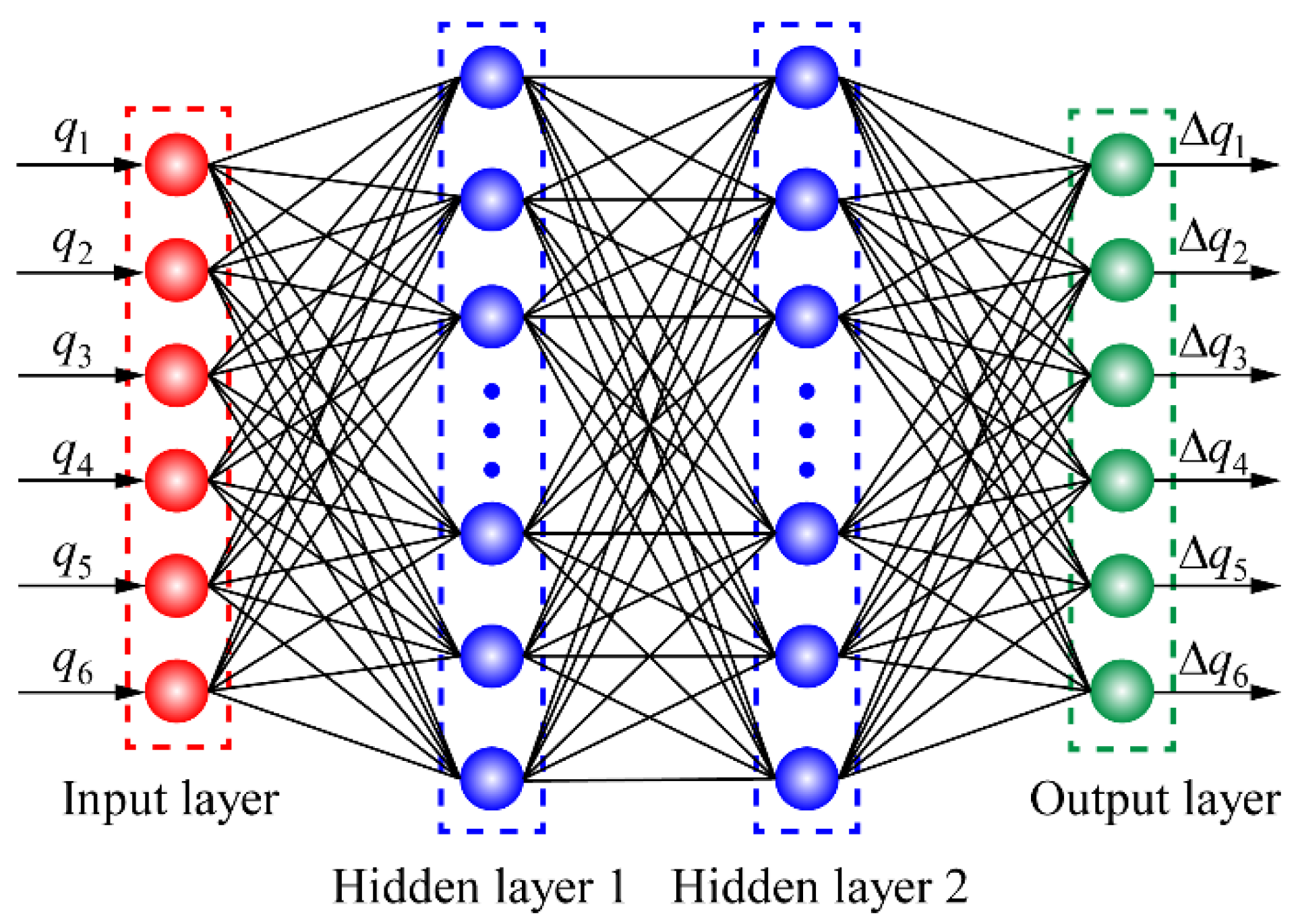
Taking the nominal joint variable and corresponding compensation value as the input and output, respectively, a BPNN is constructed, as illustrated in
Figure 5. Both the input and output layers consist of six neurons, representing six elements of the nominal joint variable
and the joint compensation value
, respectively. According to some successful experiences [
31], it has two hidden layers, and the tan-sigmoid function and linear function are taken as the activation functions of the hidden layer and the output layer, respectively.
4.3. Network Training
Next, a unique network-training algorithm is proposed based on the robot inverse kinematics, which can train the network directly using the pre-measured robot poses, avoiding the troubles of calculating the pose errors and solving the joint compensation values. The principle of network training is shown in
Figure 6.
When the nominal joint variable is input, the robot moves to rather than the desired pose . Next, the nominal joint variable of pose is computed through the nominal inverse kinematics. Assuming that the desired pose of the robot is , the joint command theoretically needs to be input to the robot. However, the robot cannot move to due to various errors in the robot system. The robot will move to exactly when the joint command is input at the beginning. Hence, the joint variable can be regarded as the corrected joint variable of the desired pose , and is the corresponding joint compensation value of robot configuration . It is worth noting that here is the joint compensation value corresponding to joint variable rather than . Therefore, the neural network should be trained with and as the input and output, respectively.
Following the principle above, Algorithm 1 is proposed for training the BPNN:
| Algorithm 1: Training of BPNN |
1 foreach do;
2 ;
3 ;
4 ;
5 as output. |
Through the algorithm, the BPNN can be trained directly based on the pre-measured robot poses and the nominal inverse kinematics, which avoids the process of solving robot pose errors and the complex iterative calculation in error compensation. In terms of compensation accuracy, the real compensation value of the robot can be obtained on the premise of ignoring the measurement errors rather than the approximate value obtained by iterative calculation.
5. Experiments
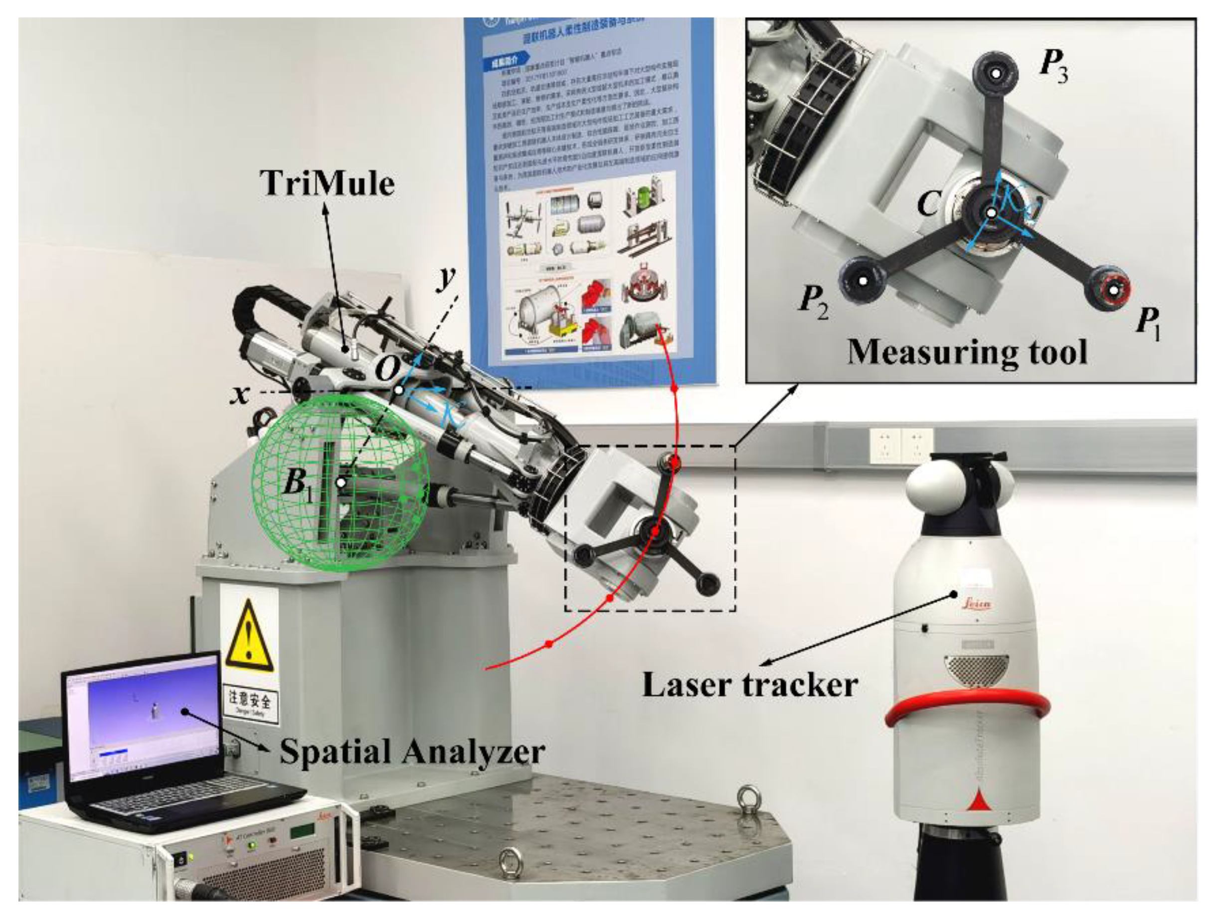
To demonstrate the effectiveness of the methodology, the validation experiments are carried out as shown in
Figure 7. A TriMule 200 robot, which has a repeatability accuracy of 0.0197 mm/0.0041 deg, is taken as the verification platform. The measuring instrument is a Leica AT901-LR laser tracker that has a maximal observed deviation of 0.005 mm/m. In addition, all measurements are conducted under static and no-load conditions.
Before pose measurement, the base frame
is registered in the measuring software (Spatial Analyzer) according to its definition, as illustrated in
Section 2. The
x-axis is constructed by fitting the arc trajectory marked in red, which is formed by the spherically mounted retroreflector (SMR) attached to the end of the robot. The center
of the U joint is constructed by fitting the green spherical surface, which is formed by another SMR fixed at limb 1. A normal line from
to the
x-axis is constructed as the
y-axis, and intersection
O is defined as the origin. Next, a base frame
is constructed according to the right hand rule (see
Figure 7). A specialized measuring tool is connected to the end effector with its centers of the three SMRs defined as
,
, and
. The end frame
is placed at point
C, which is the center of
,
, and
. Thus, the end pose
can be obtained by measuring
,
, and
as follows:
with
where
is aligned with
, and
is normal to
.
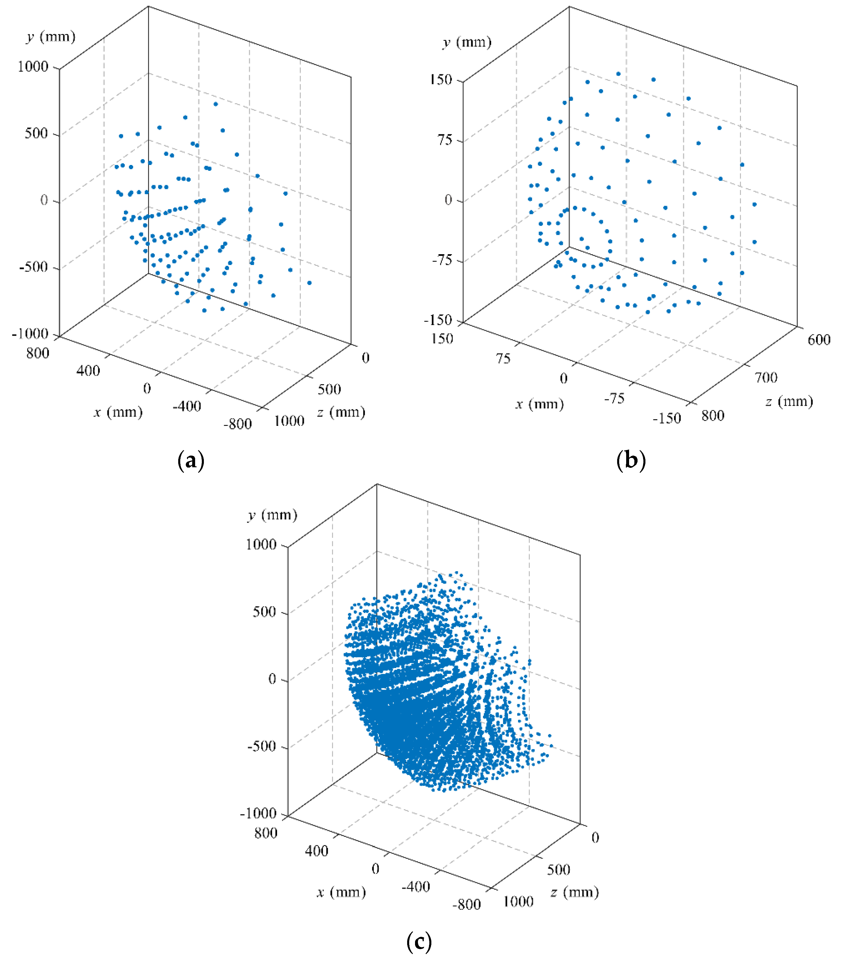
The decomposition measurement methodology is adopted to efficiently acquire the robot poses in the whole workspace. The joint space of the hybrid robot is divided into two subspaces, i.e., the joint space of the parallel mechanism (W1) composed of joints 1, 2, and 3 and the joint space of the wrist (W2) consisting of joints 4, 5, and 6. The joint space of the hybrid robot is defined by the motion ranges of the six actuated joints, as shown in
Table 1. To sample the robot poses over the entire workspace, W1 and W2 are discretized into two sets of three-dimensional grid elements, of which vertices are taken as the sampling configurations of W1 and W2, respectively. The discretization rules are as follows: (1) Joints 1, 2, and 3 are divided by a sampling interval of 60 mm so that W1 is discretized into a group of 125 sampling configurations. (2) The sampling intervals of 60°, 22.5°, and 45° are adopted for joints 4, 5, and 6, respectively, to discretize W2 into a group of 175 sampling configurations.
The home pose of the robot is taken as the reference configuration for convenience. Following the detailed processes described in
Section 3.2, the end poses of the robot are measured at the sampling configurations of W1 and W2, as illustrated in
Figure 8a,b.
Figure 8c shows the distribution diagram of the tool center point (TCP) in the robot workspace, which is obtained by composing the sampling configurations of W1 and W2. Consequently, a group of 21,875 samples are acquired with only 300 measurements.
To prove the effectiveness of the proposed method, it is compared with the calibration method in reference [
38]. For more detailed steps of the comparative experiment, please refer to [
38], which will not be repeated here. This paper only gives the necessary measurement process, network training parameters, and error compensation results.
Both methods adopt the same sampling configurations as described before. The detailed measurement procedures and sampling time are shown in
Table 2 and
Table 3, respectively. The experimental results show that both methods effectively improve the measurement efficiency, which can obtain massive sampling data in the whole workspace of the robot within 160 min. Although the proposed method does not show significant advantages in sampling time, it avoids the establishment of the transfer frame and frequent coordinate system transformation in the measurement. All data are directly measured based on the robot base frame and the end measuring tool. Thus, it is more practical and efficient for on-site implementation.
Next, two BPNNs are trained by two methods, respectively, to compensate for the robot pose errors. Since the hyperparameters of the network will directly affect its training performance, a series of comparative experiments are conducted to determine the optimal number of hidden layer neurons. The number of neurons is increased gradually to search and verify the optimal architecture, which is judged by the root mean square error (RMSE) of the testing and training sets [
21,
31].
Table 4 shows the specific training parameters of two neural networks. It is worth noting that the networks are trained by two different sample sets constructed by the proposed and comparative methods, respectively, although they have the same number of samples. Finally, the BPNNs are embedded into the robot to realize online compensation.
The uniform sampling intervals of 80 mm, 80 mm, 80 mm, 90°, 30°, and 60° are adopted for joints 1, 2, 3, 4, 5, and 6 to discretize the whole workspace of the hybrid robot into 5120 poses, from which 100 poses are randomly selected as validation configurations, as shown in
Figure 9. It is worth mentioning that none of the discretization poses overlap the sampling poses. The actual pose of the robot is measured before and after compensation and then compared with its nominal pose. The volumetric orientation error
and volumetric position error
(simplified as the orientation and position errors) are taken as the evaluation index of robot accuracy.
Figure 10 and
Figure 11 and
Table 5 show the experimental results. After compensation by the proposed method, the robot’s maximum position/orientation errors are reduced to 0.085 mm/0.022 deg, which is 91.16%/88.17% lower than 0.962 mm/0.186 deg before compensation, respectively, and the mean position/orientation errors are reduced by 91.22%/89.74% to 0.049 mm/0.012 deg, respectively. After compensation by the comparative method, the maximum position/orientation errors have decreased to 0.098 mm/0.024 deg, which is 89.81%/86.56% lower than before compensation, and the mean position/orientation errors are reduced by 89.96%/88.73% to 0.056 mm/0.014 deg, respectively. Thus, we can conclude that the methodology can effectively improve the pose accuracy in the whole workspace of the robot.
6. Conclusions
This paper proposes an improved data-driven calibration method for a 6-DOF hybrid robot. It mainly focuses on enhancing calibration efficiency and practicability. The following conclusions are drawn.
(1) A decomposition measurement method is proposed to overcome the curse of dimensionality in the measurement of data-driven calibration. An arbitrary motion of the hybrid robot is equivalently decomposed into three independent sub-motions through motion decomposition. The sub-motions are sequentially combined according to specific motion rules. Thus, a large number of robot poses can be acquired over the entire workspace with a limited number of measurements.
(2) An improved data-driven methodology is proposed to replace the traditional processes of error estimation and compensation to improve the practicability in field applications. The mapping between the nominal joint variables and joint compensation values is established based on a BPNN. Next, it is trained directly using the measurement data of robot poses through a unique training algorithm involving the robot inverse kinematics.
(3) The experimental results demonstrate the effectiveness of the method. The robot’s maximal position/orientation errors are reduced by 91.16%/88.17% to 0.085 mm/0.022 deg after calibration.
(4) The proposed method can also be applied to other serial or hybrid robots as a general methodology.
In the future, we will continue to refine this method. In measurement, the relationship between the distributions of sampling configurations and calibration accuracy has to be further investigated to provide guidance for sampling configuration optimization. In network training, the research on an intelligent optimization algorithm of network structure will be carried out to replace the complex comparative experiments at present.


