Experimental Study of Robotic Polishing Process for Complex Violin Surface

Abstract

This paper presents a robotic polishing process for complex violin surfaces to increase efficiency and minimize the cost and consumed time caused by using labor and traditional polishing machines. The polishing process is implemented based on modeling a smooth path, controlled contact force embedded with gravity compensation and material removal depth. A cubic Non-Uniform Rational Bases-Spline (NURBS) interpolation curve combined with an S-curve trajectory model is used to generate a smooth polishing path on a complex violin surface to achieve stable motion during the polishing process. An online admittance controller added to the fast gravity compensation algorithm maintains an accurate polishing force for equal removal depth on all polished surface areas. Then, based on Pythagorean theory, the removal depth model is calculated for the violin’s complex surface before and after polishing to estimate the accuracy of the polishing process. Experimental studies were conducted by polishing a wooden surface using the 6DOF robot manipulator to validate this methodology. The experimental results demonstrated that the robot had accurate polishing force based on the online admittance controller with gravity compensation. It also showed a precise proportional uniformity of removal depths at the different normal forces of 10, 15, and 20 N. The final results indicated that the proposed experimental polishing approach is accurate and polishes complex surfaces effectively.

1. Introduction

The polishing process is commonly used in the manufacturing field to handle simple surface damage, reduce roughness [1,2], and achieve shine [3,4,5]. Polishing is essential in many industries requiring accuracy for surfaces, such as manufacturing molds, aircraft airfoils, ship propellers, and many other complex surfaces [6,7]. At present, the polishing of these surfaces is performed manually, which is time-consuming and costly, requiring experienced laborers; plus, a steady polishing process is difficult to maintain manually [8,9,10]. In addition, manual polishing can cause many diseases related to the respiratory and musculoskeletal systems [11], negatively affecting worker health. Therefore, an automatic polishing system is required to eliminate these issues and produce desired properties, such as improved quality, higher production yield [12,13], reduced time consumption [14,15], higher accuracy, and better reliability [16,17,18,19]. An alternative solution to manual polishing is an industrial robot [20]. Generally, robotic polishing processes have attracted researchers and companies in recent years [21]. In addition, a robotic polishing system can finish different workpiece shapes, such as simple, curved, or complex surfaces. This ability makes the industrial robot an effective and economical solution for polishing, especially for surfaces with complex geometries [22]. The robotic polishing system combines various related robotic sciences to automate the process and achieve high-quality polishing. These sciences include robot motion planning as a polishing path, force control, and material removal depth modeling. The key solution to achieving high-quality polishing is maintaining a consistent material removal depth over the entire polished surface. To achieve this solution, a smooth polishing path should be designed in addition to applying accurately controlled constant contact force to improve surface roughness [23,24,25,26], which is challenging on complex surfaces [27,28,29].

Many studies have been carried out on the robotic polishing of complex surfaces to minimize cost and enhance the process quality. For instance, Xu et al. [30] proposed a hybrid force/position controller approach. With the complexity between the robot and the unknown environment, they added a proportional-integral/proportional-derivative (PI/PD) controller to maintain constant contact force because the hybrid force/position control method could not be directly applied to the machining of complex parts. In addition, the study of [9] offered the methodology adopted for a robotic polishing system for polishing curved surfaces to minimize cost and improve quality compared to manual finishing operations. They proposed an algorithm for planning the polishing tool location and posture with force control. The results showed that the proposed automatic polishing system could polish a curved surface and achieve a mirror effect on the surface of the mold part. Similarly, Mohsin et al. [31] studied an effective method for the robotic polishing of a complex curved surface based on tool path planning with controlled force and polishing parameters. The proposed method was applied for the polishing of an eyeglass frame. In a similar direction, the grinding process uses the same methodologies as the polishing process; however, they exhibit slight differences. For example, grinding removes saw marks and levels and cleans the specimen surface, while polishing removes the artifacts of grinding but very little stock. In addition, grinding uses fixed abrasive particles bonded to the paper or platen for fast stock removal. Polishing uses free abrasives on a cloth; the abrasive particles are suspended in a lubricant and can roll or slide across the cloth and specimen. In this direction, Zhu et al. [24,32] presented a robotic belt grinding system and studied the effects of force components on surface roughness under various contact force situations. The final results showed that the constant force integrated with the optimal modeled parameters was effective at accurately grinding the turbine blades as complex surfaces.

In other research, Yu et al. [33] developed a new active end-effector for a robotic polishing system on complex parts; a hybrid force controller based on a fuzzy proportional-integral-derivative (PID) controller and gravity compensation achieved the contact force between the polishing tool and the part. The verification experiments were conducted using the proposed robotic polishing system on a complex polymethyl methacrylate (PMMA) part. In the same direction, Tian et al. [34] presented a methodology for a robotic polishing end-effector using position/posture and force-decoupling control. In addition, Ding et al. [35] proposed a method for polishing complex concave cavity surfaces with an industrial robot based on an adaptive PI force control algorithm and planning trajectory with the normal vector. The simulation and experimental results showed that this method could achieve the polishing of the concave cavity surface. Fengyun and Sheng [36] introduced a robotic polishing system instead of manual polishing based on trajectory generating. The robot polishing path was generated from the cutter location information taken from the postprocessor of a CAD system. Hahnel et al. [37] performed an experimental study on a complex surface sample to show the automated finishing process for molds and dyes. The test was conducted by defining the tool path approach for automatic processes with guidable process parameters, including contact force, feed rate, and spindle speed. In another study, Huang et al. [38] proposed a polishing system based on force control and performs offline programming of path planning of blade polishing by the robot through analysis of the damage of the contact area between the blade surface and polishing wheel using the Douglas–Peucker algorithm. Mohsin et al. [39] also discussed the robotic polishing process by organizing and improving the path planning for free-form surfaces under controlled force. They compared the optimized path planning concept for the symmetrical free-form surfaces to other techniques in terms of quality and accuracy. Ochoa and Cortesao [40] presented a computed torque impedance position and force control method for robotic assistance mold polishing based on human skills. The approach was validated through co-manipulation and free-hand modes.

The above-mentioned studies focused on the robotic polishing process on complex surfaces based on tool path planning under a force control algorithm to achieve a high accuracy and quality of polished surfaces. An equal material removal rate is considered a key solution for good polishing results, mainly depending on a smooth polishing path and an accurate force controller. Regarding a complex surface, maintaining constant contact polishing force and a smooth path cannot be obtained accurately using traditional force algorithms and existing motion planning control methods. Motivated by these issues, we propose a robotic polishing process for a complex surface (i.e., violin) composed of wood encountered by the Finelegend factory in Taizhou, China.

This study introduces an efficient robotic polishing process to achieve good polishing results on a violin’s complex surface. The contributions of this approach are a smooth polishing path methodology through combining the NURBS interpolation curve with an S-curve trajectory, incorporating a novel accurate admittance force controller combined with a gravity compensation algorithm, and then calculating the removal depth on a violin surface before and after the polishing process simply through the Pythagorean theorem. Finally, we conducted experiments and reported the results achieved by the precision polishing of the violin’s complex surface.

The rest of this paper is organized as follows: The smooth path polishing approach is described in Section 2. Next, Section 3 provides descriptions of the force control strategy and gravity compensation. The material removal profile measurement is presented in Section 4. Then, Section 5 reports the experimental results, and finally, the conclusions are drawn in Section 6.

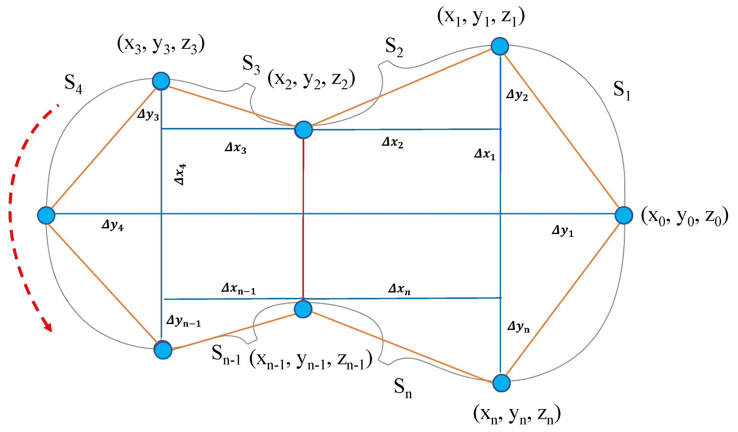
2. Smooth Polishing Path

This section introduces the mathematical model of the path used to polish complex violin surfaces. First, a combination of NURBS with the S-curve model is utilized to achieve a smooth and continuous polishing path. Then, the spherical quadrangle interpolation (squad) quaternion attitude interpolation between two adjacent quaternions is used to obtain discrete points corresponding to the NURBS curve.

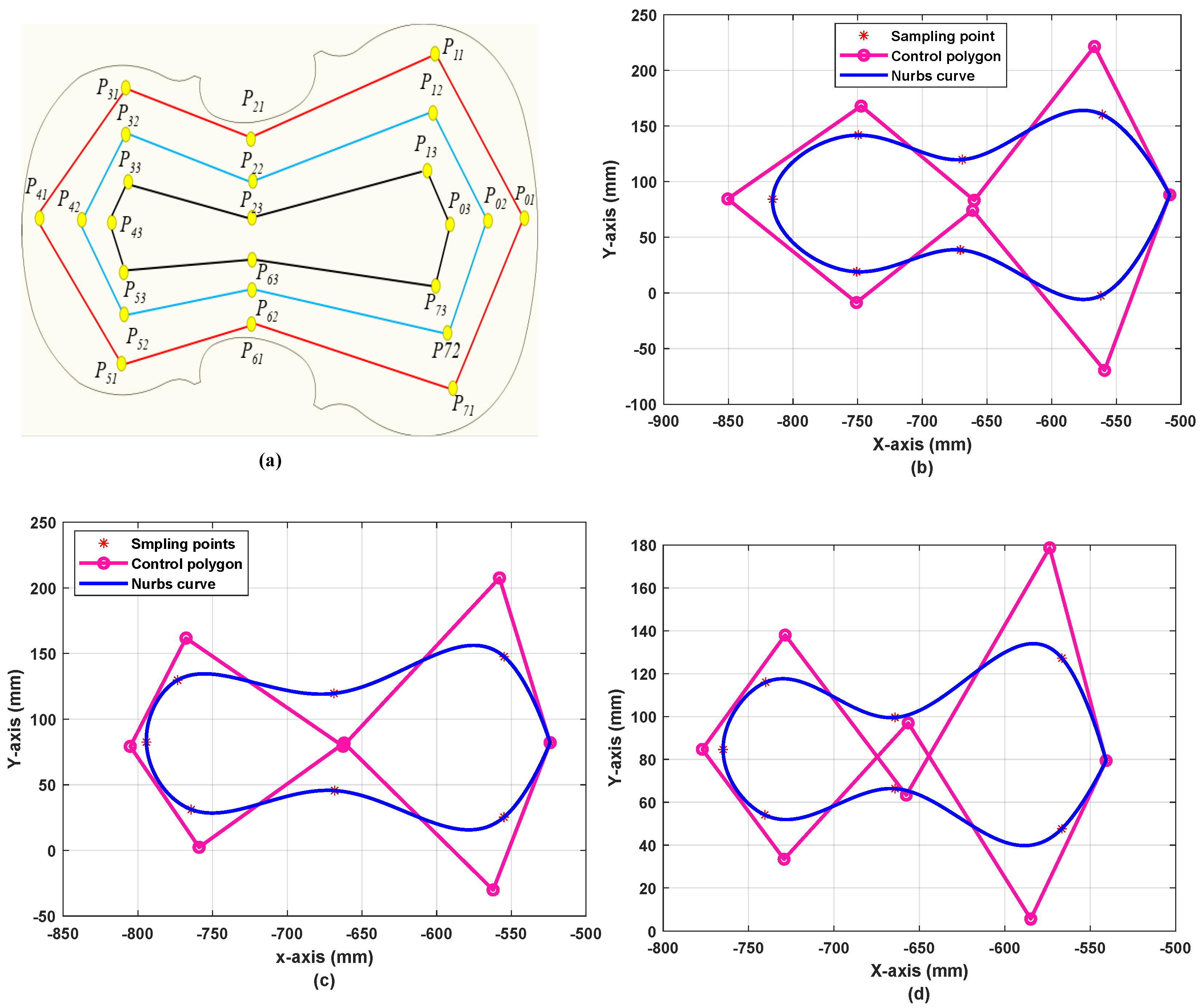
2.1. Nurbs Interpolation Curve

The NURBS comprises control points $P_i$ with number $\left(n\right)$, knot vector $u_i$, weights $w_i$, and the B-spline basis function $N_{i,p}\left(u\right)$ and its order p; the general form of the NURBS can be described as

$$C\left(u\right)=\frac{{\displaystyle \sum _{i=0}^n}{N}_{i,p}\left(u\right)w_i{P}_i}{{\displaystyle \sum _{i=0}^n}{N}_{i,p}\left(u\right)w_i}{u}_p\le u\le u_{n+1}$$

(1)

where the $N_{i,p}\left(u\right)$ cox-de Boor recursion formula for basis functions can be written as

$$\left\{\begin{array}{c}{N}_{i,0}\left(u\right)=\left\{\begin{array}{c}1when{u}_i\le u\le u_{i-1}\hfill \\ 0otherwise\hfill \end{array}\right.\hfill \\ N_{i,p}\left(u\right)=\frac{u-u_i}{u_{i+p}-u_i}{N}_{i,p-1}\left(u\right)+\frac{u_{i+p+1}-u}{u_{i+p-1}-u_{i+1}}{B}_{i+1,p-1}\left(u\right)\hfill \end{array}\right.$$

(2)

In the NURBS, knot-open uniform vectors interpolate the first and last control points, ensuring that the robot end-effector can pass through source and destination points. The multiplicity of the knot vector of the first and last pointx of an open uniform can be formulated as

$$u_i=\left\{\begin{array}{c}00\le i\le k\hfill \\ i-kk+1\le i\le n+1\hfill \end{array}\right.$$

(3)

The knot vector here is assumed at $k=3$ (cubic NURBS) as the following: $u_0=u_1$$=u_2=u_3=0$ and $u_i=i-k,ati=4,5,\dots ,n$. Assume that the sampled tool center points (TCP) are ${\left\{C_i\right\}}_{i=0}^n$ by taking the first and end points $c_0$ and $c_n$ as the source and destination control points of the NURBS interpolation curve, respectively. Then, considering the midpoints $c_2$, $c_3$, …, $c_{n-2}$ as the segments of the cubic NURBS interpolation curve, $c_1$ and $c_{n-1}$ are the points on the first and last segments, respectively; then, the control points are calculated as $n+1$. To determine the arc length of curve $c\left(u\right)$ of two parameters between [a, b], Simpson’s approximation approach is used [41], which can be expressed as

$$s=\underset{a}{\overset{b}{\int }}f\left(x\right)dx$$

(4)

The Simpson approximation formula in more detail can be described as

$$s=\underset{x_0}{\overset{x_4}{\int }}\frac{h}{12}(f_0+4f_1+2f_2+4f_3+f_4)$$

(5)

where $x_0=a,x_4=b,h=b-a,x_2=x_1+h,x_3=x_2+h;f_i=f\left(x_i\right),i=0,1,\dots 4$.

2.1.1. S-Curve Velocity Planning

To establish the continuity and easy interpolation of junctions between successive NURBS curves, the S-velocity shape is used. Parameters $q_0$, $q_1$, $v_0$, and $v_1$ are the position and velocity of the starting and end points, respectively, while $v_{max}$ and $a_{max}$ are the maximum speed and acceleration, respectively. At the uniform of acceleration segment of ${\mathrm{t}}_0\le \mathrm{t}\le {\mathrm{T}}_a$, take a constant value of $a_{max}$, so that the speed increases from ${\mathrm{v}}_0$ to ${\mathrm{v}}_{max}$. In the period ${\mathrm{T}}_a\le \mathrm{t}\le {\mathrm{T}}_a+{\mathrm{T}}_v$, the speed is constant at $v_{max}$. In addition, at a uniform of deceleration, where $T_a+T_v\le \mathrm{t}\le T_a+T_v+T_d$, slow down acceleration occurs at $-a_{max}$ to reduce the speed from $v_{max}$ to $v_1$.

2.1.2. S-Shape Speed Curve Algorithm Steps

• First, the total displacement between any two points according to [42] should be calculated by

  $$h{a}_{max}\ge v_{max}^2-\frac{v_0^2+v_1^2}{2}$$

  (6)

  where h is the total displacement, which is equal to $(q_1-q_0)$. From Equation (6), the peak velocity can be described as

  $$v_{lim}=\sqrt{h{a}_{max}+\frac{v_0^2+v_1^2}{2}}\le v_{max}$$

  (7)
  In this casewhen $v_{max}$ is actually reached and maintained during the constant velocity phase, $v_{\mathrm{v}}=v_{max}$; otherwise, $v_{\mathrm{v}}=v_{lim}$, where $v_{\mathrm{v}}$ according to [42] can be described as

  $$v_{\mathrm{v}}=\frac{1}{2}(v_0+v_1+a_{max}T-\sqrt{a_{max}^2{T}^2-4a_{max}h+2a_{max}(v_0+v_1)T-{(v_0+v_1)}^2}$$

  (8)
• Next, we calculate the length of the acceleration/deceleration periods and total time; so, in the case of $v_{\mathrm{v}}=v_{max}$; then,

  $$\left\{\begin{array}{c}{T}_a=\frac{\left(v_{max}-v_0\right)}{a_{max}}\hfill \\ T_d=\frac{\left(v_{max}-v_1\right)}{a_{max}}\hfill \\ T=\frac{h}{v_{max}}+\frac{v_{max}}{2a_{max}}(1-\frac{v_0}{v_{max}})+\frac{v_{max}}{2a_{max}}(1-\frac{v_1}{v_{max}})\hfill \end{array}\right.$$

  (9)
• Then, we determine the formula of each stage of the S-shaped speed curve as

$t\in (0,T_a)$:

$$\left\{\begin{array}{c}q=q_0+v_{0}t+\frac{a_{max}}{2}{t}^2\hfill \\ \frac{dq}{dt}=v_0+a_{max}t\hfill \\ \frac{d^{2}q}{d{t}^2}=a_{max}\hfill \end{array}\right.$$

(10)

$t\in (T_a,T_a+T_v)$:

$$\left\{\begin{array}{c}q=q_0+v_0\frac{T_a}{2}+v_{\mathrm{v}}(t-\frac{T_a}{2})\hfill \\ \frac{dq}{dt}=v_{\mathrm{v}}\hfill \\ \frac{d^{2}q}{d{t}^2}=0\hfill \end{array}\right.$$

(11)

$t\in (T_a+T_v,T_a+T_v+T_d$):

$$\left\{\begin{array}{c}q=q_1+v_1(t_1-t)+\frac{v_{\mathrm{v}}-v_1}{2T_d}{(t_1-t)}^2\hfill \\ \frac{dq}{dt}=v_1+\frac{v_{\mathrm{v}}-v_1}{2T_d}(t_1-t)\hfill \\ \frac{d^{2}q}{d{t}^2}=-\frac{v_{\mathrm{v}}-v_1}{2T_d}=-a_{max}\hfill \end{array}\right.$$

(12)

2.2. Quaternion Pose Squad Interpolation Method

The squad is a spline-based interpolation of rotation vectors: if the $q_n$ is a sequence of N quaternions, where $n=0$ to $N-1$, then smooth interpolation is given by the following equation

$$Squad(q_n,a_n,a_{n+1},q_{n+1};t)=Slerp(Slerp(q_n,q_{n+1};t),Slerp(Slerp(q_i,q_{i+1};t);2t(1-t))$$

(13)

where Slerp is shorthand for spherical linear interpolation, and

$$a_n=q_{n}exp(-\frac{log(q_n\ast q_{n-1})+log(q_n\ast q_{n+1}}{4})$$

(14)

where $q_n$ and $q_{n+1}$ are the start and end points of rotation, t is the interpolation parameter that lies in the interval [0, 1], and $a_n$ and $a_{n+1}$ are intermediate quaternions. Then, the use of squad can keep these two sections and transition smoothly.

3. Admittance Force Control Method with Gravity Compensation

Adjusting the contact force between the polishing tool and the workpiece is critical, where an accurate contact force results in the high quality of the polishing process. A proper force control method should be used to yield precise polishing results because the motion control system alone cannot polish surfaces accurately. The admittance controller is used in many applications that require a controlled interaction force [43] to regulate the applied force during polishing. The robot’s manipulator suffers from inaccurate contact force during an interaction, leading to poor polishing quality; thus, the controlled force method fixes this problem.

3.1. Controlled Contact Force

In this paper, the online admittance controller provides an accurately controlled contact force to the polishing process. To this end, an online environment stiffness uses the reference position and desired force and merges the contact force error with the damping force as a compensation procedure. For accurate interaction control, admittance parameters, mass-damper-spring ($M_r$, $B_r$, $K_r$), and desired position $X_d$ must be precisely calculated; the contact and desired forces according to the Figure 1 and Figure 2 can be written as

$$\left\{\begin{array}{c}{F}_e=K_e(X_e-X_a)\hfill \\ F_d=M_r\delta \ddot{X}+B_r\delta \dot{X}+K_r\delta X\hfill \end{array}\right.$$

(15)

where $K_e$ is the environment stiffness, $K_r$ is robot stiffness, $X_e$ is environment location, and $X_a$ is the actual position of the end-effector. Assume that the robot is ideal; then, $X_a$ should equal $X_t$, where $X_t$ is transmitted position. With $X_a$ = $X_t$, we obtain

$$K_e(X_e-X_t)-F_d=M_r\delta \ddot{X}+B_r\delta \dot{X}+K_r\delta X$$

(16)

where $\delta X=X_t-X_d$. By considering the steady-state position error for both sides, Equation (16) can be simplified as

$$K_e(X_e-X_d)-K_e(X_t-X_d)=K_r(X_t-X_d)$$

(17)

The steady-state position error is exactly $\left(\delta X\right)$, as

$$K_r{e}_{ss}^p=K_e(X_e-X_d)-K_e{e}_{ss}^p$$

(18)

By rearrangement of Equation (18) yields

$$e_{ss}^p=\frac{K_e(X_e-X_d)}{K_r+K_e}$$

(19)

Based on $e_{ss}^p$ and desired force $F_d$, the desired $K_r$ can be calculated as

$$\begin{array}{c}{K}_r=\left(F_d\right)/(X_t-X_d)=\hfill \\ \left(F_d\right)/e_{ss}^p=\frac{F_d(K_r+K_e)}{K_e(X_e-X_d)}\hfill \end{array}$$

(20)

Reversing Equation (20), we can obtain the estimated environment stiffness by

$${\stackrel{⌢}{K}}_e=\frac{F_d{K}_r}{K_r(X_e-X_d)-F_d}$$

(21)

Actually, to achieve an accurate contact force $K_e\gg K_r$ according to the steady-state force error, the stiffness ratio is $\frac{K_e}{K_r}\gg 1$ to obtain an online environment stiffness from Equation (21) in accordance with the condition of contact force accuracy. Then, to make environment stiffness adjustable according to the robot stiffness, we can express it as

$$K_e^{*}=\left(\frac{K_e}{K_r}\right){\stackrel{⌢}{K}}_e=\left(\frac{K_e}{K_r}\right)\left(\frac{F_d{K}_r}{K_r(X_e-X_d)-F_d}\right)$$

(22)

where $K_e^{*}$ is online stiffness and $K_e$ is the constant environment stiffness, which is always considered as a large rigid value compared to robot stiffness. This method calculates an online environment stiffness using the above constant environment stiffness and some selected robot stiffness values to achieve accurate position tracking.

The proposed damping force law used to adapt an online environment stiffness to help eliminate force error as a second step of this controller as

$$\delta {\mathrm{F}}^{\prime }=F_d-F_e^{*}+B_r{\dot{X}}_d$$

(23)

Equation (23) can be rewritten by the following expression:

$$\delta F^{\prime }=F_d-K_e^{*}(X_e-X_t)+B_r{\dot{X}}_d$$

(24)

For a practical interaction control of the robot and its environment, the modified admittance controller in discrete form can be determined as

$$\left\{\begin{array}{c}{\ddot{X}}_t\left(t\right)={\ddot{X}}_d\left(t\right)+1/\phantom{1M_r}{M}_r(\delta {\mathrm{F}}^{\prime }\left(\mathrm{t}\right)-\hfill \\ B_r({\dot{X}}_t(t-1)-2{\dot{X}}_d\left(t\right))-K_r{X}_d\left(t\right)\hfill \\ {\dot{X}}_t\left(t\right)={\dot{X}}_t(t-1)+{\ddot{X}}_t\left(t\right)T_s\hfill \\ X_t\left(t\right)=X_t(t-1)+{\dot{X}}_t\left(t\right)T_s\hfill \end{array}\right.$$

(25)

3.2. Gravity Compensation

The force sensor must precisely measure the contact force between the polishing machine tool and the work object precisely to ensure accuracy during the polishing process. In this paper, a six-dimensional (6D) force/torque sensor was used with UR10 to sense 3D forces and moments ($F_x$, $F_y$, $F_z$, $T_x$, $T_y$, and $T_z$). In this work, a fast gravity compensation identification method was used based on our previous research of payload identification and gravity/inertial compensation for a six-dimensional (6D) force/torque sensor with a fast and robust trajectory design approach [44]. The schematic diagram of the load gravity in the 6D force/torque sensor is shown in Figure 3, where the sensor coordinate system is the Cartesian coordinate system with the origin point O, and the load gravity is G. The coordinates center of gravity coordinates for the load in the sensor coordinate system are $(x,y,z)$, the load gravity components in the sensor coordinate system (X, Y, Z) components in the axial direction are $G_x$,$G_y$, and $G_z$, and the load acceleration is (a), where $a_x$, $a_y$, and $a_z$ are the axial components of load acceleration.

Gravity compensation is used to maintain the balance during the robot’s motion to reduce the loads on the actuators caused by end-effector loads. Furthermore, gravity compensation with a contact force controller is developed in this study to enhance the measurement accuracy of the contact force between the polishing tool and this workpiece relative to desired values using a force sensor. Therefore, gravity compensation in the case of the polishing process is significant. In addition, it is essential for any surface type; a robot must interact with its environment, whether the surface is simple, curved, complex, or very complex.

In this method, the unknown parameters of the gravity/inertia force are identified by changing the attitude of the end-effector using axes (4–6). For the selected attitude to represent the identification space, an optimal joint space of reference trajectory is required. To excite the relevant parameters of the end (4–6) axis joint, the equations related to the joint parameters are found; that is, the moment equations under the inertia force as

$$\left[\begin{array}{c}{T}_{ax}\hfill \\ T_{ay}\hfill \\ T_{az}\hfill \end{array}\right]=\left[\begin{array}{ccc}0& a_z& -a_y\\ -a_z& 0& a_x\\ a_y& -a_x& 0\end{array}\right]\left[\begin{array}{c}\frac{G}{g}x\\ \frac{G}{g}y\\ \frac{G}{g}z\end{array}\right]$$

(26)

The load acceleration is the summation of vector accelerations generated by the load rotating around the coordinate system, as described by

$$\left[\begin{array}{c}{a}_x\hfill \\ a_y\hfill \\ a_z\hfill \end{array}\right]=\left[\begin{array}{c}x\\ y\\ z\end{array}\right]\times \alpha +\left[\begin{array}{c}{a}_{x_0}\\ a_{y_0}\\ a_{z_0}\end{array}\right]$$

(27)

The variable $\alpha$ represents the angular acceleration of the robot coordinate system, and ${\left[{\mathrm{a}}_{{\mathrm{x}}_0},{\mathrm{a}}_{{\mathrm{y}}_0},{\mathrm{a}}_{{\mathrm{z}}_0}\right]}^T$ is the acceleration of the end coordinate system itself. Substituting Equation (27) into Equation (26) yields

$$\left[\begin{array}{c}{T}_{a_x}\hfill \\ T_{a_y}\hfill \\ T_{a_z}\hfill \end{array}\right]=\left[\begin{array}{ccc}0& x{\alpha }_y-y{\alpha }_x+a_{z_0}& -z{\alpha }_x+x{\alpha }_z-a_{y_0}\\ -x{\alpha }_y+y{\alpha }_x-a_{z_0}& 0& y{\alpha }_z-z{\alpha }_y+a_{x_0}\\ z{\alpha }_x-x{\alpha }_z+a_{y_0}& -y{a}_x+z{\alpha }_y-a_{x_0}& 0\end{array}\right]\left[\begin{array}{c}\frac{G}{g}x\\ \frac{G}{g}y\\ \frac{G}{g}z\end{array}\right]$$

(28)

Equation (28) can be expressed as

$$T_a=a·p$$

(29)

The acceleration parameter (a) is described as a function of ${\theta }_4$, ${\theta }_5$, and ${\theta }_6$, denoted as $a=f(q4,q5,q6)$, where p is the part unless in the above formula. The function of the optimization is denoted as $minf\left(a\right)$, where the physical concept of this expression is to fill the whole space with the end-effector as much as possible. More details of this method are described in [44].

4. Removal Depth

In order to achieve an equal removal depth on all points of the violin surface, the polishing path and applied normal force must be precisely adjusted. In this section, the removal depth on the violin surface is calculated based on the Pythagorean theorem as shown in Figure 4. The contact model is considered a curved surface based on the measurement along the z-axis before and after the polishing process.

Removal Depth of Violin Surface

The arc length approximation between any two points in $xyz$ coordinates can be determined as

$$S_n=\sqrt{{(\Delta x_n)}^2+{\left(\Delta y_n\right)}^2+{\left(\Delta z_n\right)}^2}$$

(30)

The general form of Equation (30) is

$$\left\{\begin{array}{c}{S}_1=\sqrt{{(\Delta x_1)}^2+{\left(\Delta y_1\right)}^2+{\left(\Delta z_1\right)}^2}\hfill \\ S_2=\sqrt{{(\Delta x_2)}^2+{\left(\Delta y_2\right)}^2+{\left(\Delta z_2\right)}^2}\hfill \\ ⋮\hfill \\ S_{n-1}=\sqrt{{(\Delta x_{n-1})}^2+{\left(\Delta y_{n-1}\right)}^2+{\left(\Delta z_{n-1}\right)}^2}\hfill \\ S_n=\sqrt{{(\Delta x_n)}^2+{\left(\Delta y_n\right)}^2+{\left(\Delta z_n\right)}^2}\hfill \end{array}\right.$$

(31)

where $\Delta x_n$= $x_n-x_{n-1}$, $\Delta y_n$= $y_n-y_{n-1}$, and $\Delta z_n$= $z_n-z_{n-1}$. Equation (31) can be re-written to express the z-positions of the violin surface points before polishing as

$$\left\{\begin{array}{c}\Delta z_1=\sqrt{S_{{}_1}^2-{(\Delta x_1)}^2-{\left(\Delta y_1\right)}^2}\hfill \\ \Delta z_2=\sqrt{S_2^2-{(\Delta x_2)}^2-{\left(\Delta y_2\right)}^2}\hfill \\ ⋮\hfill \\ \Delta z_{n-1}=\sqrt{S_{{}_{n-1}}^2-{(\Delta x_{n-1})}^2-{\left(\Delta y_{n-1}\right)}^2}\hfill \\ \Delta z_n=\sqrt{S_n^2-{(\Delta x_n)}^2-{\left(\Delta y_n\right)}^2}\hfill \end{array}\right.$$

(32)

After polishing, the z-positions take different values, while the x- and y-positions do not change; therefore, the z-positions after polishing are

$$\left\{\begin{array}{c}{\Delta }^{\prime }{z}_1=\sqrt{S_{{}_1}^2-{(\Delta x_1)}^2-{\left(\Delta y_1\right)}^2}\hfill \\ {\Delta }^{\prime }{z}_2=\sqrt{S_2^2-{(\Delta x_2)}^2-{\left(\Delta y_2\right)}^2}\hfill \\ ⋮\hfill \\ {\Delta }^{\prime }{z}_{n-1}=\sqrt{S_{{}_{n-1}}^2-{(\Delta x_{n-1})}^2-{\left(\Delta y_{n-1}\right)}^2}\hfill \\ {\Delta }^{\prime }{z}_n=\sqrt{S_n^2-{(\Delta x_n)}^2-{\left(\Delta y_n\right)}^2}\hfill \end{array}\right.$$

(33)

Combining Equations (33) and (32) and substituting these values yields

$$\left\{\begin{array}{c}{\Delta }^{\prime }{z}_1=\Delta z_1\hfill \\ {\Delta }^{\prime }{z}_2=\Delta z_2\hfill \\ ⋮\hfill \\ {\Delta }^{\prime }{z}_{n-1}=\Delta z_{n-1}\hfill \\ {\Delta }^{\prime }{z}_n=\Delta z_n\hfill \end{array}\right.$$

(34)

where $\Delta z_1^{\prime }=z_1^{\prime }-z_0^{\prime },\Delta z_2^{\prime }=z_2^{\prime }-z_1^{\prime },\dots ,\Delta z_n^{\prime }=z_n^{\prime }-z_{n-1}^{\prime }$ and $\Delta z_1=z_1-z_0,$$\Delta z_2=z_2-z_1,\dots ,\Delta z_n=z_n-z_{n-1}$. By substituting these expressions in Equation (34) we obtain

$$\left\{\begin{array}{c}{z}_1^{`}-z_0^{`}=z_1-z_0\to z_1^{`}-z_1=z_0^{`}-z_0\hfill \\ z_2^{`}-z_1^{`}=z_2-z_1\to z_2^{`}-z_2=z_1^{`}-z_1\hfill \\ ⋮\hfill \\ z_{n-1}^{`}-z_{n-2}^{`}=z_{n-1}-z_{n-2}\to z_{n-1}^{`}-z_{n-1}=z_{n-2}^{`}-z_{n-2}\hfill \\ z_n^{`}-z_{n-1}^{`}=z_n-z_{n-1}\to z_n^{`}-z_n=z_{n-1}^{`}-z_{n-1}\hfill \end{array}\right.$$

(35)

where $z_0^{\prime }-z_0$, $z_1^{\prime }-z_1$, $z_{n-1}^{\prime }-z_{n-1}$, and $z_n^{\prime }-z_n$ are the removal depths after polishing for points (0,1,…,$n-1$, n), respectively, which means that the z-coordinates of these points change after polishing process. Therefore, Equation (35) shows that removal depths for these points are equal on the complex violin surface after polishing. Figure 5 represents removal depths before and after polishing.

5. Experimental Study

The polishing process is characterized by the following: improving part quality by reducing the surface roughness as much as possible; handling the fatigue and corrosion resistance of the workpieces; and preparing a surface for other processes, such as painting, as in the case of a violin surface. In addition, the process equipment is relatively simple and low-cost.

In this study, we performed pre-treatments, such as attaching a soft circular curved sponge piece with a 20 mm diameter to the polishing tool such that the polishing process on the surface is more flexible, then attaching abrasive paper type P1000. Next, we conducted air pressure tests for the polishing tool and selected suitable values according to the desired polishing quality and safety of the rotating tool, where the desired value was 45 psi with a rotating speed of 3300 rpm. In addition, we selected a suitable contact force of 10 N based on the experiment results after testing at 10, 15, and 20 N. After the violin surface is first machined from the raw material wood, the surface roughness is very high value, ranging from 200–250 µm, while the required roughness should be 55–25 µm for a surface more suitable for the next step of daubing.

The following subsection describes in detail the experimental setup and polishing results.

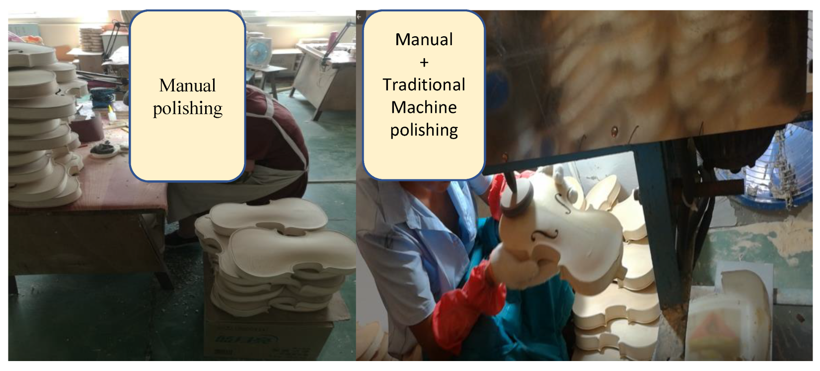
5.1. Experimental Setup

Manual polishing in Figure 6 shows the traditional manual polishing methods for violin surfaces at the Finelegened company, Taizhou, China, while Figure 7 shows the proposed automatic robotic polishing setup, which is composed of software and hardware devices. Figure 8 shows the experimental setup on path1; point-0 and point-4. The software includes the Windows 7 operating system, Qt platform, UR-10 motion control, INtime system, and user diagram protocol (UDP). Which are provided by Lihang company, Nanjing, China. The UR-10 motion control contains algorithms for path planning, force control, and gravity compensation. The Qt platform graphical user interface (GUI) is for robot motion control, where the INtime system is used as a real-time methodology for this application. The hardware implementation includes the following: UR-10 manipulator, industrial computer, UR control unit, force/torque sensor (type XLH93003ACN) with 1000 N in the z-direction and accuracy of 2.3%, UDP named NET F/T, polishing tool (type S-rima), and air pressure pump source. The polishing tool has a maximum air pressure of 75 psi, no-load speed of 10,000 rpm, air tube diameter of $1/4$ in’, and mass of 600 g. The laser microscope device OLYMPUS was used to assess surface roughness before and after polishing.

The automatic polishing system is undertaking performs the following stages steps for a polishing process: (1) performing gravity compensation in real -time, (2) identifying the coordinates system $\left(xyz\right)$ of points on the work-piece, (3) generateing smooth path polishing, and (4) adjusting contact force. The connection between the industrial computer and robot control system through (TCP/IP) protocol is via Ethernet. The NET F/T connects a force sensor with an industrial computer via transmission speed reaching to 9000 Hz, which transfers the analogue force signal to a digital value and sends it to an industrial computer to compare it with the desired value. Then, the online admittance controller algorithm computes the error and compensates by correcting the force value. The polishing machine tool is linked to the end-effector after a force sensor. The Qt environment platform registers and saves control points, the gravity compensation information, force data, and generated paths. For the S-curve trajectory, the time parameters are assumed as: $T=1.25$ s, $t_0=0$, $T_a=0.5$ s, $T_d=2$ s, $h=0.25$ m. The admittance parameters were assumed as $M_r$ = 1 (N.$s^2$/m), ${\mathrm{K}}_r$= 0.6 (N/m) ${\mathrm{B}}_r$ = 40 (N.s/m), $F_d$ = (10, 15, 20)N and $X_t=0.15$ m.

The violin surface discussed in this paper is not easy to polish by the robot using traditional control methods because it includes a mixture of various surface types, such as concave, convex, and curved; for this reason, we classify it a complex surface, as shown in Figure 9. The polishing experiment was performed to show the effectiveness of an automatic system over traditional manual systems.

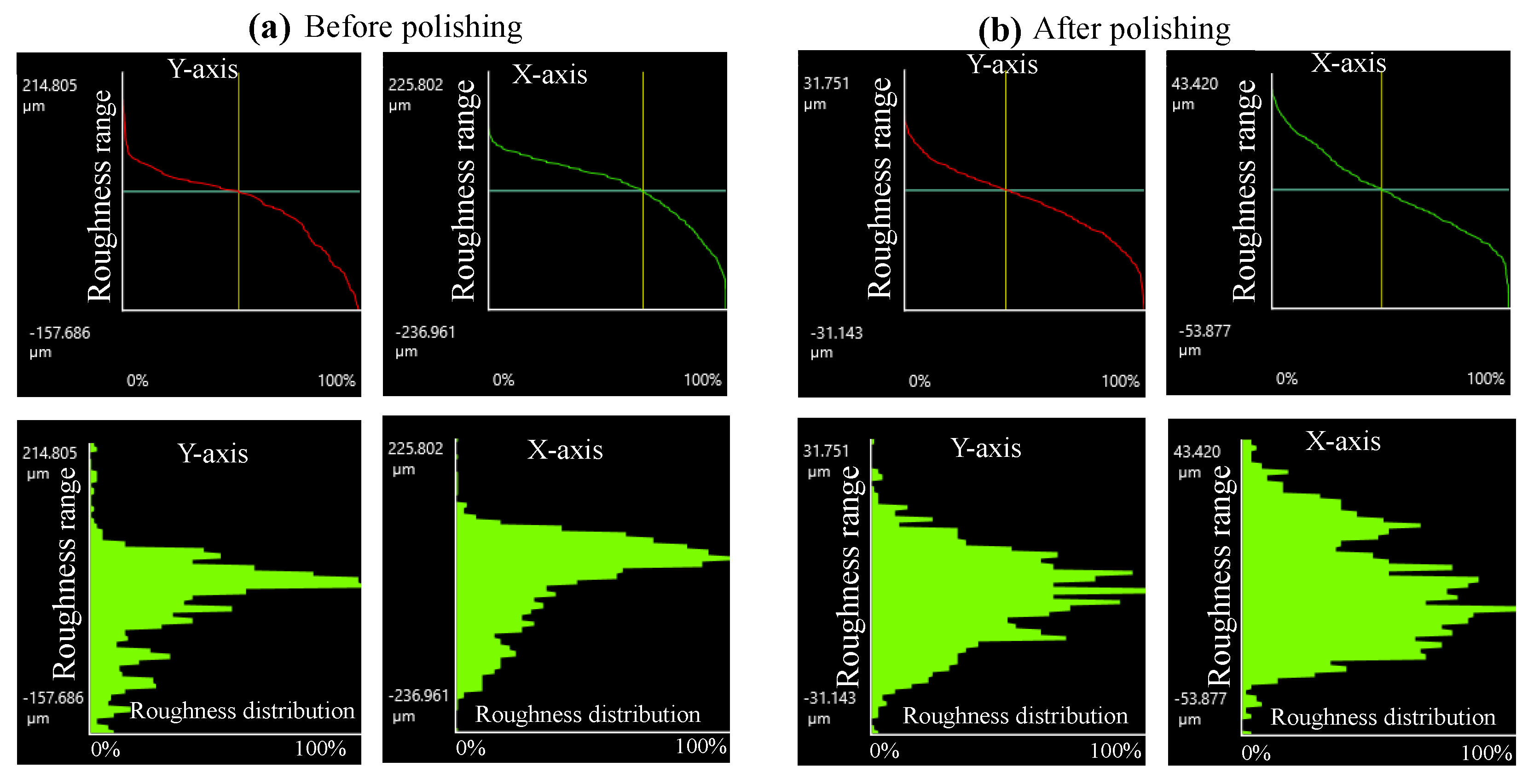
5.2. Results and Discussion

The experiment results can be described in three stages: first, showing used polishing paths and clarifying removal depths; second, explaining applied normal contact forces; and lastly, evaluating the surface roughness of the violin workpiece before and after polishing.

First, Figure 10a shows the planned control points for three polishing paths used to polish the violin surface, with eight control points for every path. Here, P01, P02, and P03 represent the first control points for path1, path2, and path3, respectively, and similarly for the other points. Figure 10b–d show the polishing paths—path1, path 2, and path 3—used to polish the violin surface. These paths had equal spacing between them to reduce the overlap between the polished areas. Based on Figure 10b–d, these paths were sufficiently smooth, which means that the proposed path-planning method achieved its aim. While Figure 11a–c, where the Figure 11b shows the material removal depth before and after polishing based on applying these forces.

Table 1. The control points (mm) on the violin surface.

Point	${\mathit{X}}_{\mathbf{curve}1}$	${\mathit{Y}}_{\mathbf{curve}1}$	${\mathit{Z}}_{\mathbf{curve}1}$	Point	${\mathit{X}}_{\mathbf{curve}2}$	${\mathit{Y}}_{\mathbf{curve}2}$	${\mathit{Z}}_{\mathbf{curve}2}$	Point	${\mathit{X}}_{\mathbf{curve}3}$	${\mathit{Y}}_{\mathbf{curve}3}$	${\mathit{Z}}_{\mathbf{curve}3}$
P01	−508.72	88.12	212.35	P02	−524.10	82.09	219.05	P03	−546.72	79.40	221.70
P11	−560.85	160.33	212.01	P12	−554.81	147.57	218.48	P13	−556.53	120.20	221.44
P21	−669.15	119.84	216.67	P22	−663.76	119.60	222.83	P23	−664.31	−99.54	226.69
P31	−749.56	141.78	212.74	P32	−773.46	129.72	219.33	P33	−767.00	115.97	221.54
P41	−815.76	84.26	213.18	P42	−794.32	82.50	220.70	P43	−764.94	84.60	223.66
P51	−762.77	19.06	211.56	P52	−764.33	31.20	217.62	P53	−750.53	54.10	222.15
P61	−680.64	38.68	214.55	P62	−668.29	45.57	220.59	P63	−7663.47	66.33	226.12
P71	−561.96	−2.43	211.79	P72	−546.95	25.30	218.13	P7	−542.65	47.62	219.74
P81	−508.72	88.12	212.52	P82	−524.10	82.09	219.05	P83	−546.72	79.40	221.70

shows the coordinates system $\left(xyz\right)$ for these paths before the polishing using our methodology through a GUI designed with Qt software. Thus, when the operator teaches the specific control point on the surface, the Qt design (GUI) can identify and save the position of this control point.

Table 2. Z-axes positions (mm) of path 1 after polished by 10, 15 and 20 N.

Point	${\mathit{Z}}_{\mathbf{curve}1}^{\prime }$	$\mathit{R}.{\mathit{d}}^{\prime }$	${\mathit{Z}}_{\mathbf{curve}1}^{″}$	$\mathit{R}.{\mathit{d}}^{″}$	${\mathit{Z}}_{\mathbf{curve}1}^{‴}$	$\mathit{R}.{\mathit{d}}^{‴}$
P01	212.11	0.24	211.87	0.36	211.15	0.72
P11	211.76	0.25	211.36	0.40	210.82	0.54
P21	216.45	0.22	216.17	0.28	215.72	0.45
P31	212.50	0.24	212.11	0.39	211.45	0.66
P41	212.92	0.26	212.50	0.42	212.04	0.46
P51	211.33	0.23	210.98	0.35	210.61	0.37
P61	214.34	0.21	213.97	0.37	213.42	0.55
P71	211.54	0.25	211.19	0.35	210.77	0.42
P81	212.26	0.26	211.90	0.36	211.30	0.60

shows the z-positions of path1 on its eight points, where $Z_{curve1}^{\prime }$, $Z_{curve1}^{″}$, and $Z_{curve1}^{‴}$ are z-coordinates of the eight points of path1 after polishing at 10, 15, and 20 N, respectively. Then, the removal depths $R.d^{\prime }$, $R.d^{″}$, and $R.d^{‴}$ were calculated by subtracting the values of z- positions as follows: ($Z_{curve1}^{\prime }-Z_{curve1}$), ($Z_{curve1}^{″}-Z_{curve1}^{\prime }$), ($Z_{curve1}^{‴}-Z_{curve1}^{″}$), respectively, where $Z_{curve1}$ could be obtained from Table 1. Figure 11a lists the depths on the eight control points of path1, which indicated the change of z-coordinates after applying different normal forces, while x- and y-coordinates did not change.

Second, Figure 11b–d show the measured results at applied normal forces at 10, 15, and 20 N. These values indicated that the proposed force controller could apply accurate contact force with some fluctuations caused by machining parameters during the polishing process. At 10 N, the fluctuation reached ±2 N; for 15 N, it reached ±3.5 N; and for 20 N, it reached ±4.8 N. Therefore, 10 N had the least fluctuation and good polishing performance. As a result, the complete polishing of this surface used this value.

Lastly, two points on the polished surface, P01 and P41 of path1, were considered to assess the surface roughness. In the laser measurement process, the middle-horizontal and vertical lines were used to show the roughness of these points in 2D, as shown in Figure 12 and Figure 13 before and after polishing for P01 and P04, respectively. The surface roughness results before polishing ranged from 201.206 to $-176.604$ $\mathsf{\mu }$m and 244.945 to $-201.950$ $\mathsf{\mu }$m for the vertical and horizontal lines, respectively, for point P01. After polishing, the surface roughness was reduced to 55.633 to $-17.755$ $\mathsf{\mu }$m and 46.40 to $-47.154$ $\mathsf{\mu }$m, respectively. For point P04, the surface roughness was 214.805 to $-157.686$ $\mathsf{\mu }$m and 255.802 to $-236.961$ $\mathsf{\mu }$m, respectively, while the roughness after polishing reduced to 31.751 to $-31.143$ $\mathsf{\mu }$m and 43.420 to $-53.877$ $\mathsf{\mu }$m, as shown in Figure 14 and Figure 15, respectively. The obtained roughness according to ISO grade, is the Roughness average (Ra) which is usually expressed in micrometers. This is the most globally known and used universal standard of roughness measuring. Figure 16 shows the experimental setup of the surface roughness measurement.

According to the overall results, we can conclude that the proposed method achieved smooth polishing paths and accurate polishing force. These achievements helped obtain equal removal depths that led to a surface roughness at the minimum required values that were suitable for the next finishing step, the painting process.

The benefits of robotic polishing compared to traditional polishing processes used in the Taizhou factory include improved quality of the polished surface. In addition, while conventional polishing reduces surface roughness from 250–200 to 90–80 µm, our robotic polishing reduced surface roughness from 250–200 to 55–30 µm. Furthermore, the operational efficiency of this workpiece is increased in the factory because the manual process cannot be reliable and accurate for extended periods, but the robot can provide these features. Moreover, decreasing the time-consumption of surface polishing is decreased. According to traditional polishing methods, the total time to polish this surface depends on the laborer’s experience. It takes around 5 min for manual pre-treatment polishing and about 5.5 min using the traditional polishing machine. However, robotic polishings complete the process in around 3.25 min. Similarly, the number of laborers in this factory can be reduced by 60%, i.e., using two robots for every room reduces the number of laborers from ten to four. Finally, the result of lowering labor production costs is also reduced.

6. Conclusions

The problem of the automatic polishing process for complex geometry parts such as violin workpieces using robotic technology was studied. An advanced mathematical model for the robotic polishing process was proposed.

Three key factors for the presented mathematical model were considered: smooth polishing path, accurate constant contact force, and material removal depth profile. The integrated NURBS and S-curve models generated a smooth polishing path. A modified admittance control law based on constant admittance control was improved based on an online environment stiffness to adapt to any complex environment. To address the contact force error, the force damping law based on force feedback by adjusting the damping parameter was studied. A simple removal depth profile model based on the Pythagorean theorem was proposed.

We conducted an experimental study to verify the feasibility of the presented methodology. The experimental results showed that the generated polishing paths were very smooth, where the overall violin surface was polished through three paths, and every path contained eight control points. In addition, an online admittance controller achieved accurate constant contact force with fluctuations reaching ±2 N, ±3.5 N, and ±4.8 N for 10, 15, and 20 N, respectively. An equal removal depth using a force of 10 N was chosen because it exhibited the least fluctuation. The surface roughness evaluation showed that the proposed polishing methodology effectively achieved the required surface roughness for the violin surface, which ranged from 55–30 $\mathsf{\mu }$m. The presented polishing strategy is valid for different surfaces, such as simple, curved, complex, and very complex, which represent challenges in the polishing process for some companies in China.

References

1. Li, J.; Guan, Y.; Chen, H.; Wang, B.; Zhang, T.; Liu, X.; Hong, J.; Wang, D.; Zhang, H. A high-bandwidth end-effector with active force control for robotic polishing. IEEE Access 2020, 8, 169122–169135. [Google Scholar] [CrossRef]
2. Mohsin, I.; He, K.; Li, Z.; Zhang, F.; Du, R. Optimization of the polishing efficiency and torque by using Taguchi method and ANOVA in robotic polishing. Appl. Sci. 2020, 10, 824. [Google Scholar] [CrossRef] [Green Version]
3. Xie, X.; Sun, L. Force control based robotic grinding system and application. In Proceedings of the 2016 12th World Congress on Intelligent Control and Automation (WCICA), Guilin, China, 12–15 June 2016; pp. 2552–2555. [Google Scholar]
4. Lin, W.; Xu, P.; Li, B.; Yang, X. Path planning of mechanical polishing process for freeform surface with a small polishing tool. Robot. Biomim. 2014, 1, 24. [Google Scholar] [CrossRef] [Green Version]
5. yczkowska-Widłak, E.; Lochyński, P.; Nawrat, G. Electrochemical polishing of austenitic stainless steels. Materials 2020, 13, 2557. [Google Scholar] [CrossRef] [PubMed]
6. Mohammad, A.E.K.; Hong, J.; Wang, D.; Guan, Y. Synergistic integrated design of an electrochemical mechanical polishing end-effector for robotic polishing applications. Robot. Comput.-Integr. Manuf. 2019, 55, 65–75. [Google Scholar]
7. Cui, Z.; Meng, F.; Liang, Y.; Zhang, C.; Wang, Z.; Qu, S.; Yu, T.; Zhao, J. Sub-regional polishing and machining trajectory selection of complex surface based on K9 optical glass. J. Mater. Process. Technol. 2022, 304, 117563. [Google Scholar] [CrossRef]
8. Su, J.B.; Liao, H.Y.; Su, Q.S. The current status and development trend in research of robotic polishing system for die and mould. Moju Gongye (Die Mould. Ind.) 2012, 38, 63–66. [Google Scholar]
9. Tian, F.; Lv, C.; Li, Z.; Liu, G. Modeling and control of robotic automatic polishing for curved surfaces. CIRP J. Manuf. Sci. Technol. 2016, 14, 55–64. [Google Scholar] [CrossRef]
10. Feng, D.; Sun, Y.; Du, H. Investigations on the automatic precision polishing of curved surfaces using a five-axis machining centre. Int. J. Adv. Manuf. Technol. 2014, 72, 1625–1637. [Google Scholar] [CrossRef]
11. Kalt, E.; Monfared, R.; Jackson, M. Towards an automated polishing system: Capturing manual polishing operations. Int. J. Res. Eng. Technol. 2016, 5, 182–192. [Google Scholar]
12. Liao, L.; Xi, F. A linearized model for control of automated polishing process. In Proceedings of the 2005 IEEE Conference on Control Applications, Toronto, ON, Canada, 28–31 August 2005; pp. 986–991. [Google Scholar]
13. Fan, C.; Hong, G.S.; Zhao, J.; Zhang, L.; Zhao, J.; Sun, L. The integral sliding mode control of a pneumatic force servo for the polishing process. Precis. Eng. 2019, 55, 154–170. [Google Scholar] [CrossRef]
14. Márquez, J.; Pérez, J.; Rıos, J.; Vizán, A. Process modeling for robotic polishing. J. Mater. Process. Technol. 2005, 159, 69–82. [Google Scholar] [CrossRef]
15. Kharidege, A.; Ting, D.T.; Yajun, Z. A practical approach for automated polishing system of free-form surface path generation based on industrial arm robot. Int. J. Adv. Manuf. Technol. 2017, 93, 3921–3934. [Google Scholar] [CrossRef]
16. Ye, J.; Niu, Z.; Zhang, X.; Wang, W.; Xu, M. In-situ deflectometic measurement of transparent optics in precision robotic polishing. Precis. Eng. 2020, 64, 63–69. [Google Scholar] [CrossRef]
17. Dong, J.; Shi, J.; Liu, C.; Yu, T. Research of pneumatic polishing force control system based on high speed on/off with PWM controlling. Robot. Comput.-Integr. Manuf. 2021, 70, 102133. [Google Scholar] [CrossRef]
18. Zhang, X.; Wang, W.; Chen, Y.; Xu, M. In-Situ Inspection for Robotic Polishing of Complex Optics. Int. J. Robot. Autom. Technol. 2022, 9, 26–32. [Google Scholar] [CrossRef]
19. Ge, J.; Deng, Z.; Li, Z.; Li, W.; Lv, L.; Liu, T. Robot welding seam online grinding system based on laser vision guidance. Int. J. Adv. Manuf. Technol. 2021, 116, 1737–1749. [Google Scholar] [CrossRef]
20. Li, J.; Zhang, T.; Liu, X.; Guan, Y.; Wang, D. A survey of robotic polishing. In Proceedings of the 2018 IEEE International Conference on Robotics and Biomimetics (ROBIO), Kuala Lumpur, Malaysia, 12–15 December 2018; pp. 2125–2132. [Google Scholar]
21. Zhu, D.; Feng, X.; Xu, X.; Yang, Z.; Li, W.; Yan, S.; Ding, H. Robotic grinding of complex components: A step towards efficient and intelligent machining—Challenges, solutions, and applications. Robot. Comput.-Integr. Manuf. 2020, 65, 101908. [Google Scholar] [CrossRef]
22. Mohammad, A.E.K.; Wang, D. A novel mechatronics design of an electrochemical mechanical end-effector for robotic-based surface polishing. In Proceedings of the 2015 IEEE/SICE International Symposium on System Integration (SII), Nagoya, Japan, 11–13 December 2015; pp. 127–133. [Google Scholar]
23. Xiao, G.; Huang, Y.; Yin, J. An integrated polishing method for compressor blade surfaces. Int. J. Adv. Manuf. Technol. 2017, 88, 1723–1733. [Google Scholar] [CrossRef]
24. Zhu, D.; Xu, X.; Yang, Z.; Zhuang, K.; Yan, S.; Ding, H. Analysis and assessment of robotic belt grinding mechanisms by force modeling and force control experiments. Tribol. Int. 2018, 120, 93–98. [Google Scholar] [CrossRef]
25. Lv, Y.; Peng, Z.; Qu, C.; Zhu, D. An adaptive trajectory planning algorithm for robotic belt grinding of blade leading and trailing edges based on material removal profile model. Robot. Comput.-Integr. Manuf. 2020, 66, 101987. [Google Scholar] [CrossRef]
26. Wahballa, H.; Duan, J.; Dai, Z. Constant force tracking using online stiffness and reverse damping force of variable impedance controller for robotic polishing. Int. J. Adv. Manuf. Technol. 2022, 121, 5855–5872. [Google Scholar] [CrossRef]
27. Duan, J.; Gan, Y.; Chen, M.; Dai, X. Adaptive variable impedance control for dynamic contact force tracking in uncertain environment. Robot. Auton. Syst. 2018, 102, 54–65. [Google Scholar] [CrossRef]
28. Wang, T.; Zhao, H.; Xie, Q.; Li, X.; Ding, H. A Path Planning Method Under Constant Contact Force for Robotic Belt Grinding. In Intelligent Robotics and Applications, Proceedings of the 12th International Conference, ICIRA 2019, Shenyang, China, 8–11 August 2019; Springer: Cham, Switzerland, 2019; pp. 35–49. [Google Scholar]
29. Zhang, J.; Wang, H.; Kumar, A.S.; Jin, M. Experimental and theoretical study of internal finishing by a novel magnetically driven polishing tool. Int. J. Mach. Tools Manuf. 2020, 153, 103552. [Google Scholar] [CrossRef]
30. Xiaohu, X.; Dahu, Z.; Zhang, H.; Sijie, Y.; Han, D. Application of novel force control strategies to enhance robotic abrasive belt grinding quality of aero-engine blades. Chin. J. Aeronaut. 2019, 32, 2368–2382. [Google Scholar]
31. Mohsin, I.; He, K.; Li, Z.; Du, R. Path planning under force control in robotic polishing of the complex curved surfaces. Appl. Sci. 2019, 9, 5489. [Google Scholar] [CrossRef] [Green Version]
32. Zhu, D.; Luo, S.; Yang, L.; Chen, W.; Yan, S.; Ding, H. On energetic assessment of cutting mechanisms in robot-assisted belt grinding of titanium alloys. Tribol. Int. 2015, 90, 55–59. [Google Scholar] [CrossRef]
33. Yang, Y.; Ruoqi, W.; Yingpeng, W.; Yuwen, S. Contact force controlled robotic polishing for complex PMMA parts with an active end-effector. J. Adv. Manuf. Sci. Technol. 2021, 1, 2021012. [Google Scholar]
34. Tian, F.; Li, Z.; Lv, C.; Liu, G. Polishing pressure investigations of robot automatic polishing on curved surfaces. Int. J. Adv. Manuf. Technol. 2016, 87, 639–646. [Google Scholar] [CrossRef]
35. Ding, Y.; Min, X.; Fu, W.; Liang, Z. Research and application on force control of industrial robot polishing concave curved surfaces. Proc. Inst. Mech. Eng. Part B J. Eng. Manuf. 2019, 233, 1674–1686. [Google Scholar] [CrossRef]
36. Feng-yun, L.; Tian-sheng, L. Development of a robot system for complex surfaces polishing based on CL data. Int. J. Adv. Manuf. Technol. 2005, 26, 1132–1137. [Google Scholar] [CrossRef]
37. Hähnel, S.; Pini, F.; Leali, F.; Dambon, O.; Bergs, T.; Bletek, T. Reconfigurable robotic solution for effective finishing of complex surfaces. In Proceedings of the 2018 IEEE 23rd International Conference on Emerging Technologies and Factory Automation (ETFA), Turin, Italy, 4–7 September 2018; Volume 1, pp. 1285–1290. [Google Scholar]
38. Huang, T.; Li, C.; Wang, Z.; Liu, Y.; Chen, G. A flexible system of complex surface polishing based on the analysis of the contact force and path research. In Proceedings of the 2016 IEEE Workshop on Advanced Robotics and Its Social Impacts (ARSO), Shanghai, China, 8–10 July 2016; pp. 289–293. [Google Scholar]
39. Mohsin, I.; He, K.; Du, R. Robotic Polishing of Free-Form Surfaces with Controlled Force and Effective Path Planning. In Proceedings of the ASME International Mechanical Engineering Congress and Exposition, Pittsburgh, PA, USA, 9–15 November 2018; Volume 52064, p. V005T07A003. [Google Scholar]
40. Ochoa, H.; Cortesão, R. Impedance control architecture for robotic-assisted mold polishing based on human demonstration. IEEE Trans. Ind. Electron. 2021, 69, 3822–3830. [Google Scholar] [CrossRef]
41. Li, Y. Arc-Length Parameterized NURBS Tool Path Generation and Velocity Profile Planning for Accurate 3-Axis Curve Milling. Ph.D. Thesis, Concordia University, Montreal, QC, Canada, 2012. [Google Scholar]
42. Biagiotti, L.; Melchiorri, C. Trajectory Planning for Automatic Machines and Robots; Springer Science & Business Media: Berlin/Heidelberg, Germany, 2008. [Google Scholar]
43. Amersdorfer, M.; Kappey, J.; Meurer, T. Real-time freeform surface and path tracking for force controlled robotic tooling applications. Robot. Comput.-Integr. Manuf. 2020, 65, 101955. [Google Scholar] [CrossRef]
44. Duan, J.; Liu, Z.; Bin, Y.; Cui, K.; Dai, Z. Payload Identification and Gravity/Inertial Compensation for Six-Dimensional Force/Torque Sensor with a Fast and Robust Trajectory Design Approach. Sensors 2022, 22, 439. [Google Scholar] [CrossRef]
Figure 1. Contact force model.
Machines 11 00147 g001
Figure 2. Schematic diagram of an online admittance controller with gravity compensation.
Machines 11 00147 g002
Figure 3. Schematic diagram of gravity compensation in six-dimensional force sensor coordinate system.
Machines 11 00147 g003
Figure 4. Multi-selected points on violin surface.
Machines 11 00147 g004
Figure 5. Material removal depth on violin surface (a) z-position before polishing (b) z-position after polishing.
Machines 11 00147 g005
Figure 6. Manual polishing of violin surface.
Machines 11 00147 g006
Figure 7. Experimental setup.
Machines 11 00147 g007
Figure 8. Experimental setup on path 1 (a) P0 and (b) P4.
Machines 11 00147 g008
Figure 9. Violin complex surface.
Machines 11 00147 g009
Figure 10. The polishing paths (a) control points on work-piece (b) path1 , (c) path 2 and (d) path3.
Machines 11 00147 g010
Figure 11. Removal depths and polishing forces (a) removal depths at (10, 15, and 20) N (b) polishing force at 10 N, (c) polishing force at 15 N, and (d) polishing force at 20 N.
Machines 11 00147 g011
Figure 12. Surface microstructure on P01 of path1 in 2D (a) before polishing, (b) after polishing.
Machines 11 00147 g012
Figure 13. Surface microstructure on P04-path1 in 2D (a) before polishing, (b) after polishing.
Machines 11 00147 g013
Figure 14. Surface roughness analysis of P0-path1 before and after polishing.
Machines 11 00147 g014
Figure 15. Surface roughness analysis of P4-path1 before and after polishing.
Machines 11 00147 g015
Figure 16. (a) OLYMPUS laser microscope, violin surface (b) before polishing, and (c) after polishing.
Machines 11 00147 g016