A Study of Noise Effect in Electrical Machines Bearing Fault Detection and Diagnosis Considering Different Representative Feature Models

Abstract

As the field of fault diagnosis in electrical machines has significantly attracted the interest of the research community in recent years, several methods have arisen in the literature. Also, raw data signals can be acquired easily nowadays, and, thus, machine learning (ML) and deep learning (DL) are candidate tools for effective diagnosis. At the same time, a challenging task is to identify the presence and type of a bearing fault under noisy conditions, especially when relevant faults are at their incipient stage. Since, in real-world applications and especially in industrial processes, electrical machines operate in constantly noisy environments, a key to an effective approach lies in the preprocessing stage adopted. In this work, an evaluation study is conducted to find the most suitable signal preprocessing techniques and the most effective model for fault diagnosis of 16 conditions/classes, from a low-workload (computational burden) perspective using a well-known dataset. More specifically, the reliability and resiliency of conventional ML and DL models is investigated here, towards rolling bearing fault detection, simulating data that correspond to noisy industrial environments. Diverse preprocessing methods are applied in order to study the performance of different training methods from the feature extraction perspective. These feature extraction methods include statistical features in time-domain analysis (TDA); wavelet packet decomposition (WPD); continuous wavelet transform (CWT); and signal-to-image conversion (SIC), utilizing raw vibration signals acquired under varying load conditions. The noise effect is examined and thoroughly commented on. Finally, the paper provides accumulated usual practices in the sense of preferred preprocessing methods and training models under different load and noise conditions.

1. Introduction

Rolling bearings are essential components of rotating machinery with considerable importance in the problem of fault detection and diagnosis, accounting for one-third of the total defects in induction machine failures [1]. The quality and performance of these indispensable parts directly affect the reliability, efficiency and down-time of electrical machines. Four main faults can occur in bearings, namely, inner race; outer race; ball or rolling element; and cage, under variable and high loads, resulting in economic costs and even safety accidents in case of escalation. Fault detection and diagnosis in rolling bearings have been widely studied using model-based methods [2], signal processing approaches [3] and data-driven techniques [4]. Developing a mathematical model of bearing faults is not always feasible, especially in complex dynamic systems. The continuously increasing availability of data has led the research focus on data-driven techniques. Knowledge is extracted incorporating feature engineering processes on raw data acquired from diverse sensor measurements. These sensing modalities include the following [5]: stator current measurements, vibration signals, sound or acoustic emission signals, and thermal analysis. Major efforts are needed to establish a real-world testbed to collect measurements from bearing faults of different types. Fortunately, different organizations publicly provide such bearing fault datasets, that contain individual stator current signals, vibration signals or both. For example, the most popular bearing fault datasets among them are CWRU [6], IMS [7], Paderborn university [8] and PRONOSTIA [9]. These bearing datasets are used as a standard reference since they are essential for validating the performance of different models and approaches in the field of fault detection and diagnosis.

Conventional signal processing techniques for rolling-element bearing fault detection using vibration signals include time-domain [10], frequency-domain [11] and time–frequency-domain analysis [12]. In time-domain analysis, characteristic features of signal statistics are calculated using temporal vibrational signal data. These features include root mean square (RMS), peak value, peak-to-peak value, skewness, kurtosis, crest factor, form factor, standard deviation and min–max values [13]. The time-domain vibration signals can be converted to frequency components using fast Fourier transform (FFT). Thus, FFT and discrete Fourier transform (DFT), spectrum analysis and envelope analysis are the most common frequency domain candidates detecting the required specific frequency components [14,15]. In time-frequency domain analysis there is a combination of both time and frequency domains using approaches like short-time Fourier transform (STFT) [16], wavelet analysis (continuous wavelet transform—CWT, discrete wavelet transform—DWT) [17,18], wavelet packet decomposition [19], empirical mode decomposition [20], variational mode decomposition [21], Hilbert transform [22] and stochastic resonance [23].

There is a long list of machine learning (ML) and deep learning (DL) methods that are utilized in the rolling bearing fault diagnosis domain [17]. ML approaches find patterns in the extracted features producing predictions of bearing fault types. On the other hand, DL methods incorporate processes that enable feature extraction in an automatic manner, learn high-level features in their hidden layers and classify fault types. However, as the availability of data increases then the performance produced by DL techniques can be significantly enhanced compared with standard ML models. Indicative ML-based approaches that have been reported in the literature for bearing fault detection are support vector machine (SVM) [24], k-nearest neighbor (k-NN) [25], principal component analysis (PCA) [26], singular value decomposition (SVD) [27] and fuzzy cognitive networks with functional weights (FCN-FW) [28]. Approaches of particular importance are those that are based on optimization methods such as particle swarm optimization (PSO) [29], mayfly optimization algorithm (MMA) [30], whale optimization algorithm (WOA) and gray wolf optimization (GWO) [31]. Broadly practiced DL implementations in the application under examination are as follows: convolutional neural networks (CNNs) [32,33]; auto-encoders (AEs) [34,35]; deep belief networks (DBNs) [36]; recurrent neural networks (RNNs) [37]; long short-term memory (LSTM) [38]; and generative adversarial networks (GANs) [39]. This class of models can deal with 1D signals, as well as 2D images that have been converted from the raw vibration signal or a feature extraction method such as continuous wavelet transform.

A challenging task is to identify the presence and type of a bearing fault under noisy conditions, especially when faults are at their incipient stage. In real-world applications and especially in industrial processes, electrical machines operate in constantly noisy environments. The background noise is an inherent characteristic in industrial sites and practically unavoidable. In the case of rolling bearings, the acquired vibration signals may contain a level of noise due to lack of lubrication, improper installation, imprecise manufacturing, high rotational speed or vibration caused by other parts of the machine. For this reason, denoising methods have been proposed to remove the noisy part from vibration signals [40], but prior and expert knowledge is required often [41]. Deep learning has attracted increasing interest in recent years for its use in bearing fault diagnosis in noisy environments. Different implementations have been presented in the literature aiming to propose an accurate learning model to detect such faults in noisy environments [42,43,44,45].

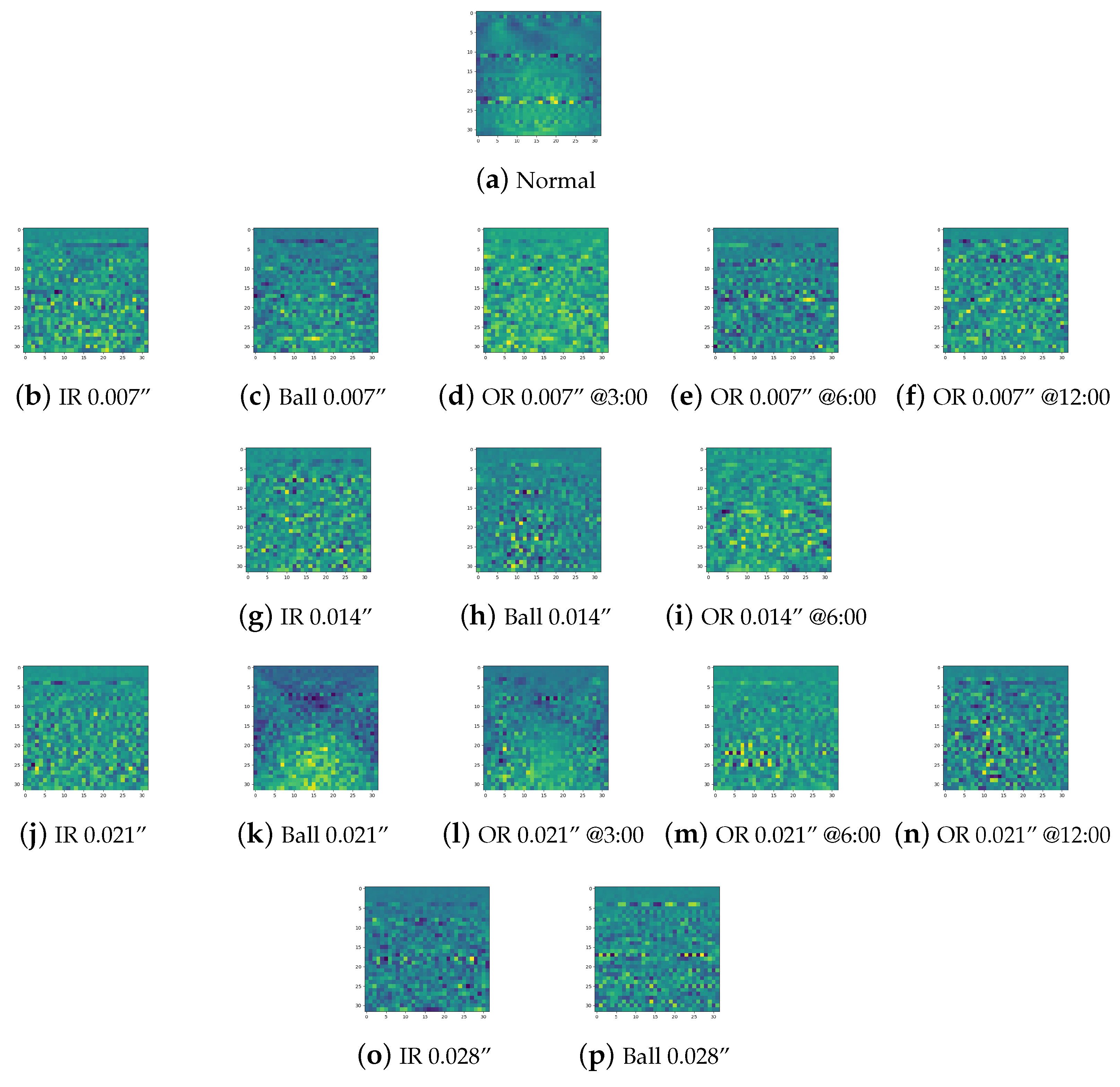
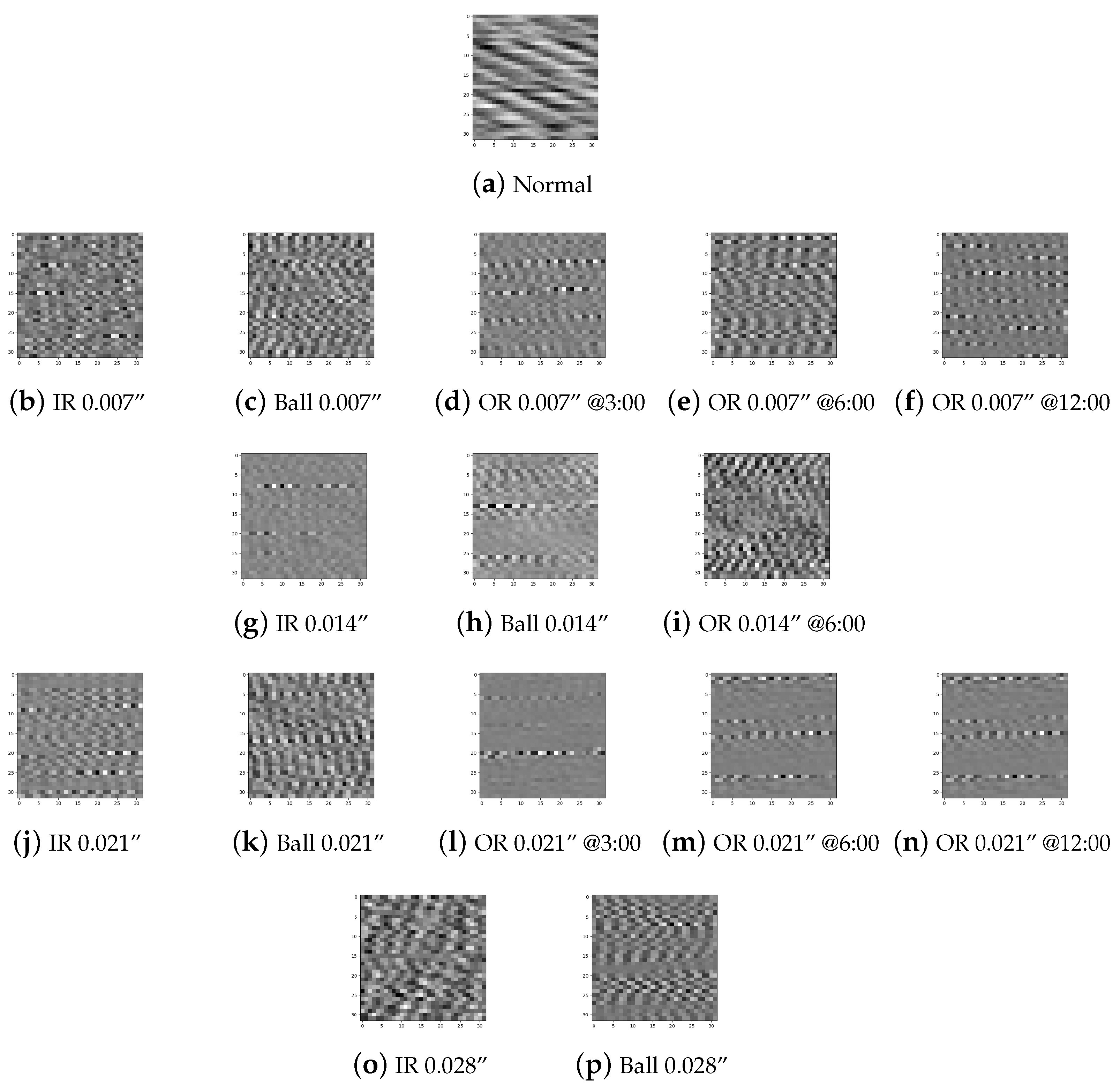
The subject of this work is evaluating different conventional learning models utilizing different preprocessing methods. Also, this work is aligned with a low-cost orientation and, therefore, evaluations are made on the 12 kHz of the CWRU dataset taking into account the total number of trainable parameters. For example, instead of using large segments of 1D vibration signals to produce larger images as inputs to the learning models and subsequently aim at higher overall performance, we study the performance of all adopted learning approaches from the preprocessing perspective under more feasible computational workloads. More specifically, in this work we investigate the reliability and resiliency of conventional ML and DL models towards rolling bearing fault detection, simulating data that correspond to noisy industrial environments. Diverse preprocessing methods have been applied in order to study the performance of SVM, Lenet-5, 1D-CNN and 2D-CNN from the feature extraction perspective. These feature extraction methods include statistical features in time-domain analysis (TDA); wavelet packet decomposition (WPD); and continuous wavelet transform (CWT); signal-to-image conversion (SIC), utilizing raw vibration signals acquired under varying load conditions of a 2 Hp induction motor with a sampling frequency of 12 kHz, as mentioned.

The paper is organized as follows: Section 2 presents, in a brief and comprehensive manner, a review of the bearing fault detection problem from basic notions and theoretical background to the main diagnostic workflow needed, embodying feature extraction methods and learning models. Section 3 is devoted to the development of the adopted implementations, as well as to their evaluation in different simulated noise environments. Section 4 covers the comparison of different cases, in terms of preprocessing methods as well as different learning models, in the bearing fault detection problem. Section 5 provides an analytical discussion of the conducted study, while conclusions are given in Section 6.

2. Bearing Fault Detection Workflow, Problem Description and Review

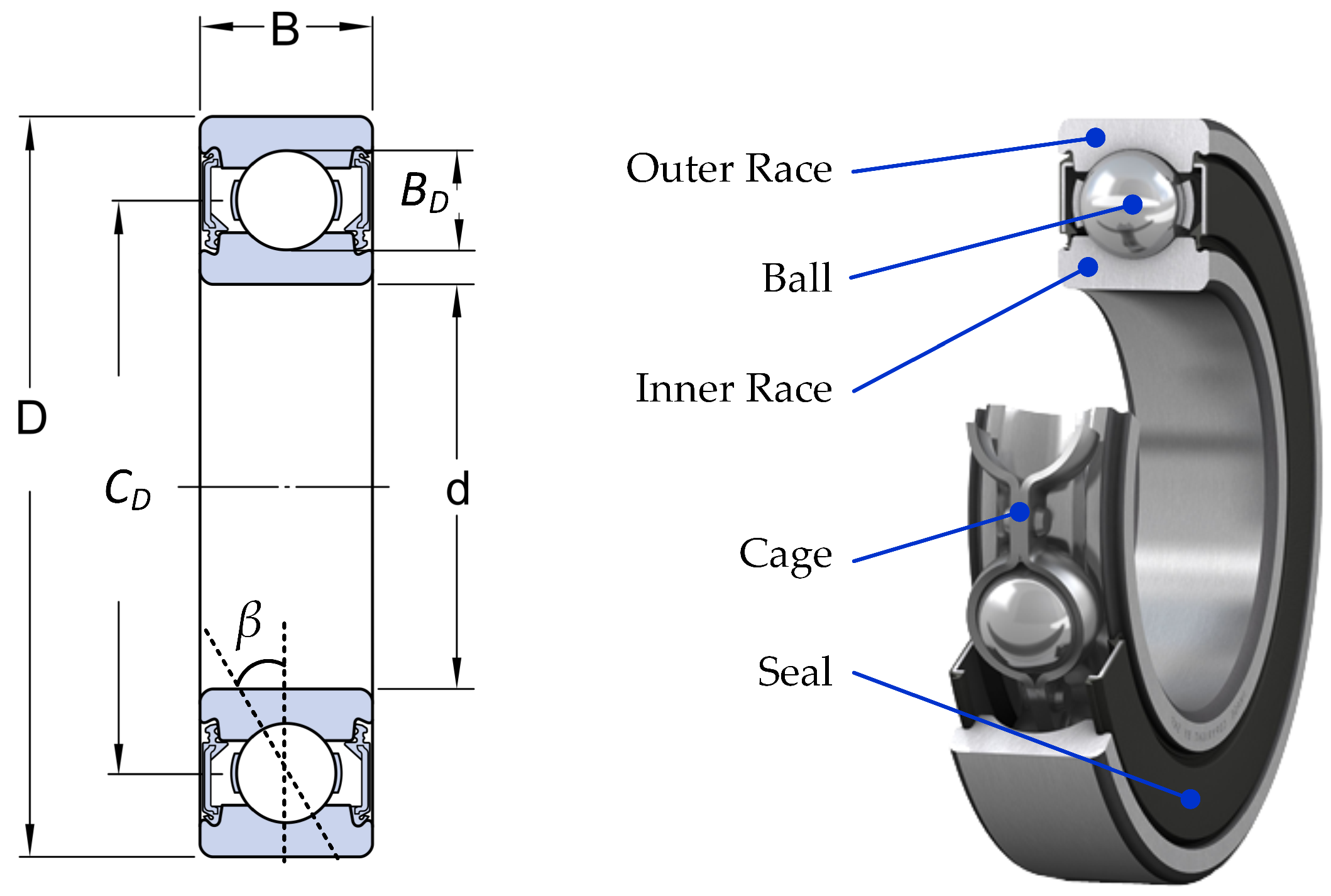
Various parts of a rotating electrical machine, such as the stator, rotor and rolling bearings, are susceptible to significant issues [46]. Notably, rolling bearing defects are among the most frequent types of failures in electrical motors, occurring at a rate of 30–40%. As the component that secures the rotor’s appropriate rotation from the machine shaft and serves as a mechanical connection point of the electric motor, bearings are crucial to the lifespan of an electrical machine. The rolling balls, the inner and outer races and the cage, which keeps the distance between the balls equal, are just a few of the components that make up Figure 1, which illustrates a typical geometry of a rolling bearing.

Furthermore, bearing faults are caused by a variety of factors like insufficient lubrication, misalignment of rotor and mechanical stress. Each kind of bearing fault produces a pulse in the frequency spectrum, which is known as the bearing characteristic frequency. The frequencies for ball fault ($f_{bf}$), inner race fault ($f_{irf}$), outer race fault ($f_{orf}$) and cage fault ($f_c$), respectively, can be mathematically described by the following equations:

$$f_{bf}=\frac{C_D}{B_D}{f}_r\left(1-\frac{B_D^2}{C_D^2}co{s}^2\beta \right)$$

(1)

$$f_{irf}=\frac{N_b}{2}{f}_r\left(1+\frac{B_D}{C_D}cos\beta \right)$$

(2)

$$f_{orf}=\frac{N_b}{2}{f}_r\left(1-\frac{B_D}{C_D}cos\beta \right)$$

(3)

$$f_c=\frac{f_r}{2}\left(1-\frac{B_D}{C_D}cos\beta \right)$$

(4)

where $B_D$ is the ball diameter, $C_D$ is the pitch diameter, $\beta$ is the contact angle of the ball with the rails, $N_b$ is the number of rolling bearing balls and $f_r$ is the rotor frequency [47].

2.1. General Perception of the Bearing Fault Detection Workflow

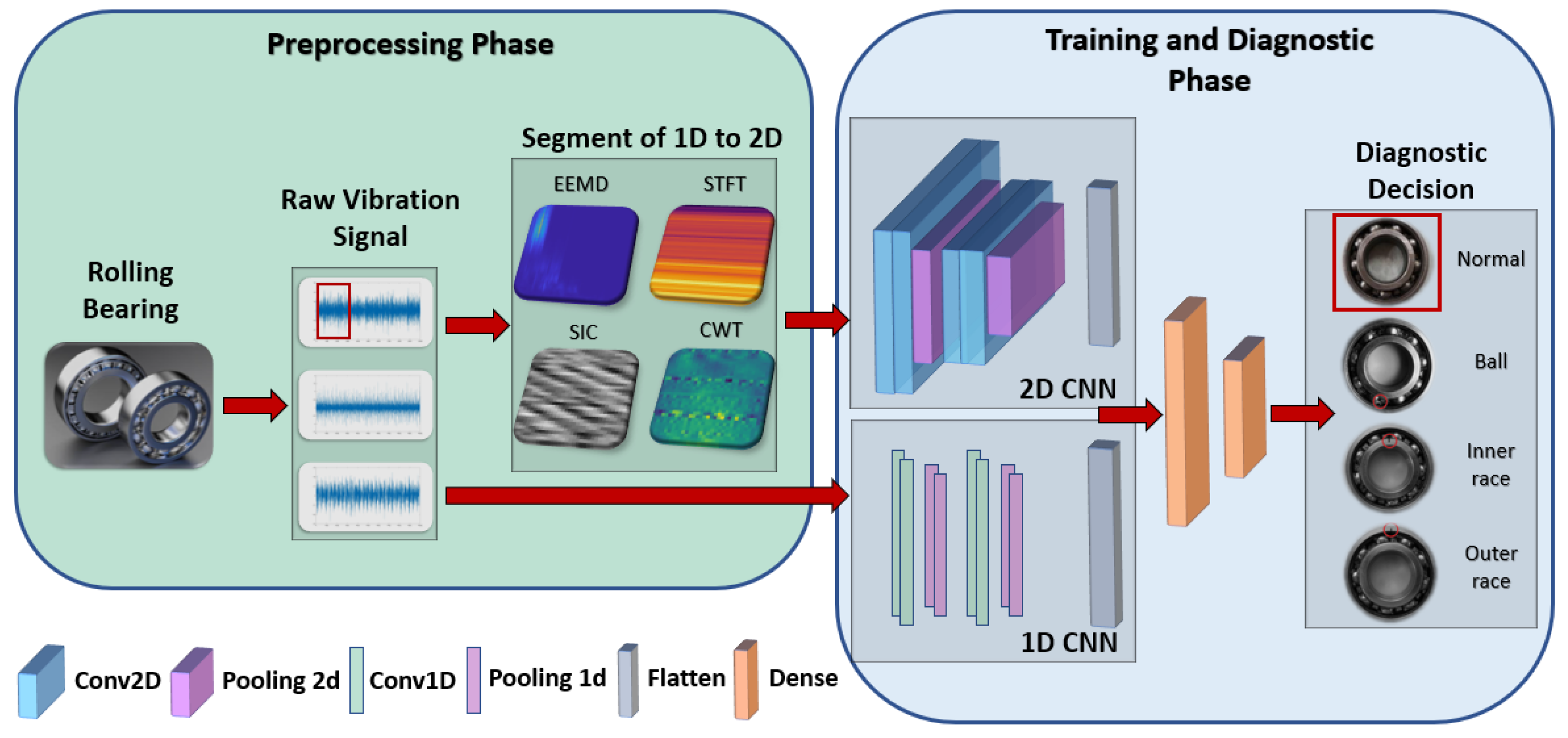
The general working procedure towards bearing fault detection involves different operational stages such as data acquisition, preprocessing, feature extraction and selection, learning mechanism and finally diagnostic decision. In a preparatory stage, a set of sensors is required to be placed at specific locations of the machine under examination. Usually, vibration data are collected, and then a preprocessing stage is applied to extract features of different domains and textures. Traditionally, the most used feature extraction methods include short-time Fourier transform (STFT), empirical mode decomposition or an extension like ensemble empirical mode decomposition (EEMD), continuous wavelet transform (CWT), signal-to-image conversion (SIC) or statistical methods. The latter provides the most compressed representation of the original signal leading to the strict utilization of machine learning approaches. Training mechanisms that incorporate deep neural learning algorithms utilize either 1D raw vibration signals or 2D representations that are produced by the aforementioned feature extraction processes. Convolutional neural network (CNN) architectures are widely used for signal processing and especially fault detection, extracting potential features encapsulated in signals and detecting local information during training. Figure 2 illustrates the general flow procedure for bearing fault detection adopting either 1D or 2D CNN as training candidate algorithms under different feature extraction methods.

2.2. A Short Review of Bearing Fault Datasets

One of the most challenging tasks in the Artificial Intelligence universe is the existence of descriptive and coherent benchmark datasets. Often, in large-scale datasets, there is the need for multidisciplinary perspectives to ensure the creation of a flawless dataset, under specific conditions and parameters, that is a reliable solution to be utilized towards solving a real-world problem. This process is consequently even more ambitious in the case of electrical machines and bearing faults. This stems from the fact that degradation occurs gradually over a long operating horizon passing from incipient stages and malfunctions towards severe conditions and eventually total degradation.

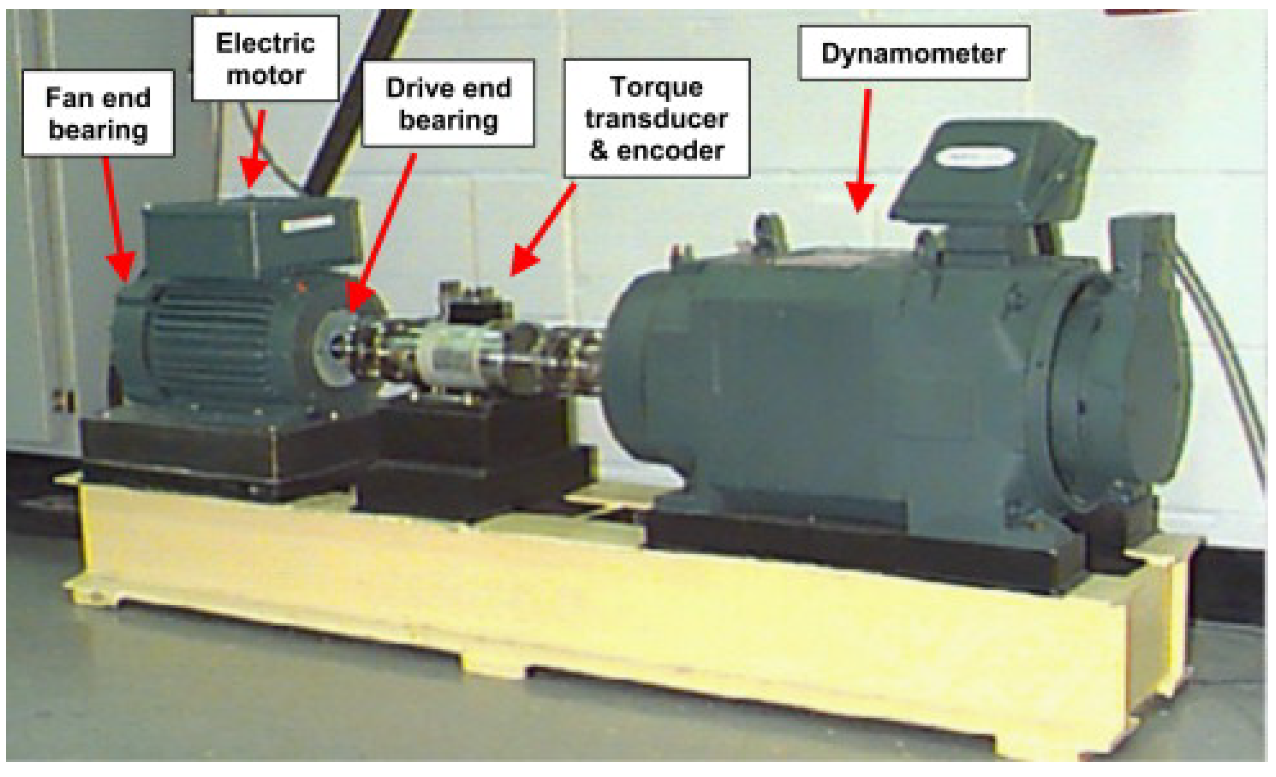
For this reason, a usual practice for data collection is to either include artificially induced faults or perform testing methods that accelerate the life-cycle of components. Apart from being time consuming, this process is prohibitively expensive and requires expert assistance to ensure that all intermediate fault states have been acquired smoothly and accurately. The following are well-known bearing fault datasets that are publicly available from different organizations: (a) Case Western Reserve University (CWRU) bearing dataset (https://engineering.case.edu/bearingdatacenter (accessed on 1 July 2023)); (b) Intelligent Maintenance Systems (IMS) (https://www.nasa.gov/content/prognostics-center-of-excellence-data-set-repository (accessed on 1 July 2023)); (c) Paderborn university bearing dataset (https://mb.uni-paderborn.de/kat/forschung/ (accessed on 1 July 2023)); and (d) IEEE PHM 2012 Prognostic Challenge (PRONOSTIA). A brief comparison of the aforementioned datasets is presented in

Table 1. Description of well-known rolling bearing fault datasets.

Dataset Name	Fault Mode	Sensor Type	Sampling Rate	Fault Type
CWRU [6]	Artificial	Accelerometer (2 sensors)	12/48 kHz	Inner and outer race, ball fault; 4 fault diameters: 0.007, 0.014, 0.021 and 0.028 inches; 4 load conditions: 0, 1, 2 and 3 (HP)
IMS [7]	Accelerated aging test	Accelerometer (2 sensors)	20 kHz	Inner and outer race, ball fault; 3 run-to-failure tests
Paderborn [8]	Artificial and Accelerated aging test	Accelerometer (1 sensor), Current (2 sensors), Thermocouple (1 sensor)	64 kHz	6 undamaged bearings and 12 artificially damaged; 14 bearing faults emerged from accelerated life tests; inner and outer race fault
PRONOSTIA [9]	Accelerated aging tests	Accelerometer (2 sensors), Thermocouple (1 sensor)	25.6 kHz	3 operating conditions; 17 run-to-failure tests

, illustrating the differences among fault mode, sensor type, sampling frequency and fault type. Note that the PRONOSTIA and IMS datasets are preferred for use in remaining useful life (RUL) prediction problems [48,49].

2.3. Feature Extraction and Selection

Diverse signal processing methods can be applied to obtain the required useful information from vibration data. These methods may vary between time-domain, frequency-domain and time–frequency-domain analysis [50]. A comprehensive review that presents the signal processing techniques utilized in the rolling element bearings fault detection area is presented in [51]. For example, the most common approaches are (a) time domain or temporal analysis—statistical features; (b) frequency domain—fast Fourier transform (FFT), power spectrum, cepstrum, envelope spectrum; (c) time–frequency domain techniques—short-time Fourier transform (STFT), wavelet based approaches like continuous wavelet transform (CWT), discrete wavelet transform (DWT), wavelet packet transform (WPT) and tunable Q-factor wavelet transform (TQWT), also empirical mode decomposition (EMD) and its extensions, and empirical wavelet transform (EWT) and morphological filter.

Feature selection is a usual practice during preprocessing in order to divide attributes into informative, redundant or irrelevant ones. This operation reduces the feature vector dimension keeping the most related and important features, while also removing the redundant and irrelevant features, avoiding overfitting and alleviating the workload. Different feature selection strategies have been proposed in the literature to choose the most discriminant features using the CWRU dataset. For example, there are approaches that are based on particle swarm optimization (PSO) [52], principal component analysis (PCA) [53] or conventional search of the feature space by greedy methods [54].

2.4. Machine Learning and Deep Learning Models

In the field of fault detection and diagnosis in electrical machines, machine learning algorithms play a crucial role offering data-driven approaches for identifying anomalies, malfunctions, degradation levels and defects. These models are trained to recognize patterns associated with normal and faulty behavior based on historical data. Feature extraction and feature engineering are essential steps in preparing the data for training machine learning models in fault detection. They involve transforming raw data into meaningful and informative features that capture relevant patterns and characteristics related to the fault type. However, these preprocessing steps may involve complex feature engineering approaches or may require domain-related expertise. Machine learning approaches that have been reported in the literature regarding bearing fault detection include mainly artificial neural networks (ANNs) [55], support vector machines (SVMs) [56] and k-nearest neighbor (KNN) [57].

Consequently, deep learning algorithms with automated feature extraction capabilities have gained popularity in bearing fault diagnostics. Deep learning is a subset of machine learning that excels in representing the problem under examination through nested hierarchies of concepts. The transition from classical machine learning to deep learning is driven by factors such as data explosion, algorithm evolution and hardware advancements. The advantages of deep learning over conventional machine learning include better performance, automatic feature extraction and transferability to different domains. As a result, deep learning has witnessed exponential growth in applications, including machine health monitoring and fault diagnostics, with bearing fault detection being a prominent example. Indicative methodologies include auto-encoder implementations [58], 2D CNN structures [59], 1D CNN classifier [60], deep belief network (DBN) [61] and attention mechanism [62]. Extensive review studies have been reported in the literature regarding the field of bearing fault detection from the scope of learning models [63,64,65].

3. Study of the Noise Effect in Bearing Fault Detection

3.1. Emulation of Different Noisy Environments

Noise in real-world applications is inevitable due to a wide range of factors that affect industrial machines: (a) inaccuracies in manufacturing and/or improper installation; (b) high rotating speed; (c) lack of lubrication in rolling bearings; (d) fluctuations in rotating parts or processes; and (e) vibration caused by other mechanical components, such as gears, blades, other bearings and rotors. However, measuring noise is a crucial step in assessing and addressing the noise generated by industrial systems. It is an essential part of noise control and management. Measuring and monitoring noise levels is important in evaluating the effectiveness of noise reduction measures and ensuring compliance with noise regulations. The choice of noise type depends on the specific application and the characteristics of the noise that need to be represented accurately. Different types of noise may be used to better match the noise sources and conditions encountered in a given domain. Additive white Gaussian noise (AWGN) is a common practice to generate different levels of noisy environments mimicking the effect of such operations. This is a preferred choice for simulating noisy environments and testing signal processing algorithms in bearing fault analysis due to its simplicity and versatility. This type of noise is well-understood and characterized by a uniform distribution of energy across all frequencies (flat power spectral density, i.e., equal intensity at all frequencies). Its straightforward mathematical properties make it an advantageous option when developing and evaluating signal processing techniques. Moreover, AWGN is often used as a baseline model for assessing algorithm performance. This choice provides a clear reference point, enabling researchers to evaluate algorithms under controlled conditions and establish a foundation for further analysis.

In bearing fault analysis, the main emphasis typically centers on the vibrational signals produced by the bearing and its components. AWGN remains a valuable tool for evaluating how algorithms respond to random, wide-band noise. This noise type can effectively replicate the background noise present in real-world industrial and mechanical settings, helping researchers test the robustness of their signal processing methods. However, in specific cases, and especially when examining rare or unusual bearing fault scenarios, color noise or Poisson noise may be more appropriate. These types of noise can help capture specific characteristics of noise sources that AWGN cannot represent accurately. Moreover, color or Poisson noise may be better in capturing the dynamic nature of industrial environments in the sense of simulating non-stationary conditions, but there are no widely specified levels reported in detail in the research works representing them as more accurate than AWGN.

On the other hand, the AWGN is independent of the characteristics of the analyzed signal and offers a generic mapping of different noisy situations without the need to know beforehand the specific properties of the signal. In this work we use 16 operational cases which stem from 4 main operational cases (normal, ball, inner and outer). If the objective of this work was related to rare and unusual bearing fault scenarios under specific conditions (like examining cases that stem solely from lack of lubrication or vibration caused in other components), then Poisson noise and more appropriately color noise would have been considered. Thus, in order to study the wide-band noise impact from an aggregated point view and estimate the capability of different models in real-world situations, we generated noisy signals by adding AWGN. The produced signals are proportional to the clean (meaningful) signal based on signal-to-noise ratio (SNR). The ratio of the power of the clean signal to the power of the background noise is denoted in the decibel form as follows:

$$SN{R}_{dB}=10{log}_{10}\left(\frac{P_{signal}}{P_{noise}}\right)$$

(5)

where the power of the original and the emulated signal is indicated as $P_{signal}$ and $P_{noise}$, respectively. Thus, we simulated five levels of noisy signals with SNR between −2 and 15 dB. More specifically, the noisy cases under investigation are as follows: (a) SNR = −2 dB; (b) SNR = 2 dB; (c) SNR = 4 dB; (d) SNR = 10 dB; and (e) SNR = 15 dB. For example, SNR = −2 dB means that noise power is 1.58 times greater than clean signal power and SNR = 15 dB means that the signal is 31.62 times more powerful than the noisy signal. However, it is important to define whether the specified noise levels are aligned with the noise interference conditions in real-life testing. In general, simulated noise signal with negative ($-2$ dB), slightly positive (up to 4 dB) and positive (5∼15 dB) values of SNR indicate strong, medium and weak noise conditions, respectively, in this application [45,66,67]. In this work, we perform an evaluation study of the noise effect in rolling bearing fault detection, emulating different noisy environments, following the noise levels utilized in [68].

3.2. Dataset under Consideration

The CWRU dataset is an open-source and widely used benchmark dataset for studying the health of rotating machinery. It is provided by the Department of Mechanical Engineering at Case Western Reserve University and contains vibration signals of four different bearing conditions: normal, inner race fault, outer race fault and ball fault. Data have been collected from an induction motor under different loading conditions (0 Hp, 1 Hp, 2 Hp and 3 Hp) within a speed range of 1797 to 1730 rpm (1797, 1772, 1750 and 1730), respectively. The experiment setup shown in Figure 3 consists of a 2 Hp induction motor, a dynamometer, a torque transducer and control electronics which are not depicted. Data collection was carried out using accelerometers attached to the housing with magnetic bases. Accelerometers were located at the 12 o’clock position on both drive end and fan end of the motor. Additionally, a 16 DAT recorder was used in order to collect the vibration signals and two sampling frequencies of 12 kHz and 48 kHz were used as well.

In this work, we choose to encapsulate all 16 bearing conditions of the CWRU dataset, as presented in

Table 2. CWRU dataset description.

Class	Fault Type	Fault Diameter (inch)
0	Ball	0.007
1	Ball	0.014
2	Ball	0.021
3	Ball	0.028
4	Inner	0.007
5	Inner	0.014
6	Inner	0.021
7	Inner	0.028
8	Outer@3.00	0.007
9	Outer@6.00	0.007
10	Outer@12.00	0.007
11	Outer@6.00	0.014
12	Outer@3.00	0.021
13	Outer@6.00	0.021
14	Outer@12.00	0.021
15	Normal	-

, for the evaluation study under examination. The 12 kHz drive end data provide a database including 16 different bearing conditions at four different fault diameters. The overall dataset consists of healthy condition, ball fault, inner race fault and outer race fault with artificially induced faults (see Table 1) including cases under four different diameters: 0.007, 0.014, 0.021 and 0.028 inches. The diameters of ball and inner race faults are as stated above, whereas the diameters of outer race faults can reach a maximum value of 0.021 inches. More precisely, the outer race faults are divided into three categories: “Centered” (6 o’clock position), “Orthogonal” (3 o’clock position) and “Opposite” (12 o’clock position). Subsequently, the vibration data were postprocessed in a Matlab environment and each one of the faulty conditions was saved in a .mat file together with the speed level, drive end and fan end data.

3.3. Adopted Feature Domains for Evaluation

In the domain of fault detection and diagnosis for electrical machines, feature extraction and signal processing play a pivotal role in enabling effective and precise health monitoring, especially when dealing with rolling bearing faults [69]. By leveraging sophisticated feature extraction and signal processing techniques, essential information is extracted from vibration and acceleration signals. Vibration signals are invaluable in a variety of engineering applications as they provide crucial insights into the condition monitoring and fault diagnosis of mechanical systems. These types of signals, typically recorded by accelerometers, capture the dynamic behavior of rotating machinery. However, raw vibration signals are often complex and rich in information, making direct interpretation challenging. The CWRU dataset contains vibration signals collected from different bearing faults under various operating conditions. Figure 4 presents, for example, the amplitude/time diagram acquired from the drive end data with a frequency range of 12 kHz for each of the 16 different bearing conditions. As illustrated, each health status has a unique vibration signal signature, taking different amplitude values for each bearing condition. The following signals serve as critical inputs for our survey, and enable us to examine the performance and the efficacy of our proposed models.

3.3.1. Statistical Features

Statistical features based on either time-domain or frequency-domain analysis can be extracted to identify bearing faults with minimum preprocessing effort and computational complexity. This is a simple and less time consuming method to extract knowledge feeding classifiers with information from an oversight perspective. The most dominant features in the frequency domain are root mean square frequency (RMSF), root variance frequency (RVF) and frequency center (FC). However, in this work we use solely the time-domain analysis (TDA) features that are presented in

Table 3. Time-domain analysis (TDA) features.

Name	Formula
min value	$min{\left\{x_i\right\}}_{i=1}^N$
max value	$max{\left\{x_i\right\}}_{i=1}^N$
mean value	$\overline{x}=\frac{{\sum }_{i=1}^N{x}_i}{N}$
standard deviation value	$\sigma =\sqrt{\frac{1}{N}{\sum }_{i=1}^N{(x_i-\overline{x})}^2}$
root mean square value	$rms={\left(\frac{1}{N}{\sum }_{i=1}^N{x}_i^2\right)}^{1/2}$
skewness value	$skewness=\frac{1}{N}{\sum }_{i=1}^N{\left[\frac{(x_i-\overline{x})}{\sigma }\right]}^3$
kurtosis value	$kurtosis=\frac{1}{N}{\sum }_{i=1}^N{\left[\frac{(x_i-\overline{x})}{\sigma }\right]}^4-3$
crest factor	$crest=\frac{max\left(x_i\right)}{{\left(\frac{1}{N}{\sum }_{i=1}^N{x}_i^2\right)}^{1/2}}$
form factor	$form=\frac{{\left(\frac{1}{N}{\sum }_{i=1}^N{x}_i^2\right)}^{1/2}}{\overline{x}}$

.

3.3.2. Wavelet Packet Decomposition

Wavelet packet decomposition (WPD) is a generalized form of discrete wavelet transform (DWT), where the 1D time-domain vibration signal is filtered using low-pass and high-pass filters. The two filters are related to each other; thus, they are both named quadratic mirror filters. Their cut-off frequency is one fourth of the sampling frequency signal. The output from the high-pass filter gives the detail coefficients (D), while the low-pass side gives the approximation coefficients (A). Both types of coefficients hold half of the original signal representing the high and low frequency content of the signal. If the decomposition continues further, then the new level (second level) will consist of four signals (each is one fourth of the original) named approximation of the approximation (AA), detail of the approximation (DA), approximation of the detail (AD) and detail of the detail (DD). In this work we use a tree depth of 3 (decomposition level); hence, the three level signals that represent the frequency content of the original signal within the bands $0-f_s/16$, $f_s/16-f_s/8$, $f_s/8-3f_s/16$, $3f_s/16-f_s/4$, $f_s/4-5f_s/16$, $5f_s/16-3f_s/8$, $3f_s/8-7f_s/16$ and $7f_s/16-f_s/2$ are named AAA, DAA, ADA, DDA, AAD, DAD, ADD and DDD. Note that $f_s$ is the sampling rate of the signal. Note that the schematic diagram of a WPD tree with three levels is illustrated in Figure 5. Let there be a 1D vibration signal of S number of samples. Denoting each packet or leaf node by j, and the decomposition level or tree depth as k, then there are $2^k$ leaves that are obtained, $W_{k,0},\dots ,W_{k,2^k-1}$, that span in the aforementioned bands, since here $k=3$. The energy $E_j$ of each packet j at each level k is given by the energy of the wavelet coefficients of each packet. The wavelet coefficients of each packet can be expressed as ${\mathbf{d}}_j^k=\{d_j^k\left(1\right),\dots ,d_j^k\left(n\right)\}$ with n being the number of coefficients ($n=1,\dots ,S/2^k$). Hence, the energy of each packet is denoted as follows:

$$E_j=\sum _{i=1}^n{\left[d_j^k\left(i\right)\right]}^2$$

(6)

Then, the jth wavelet packet feature is given by the following:

$$\begin{array}{c}\hfill {\rho }_j=\frac{E_j}{{\sum }_{i=1}^N{E}_j},\sum _j{\rho }_j=1\end{array}$$

(7)

where $N=2^k$ is the number of packets and $j=0,\dots ,N-1$. Since in this case we have a depth of 3, there are eight features $\left\{{\rho }_j\right|j=1,\dots ,16\}$ with ${\sum }_{j=1}^{16}{\rho }_j=1$. Other works that utilize WPD in the CWRU dataset are [70,71].

3.3.3. Continuous Wavelet Transform

Continuous wavelet transform (CWT) provides an established method for constructing a time–frequency representation of a signal with increased accurate time and frequency localization. Therefore, a signal is decomposed into wavelets, and the CWT basis functions are scaled and shifted forms of the time-localized mother wavelet. The adopted procedure includes, at first, data collection from each class in segments of length 1024. It should be noted that the input signal is a 1D vibration signal of S number of samples with $S=1024$, as mentioned in the WPD case. CWT is conducted on segments of data at 64 different scales. A set of 100 segments is gathered from each one of the 16 specified classes for each load condition, with no overlap between segments, leading to an output size of $(6400,1024)$. The continuous wavelet coefficients (CWCs) of vibration signals are calculated directly with the PyWavelets Python Package using Morlet wavelet $\psi$:

$$\psi \left(t\right)={exp}^{-t^2/2}cos\left(5t\right)$$

(8)

The wavelet transform with the wavelet $\psi$ of a signal $y\left(t\right)$ is given by the following [72]:

$$W_{\psi }^y=\frac{1}{\sqrt{c_{\psi }\left|\alpha \right|}}{\int }_{-\infty }^{\infty }y\left(t\right)\psi \left(\frac{t-b}{\alpha }\right)dt$$

(9)

where $c_{\psi }=\sqrt{\pi /\beta }$, $\alpha$ and b are the dilatation and translation parameters, respectively, and $\beta ={\omega }_0^2$ and ${\omega }_0$ are defined accordingly based on application. The final output is resized into $(6400,32,32)$ forming 6400 images in total to feed the two-dimensional neural network implementations. Figure 6 illustrates indicative CWT representations for each of the 16 health condition classes.

3.3.4. Signal-to-Image Conversion

The core idea of signal-to-image conversion is converting time-domain raw signals into images presenting an alternative preprocessing procedure [73]. For the creation of an $M\times M$ image, a segmented signal of length $M^2$ is obtained from the raw vibration signal. In this work we produce $32\times 32$ grayscale images as the segment signal is of length 1024. The values of the segmented part are expressed as $L\left(i\right)$ with $i=1,\dots ,M^2$, while the pixel strength of the converted image is denoted as $P(j,k)$ where both $j,k=1,\dots ,M$. Hence, the converted grayscale images are given by:

$$P(j,k)=round\left\{\frac{L\left(\right(j-1)\times M+k)-min\left(L\right)}{max\left(L\right)-min\left(L\right)}\times 255\right\}$$

(10)

where $round\{·\}$ stands for the rounding function and the transformation takes place within the interval $[0,255]$, presenting a grayscale image. As can be easily understood, the whole procedure offers a direct translation of 1D raw signals to 2D textured representations. This way, each bearing defect and the normal condition can be directly connected with a specific class of similar textured images without pre-defined parameters. Figure 7 presents indicative examples of this method applied in the CWRU dataset.

3.4. Adopted Learning Models and Evaluation Study

This section describes in a brief manner the selected candidates, from the machine learning and deep learning contexts, that formulate the evaluation study under diverse noisy conditions. It is to be remembered that the data under examination concern vibration signals acquired using a 12K sampling frequency under motor loads of 0, 1, 2 and 3 horsepower (HP), as described in Section 3.2. On the machine learning side, the support vector machine (SVM) has been chosen as an established and simple solution that maps data from low-dimensional space into higher feature space using kernel functions. The regularization parameter, also known as the penalty factor, C, is chosen to be equal to 10. This serves as the controlling variable of the trade-off between the maximization of the margin and the minimization of the training error. Also, the radial basis function is selected as the kernel function with a width of $\gamma =0.01$. From the deep learning domain, one-dimensional (1D) and two-dimensional (2D) versions of convolutional neural networks are selected, as well as the traditional LeNet-5 network. Starting with the conventional LeNet-5, its detailed architecture is presented in

Table 4. Architecture of the Lenet-5.

Layer No.	Layer Type	Kernel Size	Stride	Filters	Output Shape	Trainable Parameters
1	Convolution 1	$5\times 5$	1	6	$28\times 28$	156
2	Pooling 1	$2\times 2$	2	6	$14\times 14$	-
3	Convolution 2	$5\times 5$	1	16	$10\times 10$	2416
4	Pooling 2	$2\times 2$	2	16	$5\times 5$	-
5	Dense	-	-	-	120	48,120
6	Dense	-	-	-	84	10,164
7	Output	-	-	-	16	1360

, while 1D and 2D CNN extensions using different numbers of layers are presented in

Table 5. Architecture of the 1D CNN-2L.

Layer No.	Layer Type	Kernel Size	Stride	Filters	Output Shape	Trainable Parameters
1	Convolution 1	$3\times 1$	2	64	$511\times 64$	256
2	Pooling 1	$2\times 1$	2	64	$255\times 64$	-
3	Convolution 2	$3\times 1$	2	128	$127\times 128$	24,704
4	Pooling 2	$2\times 1$	2	128	$63\times 128$	-
5	Dense	-	-	-	100	806,500
6	Dense	-	-	-	50	5050
7	Output	-	-	-	16	816

,

Table 6. Architecture of the 1D CNN-4L.

Layer No.	Layer Type	Kernel Size	Stride	Filters	Output Shape	Trainable Parameters
1	Convolution 1	$3\times 1$	2	16	$511\times 16$	64
2	Pooling 1	$2\times 1$	2	16	$255\times 16$	-
3	Convolution 2	$3\times 1$	2	32	$127\times 32$	1568
4	Pooling 2	$2\times 1$	2	32	$63\times 32$	-
5	Convolution 3	$3\times 1$	2	64	$31\times 64$	6208
6	Pooling 6	$2\times 1$	2	64	$15\times 64$	-
7	Convolution 4	$3\times 1$	2	128	$7\times 128$	24,704
8	Pooling 4	$2\times 1$	2	128	$3\times 128$	-
9	Dense	-	-	-	100	38,500
10	Dense	-	-	-	50	5050
11	Output	-	-	-	16	816

,

Table 7. Architecture of the 2D CNN-2L.

Layer No.	Layer Type	Kernel Size	Stride	Filters	Output Shape	Trainable Parameters
1	Convolution 1	$3\times 3$	2	64	$16\times 16$	640
2	Pooling 1	$2\times 2$	2	64	$8\times 8$	-
3	Convolution 2	$3\times 3$	2	128	$4\times 4$	73,856
4	Pooling 2	$2\times 2$	2	128	$2\times 2$	-
5	Dense	-	-	-	100	51,300
6	Dense	-	-	-	50	5050
7	Output	-	-	-	16	816

and

Table 8. Architecture of the 2D CNN-4L.

Layer No.	Layer Type	Kernel Size	Stride	Filters	Output Shape	Trainable Parameters
1	Convolution 1	$3\times 3$	2	16	$16\times 16$	160
2	Pooling 1	$2\times 2$	2	16	$8\times 8$	-
3	Convolution 2	$3\times 3$	2	32	$4\times 4$	4640
4	Pooling 2	$2\times 2$	2	32	$2\times 2$	-
5	Convolution 3	$3\times 3$	2	64	$1\times 1$	18,496
6	Pooling 6	$2\times 2$	2	64	$1\times 1$	-
7	Convolution 4	$3\times 3$	2	128	$1\times 1$	73,856
8	Pooling 4	$2\times 2$	2	128	$1\times 1$	-
9	Dense	-	-	-	100	12,900
10	Dense	-	-	-	50	5050
11	Output	-	-	-	16	816

.

The bearing fault detection process initially includes vibration signal collection under different loading conditions to formulate the base dataset for 16 classes (Table 2). The SVM approach is tested under two distinct preprocessing cases utilizing input data produced by time-domain analysis (TDA) and wavelet packet decomposition (WPD) following the procedures described in Section 3.3.1 and Section 3.3.2, respectively. Continuous wavelet transform (CWT) and signal-to-image conversion (SIC) are used to feed the 2D implementations, including LeNet-5, following the preprocessing procedures described in Section 3.3.3 and Section 3.3.4, respectively. In 1D CNN implementations, raw vibration data and the 1D version of CWT are tested for the input space. Note that, in all feature extraction methods, 100 instances are used for each of the 16 categories (classes) forming a total of 1600 instances per load condition, i.e., 6400 instances in total when a merged dataset is considered. Also, both 2D feature extraction models (CWT and SIC) produce images of $32\times 32$ pixels. Although bigger sized images will lead to increased fault diagnosis accuracy, larger images lead to slower training time and higher complexity. The same rationale is followed on the depth of the adopted learning models that do not adopt many convolutional layers to avoid increasing the difficulty of the optimization problem. Therefore, all conducted experiments have been performed in a low computational load orientation. However, fair comparisons are followed among all feature extraction models regarding input size, while similar architectural sizes are also used for the learning models. In our survey, the dataset is divided into training and testing sets, with, respectively, an 80% and 20% split. Furthermore, the optimization algorithm utilizes Adam, employing a learning rate of 0.001 and a batch size of 32. In addition, Categorical Crossentropy serves as the models’ loss function, which is commonly used for multi-class classification problems. In the LeNet-5 architecture, a dropout rate of 0.5 is applied after the 2nd Pooling layer and 2nd Dense layer, as shown in Table 4. As a consequence, dropout prevents overfitting and enhances the generalization capabilities of the models by randomly deactivating 50% of the neurons during the training process. For the LeNet-5 model, the Tanh activation function is applied in both the convolutional and dense layers, while the Softmax function is used in the output layer. On the other hand, in the remaining CNN models, the Rectified Linear Unit (ReLU) is applied, whereas the Softmax function is still used in the final output layer.

4. Results

The experimental analysis of evaluating a set of learning models fed with data from diverse preprocessing methods is unfolded into two main scenarios: (a) evaluation study with no noise; (b) evaluation study in different noise environments. We discretize further two sub-tasks as follows: (i) training and testing phases are conducted solely on each individual load condition of 1600 instances; (ii) training and testing stages are performed in a merged dataset that includes an aggregated form of all load conditions with 6400 instances.

4.1. Performance with No Noise

In this subsection, the performance of the adopted models is presented in detail for each type of signal preprocessing and for each of the four different load conditions individually. The results of the investigation provide valuable information for selecting the best model and feature extraction method for the detection and diagnosis of rolling bearing faults in this specific dataset. Initially, in

Table 9. Performance metrics (%) of SVM and LeNet-5.

Load (Hp)	SVM TDA	SVM WPD	LeNet-5 SIC	LeNet-5 CWT
0	80.00	80.62	74.37	99.06
1	94.68	85.41	73.75	95.31
2	94.58	84.58	82.81	98.75
3	94.37	84.79	81.56	98.44

, the results from the SVM and LeNet-5 models are presented as the standard machine learning candidates that utilize 1D and 2D input data, respectively. Although SVM that is fed with statistical data (TDA) performs better than SVM-WPD, it presents inconsistency with low accuracy under the no-load condition. On the LeNet-5 side, the case with CWT as the preprocessing method performs well in all loading conditions. It seems that extracted images using SIC do not provide informative enough data for LeNet-5, leading it to sustain low levels of accuracy in all load cases.

Similarly, in

Table 10. Performance metrics (%) of 2D-CNN with different types of layers.

Load (Hp)	2D CNN-2L SIC	2D CNN-2L CWT	2D CNN-4L SIC	2D CNN-4L CWT
0	84.06	97.50	70.31	96.56
1	81.87	94.06	75.31	75.94
2	83.75	97.50	77.81	89.69
3	85.93	98.12	78.75	94.68

, the performance outcome for the 2D-CNN models is presented, providing a comprehensive overview of how these models perform with different types of data representations. The performance of these models is depicted for different numbers of convolutional layers (2 layers and 4 layers), considering data converted from SIC and CWT in both architectures. Generally, images that are extracted from CWT provide more proper features as they are exploited more efficiently by both 2D-CNN architectures. The 2D-CNN2L with features extracted from CWT presents the most dominant performance among all working load conditions.

In Figure 8, the confusion matrices provide valuable insights into the performance of the 2D CNN-2L model using SIC input data ($32\times 32$ images) for different load conditions. We choose to present insights about 2D CNN-2L as it outperforms its variant with four layers in terms of accuracy. It is noticeable that the CWT features tend to yield higher accuracy compared to the signal-to-image conversion features. This suggests that the CWT feature extraction method may capture more distinctive patterns and information relevant to the classification task. In Figure 8, the x axis represents predicted output, while actual classes are represented on the y axis. As can be observed in Figure 8, irrespectively of the loading condition, the highest misclassification rates are found in similar classes. More specifically, ball-related faults (class ID 0–3) are heavily misclassified, while a few faults in the inner and outer cases are also predicted wrongly leading to the degraded performance reported in Table 10 for the 2D CNN-2L model that is fed with SIC data. Fortunately, the normal operating condition (class ID 15) is correctly discriminated from bearing fault cases, showing a reliability level in this diagnostic aspect.

Finally, in

Table 11. Performance metrics (%) of 1D-CNN with different types of layers.

Load (Hp)	1D CNN-2L Raw	1D CNN-2L CWT	1D CNN-4L Raw	1D CNN-4L CWT
0	95.00	99.10	94.68	99.17
1	93.12	98.44	97.81	98.81
2	96.87	98.75	97.82	99.06
3	96.24	99.28	98.12	99.37

, the results for the usage of 1D-CNN models are presented. The performance of these models is evaluated utilizing 1D signals of raw vibration data and those that are extracted from the CWT approach. In both cases, the 1D-CNN models demonstrate satisfactory performance, indicating their effectiveness in diagnosing rolling bearing faults in the given dataset. In contrast with 2D-CNN implementations, the 1D-CNN variants enhance their performance when adding convolutional layers.

In addition to the individual analysis of each load condition, a separate study is conducted applying a fusion of the four subsets of the CWRU dataset. Specifically, the data from 0 Hp, 1 Hp, 2 Hp and 3 Hp are merged, creating a combined dataset with 6400 instances. The combination of subsets creates a unified dataset that encompasses a wider range of fault types and operating conditions from the perspective of all varying loading conditions of rolling bearings. Therefore, the increased variability is expected to contribute to improvements in the model accuracy and signal processing techniques applied for this specific fault diagnosis process. Furthermore, the merged dataset may enhance the generalization of the models, reducing the impact of potential biases or limitations that may exist in the individual subsets of data. In

Table 12. Performance metrics (%) on merged dataset.

Models	Data Type	Accuracy
SVM	TDA	92.34
SVM	WPD	89.92
Lenet-5	SIC	87.42
LeNet-5	CWT	99.29
2D CNN-2L	SIC	92.81
2D CNN-2L	CWT	98.28
2D CNN-4L	SIC	87.65
2D CNN-4L	CWT	98.00
1D CNN-2L	Raw	98.28
1D CNN-2L	CWT	99.37
1D CNN-4L	Raw	98.76
1D CNN-4L	CWT	99.53

, the produced performance for each learning model under the merged dataset is provided. As can be observed, CWT provides the best feature extraction method either in the form of 1D signals or in the transformed 2D images. Indeed, the complexity and the workload in the neural network implementations are both increased in comparison with SVM. Based on that, SVM produces a decent classification accuracy and, more specifically, the TDA method serves as a better preprocessing method compared with WPD.

The t-Distributed Stochastic Neighbor Embedding (t-SNE) is considered a powerful dimensionality reduction tool applied in both machine learning and deep learning to visualize high-dimensional data. In this study, this algorithm is applied to shed light on the training process and increase its transparency towards understanding how the neural network implementations process different textures of input data. Thus, the t-SNE algorithm is applied on the dense output layer of each different convolutional network to map the n-dimensional features (84 for LeNet-5 and 50 for the remaining CNN models) to two dimensions, demonstrating the relationship between features, enhancing the interpretability of the learned patterns by the network. By doing so, it becomes possible to map the high-dimensional vectors onto a lower-dimensional plane that can be visualized and analyzed more easily, as mentioned. This mapping of high-dimensional data points to a lower-dimensional space (2D in our case) preserves the pairwise similarities as much as possible and the two axes in the lower-dimensional space represent the t-SNE axes using this non-linear transformation. Thus, the t-SNE axes represent a transformation of the data in a way that clusters similar data points together and separates dissimilar ones. The specific position and orientation of these axes in the lower-dimensional space are determined by the t-SNE algorithm during the optimization process. From a practical point of view, the t-SNE axes, visualizing data, represent the relative positions of data points. Data points that are close to each other on the t-SNE axes are similar in the high-dimensional space, while those that are far apart are dissimilar. Overall, this technique assists in the direction of assessing the clustering ability in the last dense layers, understanding the complex relationships among the features of the learning models. Figure 9 indicates that all models present a good ability to extract useful features presenting fine-separated clusters. Each data point that belongs to the same class is represented with the same color (each operational class is represented by the same color map). Generally, the clusters in the t-SNE visualization are well separated in all cases suggesting that all models are likely to perform well as they learned to extract meaningful and separable features. However, the Lenet-5 model that uses SIC features shows a worse performance as some data points from different classes present an overlapping behavior.

4.2. Performance in Noisy Environments

The addition of white Gaussian noise is a technique used for simulating noisy environments to test the robustness of signal processing algorithms. However, it is important to acknowledge certain potential issues associated with this technique which are mainly related to the noise level control. Indeed, the objective of adding noise is to (i) assess the performance of preprocessing algorithms and training methods; (ii) test their robustness and their ability to handle noisy data; and (iii) determine the algorithm’s limitations and provide insights into its performance under extreme conditions. However, excessive noise may lead to unrealistic test conditions that have changed the nature of the problem itself, driving the algorithms to learn specific “highly degraded conditions” rather than generalized noisy scenarios. More specifically, extremely high noise levels may require model tuning that does not generalize well to less noisy scenarios, potentially leading to overfitting to unrealistic conditions diminishing the diagnostic value of the prediction mechanism. Thus, there is a trade-off between challenging noisy environmental conditions and non-realistic scenarios.

This situation is much more significant when dealing with severity levels of faults in addition to different types of faults, as it is an important aspect to add noise without making it difficult to distinguish between these severity levels. A balance has to be established between realistic and excessive noise to ensure that the differences between severity levels remain discernible, while introducing enough noise to mimic real-world conditions. This is a very important aspect that has to be considered when evaluating the performance of algorithms under emulated noisy environmental conditions. For this reason, in this work we follow SNR range levels that have been widely considered in the literature, as mentioned in Section 3.1. Thus, degradation of signal quality is accepted in order to induce difficulties for the algorithms in extracting useful information; up to a certain point that does not change the nature of the problem. This is particularly true when the signal-to-noise ratio is low, as the noise can obscure significant features in the data and make it harder to discriminate between different signals. The adopted process for emulating different noisy environments has been described in Section 3.1. The SNR values applied range from −2 to 15, including intermediate values such as 2, 4 and 10. These SNR levels were selected to simulate a range of signal-to-noise ratios and evaluate the performance of the algorithms under different noise level conditions.

In general, the results presented in

Table 13. Performance metrics (%) in noisy environments: SVM vs. LeNet-5.

Load (HP)	SNR (dB)	SVM TDA	SVM WPD	LeNet-5 SIC	LeNet-5 CWT
	−2	16.87	13.43	15.31	32.18
	2	21.25	20.31	21.25	53.44
0	4	47.50	37.18	29.69	59.69
	10	60.93	64.68	38.44	80.00
	15	77.50	80.25	47.50	92.19
	−2	14.37	15.43	18.44	26.88
	2	30.62	22.81	20.62	45.00
1	4	43.75	35.00	34.00	53.44
	10	65.31	61.56	44.37	67.50
	15	77.50	81.87	62.19	82.19
	−2	13.12	14.73	17.19	33.75
	2	32.50	20.62	20.31	50.31
2	4	41.56	34.06	35.00	53.43
	10	67.50	59.06	52.81	80.31
	15	72.18	84.06	67.19	89.37
	−2	18.12	11.56	17.50	30.31
	2	32.18	20.00	24.68	49.06
3	4	48.12	33.75	26.87	60.00
	10	66.87	64.37	48.12	84.06
	15	70.32	83.12	68.19	95.93
	−2	20.40	23.51	17.50	37.66
	2	32.57	30.15	27.66	54.61
0–3	4	57.34	45.93	34.45	62.66
	10	70.00	69.92	46.56	83.20
	15	85.00	89.14	62.73	94.61

indicate that, as the SNR level increases, the classification accuracy improves for all diagnostic approaches. This is expected, as a higher signal-to-noise ratio implies less distortion in the measurement signal and, consequently, easier classification. However, the models exhibit varying performance at specific SNR levels and load conditions. This suggests that the model’s effectiveness can be influenced by the specific SNR level and power load, highlighting the importance of considering these factors when evaluating and selecting learning models, as well as preprocessing methods for different diagnostic scenarios. It is obvious that the LeNet5-CWT model demonstrates relatively higher accuracy in all cases for this comparison presented in Table 13. Note that the last split presented in Table 13 refers to the merged dataset that incorporates all loading conditions.

From

Table 14. Performance metrics (%) in noisy environments of 2D-CNN with different numbers of layers.

Load (Hp)	SNR (dB)	2D CNN-2L SIC	2D CNN-2L CWT	2D CNN-4L SIC	2D CNN-4L CWT
	−2	26.56	34.06	25.00	29.06
	2	38.44	50.63	31.87	42.81
0	4	49.37	54.68	35.94	49.69
	10	65.93	80.31	53.75	73.12
	15	73.12	91.87	60.00	86.87
	−2	23.43	29.69	16.56	30.00
	2	34.06	44.37	35.62	38.12
1	4	44.06	54.37	39.69	40.62
	10	65.62	76.56	60.00	59.68
	15	76.56	84.38	71.88	73.75
	−2	28.12	32.19	24.06	29.06
	2	39.69	48.75	38.12	38.44
2	4	44.69	50.31	39.38	44.69
	10	64.06	74.69	59.69	66.56
	15	75.31	89.37	65.68	80.32
	−2	29.37	31.56	21.25	27.81
	2	44.37	52.49	32.49	42.50
3	4	47.49	57.49	36.56	45.93
	10	65.31	80.31	59.87	65.93
	15	82.18	94.06	82.18	64.06
	−2	37.73	39.14	28.82	37.57
	2	49.53	55.54	40.70	55.08
0–3	4	60.00	61.56	47.65	60.46
	10	80.16	84.61	70.63	81.41
	15	86.89	94.14	83.44	93.91

, it is evident that 2D-CNN models that utilize CWT extracted features consistently outperform those fed with SIC data in terms of accuracy. This suggests that the continuous wavelet transform is more effective in capturing and representing the underlying patterns in the data, leading to improved classification performance. The results also reveal the impact of different signal-to-noise ratio levels on the performance of the models. As the SNR increases, the accuracy of all models tends to improve, indicating the importance of a higher signal-to-noise ratio for better classification results. Overall, the results emphasize the importance of considering both the choice of layers and the noise levels when designing and evaluating deep learning models for classification tasks. The use of techniques like CWT can greatly contribute to the robustness and accuracy of the models in real-world applications. It should be noted that, in the 2D case, the less deep network with more filters in the first two convolutional layers (2D CNN-2L) is more resilient overall, performing better than the 2D CNN-4L in both preprocessing scenarios.

From the results given in

Table 15. Performance metrics (%) in noisy environments of 1D-CNN with different numbers of layers.

Load (Hp)	SNR (dB)	1D CNN-2L Raw	1D CNN-2L CWT	1D CNN-4L Raw	1D CNN-4L CWT
	−2	35.62	41.20	44.37	39.06
	2	50.31	59.69	60.94	57.49
0	4	57.50	65.94	69.38	66.87
	10	80.62	88.75	81.25	82.81
	15	89.06	96.56	94.68	93.12
	−2	32.19	33.75	56.56	32.19
	2	41.56	53.43	63.12	49.69
1	4	46.56	62.50	71.25	61.25
	10	80.00	85.32	88.68	82.18
	15	89.69	93.75	93.72	89.06
	−2	33.13	38.44	50.00	33.45
	2	47.50	56.25	63.75	54.37
2	4	58.44	60.62	71.25	60.94
	10	80.31	88.75	86.56	79.37
	15	89.38	97.50	90.62	94.38
	−2	28.44	33.75	48.12	31.56
	2	40.62	54.68	59.68	55.00
3	4	52.19	65.93	73.44	61.87
	10	81.25	91.87	87.19	87.18
	15	90.31	99.06	92.81	96.87
	−2	40.39	41.25	54.14	44.99
	2	59.76	59.92	69.92	61.56
0–3	4	68.59	66.56	75.58	68.59
	10	85.07	88.52	90.55	89.14
	15	94.06	96.64	97.11	97.19

, it is evident that 1D CNN variants perform better than 2D CNN implementations, while a few SNR levels provoke noticeable challenges in the classification process. In general, 1D CNN-4L with raw input data (vibration signals) demonstrates satisfactory accuracy at lower signal-to-noise ratios, whereas the 1D CNN-2L with CWT exhibits a very high classification performance at higher ratios, with some exceptions. In a head-to-head comparison between 1D CNN-4L using CWT and 1D CNN-2L using raw signals, the first is more noise resilient in all cases. Overall, the models are able to achieve relatively high levels of accuracy, especially at higher signal-to-noise ratio levels.

Following the same rationale as before, the t-SNE algorithm is applied to the last dense layer of each CNN model. The generated plots provide valuable insights into how the features are separated in the multidimensional space under heavy noise (SNR = −2). However, as illustrated in Figure 10, the clusters are not as well-separated as before, indicating that the added Gaussian noise imposes challenges in feature extraction and image analysis, especially in a low-workload scenario as presented in this study. The most separable clusters are observed in the 1D-CNN-4L that uses raw vibration 1D signals. The rest of the models exhibit clusters with poor separation, where data points from different classes significantly overlap. This suggests that these models struggle to effectively distinguish between the classes. As a result, the classification of classes becomes challenging, leading to a decrease in the models’ diagnostic performance in heavy noise environments.

Finally, Figure 11 illustrates the overall performance trend of the models for the merged data (all loading condition data are merged formulating a unified larger dataset) with respect to the different levels of SNR values applied. In summary, the merged data not only increased the volume and quality of the dataset but also resulted in higher accuracy at all SNR levels compared to individual load conditions. This indicates that the merged data contributes to improved performance and robustness across different charge states.

5. Discussion

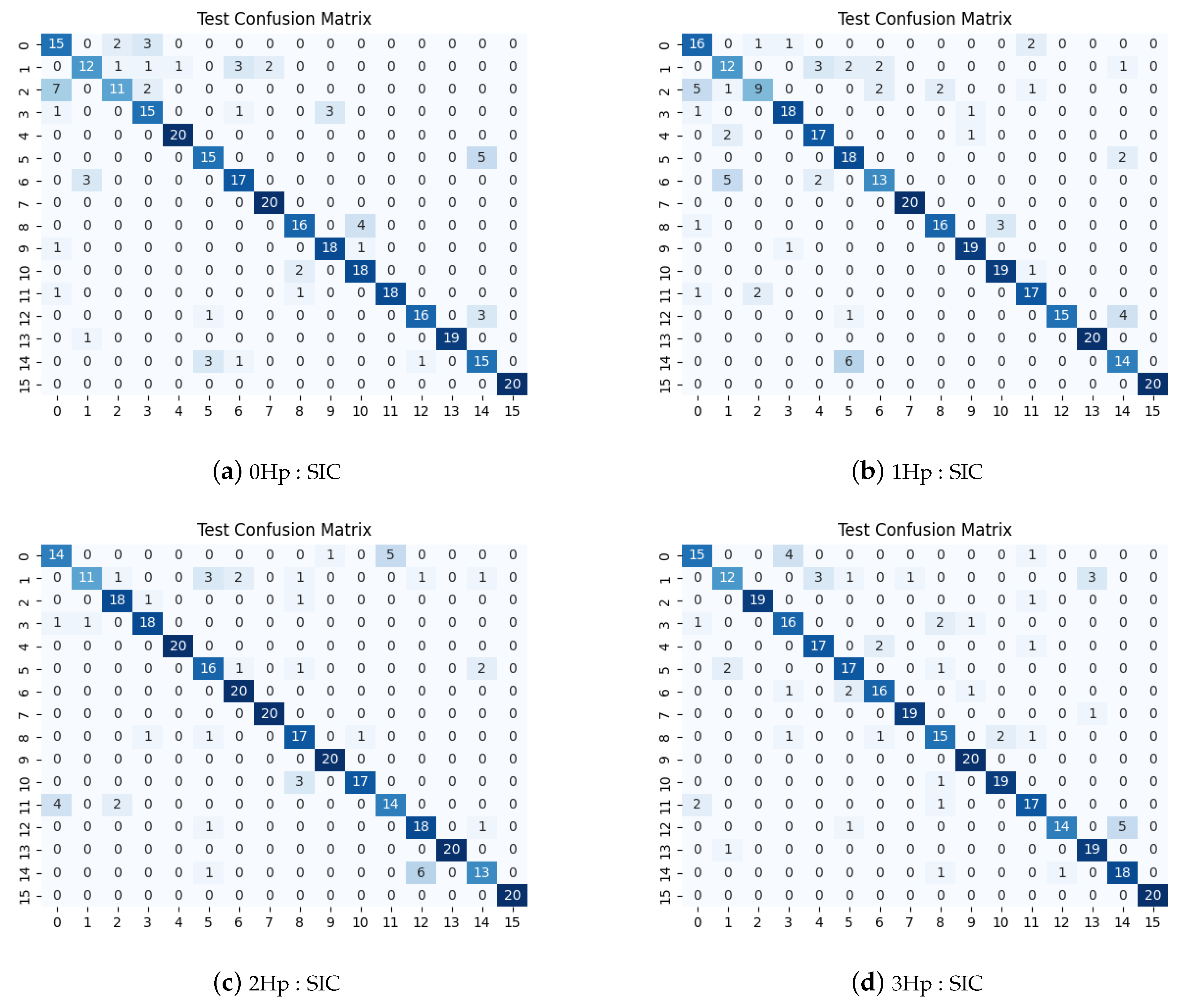
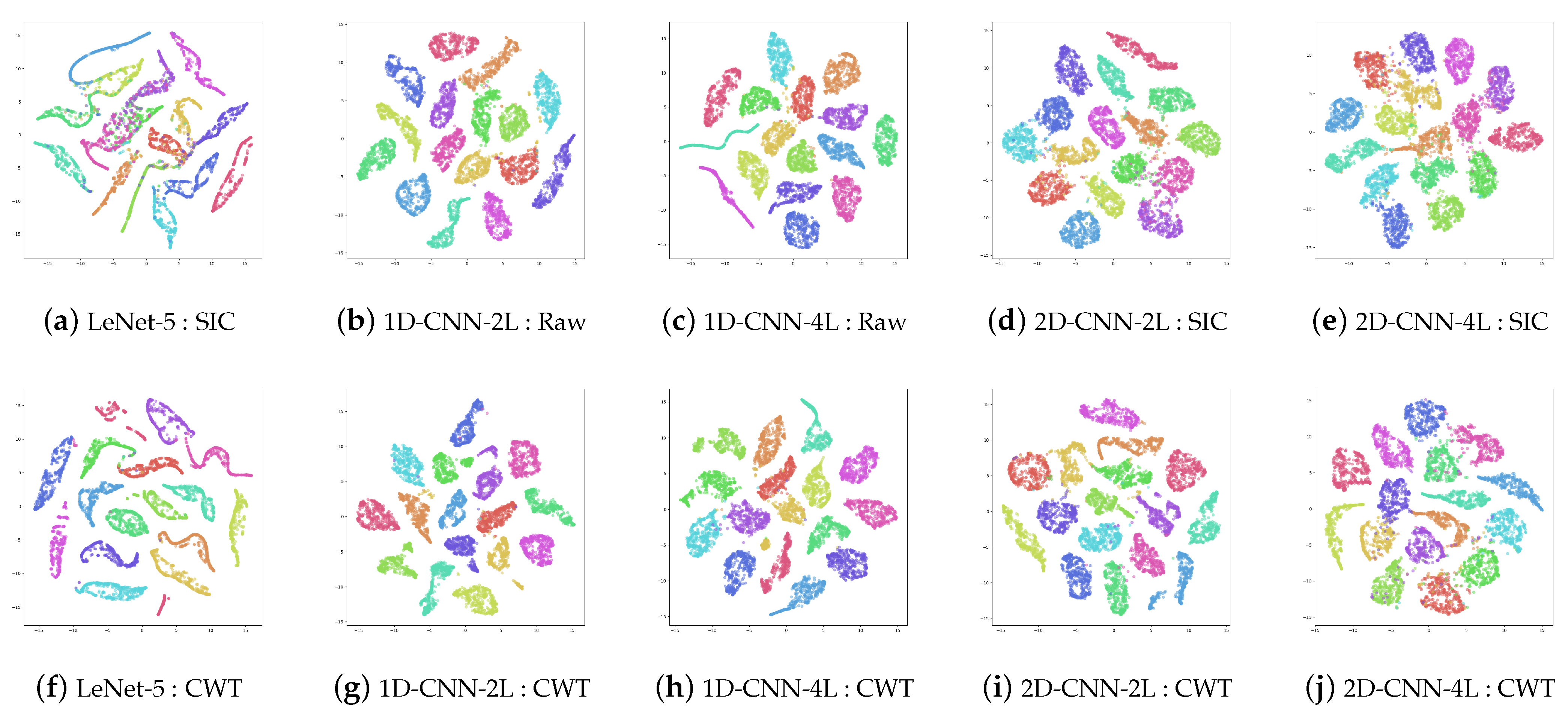
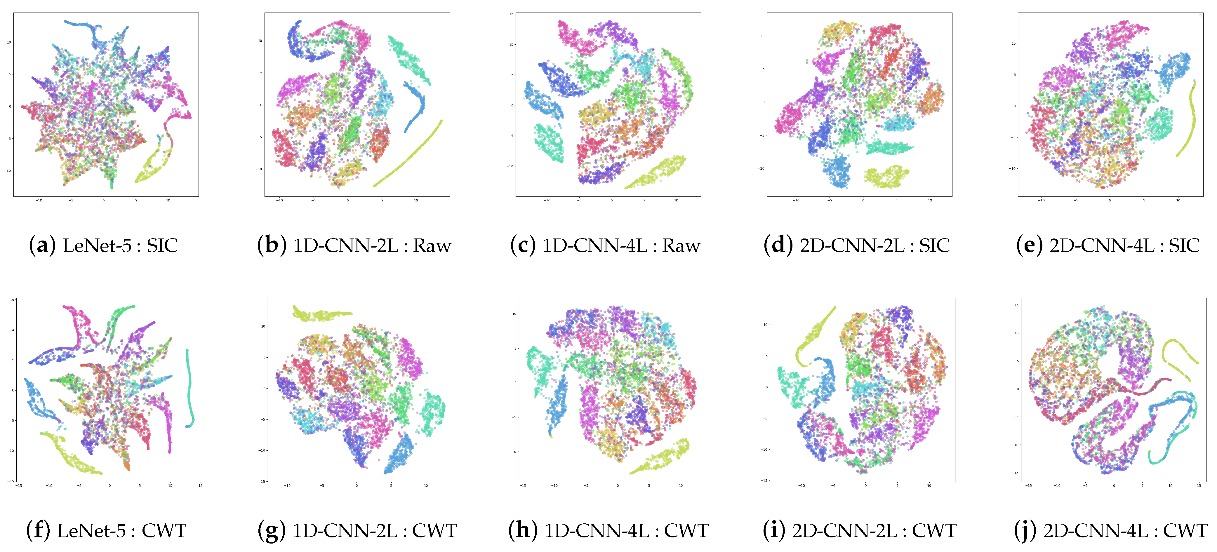
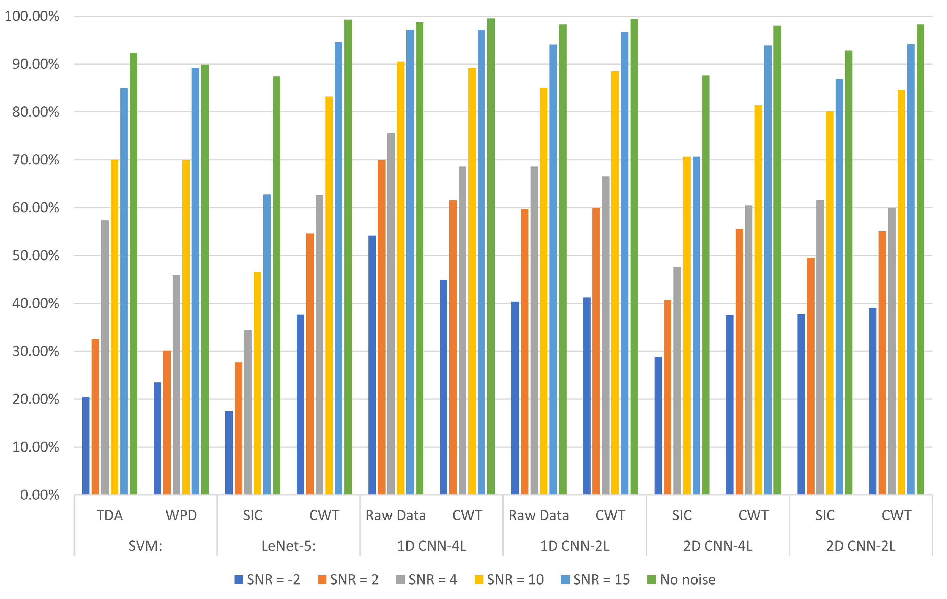
The field of fault diagnosis in electric machines has significantly attracted the interest of the research community. In this work, an evaluation study was conducted to find the most suitable signal preprocessing techniques and the most effective model for fault diagnosis of 16 conditions/classes, from a low-workload perspective using the well-known CWRU dataset. The data were preprocessed in various ways, including feature extraction in the time domain, wavelet packet decomposition, signal-to-image conversion and continuous wavelet transform. The processed data served as inputs to the classification models in order to evaluate the latter in terms of accuracy, noise resiliency and complexity. The learning models perform better when the noise is in a smaller fraction of the overall signal, as expected.

Table 16. Number of trainable parameters and training times for each learning model.

Models	Trainable Parameters	Training Time (s)
LeNet-5	62,216	55.89
2D CNN-2L	131,662	55.22
2D CNN-4L	115,918	37.95
1D CNN-2L	837,326	37.44
1D-CNN-4L	76,910	15.87

reports the number of trainable parameters and the training time for each neural network implementation. Generally, the 1D CNN has lower computational complexity and workload compared with the 2D operations needed for 2D CNN. This is also translated into faster training times for 1D CNN models. It is worth mentioning that, in the no-noise scenario, CWT is the best preprocessing method for all neural network implementations both handling the dataset with individual loading conditions (see Table 9, Table 10 and Table 11) and in the merged dataset (Table 12). Also, for the machine learning candidate (SVM), the best preprocessing technique is TDA compared with WPD. In the noisy environment scenario, TDA is again preferred over WPD for the SVM model (Table 13) and CWT leads to better classification accuracy for LeNet-5 and the other 2D CNN models (Table 13 and Table 14). In 1D CNN-4L, the best performing preprocessing method is the raw vibration signals (Table 15). However, 1D CNN-2L using CWT performs better than 1D CNN fed with raw vibration signals (Table 15), showing that, as the number of layers increases in 1D CNNs, raw signals are exploited more efficiently to classify bearing faults under heavy noise. Similar behavior is observed when all loading conditions are merged in a unified dataset as illustrated in Figure 11 from an oversight perspective.

Finally, in a “lessons learned” context we provide accumulated usual practices in the sense of preferred preprocessing methods and training models under different load and noise conditions:

• No-noise under individual load conditions:

  -

  Preprocessing method: For machine learning candidates, TDA is preferred over WPD. Apart from the better produced performance, TDA typically involves straightforward computations directly in the time domain which is often simpler to implement and computationally less intensive compared to frequency domain methods like Fourier transform. In the deep learning context CWT appears to be a strong approach as it consistently produced high accuracy results across different neural network architectures, including LeNet-5, 1D CNN-2L, 1D CNN-4L, 2D CNN-2L and 2D CNN-4L.

  -

  Training model: It appears that the 1D CNN model with four layers consistently performed very well across the different load conditions. This model is also relatively easier to implement compared to deep 2D convolutional architectures like LeNet-5 and 2D CNNs, making it an attractive choice in terms of both performance and simplicity.

• No-noise with all load conditions considered in a merged dataset:

  -

  Preprocessing method: In this case, TDA is preferred over WPD again, while, in the deep learning context, CWT appears to be again the most dominant approach in all training model cases. It should be noted that, with low deviation from the best performed approach, raw signals can be used in 1D implementations in the case that the lowest computational burden is needed from the signal processing perspective.

  -

  Training model: The most dominant model is 1D CNN-4L, while 1D CNN-2L and both 2D CNNs can also be used. However, the 1D CNN models seem to be more effective at capturing the relevant features of rolling bearing fault data compared with 2D CNNs. Also, 1D CNN architectures are generally simpler than 2D CNN architectures, both in terms of the model architecture and the number of parameters.

• Noisy environment under individual load conditions:

  -

  Preprocessing method: For machine learning candidates, WPD seems to perform slightly better under weak noise conditions only; thus, TDA is preferable in general in this case. For deep learning cases, CWT is clearly the most suitable for all cases with raw signals producing noise resilient forms in the 1D-CNN models.

  -

  Training model: It appears that the 1D CNN model with two layers performs better than 1D CNN-4L for weak noise conditions, but the latter is more resilient to medium and strong noise environments. In the 2D CNN implementations the one with two layers performs consistently better than the one which includes four layers. However, 1D CNN is preferred over 2D CNN in terms of performance and complexity.

• Noisy environment with all load conditions considered in a merged dataset:

  -

  Preprocessing method: In this case, WPD performs slightly better than TDA under strong noise but produces a degraded performance with respect to TDA in all other cases. In deep learning models, CWT provides a reliable preprocessing approach in all cases. However, the most resilient case is to include raw signals in deeper architectures of 1D CNN.

  -

  Training model: From the 2D CNN family, as the number of layers increases a less accurate performance is observed. In general, 1D CNN models seem to be well-suited to processing such data because they are designed to capture patterns along a single dimension, making them a natural choice for time series analysis. Deeper 1D CNN seems to work better with raw data in this generalized scenario under all noisy conditions. Also, this model provides the best choice from the computational burden perspective.

6. Conclusions

Different machine learning and deep learning models were evaluated utilizing different preprocessing methods. A low-cost (in terms of computational burden) orientation of the study was selected and, thus, evaluations were made on the 12 kHz of CWRU dataset considering all the trainable parameters. To align with possible real-time implementations, considering real-world noisy industrial environments, the performances of all adopted learning approaches from the preprocessing perspective under more feasible computational workloads were examined. Specifically, SVM, Lenet-5, 1D-CNN, and 2D-CNN from the feature extraction perspective, i.e., TDA, WPD, CWT and SIC, were evaluated, utilizing raw vibration signals acquired under varying load conditions of a 2 Hp induction motor with a sampling frequency of 12 kHz. Several findings were reported analytically and discussed.

References

1. Khan, M.A.; Asad, B.; Kudelina, K.; Vaimann, T.; Kallaste, A. The Bearing Faults Detection Methods for Electrical Machines—The State of the Art. Energies 2022, 16, 296. [Google Scholar] [CrossRef]
2. Jalan, A.K.; Mohanty, A. Model based fault diagnosis of a rotor–bearing system for misalignment and unbalance under steady-state condition. J. Sound Vib. 2009, 327, 604–622. [Google Scholar] [CrossRef]
3. Li, C.; Sanchez, V.; Zurita, G.; Lozada, M.C.; Cabrera, D. Rolling element bearing defect detection using the generalized synchrosqueezing transform guided by time–frequency ridge enhancement. ISA Trans. 2016, 60, 274–284. [Google Scholar] [CrossRef] [PubMed]
4. Cerrada, M.; Sánchez, R.V.; Li, C.; Pacheco, F.; Cabrera, D.; de Oliveira, J.V.; Vásquez, R.E. A review on data-driven fault severity assessment in rolling bearings. Mech. Syst. Signal Process. 2018, 99, 169–196. [Google Scholar] [CrossRef]
5. Wu, G.; Yan, T.; Yang, G.; Chai, H.; Cao, C. A Review on Rolling Bearing Fault Signal Detection Methods Based on Different Sensors. Sensors 2022, 22, 8330. [Google Scholar] [CrossRef]
6. Smith, W.A.; Randall, R.B. Rolling element bearing diagnostics using the Case Western Reserve University data: A benchmark study. Mech. Syst. Signal Process. 2015, 64, 100–131. [Google Scholar] [CrossRef]
7. Lee, J.; Qiu, H.; Yu, G.; Lin, J. Bearing Data Set, Nasa Ames Prognostics Data Repository; Rexnord Technical Services, IMS, University of Cincinnati: Cincinnati, OH, USA, 2007. [Google Scholar]
8. Lessmeier, C.; Kimotho, J.K.; Zimmer, D.; Sextro, W. Condition monitoring of bearing damage in electromechanical drive systems by using motor current signals of electric motors: A benchmark data set for data-driven classification. In Proceedings of the PHM Society European Conference, Bilbao, Spain, 5–8 July 2016; Volume 3. [Google Scholar]
9. Nectoux, P.; Gouriveau, R.; Medjaher, K.; Ramasso, E.; Chebel-Morello, B.; Zerhouni, N.; Varnier, C. PRONOSTIA: An experimental platform for bearings accelerated degradation tests. In Proceedings of the IEEE International Conference on Prognostics and Health Management, PHM’12, IEEE Catalog Number: CPF12PHM-CDR, Denver, CO, USA, 18–21 June 2012; pp. 1–8. [Google Scholar]
10. Nikula, R.P.; Karioja, K.; Pylvänäinen, M.; Leiviskä, K. Automation of low-speed bearing fault diagnosis based on autocorrelation of time domain features. Mech. Syst. Signal Process. 2020, 138, 106572. [Google Scholar] [CrossRef]
11. Liao, Y.; Sun, P.; Wang, B.; Qu, L. Extraction of repetitive transients with frequency domain multipoint kurtosis for bearing fault diagnosis. Meas. Sci. Technol. 2018, 29, 055012. [Google Scholar] [CrossRef]
12. Pandhare, V.; Singh, J.; Lee, J. Convolutional neural network based rolling-element bearing fault diagnosis for naturally occurring and progressing defects using time-frequency domain features. In Proceedings of the 2019 Prognostics and System Health Management Conference (PHM-Paris), Paris, France, 2–5 May 2019; IEEE: New York, NY, USA, 2019; pp. 320–326. [Google Scholar]
13. Nayana, B.; Geethanjali, P. Analysis of statistical time-domain features effectiveness in identification of bearing faults from vibration signal. IEEE Sens. J. 2017, 17, 5618–5625. [Google Scholar] [CrossRef]
14. Pandarakone, S.E.; Masuko, M.; Mizuno, Y.; Nakamura, H. Deep neural network based bearing fault diagnosis of induction motor using fast Fourier transform analysis. In Proceedings of the 2018 IEEE Energy Conversion Congress and Exposition (ECCE), Portland, OR, USA, 23–27 September 2018; IEEE: New York, NY, USA, 2018; pp. 3214–3221. [Google Scholar]
15. Esakimuthu Pandarakone, S.; Mizuno, Y.; Nakamura, H. A comparative study between machine learning algorithm and artificial intelligence neural network in detecting minor bearing fault of induction motors. Energies 2019, 12, 2105. [Google Scholar] [CrossRef]
16. Cocconcelli, M.; Zimroz, R.; Rubini, R.; Bartelmus, W. STFT based approach for ball bearing fault detection in a varying speed motor. In Proceedings of the Second International Conference “Condition Monitoring of Machinery in Non-Stationnary Operations” CMMNO’2012; Springer: Berlin/Heidelberg, Germany, 2012; pp. 41–50. [Google Scholar]
17. Kankar, P.K.; Sharma, S.C.; Harsha, S.P. Fault diagnosis of ball bearings using continuous wavelet transform. Appl. Soft Comput. 2011, 11, 2300–2312. [Google Scholar] [CrossRef]
18. Du, J.; Li, X.; Gao, Y.; Gao, L. Integrated Gradient-Based Continuous Wavelet Transform for Bearing Fault Diagnosis. Sensors 2022, 22, 8760. [Google Scholar] [CrossRef]
19. Ocak, H.; Loparo, K.A.; Discenzo, F.M. Online tracking of bearing wear using wavelet packet decomposition and probabilistic modeling: A method for bearing prognostics. J. Sound Vib. 2007, 302, 951–961. [Google Scholar] [CrossRef]
20. Li, Y.; Xu, M.; Huang, W.; Zuo, M.J.; Liu, L. An improved EMD method for fault diagnosis of rolling bearing. In Proceedings of the 2016 Prognostics and System Health Management Conference (PHM-Chengdu), Chengdu, China, 19–21 October 2016; IEEE: New York, NY, USA, 2016; pp. 1–5. [Google Scholar]
21. Li, H.; Liu, T.; Wu, X.; Chen, Q. An optimized VMD method and its applications in bearing fault diagnosis. Measurement 2020, 166, 108185. [Google Scholar] [CrossRef]
22. El Idrissi, A.; Derouich, A.; Mahfoud, S.; El Ouanjli, N.; Chantoufi, A.; Al-Sumaiti, A.; Mossa, M.A. Bearing Fault Diagnosis for an Induction Motor Controlled by an Artificial Neural Network—Direct Torque Control Using the Hilbert Transform. Mathematics 2022, 10, 4258. [Google Scholar] [CrossRef]
23. Huang, W.; Zhang, G.; Jiao, S.; Wang, J. Bearing Fault Diagnosis Based on Stochastic Resonance and Improved Whale Optimization Algorithm. Electronics 2022, 11, 2185. [Google Scholar] [CrossRef]
24. Yan, X.; Jia, M. A novel optimized SVM classification algorithm with multi-domain feature and its application to fault diagnosis of rolling bearing. Neurocomputing 2018, 313, 47–64. [Google Scholar] [CrossRef]
25. Pandya, D.; Upadhyay, S.H.; Harsha, S.P. Fault diagnosis of rolling element bearing with intrinsic mode function of acoustic emission data using APF-KNN. Expert Syst. Appl. 2013, 40, 4137–4145. [Google Scholar] [CrossRef]
26. You, K.; Qiu, G.; Gu, Y. Rolling Bearing Fault Diagnosis Using Hybrid Neural Network with Principal Component Analysis. Sensors 2022, 22, 8906. [Google Scholar] [CrossRef]
27. Li, H.; Liu, T.; Wu, X.; Chen, Q. A bearing fault diagnosis method based on enhanced singular value decomposition. IEEE Trans. Ind. Inform. 2020, 17, 3220–3230. [Google Scholar] [CrossRef]
28. Karatzinis, G.; Boutalis, Y.S.; Karnavas, Y.L. Motor fault detection and diagnosis using fuzzy cognitive networks with functional weights. In Proceedings of the 2018 26th Mediterranean Conference on Control and Automation (MED), Zadar, Croatia, 19–22 June 2018; IEEE: New York, NY, USA, 2018; pp. 709–714. [Google Scholar]
29. Li, Y.; Mu, L.; Gao, P. Particle swarm optimization fractional slope entropy: A new time series complexity indicator for bearing fault diagnosis. Fractal Fract. 2022, 6, 345. [Google Scholar] [CrossRef]
30. Liu, Y.; Chai, Y.; Liu, B.; Wang, Y. Bearing fault diagnosis based on energy spectrum statistics and modified mayfly optimization algorithm. Sensors 2021, 21, 2245. [Google Scholar] [CrossRef]
31. Zhou, J.; Xiao, M.; Niu, Y.; Ji, G. Rolling Bearing Fault Diagnosis Based on WGWOA-VMD-SVM. Sensors 2022, 22, 6281. [Google Scholar] [CrossRef]
32. Zhao, B.; Zhang, X.; Li, H.; Yang, Z. Intelligent fault diagnosis of rolling bearings based on normalized CNN considering data imbalance and variable working conditions. Knowl.-Based Syst. 2020, 199, 105971. [Google Scholar] [CrossRef]
33. Liu, X.; Sun, W.; Li, H.; Hussain, Z.; Liu, A. The Method of Rolling Bearing Fault Diagnosis Based on Multi-Domain Supervised Learning of Convolution Neural Network. Energies 2022, 15, 4614. [Google Scholar] [CrossRef]
34. Meng, Z.; Zhan, X.; Li, J.; Pan, Z. An enhancement denoising autoencoder for rolling bearing fault diagnosis. Measurement 2018, 130, 448–454. [Google Scholar] [CrossRef]
35. Lu, C.; Wang, Z.Y.; Qin, W.L.; Ma, J. Fault diagnosis of rotary machinery components using a stacked denoising autoencoder-based health state identification. Signal Process. 2017, 130, 377–388. [Google Scholar] [CrossRef]
36. Che, C.; Wang, H.; Ni, X.; Fu, Q. Domain adaptive deep belief network for rolling bearing fault diagnosis. Comput. Ind. Eng. 2020, 143, 106427. [Google Scholar] [CrossRef]
37. Jiang, H.; Li, X.; Shao, H.; Zhao, K. Intelligent fault diagnosis of rolling bearings using an improved deep recurrent neural network. Meas. Sci. Technol. 2018, 29, 065107. [Google Scholar] [CrossRef]
38. An, Y.; Zhang, K.; Liu, Q.; Chai, Y.; Huang, X. Rolling bearing fault diagnosis method base on periodic sparse attention and LSTM. IEEE Sensors J. 2022, 22, 12044–12053. [Google Scholar] [CrossRef]
39. Pham, M.T.; Kim, J.M.; Kim, C.H. Rolling bearing fault diagnosis based on improved GAN and 2-D representation of acoustic emission signals. IEEE Access 2022, 10, 78056–78069. [Google Scholar] [CrossRef]
40. Abdelkader, R.; Kaddour, A.; Derouiche, Z. Enhancement of rolling bearing fault diagnosis based on improvement of empirical mode decomposition denoising method. Int. J. Adv. Manuf. Technol. 2018, 97, 3099–3117. [Google Scholar] [CrossRef]
41. Bao, G.; Chang, Y.; He, T. An EMD threshold-based de-noising method for roller bearing fault vibration signal analysis. J. Comput. Inf. Syst. 2014, 10, 7645–7652. [Google Scholar]
42. Shenfield, A.; Howarth, M. A novel deep learning model for the detection and identification of rolling element-bearing faults. Sensors 2020, 20, 5112. [Google Scholar] [CrossRef]
43. Wan, L.; Chen, Y.; Li, H.; Li, C. Rolling-element bearing fault diagnosis using improved LeNet-5 network. Sensors 2020, 20, 1693. [Google Scholar] [CrossRef]
44. Jin, G.; Zhu, T.; Akram, M.W.; Jin, Y.; Zhu, C. An adaptive anti-noise neural network for bearing fault diagnosis under noise and varying load conditions. IEEE Access 2020, 8, 74793–74807. [Google Scholar] [CrossRef]
45. Qiao, M.; Yan, S.; Tang, X.; Xu, C. Deep convolutional and LSTM recurrent neural networks for rolling bearing fault diagnosis under strong noises and variable loads. IEEE Access 2020, 8, 66257–66269. [Google Scholar] [CrossRef]
46. Akbar, S.; Vaimann, T.; Asad, B.; Kallaste, A.; Sardar, M.U.; Kudelina, K. State-of-the-Art Techniques for Fault Diagnosis in Electrical Machines: Advancements and Future Directions. Energies 2023, 16, 6345. [Google Scholar] [CrossRef]
47. Alexakos, C.T.; Karnavas, Y.L.; Drakaki, M.; Tziafettas, I.A. A Combined Short Time Fourier Transform and Image Classification Transformer Model for Rolling Element Bearings Fault Diagnosis in Electric Motors. Mach. Learn. Knowl. Extr. 2021, 3, 228–242. [Google Scholar] [CrossRef]
48. Nieves Avendano, D.; Vandermoortele, N.; Soete, C.; Moens, P.; Ompusunggu, A.P.; Deschrijver, D.; Van Hoecke, S. A semi-supervised approach with monotonic constraints for improved remaining useful life estimation. Sensors 2022, 22, 1590. [Google Scholar] [CrossRef]
49. Yan, M.; Wang, X.; Wang, B.; Chang, M.; Muhammad, I. Bearing remaining useful life prediction using support vector machine and hybrid degradation tracking model. ISA Trans. 2020, 98, 471–482. [Google Scholar] [CrossRef]
50. Boudiaf, A.; Moussaoui, A.; Dahane, A.; Atoui, I. A comparative study of various methods of bearing faults diagnosis using the case Western Reserve University data. J. Fail. Anal. Prev. 2016, 16, 271–284. [Google Scholar] [CrossRef]
51. Rai, A.; Upadhyay, S.H. A review on signal processing techniques utilized in the fault diagnosis of rolling element bearings. Tribol. Int. 2016, 96, 289–306. [Google Scholar] [CrossRef]
52. Mao, W.; Wang, L.; Feng, N. A new fault diagnosis method of bearings based on structural feature selection. Electronics 2019, 8, 1406. [Google Scholar] [CrossRef]
53. Tang, X.; Wang, J.; Lu, J.; Liu, G.; Chen, J. Improving bearing fault diagnosis using maximum information coefficient based feature selection. Appl. Sci. 2018, 8, 2143. [Google Scholar] [CrossRef]
54. Rauber, T.W.; de Assis Boldt, F.; Varejao, F.M. Heterogeneous feature models and feature selection applied to bearing fault diagnosis. IEEE Trans. Ind. Electron. 2014, 62, 637–646. [Google Scholar] [CrossRef]
55. Samanta, B.; Al-Balushi, K.; Al-Araimi, S. Artificial neural networks and support vector machines with genetic algorithm for bearing fault detection. Eng. Appl. Artif. Intell. 2003, 16, 657–665. [Google Scholar] [CrossRef]
56. Konar, P.; Chattopadhyay, P. Bearing fault detection of induction motor using wavelet and Support Vector Machines (SVMs). Appl. Soft Comput. 2011, 11, 4203–4211. [Google Scholar] [CrossRef]
57. Tian, J.; Morillo, C.; Azarian, M.H.; Pecht, M. Motor bearing fault detection using spectral kurtosis-based feature extraction coupled with K-nearest neighbor distance analysis. IEEE Trans. Ind. Electron. 2015, 63, 1793–1803. [Google Scholar] [CrossRef]
58. Guo, X.; Shen, C.; Chen, L. Deep fault recognizer: An integrated model to denoise and extract features for fault diagnosis in rotating machinery. Appl. Sci. 2016, 7, 41. [Google Scholar] [CrossRef]
59. Zhang, J.; Yi, S.; Liang, G.; Hongli, G.; Xin, H.; Hongliang, S. A new bearing fault diagnosis method based on modified convolutional neural networks. Chin. J. Aeronaut. 2020, 33, 439–447. [Google Scholar] [CrossRef]
60. Eren, L.; Ince, T.; Kiranyaz, S. A generic intelligent bearing fault diagnosis system using compact adaptive 1D CNN classifier. J. Signal Process. Syst. 2019, 91, 179–189. [Google Scholar] [CrossRef]
61. Zhao, H.; Yang, X.; Chen, B.; Chen, H.; Deng, W. Bearing fault diagnosis using transfer learning and optimized deep belief network. Meas. Sci. Technol. 2022, 33, 065009. [Google Scholar] [CrossRef]
62. Yang, Z.b.; Zhang, J.p.; Zhao, Z.b.; Zhai, Z.; Chen, X.f. Interpreting network knowledge with attention mechanism for bearing fault diagnosis. Appl. Soft Comput. 2020, 97, 106829. [Google Scholar] [CrossRef]
63. Zhang, X.; Zhao, B.; Lin, Y. Machine learning based bearing fault diagnosis using the case western reserve university data: A review. IEEE Access 2021, 9, 155598–155608. [Google Scholar] [CrossRef]
64. Zhang, S.; Zhang, S.; Wang, B.; Habetler, T.G. Deep learning algorithms for bearing fault diagnostics—A comprehensive review. IEEE Access 2020, 8, 29857–29881. [Google Scholar] [CrossRef]
65. Neupane, D.; Seok, J. Bearing fault detection and diagnosis using case western reserve university dataset with deep learning approaches: A review. IEEE Access 2020, 8, 93155–93178. [Google Scholar] [CrossRef]
66. Sun, H.; Cao, X.; Wang, C.; Gao, S. An interpretable anti-noise network for rolling bearing fault diagnosis based on FSWT. Measurement 2022, 190, 110698. [Google Scholar] [CrossRef]
67. Peng, D.; Wang, H.; Liu, Z.; Zhang, W.; Zuo, M.J.; Chen, J. Multibranch and multiscale CNN for fault diagnosis of wheelset bearings under strong noise and variable load condition. IEEE Trans. Ind. Inform. 2020, 16, 4949–4960. [Google Scholar] [CrossRef]
68. Chen, X.; Zhang, B.; Gao, D. Bearing fault diagnosis base on multi-scale CNN and LSTM model. J. Intell. Manuf. 2021, 32, 971–987. [Google Scholar] [CrossRef]
69. Zhu, H.; He, Z.; Wei, J.; Wang, J.; Zhou, H. Bearing Fault Feature Extraction and Fault Diagnosis Method Based on Feature Fusion. Sensors 2021, 21, 2524. [Google Scholar] [CrossRef] [PubMed]
70. Zhao, L.Y.; Wang, L.; Yan, R.Q. Rolling bearing fault diagnosis based on wavelet packet decomposition and multi-scale permutation entropy. Entropy 2015, 17, 6447–6461. [Google Scholar] [CrossRef]
71. Xia, Z.; Xia, S.; Wan, L.; Cai, S. Spectral regression based fault feature extraction for bearing accelerometer sensor signals. Sensors 2012, 12, 13694–13719. [Google Scholar] [CrossRef] [PubMed]
72. Büssow, R. An algorithm for the continuous Morlet wavelet transform. Mech. Syst. Signal Process. 2007, 21, 2970–2979. [Google Scholar] [CrossRef]
73. Wen, L.; Li, X.; Gao, L.; Zhang, Y. A new convolutional neural network-based data-driven fault diagnosis method. IEEE Trans. Ind. Electron. 2017, 65, 5990–5998. [Google Scholar] [CrossRef]
Figure 1. Rolling bearing geometry.
Machines 11 01029 g001
Figure 2. Visual representation of the rolling bearing fault detection process from the CNN perspective using different feature extraction methods.
Machines 11 01029 g002
Figure 3. CWRU testbed.
Machines 11 01029 g003
Figure 4. Indicative samples of raw vibration signals.
Machines 11 01029 g004
Figure 5. Schematic diagram of a WPD tree with three levels.
Machines 11 01029 g005
Figure 6. Indicative examples of continuous wavelet transform.
Machines 11 01029 g006
Figure 7. Indicative examples of signal-to-image conversion.
Machines 11 01029 g007
Figure 8. Confusion matrices of 2D CNN-2L model for SIC data.
Machines 11 01029 g008
Figure 9. Feature representation for all learning models in their last dense layer under normal conditions (no-noise).
Machines 11 01029 g009
Figure 10. Feature representation for all learning models in their last dense layer in noisy environments (SNR = −2).
Machines 11 01029 g010
Figure 11. Overall performance for all models with respect to the different SNR values for the merged dataset case (all loading conditions).
Machines 11 01029 g011