1. Introduction
Reliability and efficiency of industrial equipment are essential aspects playing key roles to raise as much as possible the productivity, avoiding unexpected stoppages and their related maintenance-repairing costs [
1,
2]. In this context, the induction motor (IM) is still considered one of the most important machines in industry, because it allows for transmitting the mechanical motion, rotative or linear, in the existing industrial applications [
3,
4]. The versatility of this machine allows it to be implemented in several applications, commercial and industrial, such as conveyors, fans, blowers, compressors, shredders, pumps, cranes, lifts, refrigeration, and transportation, among others [
3]. Now, the main reasons for using IMs are their easy maintenance, high power efficiency, high reliability, low cost, wide applicability, good relation speed–torque output, manufacturing robustness, simple design, industrial environment resistance, and so on [
5,
6,
7]. In fact, IMs are widely used around the world and many reported investigations indicate that this engine represents above 80% of the rotative machines in industry [
8]. In addition, these motors consume, from the total of the energy required and used by the industries, levels that reach between 40% and 80% [
2,
6,
9,
10]. Therefore, from all this information, it is clear why the IMs are still a topic of interest, since any slight or significative improvement on its operation, design, diagnostic, or maintenance process will impact positively in several desirable requirements of companies like the economical, the technological, and the environmental.
The IMs are ensembles of important parts like the stator, the rotor, the windings, the rotor shaft, the fan, and the bearings of the shaft and the fan [
4,
11]. Additionally, several works have found that the previously mentioned components are associated with specific machine faults [
12,
13]; to this respect, the most common faults correspond to bearing damage in the range of 40% to 51%, followed by stator problems between 16% and 40%; the next are rotor damages with 5% to 10%, and other associated problems appear in a range of 12% to 28% [
11,
12,
14]. Therefore, it is noticed that second major problems found in IMs are an electric type associated with the stator component, particularly, the stator winding faults (SWFs) such as short circuits and damage occurring turn-to-turn, coil-to-coil, phase-to-phase, or phase-to-ground [
11]. In general, the winding faults encompass about two-thirds of the failures occurring in the stator for high-power motors. However, the well-known inter-turn short-circuit (ITSC) faults are of interest in this work, because they have been reported as the most common, accounting for between 30% and 40% of the winding faults [
15]. The ITSC faults are problems in the insulation along the winding for the same phase due to the industrial environment and the motor operating conditions [
16]. For example, the excessive current values flowing through the windings above their limits accelerate the insulation degradation; but also, the fast switching of inverters based on pulse-width modulation driving the motor affects it similarly [
17,
18]. The ITSC faults bring as a consequence malfunctioning of the motor associated with overheating, slight vibration, asymmetric behavior noticed as audible noise, magnetic saturation, and poor performance [
18,
19]. In conclusion, the monitoring and diagnosing of industrial equipment allow for developing adequate maintenance planning to avoid catastrophic damage through effective predictive actions.
In relation to the diagnostics of ITSC faults, there exist several classic methodologies based on stator current, stator voltage, mechanical output, parameter estimation, and even magnetic flux [
17]. Many works were initially model-based, for example, the physical parameters of a motor (resistances and inductances) were analyzed on a mathematical model for a five-phase permanent-magnet synchronous motor (PMSM) in [
20]; posteriorly, a trust region algorithm uses an objective function for indicating the ratio of the ITSC. In another work [
21], the modelling of a stator end winding of a six-pole synchronous generator is developed based on a qualitative theoretical analysis, a finite element analysis (FEA), and experimental validation. Also, that work studies the effects of the ITSC positions on the end winding electromagnetic forces according to the static air-gap eccentricity. In another case, the effects of ITSC in the field winding, causing rotor vibrations, for turbo generators are investigated in [
22]. In that work, the unbalanced magnetic pull (UMP) model was obtained through a theoretical analysis of the magnetic flux density (MFD) variation, next was an FEA determining UMP data, and at last, rotor vibrations were tested on a two-pole 5 kVA generator prototype. Regarding the methodologies based on the classic measurements of stator currents, vibrations, and magnetic flux, several works have been proposed; for instance, in [
23], an approach based on the time-frequency analysis and the wavelet packet transform (WPT) detected inter-turn faults in the stator winding of a PMSM. There, the stator current and vibration signals were used in the approach under a LabVIEW environment. Another example is the statistical methodology presented in [
24] that uses the Pearson coefficient between two voltage signals measured with external flux sensors located symmetrically around the induction motor under different load conditions. Furthermore, in [
25], a harmonic analysis for detecting ITSC is applied for different electrical signatures of a stator current, external magnetic flux, and electromechanical torque, under different load levels of squirrel cage IMs. There, the FEA is used to simulate the IM behavior for comparing the current-saturation-related harmonics, the magnetomotive-force-related harmonics, and the stray-flux harmonics at certain frequencies. From the discussion of the previous works, the classic approaches were helpful when the physical systems were not available (model-based) and software tools make it possible to simulate systems’ behavior, but in a modeling process, many assumptions need to be carried out. Meanwhile, the methodologies based on a frequency analysis strongly depend on the fault-related frequencies, which is a disadvantage when other fault frequencies appear. Finally, the statistical analysis is useful in detecting short circuits; then, it would be worthwhile to explore the use of multiple indicators when the faults are combined or under different operating conditions.
Recently, new methodologies have been developed under novel and powerful schemes that process high-dimensional data, for example, data-driven approaches like in [
26], where an online detection of ITSC was performed on IMs. In such work, several signals are measured for extracting multiple features, and later several classifiers like support vector machines (SVMs), naïve bayes (NB), neural networks (NNs), and an extreme learning machine (ELM) are applied for detecting the faults. In another instance, the data driving of digital twin models is applied for diagnosing ITSC in a PMSM [
27]. For that application, the digital twin is specified in the healthy state through an auto-regressive model with exogenous inputs (NARX). Regarding the methodologies based in machine learning, the research in [
28] proposes a scheme for detecting ITSC faults in a PMSM by extracting features through SVM, and classifying them through convolutional neural networks (CNNs). Another example is the ITSC faults’ diagnostic based on a random forest (RF) model developed in [
29] for an electronic multiple unit (EMU) traction motor. To achieve that, a Goertzel algorithm computes current amplitude differences and phase angle differences of three fault conditions that are fed to the RF. Now, an example of a deep learning approach is the manuscript presented in [
30], where the ITSC diagnosis is addressed for PMSM by means of a conditional generative adversarial net (CGAN), to augment the number of the collected samples, and a sparse auto encoder (OSAE) for the classification. A last example is the work in [
31], where a tool for diagnosing stator winding faults is proposed by using NN to estimate the percentage of shorted turns on the IMs. Nevertheless, the model of the network is developed under a MATLAB environment under different load and fault conditions, and for different motor sizes. From the previously discussed works, for each stage (processing, feature extraction, pattern recognition/learning), there exist several techniques with their own advantages and disadvantages, so their adequate selection and combination will define the methodology success, and it can be seen as an area of opportunity for the early appearance of incipient ITSC faults.
This work proposes an approach that fuses empirical wavelet transform (EWT) and self-organizing maps (SOMs) to identify and characterize the time frequency behavior of an IM that works with different severities of an ITSC fault. The contributions of this work can be summarized as follows:
The design of an incipient fault detection technique that works during the IM transient start-up, allowing to obtain more reliable and accurate results since it has been reported that the steady-state analysis experiments create more troubles for the fault identification [
32,
33].
The development of a high-performance method that properly works even in noisy environments. This situation is allowed due to the use of EWT that works as a series of adaptive band-pass filters, allowing to separate the noise content in a high-frequency band that is not considered in the next stages.
The proposal of an optimal fault modeling and characterization method by means of a genetic algorithm (GA) and SOM. The GA allows for preserving only the relevant features while SOM individually models the behavior of every operating condition, resulting in a high fault detection and classification accuracy.
It is important to mention that the proposed methodology detects four different operating conditions (healthy condition and three different insipient ITSC severities). Additionally, the approach can be applied to the IM regardless of its operation frequency. To prove this, several tests were performed during the start-up transient but considering that the IM reaches four different final operating frequencies: 15 Hz, 30 Hz, 50 Hz, and 60 Hz. Results show that the proposed methodology can detect and classify the operating conditions with high accuracy, being robust and reliable. The paper is structured as follows:
Section 2 presents the description of materials and methods that were implemented to achieve the diagnosis of the ITSC faults. In
Section 3, the experimental setup and data acquisition system (DAS) used to perform the experimentation are described.
Section 4 shows the results obtained from the experimentation on the IM; they are accompanied with a discussion of the main insights found by applying the proposed methodology. Finally,
Section 5 presents the conclusions and perspectives that result from this work.
2. Materials and Methods
Induction motors (IMs) are commonly subjected to mechanical and electrical stresses due to their robustness; however, the unexpected occurrence of faults may cause inappropriate operating conditions that can lead to a catastrophic breakdown. In this regard, the most common problems that affect the operation of IMs are those associated with the rotor and/or the stator winding, i.e., failures generated with damaged bearings, unbalances, misalignments, broken bars, and short circuits. Certainly, short circuits are considered the most critical damage since they can occur in very short periods; hence, the stator inter-turn short circuit (ITSC) is a defect that is related to the insulation of the stator winding. Consequently, the stator current signatures of IMs are affected by an amplitude increase when operating under the effect of ITSC; additionally, the density of the air-gap flux is also affected by the occurrence of ITSC. Accordingly, the identification of ITSC in IMs can be performed by following classic strategies based on the motor current signature analysis (MCSA), specifically by locating those fault-related frequency components (
) into the stator current spectra, by following Equation (1):
where
is the supply frequency that is used to feed the IM,
depicts the per unit slip,
represents the number of pole pairs, and
and
are defined as integers (
and
). Although the assessments of ITSC can be carried out through MCSA following Equation (1), it should be highlighted that this approach is limited to be applied under the steady-state regime of the IM; this limitation is due to the stator current spectra that are estimated with the Fast Fourier Transform (FFT) technique. Moreover, the detection of ITSC through the FFT involves the measurement of current signatures during the steady-state regime for an extended period of time in order to obtain frequency spectra with a high resolution; nevertheless, long operations under the influence of ITSC can produce irreversible damage.
Therefore, the early detection of ITSC in IMs may guarantee their availability and can lead to the application of preventive maintenance actions; in this regard, this work proposes a diagnosis methodology for detecting the occurrence of ITSC in IMs during the start-up transient regime. Hence, the method includes the acquisition of the stator current signatures from an IM that operates under different severities of ITSC, as well as the processing of the acquired signals through the EWT to obtain a set of patterns that characterize the start-up transient regime of the IM. Then, each decomposition obtained with the EWT is subsequently characterized by estimating a set of 15 statistical features to generate a high-dimensional set of features. Additionally, the proposed method is supported with a structure based on several SOMs in conjunction with a genetic algorithm; the aim of this structure is to select and model the most representative patterns that better depict the transient behavior of each tested condition in the IM. Formerly, the different conditions are individually modelled with a specific SOM neuron grid and the LDA is used to compress the information provided with the whole SOM neuron grids into a 2
d projection and they are represented in all studied cases. Finally, the diagnosis and detection of different severities of ITSC are achieved with a neural-network-based (NN) classifier.
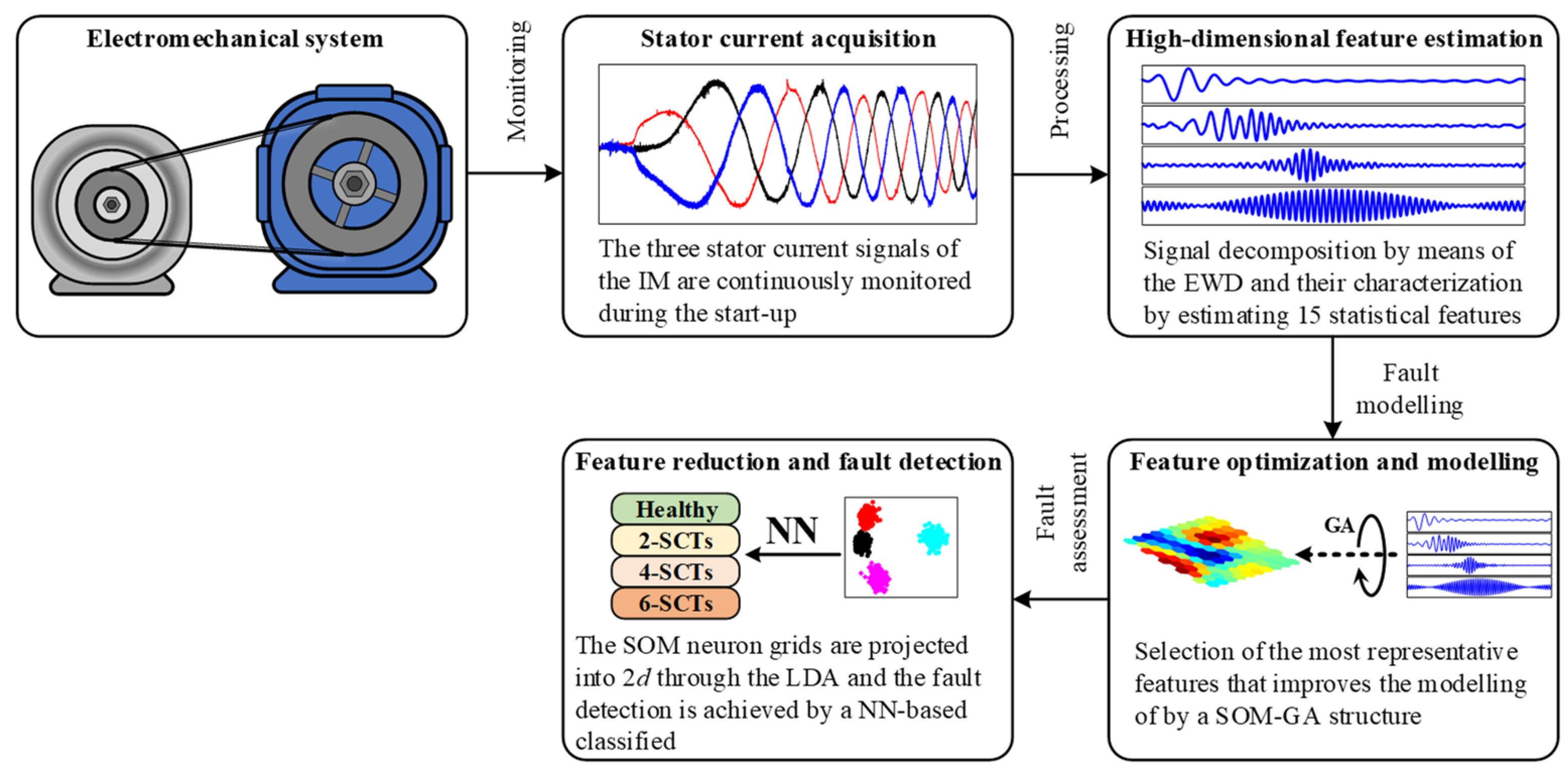
Figure 1 shows the flow chart of the proposed method for detecting the appearance of ITSC in IMs during a start-up transient regime.
2.1. Electromechanical System
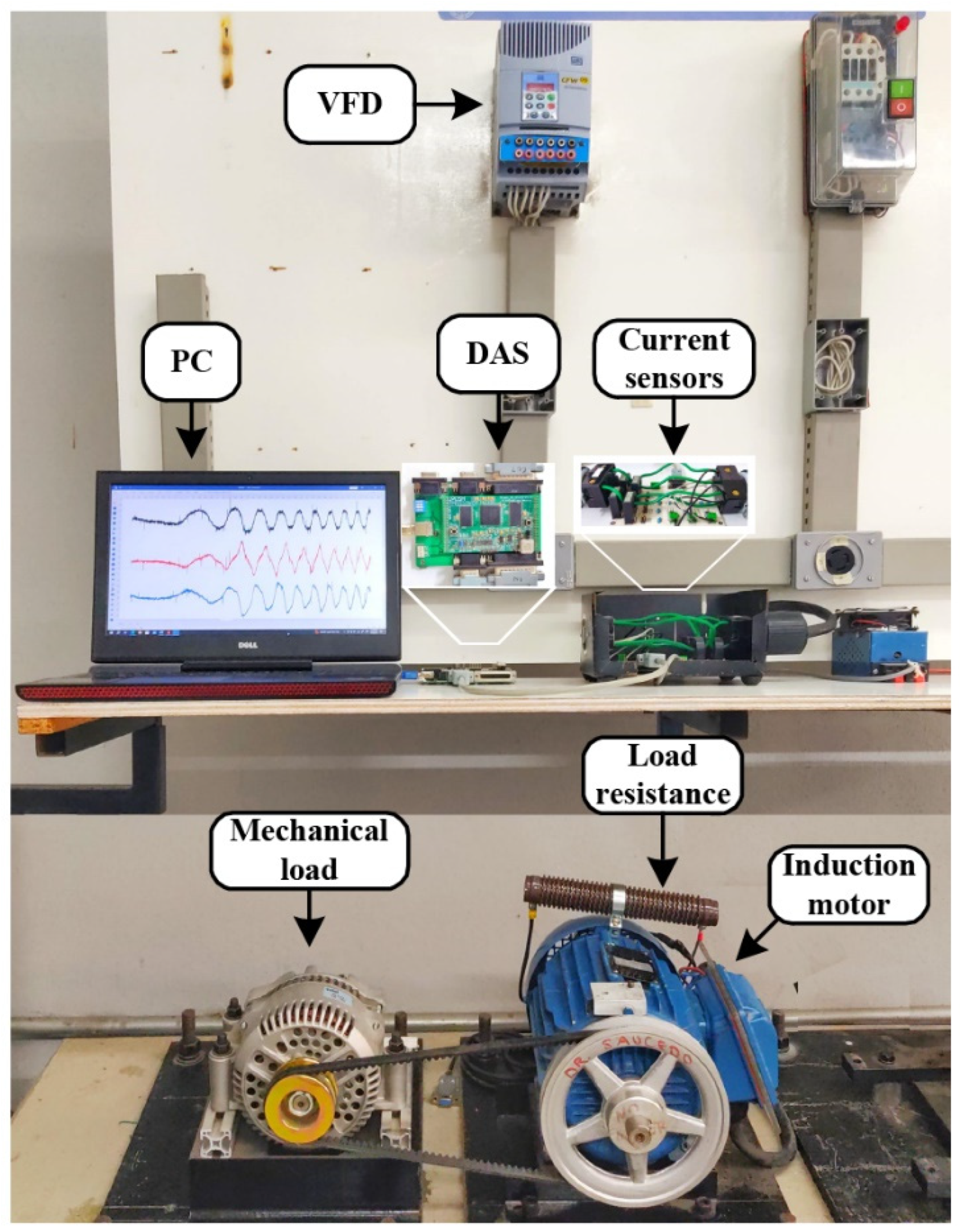
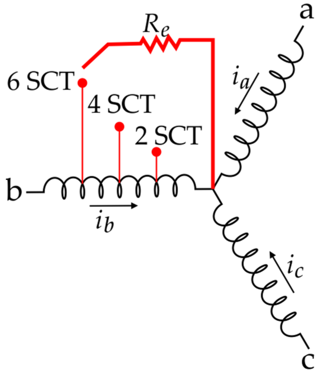
The electromechanical system is the system where different severities of SCTs are tested; specifically, the system is a pulley-belt-based system that is mainly composed of an IM that drives a conventional automotive alternator used as the mechanical load. Regarding the studied conditions, in the IM are individually tested four different conditions, which are the healthy condition (HLT) and three fault severities that consider 2, 4, and 6 SCTs; moreover, each considered condition is tested under different operating frequencies (15 Hz, 30 Hz, 50 Hz, and 60 Hz) to produce different rotating frequencies in the output shaft of the IM. In the electromechanical system, a set of three hall-effect current sensors are installed to measure the stator current consumption with the aim of monitoring the behavior produced with the influence of the aforementioned conditions in the start-up transient regime of the IM.
2.2. Stator Current Acquisition
This proposal is based on the processing of stator current signals that are acquired during the start-up of the IM; hence, the measurement of the stator currents is carried out by means of a self-designed data acquisition system (DAS) based on open-source technology such as a field programable gate array (FPGA). The proprietary DAS allows the continuous monitoring of both analog and digital signals and it can be reconfigured according to the requirements of the applications. Thus, the acquisition of the stator current signatures is performed during the start-up transient regime of the IM; that is, the three stator current lines (, , and ) are acquired during 5 seconds for each studied condition for each considered operating condition. As a result, a complete set of experimental data is acquired and stored in a personal computer (PC) for a further analysis.
2.3. High-Dimensional Feature Estimation
Classically, the feature estimation stage is included as a part of condition monitoring methods aiming to perform the signal processing that leads to the characterization of the different assessed conditions. In fact, this stage is usually carried out to compute the fault-related patterns and it is supported with processing techniques based on time, frequency, and a time–frequency domain of analysis. In this work, the diagnosis methodology takes into account the use of the EWT as the main signal-processing technique; such a technique is applied to obtain the representation of transitory signals into a set of signal decompositions. The EWT is a technique that was first introduced in [
34] as an improvement in the conventional discrete wavelet transform (DWT). Unlike the DWT, the EWT can be described as an adaptive wavelet that implements a series of bandpass filters whose bandwidth is determined using the signal spectrum defined with the Fourier Transform (FT). Therefore, the implementation of the EWT creates signal decompositions facilitating the analysis in the time–frequency domain; indeed, the subdivision or decomposition of the original signal into different decomposition modes leads to a multiresolution analysis (MRA). Moreover, the adaptive bandpass filtering developed with the EWT provides some noise immunization to the proposed technique, because the noise is mostly separated using the EWT into a high-frequency mode that is not considered in the further stages. Thus, in this stage, the processing of only one of the three stator currents (i.e.,
) is achieved through the EWT; as a result, the first ten intrinsic mode functions (
) or decompositions are considered as the most representative. In this regard, each one of the studied conditions (HLT, 2SCTs, 4SCTs, and 6SCTs) is characterized by a set of ten
; specifically, these ten decompositions may represent the behavior of the IM under the influence of different severities of SCTs. It should be clarified that the processing of only one of the three stator signatures (i.e., the first line
) is due to the asymmetry on the stator winding; thus, the occurrence of SCTs may affect the whole stator signatures. Additionally, the proposed feature estimation stage is also supported with the computation of 15 statistical time-domain-based features; these statistical features are estimated from each one of the ten decompositions (
) that are obtained by applying the EWT to one of the current lines of each studied condition. As a result, for each studied condition, a high-dimensional set of statistical features that characterizes the behavior of the IM under the influence of different SCTs’ severities in the start-up transient regime is estimated. For computing the set of statistical features, each one of the obtained
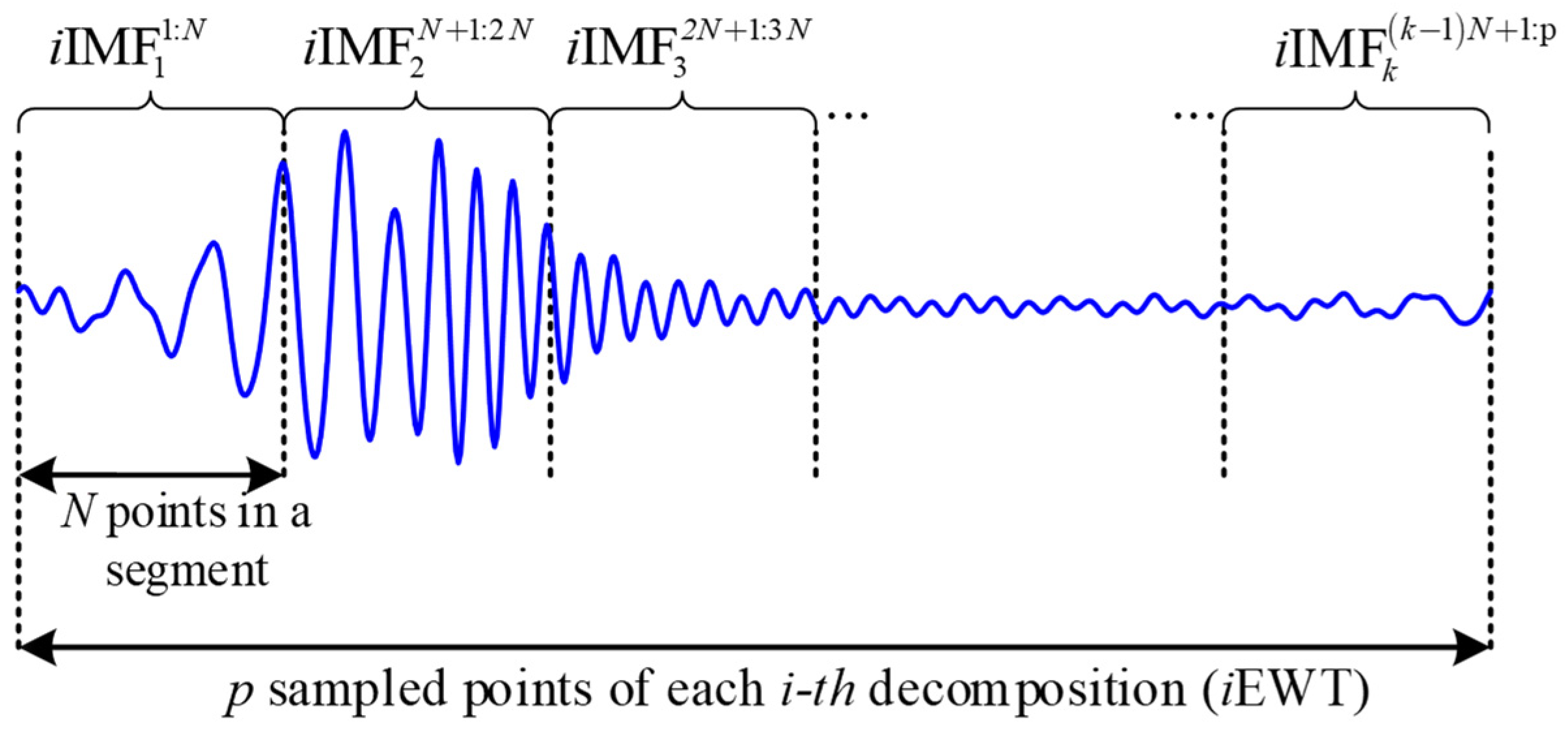
is segmented in equal parts, aiming to generate a consecutive set of samples. The segmentation is performed as
Figure 2 depicts; thereby, if each one of the i-th
is represented with a vector
with a total of
points, its segmentation in
equal parts is performed considering
points in each segmented part (
); in other words, the segmentation can be achieved by following the established Equation (2).
After applying the EWT and segmenting each resulting IMF, a characteristic high-dimensional feature matrix composed of 150 statistical time-domain-based features is estimated for each assessed condition. Specifically, for the conditions of HLT, 2SCTs, 4SCTs, and 6SCTs, the following feature matrices are generated:
,
,
, and
, respectively. Additionally, due to different operating frequencies also being considered to operate the IM at different rotating frequencies, the following feature matrices are computed for a particular condition (i.e., HLT):
,
,
, and
, respectively (for each operating frequency). Regarding the proposed set of statistical time-domain-based features, this set of features are used in this work due to having the capability of modelling trends and changes in signals, as well as their low computation burden facilitating their estimation, producing quick responses when implemented. The corresponding mathematical equations of these statistical features are summarized in
Table 1.
2.4. Feature Optimization and Modelling
The estimation of a high-dimensional set of features can contribute to the computation of representative and discriminant patterns that can be used to differentiate between different faulty conditions; however, the computation of non-useful and correlated information is also unavoidable and the performance of diagnosis may be affected during the fault assessment. In this regard, this work also proposes an optimization stage with the aim of discarding that insignificant information that can affect the performance of the diagnosis; thereby, this stage is focused on selecting and modelling the most representative information that preserves the topology of the data. Accordingly, this selection and modelling procedure is individually applied to each one of the considered conditions and it is achieved by means of a structure composed of a genetic algorithm (GA) and several self-organizing maps (SOMs). Hence, for each one of the assessed conditions, the GA-SOM structure will find a combination of several that preserves the topology of the data; under this criterion, the SOM archives the individual modelling of each considered condition.
It should be clarified that the SOM is an unsupervised neural network introduced by Teuvo Kohonen in 1986 [
35]; the objective of this network is to be able to represent a high-dimensional feature space in a coordinate system (neuron grid generally represented into 2
d) by means of a learning procedure. During this feature learning, the topology of the original feature space is preserved; that is, points that are close in the original feature space remain close in the reduced dimension space created. Thereby, the feature learning through SOM is performed by defining the input and output layer as depicted in
Figure 3; the input layer comprises
N neurons that represent the total of features of the input feature space
and the output layer consists of
M neurons that are predefined into a
grid. Thereby, the learning is carried out by mapping the high-dimensional feature space into a 2
d neuron grid through the connection of each input neuron
of the input layer to each neuron
in the output layer with a weight,
. As a result, in the SOM neuron grid are found the Best Matching Units (BMUs), where the BMUs are the nearest neurons from the output to the input layer. Certainly, the corresponding BMU associated with each input sample of the input feature space
can be determined by measuring the Euclidean distance following Equation (18), where
is a sample that belongs to the training input feature space
. To quantify the quality of adaptation achieved with the mapping through the SOM, the deviation between the BMUs and the input feature vectors is measured with two metrics, the quantization error (
) and the topological error (
), described with Equations (19) and (20), respectively. This is where each
represents each one of the features of the input feature space
, whereas each vector
jth in the output neuron grid is represented by
, and
is equal to 1 when the two first-evaluated BMUs for
are adjacent (are not close between them); otherwise,
is equal to 0.
In regard to the proposed feature optimization stage performed with the GA-SOM structure, it is individually carried out for each one of the tested conditions as is described in the following four steps:
Step i: The definition of the initial population of the GA is carried out by considering a logical vector that has 10 elements, and each element represents every one of the obtained IMFs (). Consequently, the population is randomly initialized and then evaluated; indeed, the first population is composed of at least one element or of the combination of different elements. It should be mentioned that each one of the elements represents each one of the IMFs and each corresponding IMF is in turn represented by its corresponding set of statistical features estimated in the previous subsection (2.3. High-Dimensional Feature Estimation). Afterward, Step ii is performed once the initialization of the population is performed.
Step ii: The evaluation of the initialized population is then achieved through the considered fitness function; for this proposal, the fitness function is based on the minimization of the quantization error () obtained with the mapping through the unsupervised SOM neural network. Exactly, the evaluates the quality of the resulting mapping in the output feature space, that is, how well the input feature space fits to the output space. Hence, the GA-SOM structure may solve an optimization problem where the solution is to find that combination of IMFs that gives the smallest value when such selected IMFs are modelled through the SOM. After evaluating the entire population, the best combination of IMFs is found and the procedure continues in Step iv.
Step iii: The operation of mutating is carried out with the roulette wheel selection and the GA creates a new population in terms of the last/old population; the generation of the new population is created by taking the chromosomes that lead to lower values in the fitness function. In fact, it is considered that the smallest values of the depict a high performance in the SOM modelling. Also, the Gaussian distribution is considered during the mutation procedure, and once this step is achieved, Step ii must be followed.
Step iv: The criteria to stop the GA are restricted by reaching a maximum defined number of generations and/or by solving the optimization problem, which is to find the combination of IMFs that produces a minimum value of the ; in other words, by finding the combination of IMFs that improves the modelling of each assessed condition in an individual way. Then, the process continues in Step iii.
After carrying out the optimization process through the GA-SOM structure, each considered condition is individually modelled with a specific unsupervised SOM neuron grid. That is, the high-dimensional set of statistical features that represents each considered condition is reduced and represented by four SOM neuron grids (, , , and ) that model the behavior of the IM under different severities of SCTs.
2.5. Feature Reduction and Fault Detection
In the last stage, the use of the Linear Discriminant Analysis (LDA) technique is first considered in order to perform the compression of the whole resulting SOM neuron grid models (, , , and ). Moreover, such compression is also performed with the aim of projecting all considered conditions in a unique 2d space while the predefined number of neurons () of each SOM neuron grid is also reduced. Hence, the LDA, which is a technique supported with a linear transformation that aims to maximize the linear separation between considered conditions (classes), leads to emphasizing the most discriminant information, and the obtained 2d projection is a representation of the input feature space in different weights. The reduction by means of the LDA also influences the task of classification; thus, the classification is facilitated due to each class represented by the new extracted features in the 2d plane, ideally appearing as separated from each other.
Finally, the fault detection is performed with a neural network (NN)-based classifier; the structure of the NN consists of only three layers, where the number of neurons used in the input, hidden, and output layers is equal to 2, 10, and 4, respectively. Accordingly, in the input layer is the evaluation of the set features extracted with the LDA technique (coordinates of the 2
d projection), the definition of the hidden layer is according to suggestions made in the literature [
36], and the output layer may activate a corresponding neuron, which is associated with the detections of a specific condition (HLT, 2SCTs, 4SCTs, and 6SCTs). During the training and validation of the proposed NN, a feedforward scheme is considered, and a
k-fold cross-validation scheme with the objective of obtaining statistically significant results, as well as the use of the sigmoid function as the activation function for posterior evaluation of the corresponding membership function.
4. Results and Discussion
The proposed methodology for detecting the occurrence of different severities of ITSC in an IM is developed in Matlab R2022a, and this is a specialized software that has been used in several applications of engineering and other areas. Regarding the proposed method, it is validated under real data acquired through several experiments from a laboratory test bench; thus, as previously stated, the three stator current signatures () of the IM are continuously monitored during the iterative evaluation of the HLT, 2SCTs, 4SCTs, and 6SCTs’ conditions in the start-up transitory regime. Additionally, it must be emphasized that each studied condition is tested under four different operating frequencies (15 Hz, 30 Hz, 50 Hz, and 60 Hz) through the VFD; thus, the acquisition of the start-up transitory regime consists of recording the first 5 seconds where the first 3 seconds belong to a linear starting ramp that reaches the set frequency, for each corresponding supply frequency. The stator signatures are acquired with a sampling frequency of 6000 Hz; consequently, 30 k samples are continuously acquired and stored for a further analysis.
Afterward, the high-dimensional feature estimation is carried out by means of applying the EWT and by estimating the proposed set of statistical features; in this sense, only the first current line (
) is considered to be analyzed to achieve the fault diagnosis. Thereby, for each considered condition, its acquired stator current signature is processed with the EWT and as a result, a set of decompositions are obtained that are also known as the IMFs allowing the MRA. In
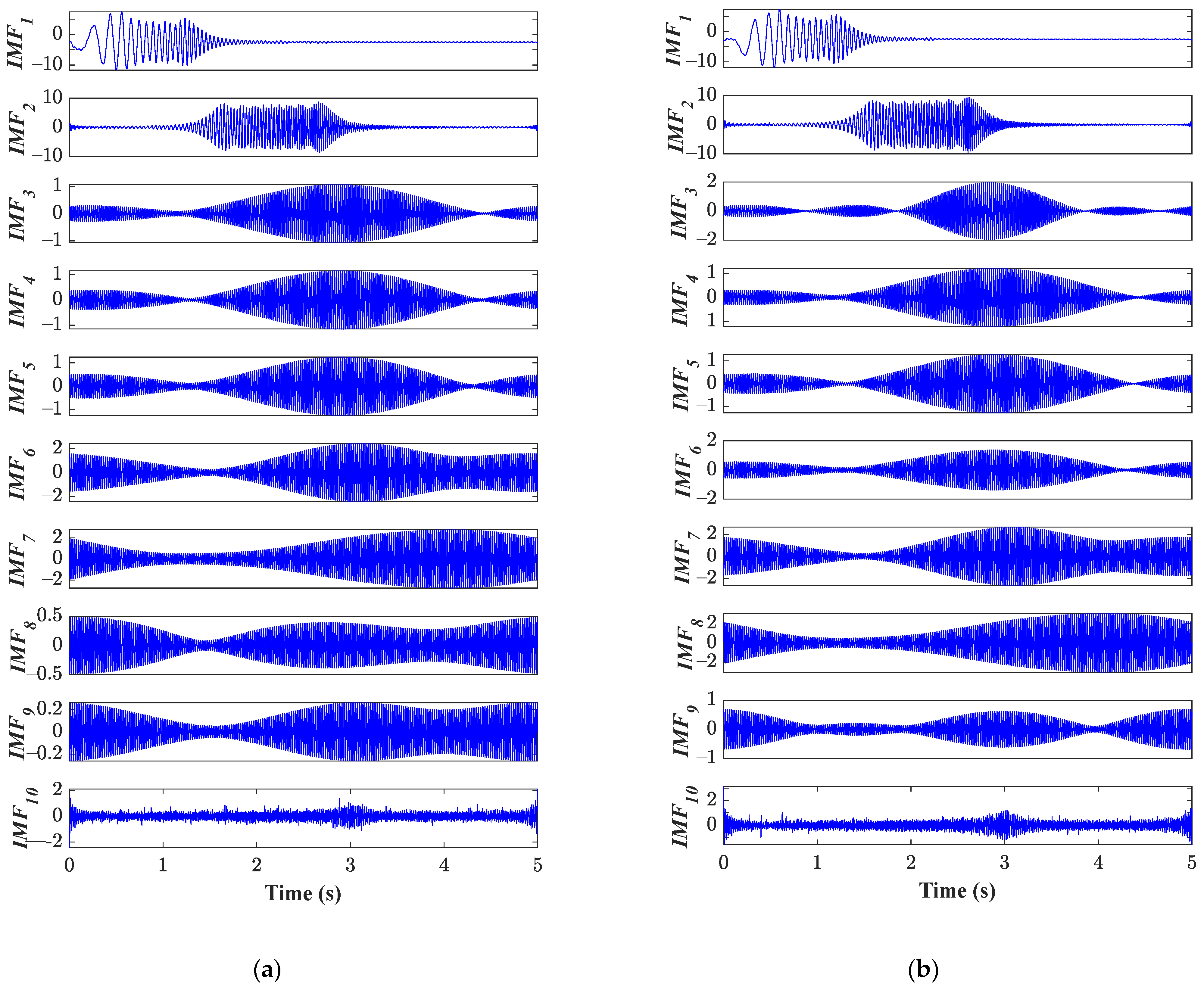
Figure 6, the first ten IMFs are shown (
), obtained when the stator current signature of the HLT and 6SCT conditions is processed through the EWT; as appreciated with a visual inspection, there are several differences that are between each corresponding IMF; indeed, the most important differences belong to qualitative changes that are associated with the shapes of each IMF. Certainly,
,
,
,
, and
depict important changes that are associated with IM behavior due to the tested conditions. Although
Figure 6 shows only the IMFs obtained from the current signature for the HLT and 4-SCT in the IM, it should be mentioned that the degradation of the stator winding of the IM may also produce changes that mainly affect the stator current consumption; thus, all changes and/or modification introduced with the occurrence of SCTs may lead to obtaining different shapes in the IMFs when the current signal is processed with the EWT. Once the processing through the EWT is carried out for each assessed condition, each one of the generated IMFs is then subjected to the segmentation procedure as previously explained in
Section 2.3.
High-Dimensional Feature Estimation. Hence, each IMF that consists of 30k data points is divided into 100 equal parts in order to generate a consecutive set of samples; then, from each part is estimated the set of statistical time-domain features (
Table 1). Accordingly, four high-dimensional feature matrices are generated as the matrices that characterize the behavior of the IM under different conditions; the matrices are composed of 150 statistical features or columns (15 features per IMF) and are denoted as
,
,
, and
, for each considered condition. Regarding the number of samples or rows, it should be remembered that each studied condition is tested under four different operating frequencies (15 Hz, 30 Hz, 50 Hz, and 60 Hz); therefore, each one of the characteristic matrices is composed of the concatenation (as a row) of the characteristic feature matrices estimated for all tested frequencies; that is, for example, for the HLT condition,
.
Later, the previously estimated matrices
,
,
, and
are optimized by means of a GA-SOM structure; despite representative and discriminant information being allocated in the high-dimensional feature matrices, the non-useful information and/or correlated information is also estimated. In this sense, the main objective of the GA-SOM structure involves selecting that representative information that can be used for an efficient data modelling; such an optimization procedure is carried out as described in
Section 2.4, and more details are given below:
The optimization and modelling process is performed in an individual way for each one of the assessed conditions; hence, each one of the feature matrices , , , and are individually subjected to this procedure.
When analyzing one feature matrix (i.e., ), the optimization starts by defining an initial population with 10 elements in the GA; such a population is represented by a logical vector, and it is randomly initialized. For example, if the initial population is represented by the vector 1 0 0 1 1 0 0 0 0 1, it can be understood that each true value in the logical vector represents the following IMFs: , , , and .
The GA continues its operation by evaluating the initial population into the fitness function, as well as mutating; and these steps are performed and repeated until the optimization problem is solved and/or the generations are reached. In regard to the fitness function, the true values in the logical vector of the populations indicate which one of the whole IMFs may be considered to be modelled using a SOM neuron grid; in fact, the modelling of the selected IMFs is performed in terms of their corresponding statistical features. That is, only the statistical features that belong to the IMFs are modelled using the SOM.
During the feature modelling, the SOM produces a numerical measure that represents the quality of the mapping procedure; hence, the value is taken into account as the metric to be minimized in order to guarantee the correct modelling of the data. As stated, the smallest values on the are associated with a proper mapping from the input to the output feature space; thereby, minimizing the is guaranteed to preserve the topology of the data.
As a result, the selection of a set of IMFs is carried out for each condition; in
Table 2, the set of selected IMFs are summarized for each studied condition, as well as the obtained
and
values also being included. Thus, the selected IMFs are then used to carry out the data modelling by means of the SOM network, and as previously mentioned, the SOM structure is predefined with a neuron grid that consists of 10 × 10 neurons; indeed, during the modelling of the selected IMFs, the
and
values depict small values. On the other side, the increase in the
value can be associated with deviations that occur whether the HLT condition is considered as the reference.
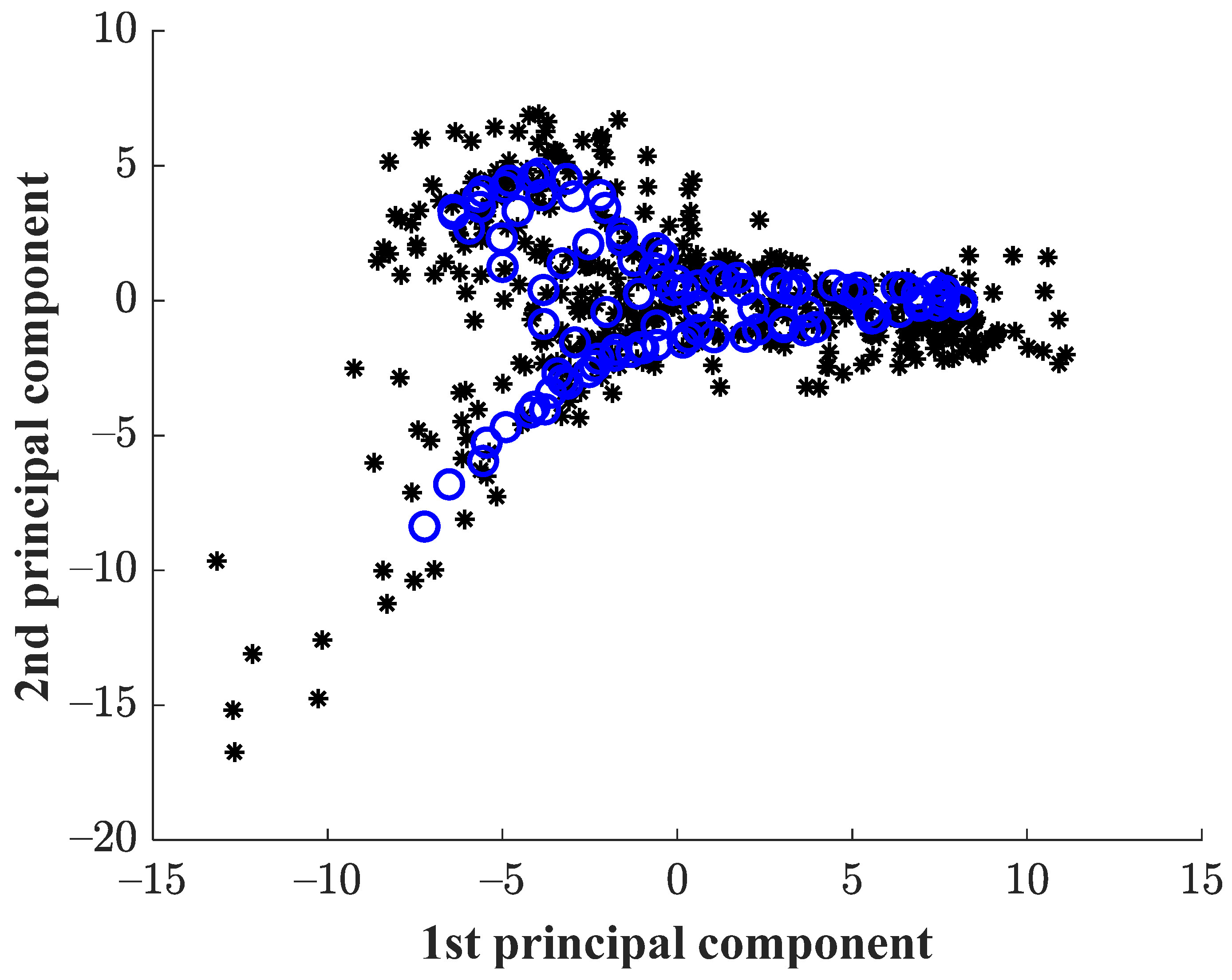
In order to demonstrate the effectiveness of modelling through the SOM structure,
Figure 5 shows the data distributions achieved by applying the Principal Component Analysis (PCA) over the original statistical features that belong to the selected IMFs, and by applying the PCA over the resulting modelled SOM neuron grid. As observed in
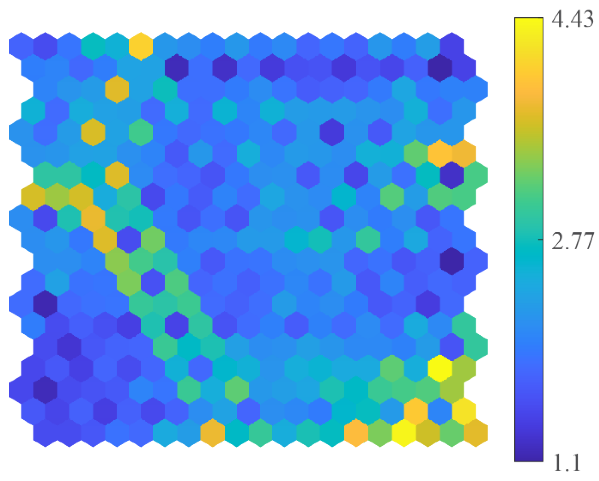
Figure 7, the distribution of the HLT data presents a particular shape whereas the distribution of the HLT SOM data adopts the same shape of the original data; indeed, through the modelling using the SOM network, the topological properties of the original feature space are preserved. Also, the modelling of each considered condition through the SOM leads to the representation with the U-Matrix, which is a 2
d grid that shows the distances between weight-vector-adjacent neuron units in the defined two-dimensional map. In
Figure 8, the resulting U-Matrix is shown that is computed during the modelling of the HLT condition and represents the distances between the trained neurons; from
Figure 8, it should be mentioned that the darkest areas belong to data concentrations (small distances between neurons) whereas the lightest areas may describe boundaries (large distances between neurons). Thereby, from the optimization and modelling stage, the following SOM neuron grids are obtained:
,
,
, and
.
Subsequently, the dimensionality reduction in the obtained SOM neuron grids (
,
,
, and
) is carried out by using the LDA technique; in the feature reduction, the whole SOM neuron grids are considered and their original feature spaces are subjected to a space transformation through a linear combination; as a result, the 2
d visual representation is obtained as is shown in
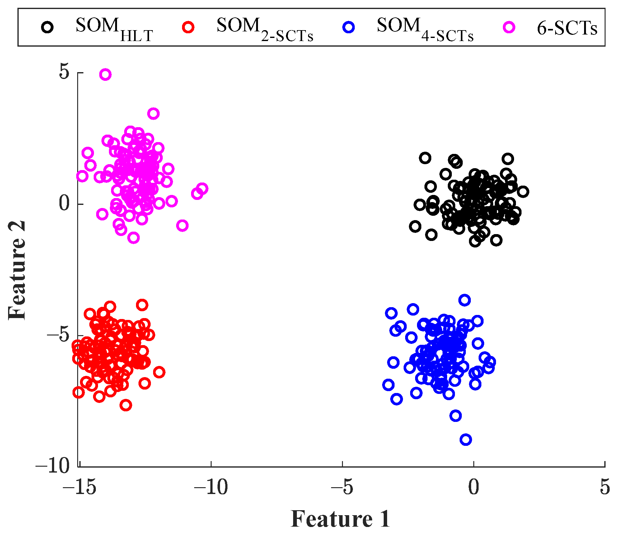
Figure 9. As it is appreciated, all the assessed conditions appear as separated from each other, and such separation is in part from considering the processing of the stator current signal through the EWT and then the characterization of each obtained IMF by calculating the proposed set of statistical features. The LDA leads to extracting a new set of features (Feature 1 and Feature 2) and these features represent the linear combination of the original feature space; the combination is carried out with different weights where the large weighting values represent relevant or discriminative information and small values depict non-relevant information. Another advantage of using the LDA is that the classification task is facilitated to the classification algorithm; hence, the fault detection is achieved with a single NN structure that comprises three layers. In the hidden layer, the extracted features are evaluated (Feature 1 and Feature 2); the hidden layer is defined with 10 neurons and the output layer is composed of 4 neurons, and each neuron in the output layer is associated with each one of the studied conditions (HLT, 2SCTs, 4SCTs, and 6SCTs). The training and validation of the NN-based classifier are carried out under a 5-fold cross-validation scheme with the sigmoid function as the activation function; also, 50 epochs are taken into account for the training of the NN. The resulting classification ratios achieved for the training and test of the NN are about 100%, for both cases;
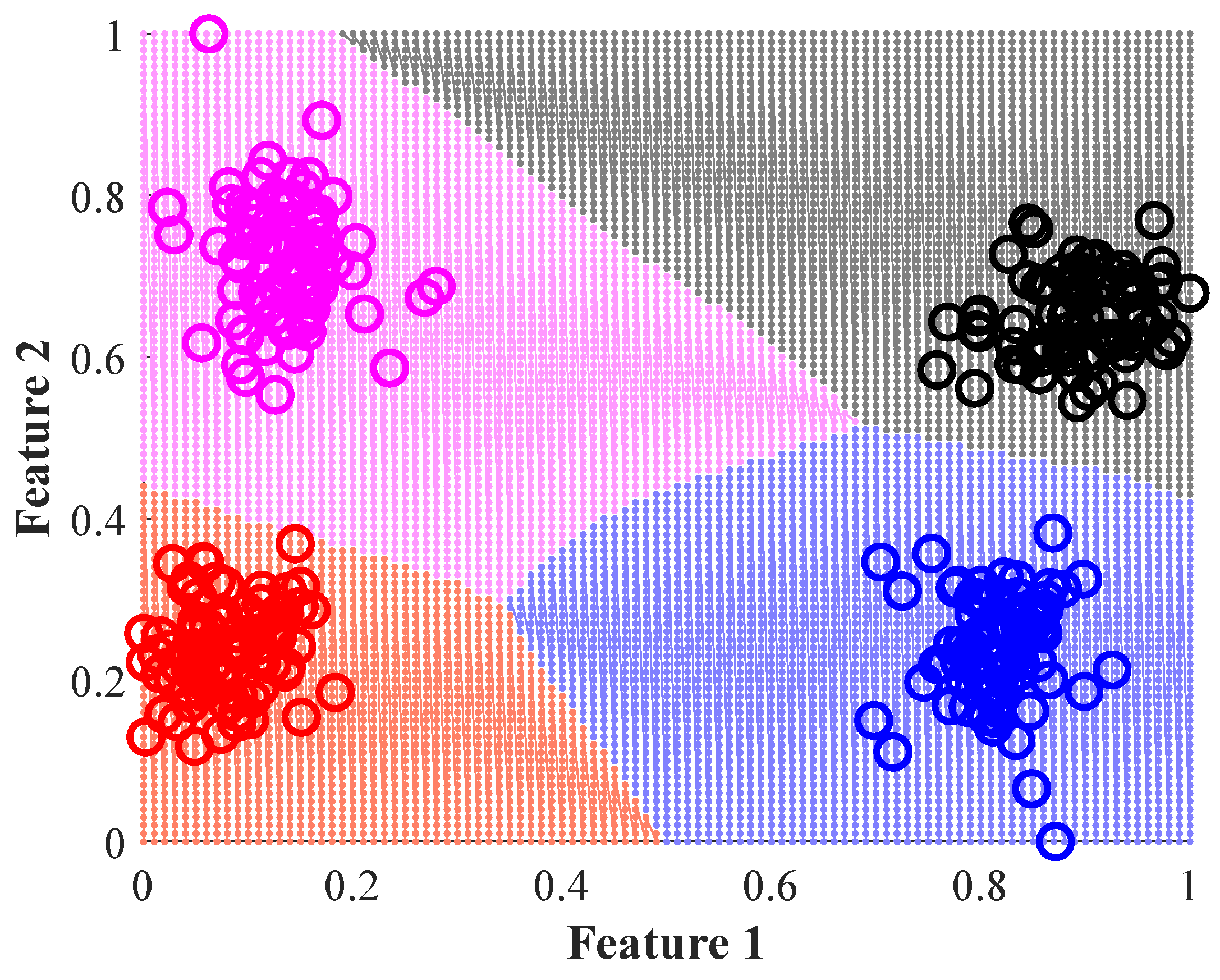
Table 3 summarizes the individual classification ratios. The high-performance classification ratio is due to the extracted features with the LDA showing a perfect separation between considered classes; as a consequence, the classification algorithm gives a maximum performance of 100%. Moreover, the NN classifier also facilitates the modelling of the decision regions as
Figure 10 shows, and during the training and validation of the NN, misclassifications and problems are avoided; however, the evaluation of the membership function can be considered in case of misclassifications.
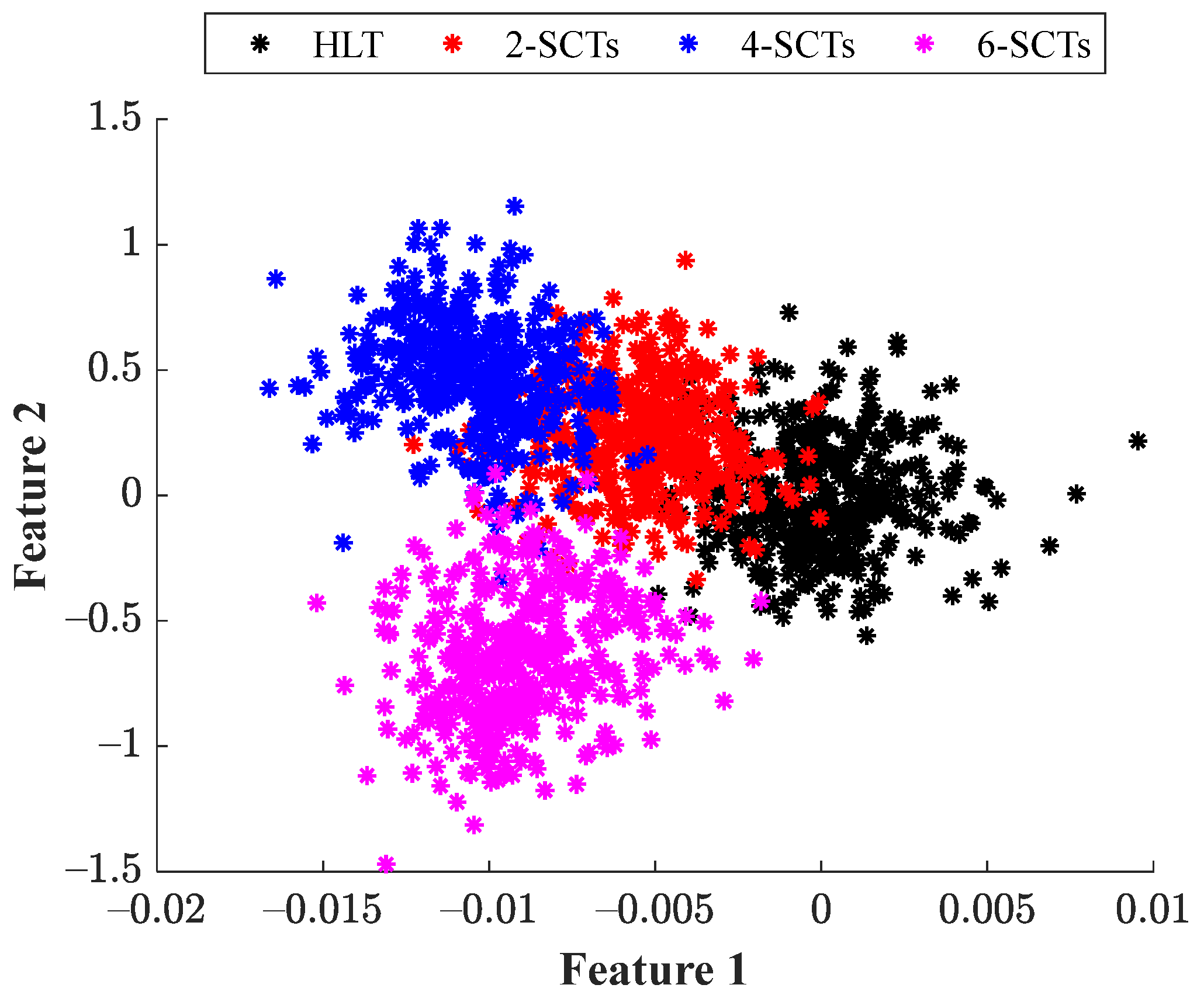
On the other side, in order to highlight the effectiveness of the proposed method, the same set of statistical time-domain-based features are also estimated from the three stator current signatures. That is, signals
are characterized by the computation of 15 statistical features, and to estimate these features, Equation (2) and
Figure 6 are also considered for the segmentation of the signals in 100 equal parts. As a result, three characteristic feature matrices are obtained for each one of the studied conditions; hence, a total of 45 statistical features are estimated to characterize the start-up transient behavior of the IM. Then, the 45 statistical features are subjected to the dimensionality reduction by means of the LDA and the resulting projection is presented in
Figure 11. As appreciated, four main clusters appear in the resulting projection but, although it is possible to distinguish each cluster, there is a considerable overlapping between all considered conditions, leading to the misclassification problems. Finally, the same structure of the NN-based structure is used to evaluate the extracted features of
Figure 11, and the global classification ratio achieved with the same NN is about 90.8% and 86.2% during the training and validation when the statistical time-domain features estimated from the stator current are subject to the reduction procedure with the LDA. Thereby, the results obtained with the proposed diagnosis methodology demonstrate the effectiveness of detecting the occurrence of SCT in an IM; moreover, the proposed method shows the advantage of being capable of assessing SCT faults under different operating frequencies. The proposed method can be implemented as a part of condition-monitoring strategies in industry, and the detection of SCT in an early stage may avoid unwanted stoppages.
The obtained results show the effectiveness of the proposed method for detecting the occurrence of different severities of SCTs during the start-up transient regime in an IM; indeed, the achieved high-performance classification ratio is mainly due to the capability of the proposed techniques (EWT and SOM) to characterize the transient stator current behavior and due to the ability to reduce high-dimensional feature spaces by retaining its topology. Similarly, the implementation of the LDA leads to facilitating the classification task since the structure and configuration of the NN-based classifier do not involve a high degree of complexity, consequently. Finally, to validate the structure and configuration of the proposed NN-based classifier, the features of
Figure 9 and
Figure 11 extracted by applying the LDA to the whole SOM neuron grids (
,
,
, and
) and applied to 45 statistical features estimated from raw current signatures, respectively, are evaluated under a multi-class support vector machine (MC-SVM) that achieves the classification under a one-against-all scheme. Thereby, the configuration of the MC-SVM considers a radial basis function (RBF) as the kernel function with an automatic scale adjustment, and the value of the box constraint (
) is set with values such as
. The training MC-SVM classifier is used by holding out 80% of the data sets and the remaining 20% is used for validation purposes; thereby, the average classification ratios for the training and validation are 87.8% and 83.9%, respectively, for the features extracted with the LDA of
Figure 9 and
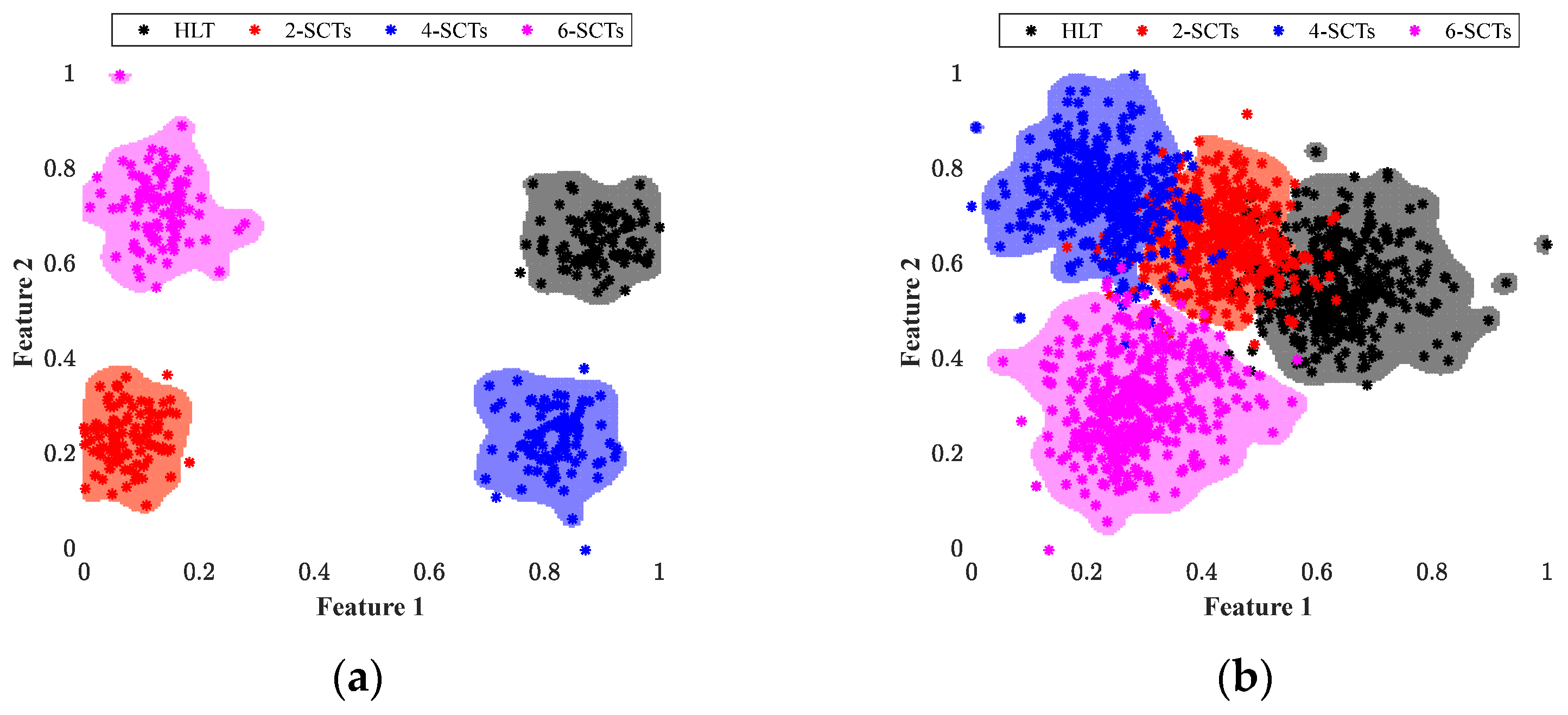
Figure 11. The modelling of the classification regions is also estimated with the MC-SVM; thus,
Figure 12a,b show the resulting decision regions achieved with the MC-SVM under a one-against-all scheme. Although the decision regions of
Figure 12a show a good fit with the data of each considered condition, the modelling of undesired regions is unavoidable (a small region in the upper left corner), as well as several samples being outside of their corresponding boundaries. On the other side, the decision regions of
Figure 12b show a clear overlapping between them, and the overlapping is a critical issue that is produced with the one-against-all scheme due to a particular region that can be modelled with more than one class (condition). Therefore, the proposed NN-based classifier represents a practical solution with an excellent tradeoff between structure complexity and classification performance. Moreover, although NN-based classifiers can be sensitive to outliers that are inherent to the data, this issue can be minimized by considering the normalization of the data to reduce the impact of outliers in the network.
It must be mentioned that there are some other methodologies that also allow for identifying an incipient ITSC fault. For instance, in [
37], a technique is presented that uses an Instantaneous Symmetrical Component Analysis and a frequency feature extraction based in Fourier Transform. A SOM modeling stage is also used to characterize every fault condition; however, an optimal feature selection is not performed, nor a feature reduction, and they obtain classification rates around 95%. In this sense, it is demonstrated that the feature optimization along with the LDA feature reduction allow for increasing the effectiveness in the classification task. Moreover, when FT is used, it is not possible to perform an analysis during the start-up transient since FT is a technique for a steady-state analysis. Some other works propose the analysis of variables different from the stator current like vibrations or stray flux [
21,
38]; those works also report accurate results but, again, they work in a steady state while the proposed approach is able to deliver results during the transient start-up.
Competency of the Method in Front of the Detection of Other Faults
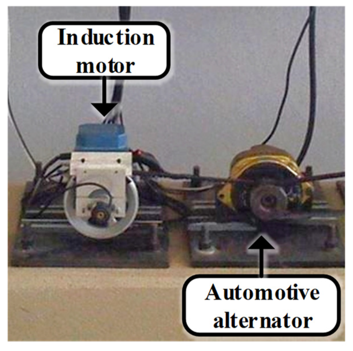
Moreover, with the objective of extending the validation of the proposed method to detect other types of faults during the start-up transient regime of the IM, the proposed diagnosis methodology was applied to another experimental data set, which contains information related to the occurrence of two conditions of Broken Rotor Bars (BRBs). The data set consists of three stator current signatures acquired from another experimental test bench that is composed of a 0.735 kW three-phase IM coupled to an automotive alternator (load) by means of a pulley-belt system;
Figure 13 shows a picture of the experimental test bench where the two conditions of BRB are evaluated. In the IM, a healthy (HLT) condition and two severities of BRB, specifically one and two BRBs (1BRB and 2BRB), are tested; thereby, the acquisition of the stator currents (
,
, and
) of the IM was performed with the same DAS and a similar set of hall-effect current sensors with a sampling frequency of 6 kHz. In fact, each considered condition is iteratively tested in the IM under two different operating frequencies (50 Hz and 60 Hz) and the data are acquired several times during the first 5 seconds in the start-up transient regime of the IM.
Afterward, the proposed method was applied as follows:
Step i and ii: These two first steps were previously performed since they are based on the definition of the electromechanical system under inspection and considered the stator current acquisition.
Step iii: To generate the high-dimensional set of features, only the first line current (
) is considered for processing through the EWT; hence, a total of ten intrinsic mode functions (
) or decompositions are achieved after applying the EWT to the line
for each considered condition.
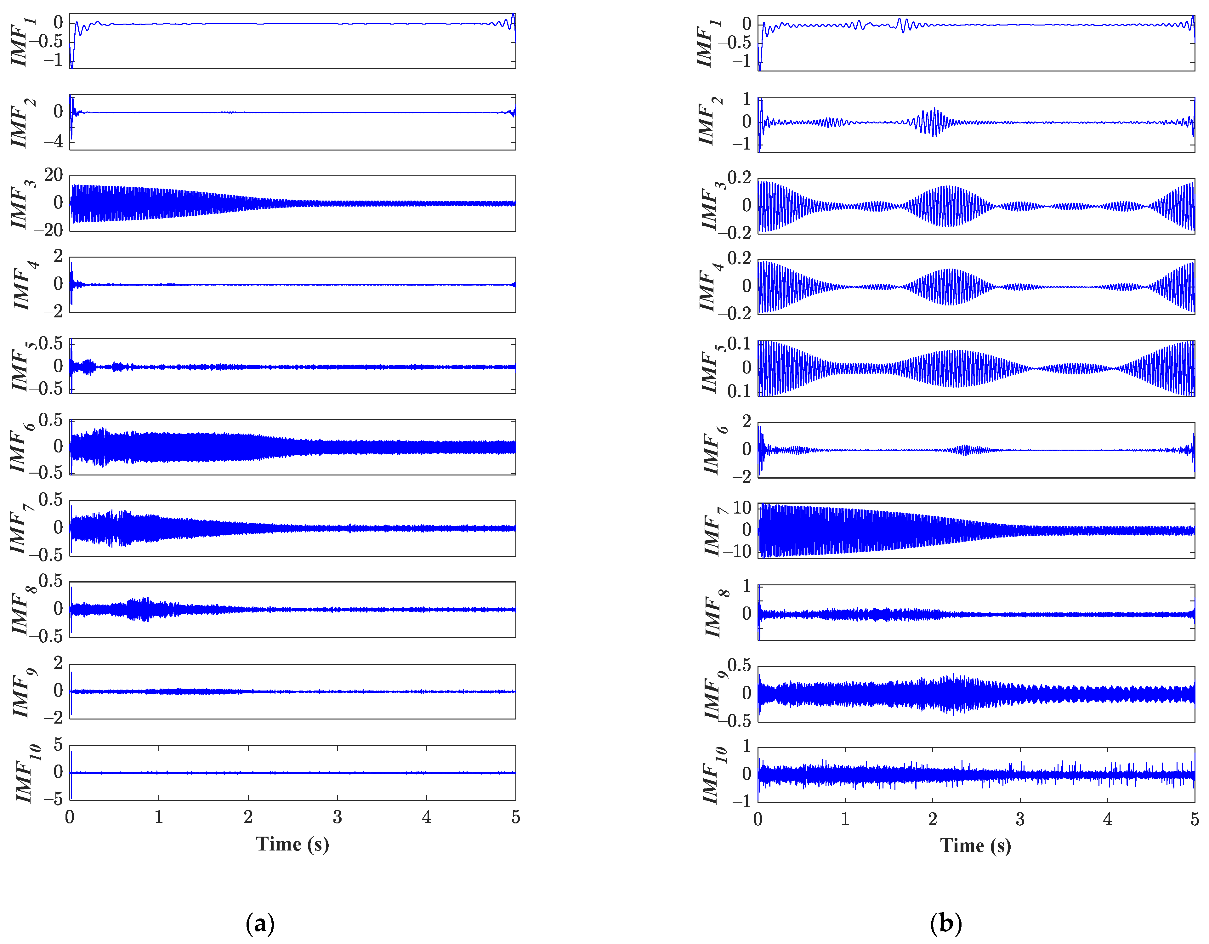
Figure 14a,b show the decomposition obtained with the EWT when applied to the line
when the IM operates under the HLT and 2BRB, respectively. As observed, there are significant differences between each one of the
, but the most important changes that can be associated with behavior of the IM in the start-up regime are in the
,
,
,
, and
. It can be assumed that changes and modifications in the
are due to the influence of BRBs in the IM that commonly introduce additional components in the stator current lines at
. Subsequently, the characterization of each one of the achieved
is carried out; that is, each
is segmented into 100 equal parts to create a consecutive set of samples and from each segmented part, the proposed set of 15 statistical time-domain-based features is estimated. As a result, for each considered condition, the feature matrices
,
, and
are respectively generated for each condition (HLT, 1BRB, and 2BRB).
Step iv: The feature optimization is performed with the proposed GA-SOM structure; particularly, the GA-SOM structure may find a combination of that produces a minimization of the value when the chosen/selected are evaluated through a particular neuron grid SOM model. During the feature optimization, the following sets of IMFs are selected as the best that minimize the value: , , , , , and for the HLT condition; , , , , , and for the 1BRB condition; and , , , , , and for the 2BRB condition. Once the optimization procedure is accomplished, the individual modelling of each one of the conditions under evaluation is carried out and three resulting SOM neuron grid models are obtained (, , and ). The value for the HLT condition was around 3.65 whereas for the conditions of 1BRB and 2BRB, it was around 19.38 and 34.91, respectively; on the other side, the value shows an average value of approximately 0.07 ± 0.015, for all conditions.
Step v: By means of the LDA technique, the resulting SOM neuron grids are subjected to a compression procedure with the aim of reducing its original dimension given with the predefined number of neurons (
), as well as for projecting all considered conditions in a unique 2
d space. From the dimensionality reduction achieved with the LDA, a new set of features is extracted (2
d projection); then, the new extracted features are evaluated in an NN-based classifier to obtain the automatic fault diagnosis. The structure of the NN classifier consists of three main layers where 2, 10, and 3 neurons are the numbers of neurons in the input, hidden, and output layer.
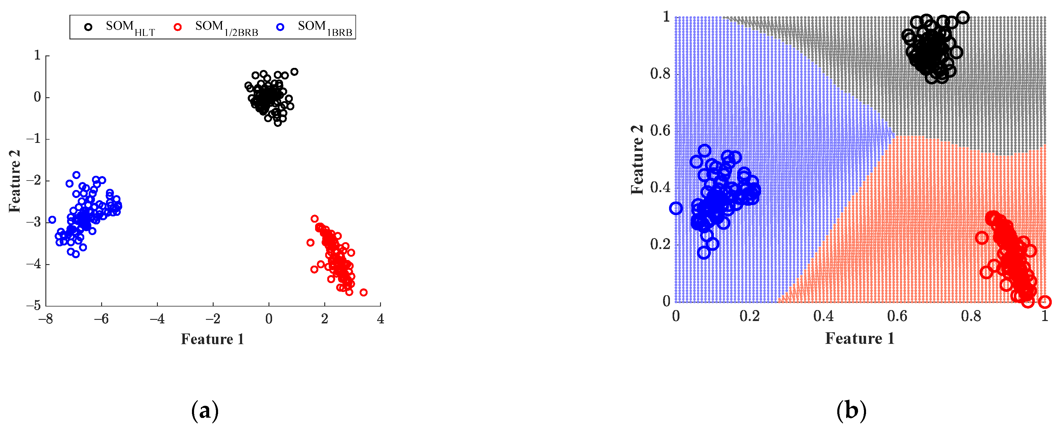
Figure 15a shows the resulting 2
d projections obtained after applying the LDA to the SOM neuron grids that model each one of the assessed conditions (
,
, and
); as appreciated, a clear separation between considered conditions is obtained. The separation between considered conditions is in part due to the capability of the EWT to extract a set of IMFs that characterizes the behavior of the IM in the start-up regime, as well as due to the potentiality of the statistical time-domain-based features to model changes and trends in signals and also due to the advantage of SOM to reduce high-dimensional data sets by preserving the topology. On the other hand,
Figure 15b shows the resulting classification regions achieved with the proposed NN-based structure, and it is worth mentioning that during the training and test, a global classification ratio of about 100% is reached. The classification task performed with the NN facilitated due to whole processing applied to the data. The obtained results prove the capability of the proposed method for detecting different types of faults that can occur in IMs; specifically, the method can deal with the detection of different severities of SCTs and different severities of BRBs, and such detection is carried out in the start-up regime of the IM and the method leads to effective results regardless of the operating frequency.


 ,
, 


