A Fault Tolerance Method for Multiple Current Sensor Offset Faults in Grid-Connected Inverters

Abstract

Three-phase grid-connected inverters have been widely used in the distributed generation system, and the current sensor has been applied in closed-loop control in inverters. When the current sensor offset faults occurs, partial fault features of multiple current sensors disappear from the closed-loop control grid-connected system, which leads to difficulties for fault diagnostics and fault-tolerant control. This paper proposes a fault tolerance method based on average current compensation mode to eliminate these adverse effects of fault features. The average current compensation mode compensates the average of the three-phase current to the αβ axis current to realize the fault feature reconstruction of the current sensor. The mode does not affect the normal condition of the system. Then, the data-driven method is used for fault diagnosis, and the corresponding fault tolerant control model is selected according to the diagnosis results. Finally, the experimental results show that the proposed strategy has a good fault tolerance control performance and can improve the fault feature discrimination and diagnostic accuracy.

1. Introduction

With the continuous increase of energy demand, distributed power generation systems of renewable energy have been rapidly developed. The grid-connected inverter is an essential interface between the distributed power generation system and the utility grid. In various topologies of grid-connected inverters, cascaded H-bridge multilevel inverters (CHMI) have the advantages of low harmonic content, fewer switching losses, and modular structure. So, they have been widely used in renewable energy grid-connected systems such as photovoltaic or wind energy systems. There are two primary sources of faults in a grid-connected inverter, namely, electrical and sensor faults. Electrical faults generally include open-circuit faults and short-circuit faults of power switches [1]. Protection of short-circuit faults is usually based on hardware circuits. Most researchers concentrate on open-circuit faults [2,3,4,5]. In addition to this, sensors provide real-time information for the closed-loop control. The precise data provided by sensors have an important impact on the control performance of the system [6]. Thus, the fault-tolerant system proposed in this paper is mainly focused on multiple current sensor faults. To improve the system’s stability and safety in the case of a sensor fault, it is necessary to accurately locate the fault and activate the appropriate fault-tolerant control method [7,8].

A qualified fault-tolerant control system needs highly accurate fault diagnosis results to prevent the secondary failure caused by choosing the wrong fault-tolerant control mode. The fault identification and diagnosis methods can be categorized into model-based methods [9], signal-based methods [10], and data-driven methods [11]. Compared with the other two methods, the data-driven methods have higher generalization capability and robustness for complex systems [11,12,13,14,15]. These methods do not need an accurate mathematical model of the system. They can only establish the mapping from fault characteristics to fault category labels through historical fault data. In data-driven fault diagnosis methods, various signal processing methods and fault feature extraction methods are usually used to amplify the fault features. In [11,12], Fourier transform and Wavelet transform are used to process the original signals, respectively. Fourier transform can extract the information in the frequency domain, but the information in the time domain is totally lost. Wavelet transform can analyze the signal in the time-frequency domain and obtain more fault information [13]. As for fault feature extraction methods, [14] uses principal component analysis to extract the fault characteristics of voltage in the frequency domain. The ReliefF algorithm is adopted to find the most correlated features in [15]. The purpose of these two methods is different. The former requires the extracted features to retain as much information as possible, while the latter requires the extracted features to be more conducive for their classification.

Most data-driven based methods studying feature extraction and diagnosis are based on given monitoring signals. Compared with numerous fault feature extraction algorithms, few papers focus on selecting effective monitoring signals. A fault-relevant variable selection method is proposed in [16], a genetic algorithm selects the best variable set for each fault, and a PCA model is established for each variable subset. In [17], multiple cost functions are introduced to measure the difference and contribution of original signals under different faults. In [18], a minimal redundancy maximal relevance algorithm is used to select the most representative variables for each subblock in the distributed framework. These methods select the best monitoring signals for fault diagnosis by establishing the corresponding evaluation indexes.

These methods are mainly applied to large-scale dynamic processes that are difficult to establish mathematical models for. The mathematical model of a grid-connected inverter can be established, but it is difficult to determine the precise parameters. In application scenarios where the modeling is complex, the selection of monitoring signals is generally based on the correlation of each variable and the target variable [18,19,20]. In the case where a precise mathematical model such as a grid-connected inverter is available, it is significant to propose a new method to select the appropriate monitoring signals.

In recent years, several sensor fault-tolerant control methods in power electronic converter systems have been proposed [19,20,21,22]. These methods can be divided into observer-based methods and signal compensation methods. The advantage of the observer-based method is that it can quickly and accurately locate the faults and realize the fault-tolerant control. In [19], aiming at the faults of different sensors in a motor drive, the fault diagnosis and fault-tolerant control are realized by estimating the angular velocity, establishing a stator flux observer, and decomposing the vector current. In [20], three independent observers are established in a motor drives system to realize the fault-tolerant control of one to two sensor fault conditions. The establishment of the observer requires an accurate mathematical model. However, CHMI have many power switches that make it difficult to build an exact mathematical model. The realization of the signal compensation method does not rely on a particular mathematical model, which is more suitable for CHMI. A new fault location and compensation strategy is proposed in [21]. The model and parameter-free compensators are proposed to recover the normal operation of the machine. This strategy completes the fault-tolerant control while significantly reducing the computation amount. In [22], the fault-tolerant control of current sensors is performed by reconstructing the three-phase current. When a current sensor experiences a fault, the fault-phase current signal is reconstructed through other healthy phase currents to keep the system stable. Although the above methods do not require the establishment of a complex mathematical model, they are only suitable for motor drive systems and single or two current sensor fault conditions. In addition, these methods also do not consider the impact of the closed-loop system on the fault features. In summary, the existing methods still have some shortcomings, and they are not suitable for the fault conditions of multiple current sensors in grid-connected systems using CHMI.

The diagnostic accuracy of the data-driven method is directly affected by the fault feature of the diagnostic signal. The current signal is greatly affected by the load and it is easily misdiagnosed [14]. Thus, the inverter output voltage is selected as the diagnostic signal [23]. However, the fault feature of the inverter output voltage will be affected by the current control system in grid-connected inverters. A current control system is required to make the output power quality reach the grid-connected standard [24]. In recent years, many control strategies have been proposed to eliminate the adverse effects caused by the unstable conditions in practical applications [25,26,27]. In order to improve the dynamic tracking performance, these control strategies are implemented in the synchronous dq or stationary αβ reference frames [28,29]. The transformation module of the original abc reference frame to the dq or αβ reference frame is directly connected to the current signal sensed by the current sensor. When a sensor fault occurs, the sensed current signal will have the corresponding fault feature. Due to the transformation module, the original fault feature will be modified and may disappear. If the initial fault feature disappears, the fault feature reflected in the output voltage will also have a low degree of discrimination. In this case, the fault diagnosis of three-phase grid-connected inverter will not be accurate, and the fault-tolerant control cannot be implemented. In summary, the existing methods still have some shortcomings, and they are not suitable for the fault conditions of multiple current sensors in grid-connected systems using CHMI.

In this paper, a fault-tolerant control strategy based on the average current compensation is proposed for three-phase current sensors fault of CHMI in grid-connected systems. The considered fault types of current sensors are offset faults. In our proposed strategy, an average current compensation is used to compensate and reconstruct the original fault features. For different fault conditions, a multi-mode fault tolerance control strategy is proposed to return the system from faulty condition to normal condition. Experimental results show that the proposed control strategy can effectively realize fault-tolerant control and improve the fault feature discrimination at the same time.

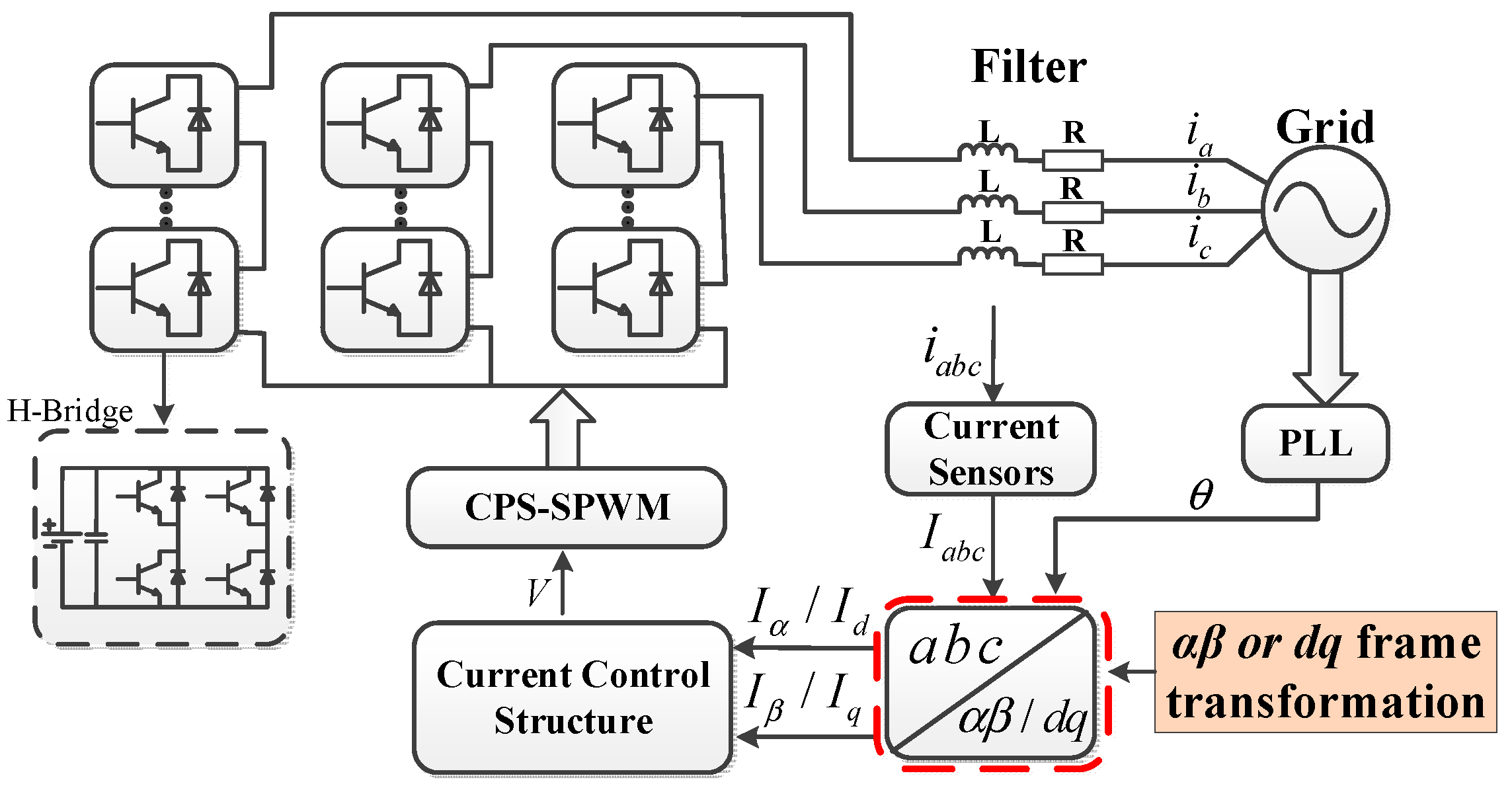
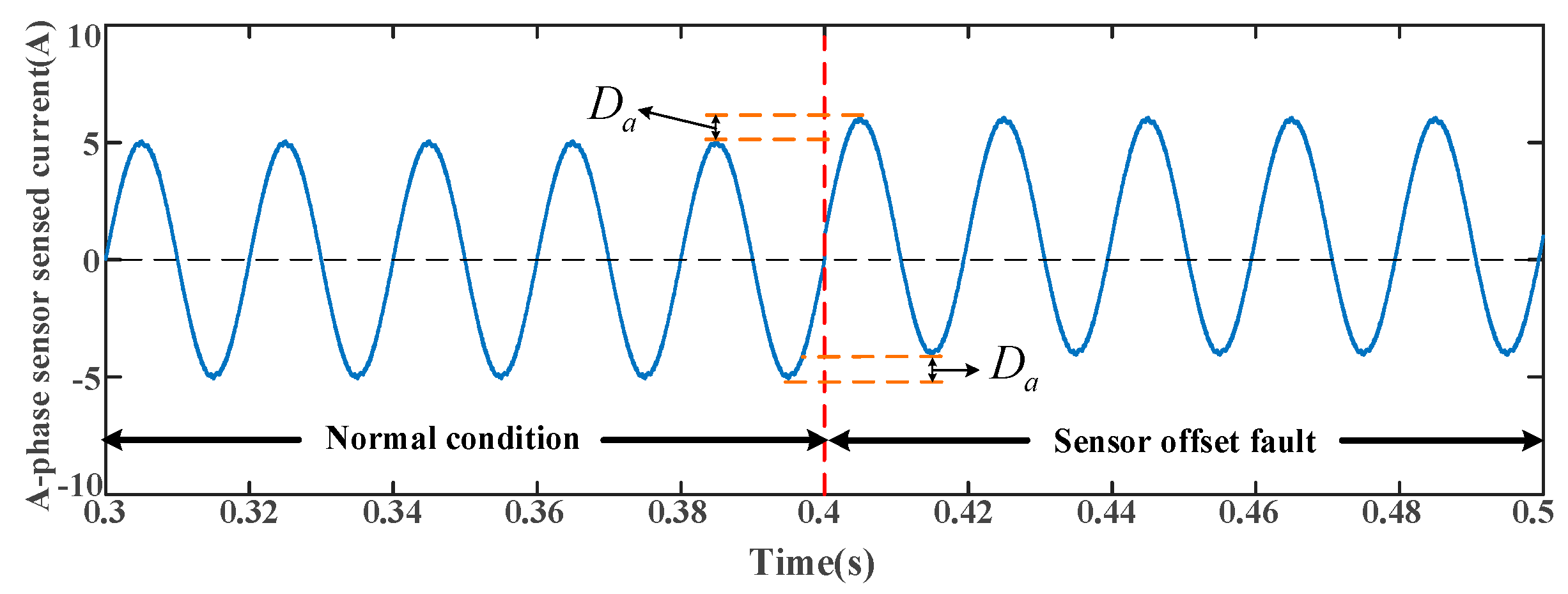
2. Problem Description

Figure 1 shows the block diagram of a three-phase 2n + 1 levels cascaded H-bridge multilevel grid-connected inverter. Each leg is composed of n H-bridge basic units. According to the grid information θ provided by the phase-locked loop (PLL), the three-phase grid-connected system transforms the sensed currents I_abc from the abc frame to the dq or αβ frame for tracking and control. Through the current control structure, the modulation voltage V can be obtained. According to the modulation voltage V, the Carrier Phase Shifting SPWM (CPS-SPWM) modulation technology is applied to generate the Pulse Width Modulation (PWM) signals to control the power switches. The inverter mathematical model can be established as follows:

$$L\frac{d{i}_{abc}}{dt}+R{i}_{abc}+e_{abc}=u_{abc}$$

(1)

where L, R, i_abc, e_abc, u_abc represent the filter inductance and its equivalent resistance, the grid current, the grid voltage, and the inverter output phase voltage, respectively.

Taking the traditional PI control system as an example, under the normal condition, the sensed current I_abc is equal to the grid current i_abc. The sensed current I_abc can be transformed in the dq and αβ frames by the following transformation modules:

$$T_{\alpha \beta }=2/3\cdot \left[\begin{array}{ccc}1& -1/2& -1/2\\ 0& \sqrt{3}/2& -\sqrt{3}/2\end{array}\right]$$

(2)

$$T_{dq}=\left[\begin{array}{cc}\cos \omega t& \sin \omega t\\ -\sin \omega t& \cos \omega t\end{array}\right]$$

(3)

The sensed current in the dq and αβ frames are derived as follows:

$$I_{abc}={[\begin{array}{ccc}{I}_a& I_b& I_c\end{array}]}^T$$

(4)

$$I_{\alpha \beta }=T_{\alpha \beta }{I}_{abc}=\left[\begin{array}{c}{I}_{\alpha }\\ I_{\beta }\end{array}\right]$$

(5)

$$I_{dq}=T_{dq}{I}_{\alpha \beta }$$

(6)

If the current sensors are faulty, the sensed current will have the corresponding fault feature. The fault features will also be transformed to the αβ or dq frame, and this process can make some original fault features disappear. The offset fault is a common sensor fault [30,31,32]. The adverse effect on the offset fault feature caused by frame transformation is discussed in the following.

In Figure 2, an A-phase sensor offset fault is set at 0.4 s. It can be seen that when an offset fault occurs, a fixed offset D_a appears in the sensor output current. The offset D_a makes A-phase sensed current unbalanced. In this state, fault features are clearly unobserved in the closed-loop control system. Then there may be an overcurrent in the circuit, causing damage to the grid-connected system. Defining the value of the offset generated by three-phase current sensors as D_abc [14], when an offset fault occurs, the sensed currents of three-phase sensors can be expressed as follows:

$$I_{abc}=i_{abc}+D_{abc}$$

(7)

where i_abc is the grid current under the normal condition.

Through the dq and αβ frames transformation modules, D_abc is transformed into the following forms:

$$D_{abc}={\left[\begin{array}{ccc}{D}_a& D_b& D_c\end{array}\right]}^T$$

(8)

$$D_{\alpha \beta }=T_{\alpha \beta }{D}_{abc}=\left[\begin{array}{c}{D}_{\alpha }\\ D_{\beta }\end{array}\right]$$

(9)

$$\left[\begin{array}{c}{D}_{\alpha }\\ D_{\beta }\end{array}\right]=\left[\begin{array}{c}2D_a/3-D_b/3-D_c/3\\ \sqrt{3}{D}_b/3-\sqrt{3}{D}_c/3\end{array}\right]$$

(10)

$$D_{dq}=T_{dq}{D}_{\alpha \beta }$$

(11)

The combination of different offset faults of the three-phase system will make the fault conditions more complicated. In these fault conditions, the values of three-phase offset can be identical, it is written as D_a = D_b = D_c. By substituting D_a = D_b = D_c into (10) and (11), we obtain:

$$\left\{\begin{array}{c}2D_a/3-D_b/3-D_c/3=0\\ \sqrt{3}{D}_b/3-\sqrt{3}{D}_c/3=0\end{array}\right.\Rightarrow \left\{\begin{array}{c}{D}_{\alpha \beta }=0\\ D_{dq}=0\end{array}\right.$$

(12)

According to (12), the offset fault feature is equal to zero in the αβ or dq frame when the values of three-phase offset are identical. In this case, the offset fault feature is eliminated due to the αβ or dq frame transformation module. For CHMI, the inverter side output voltages are used as the fault diagnosis signals. If the fault feature is equal to zero, the output voltages will be the same under the faulty and normal conditions, then the fault cannot be diagnosed and controlled. Therefore, effective fault characteristics should be obtained by analyzing the output signals.

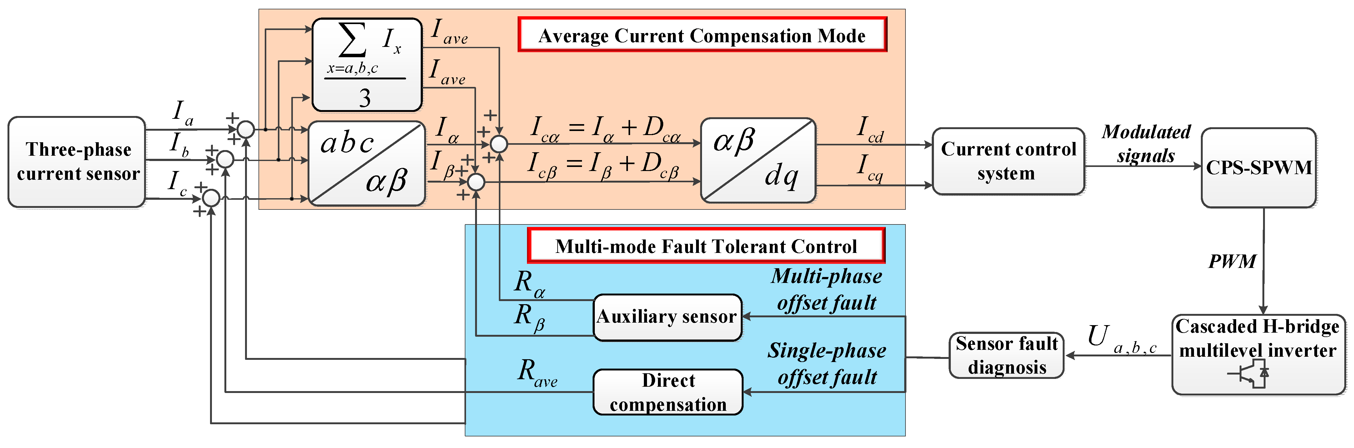
3. Multi-Mode Fault-Tolerant Control of Current Sensor Fault

To eliminate the adverse effects related to the traditional frame transformation and restore the distorted grid current under different sensor offset fault conditions, a fault-tolerant control strategy based on the average current compensation mode is proposed. The proposed strategy has two parts which are the average current compensation mode and multi-mode fault-tolerant control. The block diagram is shown in Figure 3.

3.1. Average Current Compensation Mode

As discussed in Section 2, the αβ or dq frame transformation may make the sensor fault feature disappear. In order to improve the discriminability of fault features and fault diagnosis accuracy, an average current compensation mode is proposed, which is shown in Figure 3. The function of the proposed strategy is investigated under different operating conditions.

3.1.1. Normal Condition

In the average current compensation mode, an average compensation signal of three-phase current is used to reconstruct the fault feature of current sensors:

$$I_{ave}=\frac{I_a+I_b+I_c}{3}$$

(13)

Under the normal condition, the sensed currents of sensors are equal to the grid currents, that is I_abc = i_abc. Therefore, (13) can be rewritten:

$$I_{ave}=\frac{I_a+I_b+I_c}{3}=\frac{i_a+i_b+i_c}{3}=0$$

(14)

Thus, the average current compensation mode will not affect the control system under the normal condition.

3.1.2. Offset Fault Condition

According to (7) and (13), when offset faults occur, the average of the three-phase sensed current is as follows:

$$I_{ave}=\frac{I_a+I_b+I_c}{3}=\frac{i_a+i_b+i_c}{3}+\frac{D_a+D_b+D_c}{3}=\frac{D_a+D_b+D_c}{3}=D_{ave}$$

(15)

Adding (15) to (10), the offset fault feature in the average current compensation mode can be expressed as follows:

$$\left[\begin{array}{c}{D}_{c\alpha }\\ D_{c\beta }\end{array}\right]=\left[\begin{array}{c}2D_a/3-D_b/3-D_c/3+D_{ave}\\ \sqrt{3}{D}_b/3-\sqrt{3}{D}_c/3+D_{ave}\end{array}\right]$$

(16)

$$\left[\begin{array}{c}{D}_{cd}\\ D_{cq}\end{array}\right]=T_{dq}\left[\begin{array}{c}{D}_{c\alpha }\\ D_{c\beta }\end{array}\right]$$

(17)

Compared with (10) and (16), it can be observed that the average current compensation mode adds a new feature D_ave to the original fault feature in the αβ frame. In the discussion of Section 2, the offset fault feature in the αβ frame is equal to zero when the value of three-phase sensor offset is identical (D_a = D_b = D_c). In this case, the new feature $D_{ave}\ne 0$. Therefore, the fault can be distinguished due to the average current compensation mode.

To verify whether there is a fault feature that is equal to 0 under other offset fault conditions, assuming (16) are equal to zero and a linear equation can be established:

$$\left\{\begin{array}{c}2D_a/3-D_b/3-D_c/3+D_{ave}=D_a=0\\ \sqrt{3}{D}_b/3-\sqrt{3}{D}_c/3+D_{ave}=(\sqrt{3}+1)D_b/3-(\sqrt{3}-1)D_c/3=0\end{array}\right.$$

(18)

In (18), the offset fault feature is equal to zero in the average current compensation mode, and it only has two sets of solutions:

$$\left\{\begin{array}{c}{D}_a=D_b=D_c=0\\ D_a=0,D_b=(\sqrt{3}-1)/(\sqrt{3}+1)D_c,(D_b\ne 0,D_c\ne 0)\end{array}\right.$$

(19)

The first set of solutions represents the normal condition named condition 1. Another set of solutions represents a B-phase and C-phase sensor offset fault condition named condition 2. In addition to these two conditions, the other offset faults feature in the average current compensation mode is not equal to zero and can be diagnosed. For condition 1 and condition 2, they can be classified into the same category. Then, they can be distinguished by D_ave. If D_ave = 0, the system is in condition 1 and no action is required. If $D_{ave}\ne 0$, the system is in condition 2 and the corresponding fault-tolerant control needs to be applied.

3.2. Multi-Mode Fault-Tolerant Control

From the discussion in Section 3.1, the application of the average current compensation mode can make the sensor fault features independent and more distinctive. Then, the fault diagnosis can be implemented based on the output voltage data of each fault type. According to the diagnosis results, a multi-mode fault-tolerant control strategy is proposed. Aiming at the single-phase offset fault and multi-phase offset fault conditions, the corresponding fault-tolerant control mode is chosen to bring the system back to the normal condition. The different fault tolerance control modes are established in the following two sections.

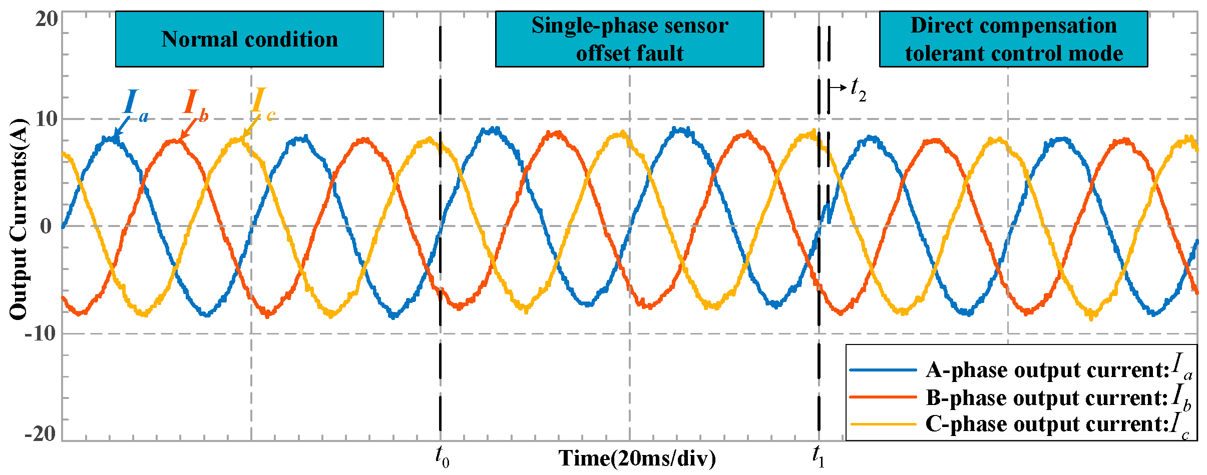
3.2.1. Direct Compensation Mode for Single-Phase Offset Fault

In (15), the average of offset fault feature D_ave can be obtained directly by the average current compensation mode. When a single-phase sensor offset fault occurs, D_ave can be expressed as:

$$D_{ave}=D_x/3,x=a,b,c$$

(20)

then the fault feature D_x can be calculated easily by D_ave:

$$D_x=3\times D_{ave}$$

(21)

Therefore, the compensation signal of direct compensation mode can be calculated:

$$R_{ave}=-3\times D_{ave}=-D_x$$

(22)

When the fault diagnosis result is a single-phase sensor offset fault, the direct compensation mode is chosen to add the compensation signal R_ave to the fault-phase sensed current.

$$I_{rx}=I_x+R_{ave}=i_x+D_x+R_{ave}=i_x$$

(23)

From (18), the sensed current returns back to the normal state through the direct compensation mode.

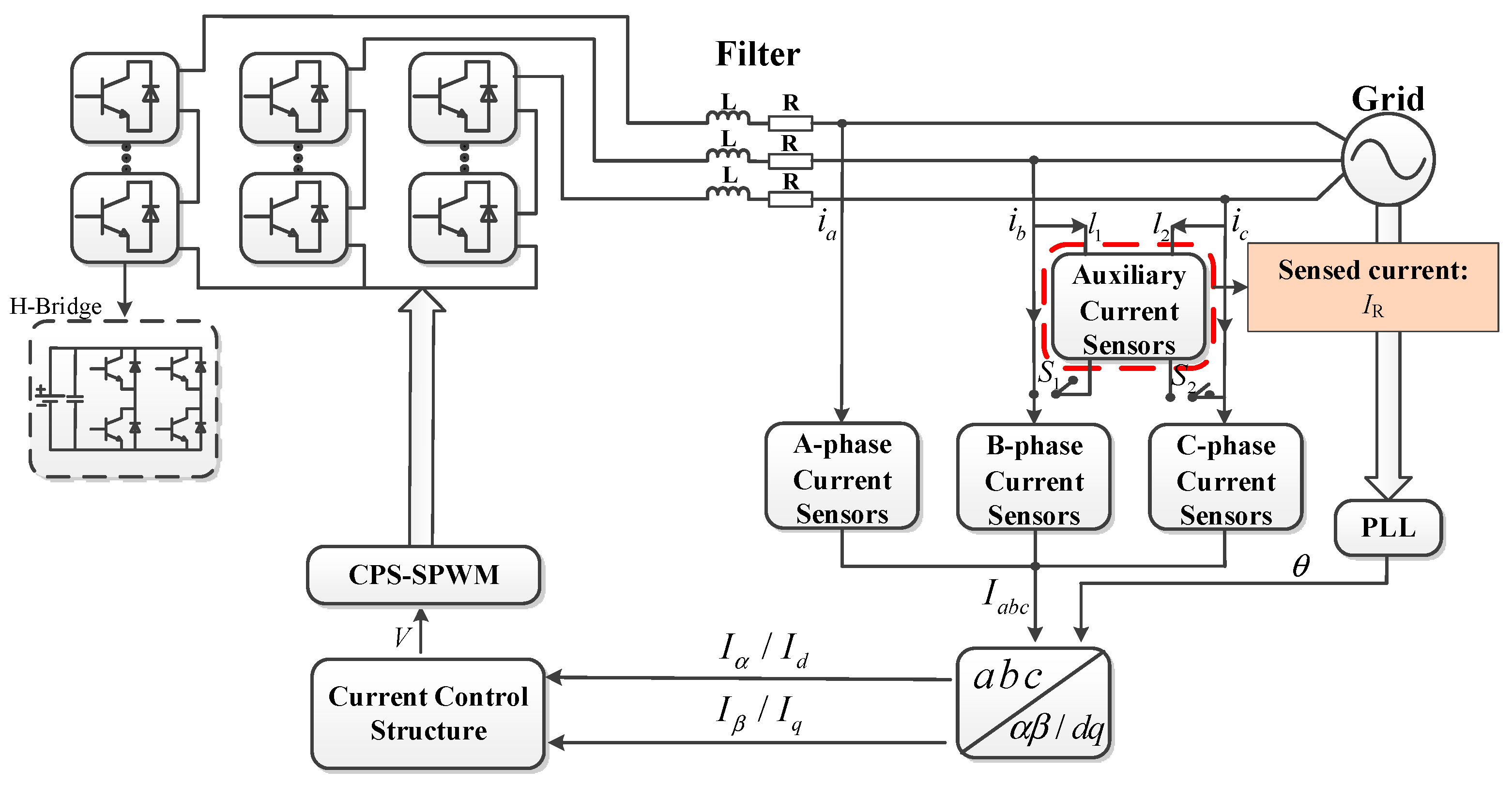
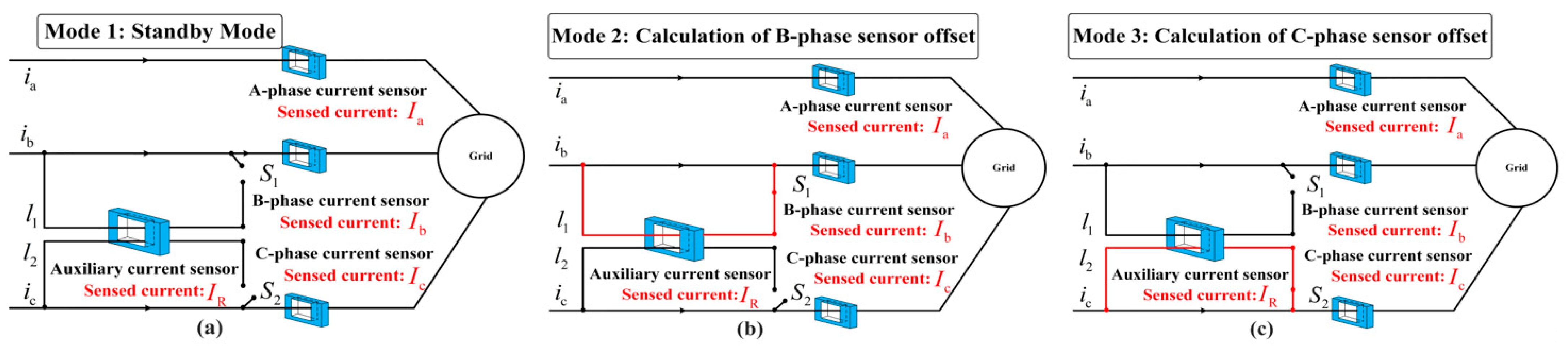
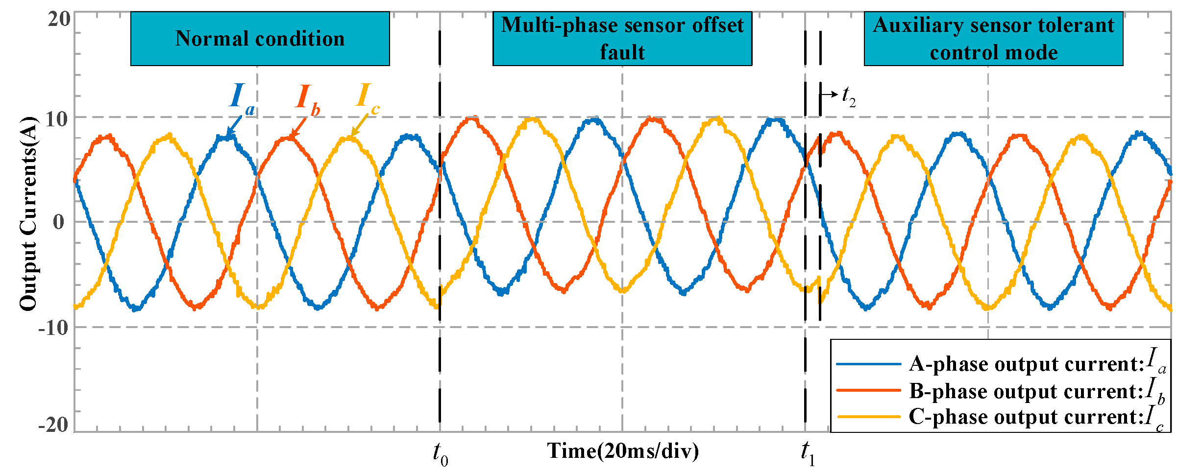
3.2.2. Indirect Compensation through An Auxiliary Current Sensor Mode for Multiphase Offset Fault

If the multiphase sensors simultaneously have an offset fault, the average of fault feature D_ave is represented as:

$$D_{ave}=(D_a+D_b+D_c)/3$$

(24)

The fault feature of each phase is different and cannot be determined only by D_ave. An auxiliary sensor mode is used as shown in Figure 4.

The auxiliary sensor mode structure includes an auxiliary sensor, two current bypasses (l₁, l₂), and two state change switches (S₁, S₂), as shown in Figure 4. In different states, the auxiliary sensor measures the current in different bypasses. Under normal conditions in Figure 5a, S₁, S₂ are disconnected, so the current passing through the auxiliary current sensor is zero. The auxiliary sensor is in standby mode under normal conditions, which makes the service life of the auxiliary sensor longer than the original current sensor in the system. Therefore, the auxiliary sensor can maintain high measurement accuracy even when the original sensors are faulty. In Figure 5b, under state 2, the bypass current in $l_1$ is measured, and the offset of the B-phase is calculated. In Figure 5c, under state 3, the bypass current in $l_2$ is measured, and the offset of the C-phase is calculated.

As is shown in Figure 5a, the original three current sensors in the system always measure three-phase currents. In the state transition process, the state change switches only change the current in the bypass, and the currents measured by the original three-phase sensors remain unchanged. Therefore, the state change of S₁, S₂ will not affect the performance of the original grid-connected system.

State 2 starts when the offset fault of B-phase current sensor occurs (Figure 5b). In this case, the auxiliary sensor is used to measure B-phase grid current i_b through a bypass. According to Kirchhoff’s current law, the sensed current of the B-phase sensor I_b and auxiliary sensor I_R can be expressed as follows:

$$\left\{\begin{array}{l}{I}_b=i_b+D_b\\ I_R=i_b/2\end{array}\right.$$

(25)

From (20), The fault component of the B-phase sensor D_b can be calculated as follows:

$$D_b=I_b-2I_R$$

(26)

Then, the state changes from 2 to 3 by state change switches (S₁, S₂) action. In state 3 (Figure 5c), the auxiliary sensor is used to measure the C-phase grid current i_c through a current bypass. The output current of the three-phase sensors and auxiliary sensor can be expressed as follows:

$$\left\{\begin{array}{l}{I}_R=i_c/2\\ I_a=i_a+D_a\\ I_b=i_b+D_b\\ I_c=i_c+D_c\end{array}\right.$$

(27)

In this case, the fault component of the C-phase sensor D_c can be calculate:

$$D_c=I_c-2I_R$$

(28)

In (21) and (23), D_b and D_c have been calculated. By substituting (21) and (23) into (19), the fault component of the C-phase sensor D_a can be calculated:

$$D_a=3\times D_{ave}-D_b-D_c$$

(29)

In state 3, the output current of the average current compensation mode is composed of normal current signals and fault features, that is

$$\left[\begin{array}{c}{I}_{c\alpha }\\ I_{c\beta }\end{array}\right]=\left[\begin{array}{c}2i_a/3-i_b/3-i_c/3+2D_a/3-D_b/3-D_c/3+D_{ave}\\ \sqrt{3}(i_b-i_c)/3+\sqrt{3}{D}_b/3-\sqrt{3}{D}_c/3+D_{ave}\end{array}\right]$$

(30)

The fault features D_a, D_b, and D_c have been calculated through the auxiliary sensor. D_ave is obtained by the average current compensation mode. Therefore, the compensation signal of auxiliary sensor tolerant control mode can be constructed as follows:

$$\left[\begin{array}{c}{R}_{\alpha }\\ R_{\beta }\end{array}\right]=\left[\begin{array}{c}-2D_a/3+D_b/3+D_c/3-D_{ave}\\ -\sqrt{3}{D}_b/3+\sqrt{3}{D}_c/-D_{ave}\end{array}\right]$$

(31)

When a multi-phase offset fault occurs, the compensation signals will be calculated by the auxiliary sensor mode, and it is added to the output of average current compensation mode:

$$\left[\begin{array}{c}{I}_{r\alpha }\\ I_{r\beta }\end{array}\right]=\left[\begin{array}{c}{I}_{c\alpha }+R_{\alpha }\\ I_{c\beta }+R_{\beta }\end{array}\right]=\left[\begin{array}{c}2i_a/3-i_b/3-i_c/3\\ \sqrt{3}(i_b-i_c)/3\end{array}\right]$$

(32)

From (27), there is no fault feature in the currents I_rα and I_rβ, which are the input signals of current control system, so the inverter can return to its normal condition.

The auxiliary sensor makes it possible to estimate the value of zero-offset in the case of simultaneous faults of multiple sensors. This paper also designs the switching circuit so that only an additional current sensor is needed.

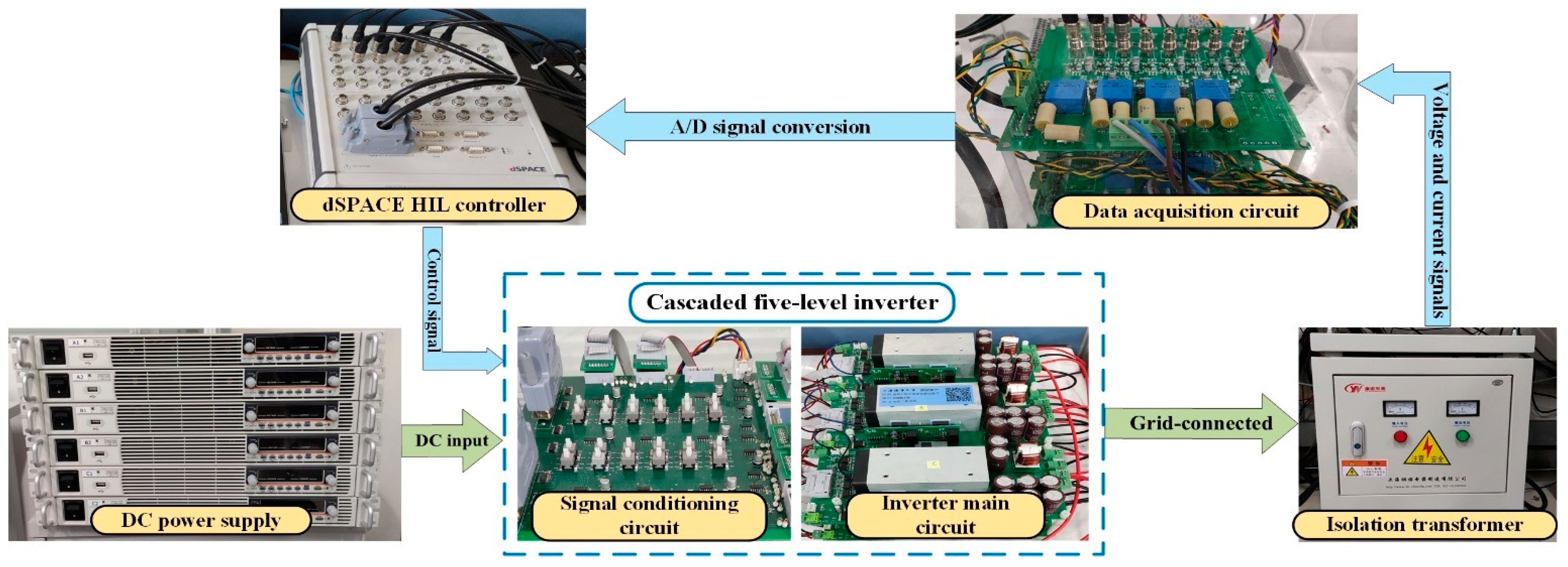
4. Experimental Result and Analysis

The proposed method is verified with a three-phase cascaded H-bridge five-level grid-connected inverter system. As shown in Figure 6, the experimental platform mainly includes a controller, data acquisition circuit, DC power supply, main circuit of the inverter, and an isolation transformer.

4.1. Data Acquisition under Various Failure Conditions

Table 1. System parameters.

System Parameters	Values
DC voltage	100 V
Filter inductance (L)	4 mH
Switching frequency	5 kHz
Grid voltage RMS	110 V
Grid frequency	50 Hz
Transformer ratio	1:2
Rated current RMS	5.656 A

gives the parameters of the system. The DC side is composed of six DC power supplies. The main circuit of the cascaded five-level inverter consists of six H-bridge units. The inverter’s main circuit is connected to the power grid through a filter circuit and an isolation transformer. The current control is implemented by the dSPACE HIL controller (DS1202).

4.2. Effectiveness of Fault Diagnosis

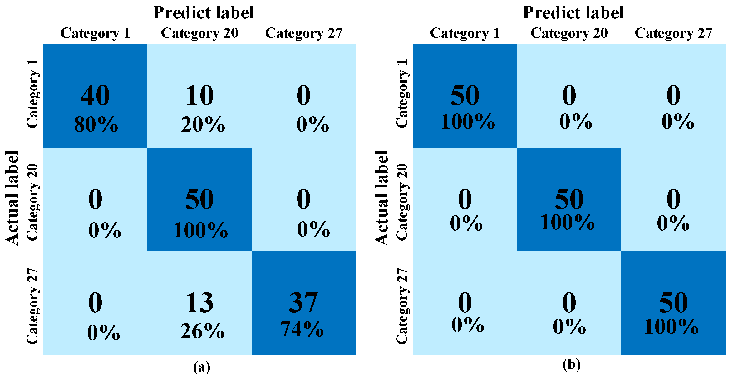
4.2.1. Average Current Compensation Mode

Figure 7 shows the steady state of A-phase grid voltage and A-phase output current using the average current compensation mode. It can be seen that from Figure 6, in the steady state, the peak value of the output current is 8 A which is equal to the reference value. The frequency of the output current is 50 Hz which is in phase with the grid voltage.

Figure 8 shows the dynamic response of the inverter with the average current compensation mode. In Figure 8a, the reference value of the d-axis current $I_d^{*}$ has a step change from 8 A to 10 A at t₀, the actual current I_d can track the change within 3 ms. The error between the d-axis reference current and d-axis actual current is shown in Figure 8b. In the state with reference current equal to 8 A, the error range can be kept within 0.4 A. When the step occurs, there is an obvious spike in the error, and the spike is eliminated quickly due to the current control system. In the state with reference current equal to 10 A, the error range can also be kept within 0.4 A. Figure 8c shows the waveforms of the output currents, it can be seen that the three-phase currents can quickly track the change in the reference value. Hence, the average current compensation mode will not affect the inverter dynamic performance.

4.2.2. Fault Diagnosis Results

A total of 27 types of three-phase current sensor offset faults are set in

Table 2. Three-phase current sensor fault types.

Fault Type	Specific Classification	Number
Healthy	Normal condition	1
Single-phase current sensor offset fault	positive offset 20%	3
	negative offset 10%	3
Two-phase current sensor offset fault	positive offset 20%	6
	negative offset 10%	6
Three-phase current sensor offset fault	positive offset 20%	4
	negative offset 10%	3

. Considering the offset fault, this is a random constant [24,25]. Therefore, to verify the generalization of the proposed method, the fault conditions of different offsets are set. Each phase current sensor is set with two offsets: a positive offset of 20% of the amplitude of the original signal and a negative offset of 10% of the amplitude of the original signal. Through the combination of three-phase fault conditions, 6 single-phase offset faults, 12 two-phase offset faults, and 8 three-phase offset faults can be set.

Collecting one cycle of three-phase output voltages as the diagnostic signals and collecting 100 samples for each fault situation, a total of 2700 samples are used for diagnosis. The data-based diagnosis method consists of three parts: data preprocessing, feature extraction, and fault classification [17]. According to [17], FFT (Fast Fourier Transform) and PCA (Principal Components Analysis) are used for data processing and feature extraction, respectively. For comparison, three classification algorithms are chosen, they are SVM (Support Vector Machine) [18], ELM (Extreme Learning Machine) [7], and BPNN (Back Propagation Neural Network) [26]. Randomly selecting 50 samples for training and 50 samples for testing under each fault condition, the diagnosis results of the test set are shown in the

Table 3. Comparison of diagnostic accuracy.

Control Structure	FFT + PCA + BP	FFT + PCA + BP	FFT + PCA + SVM
Traditional current control system	59.07%	93.60%	92.44%
Current control system with average current compensation mode	94.67%	99.06%	100%

. It can be seen that, under different diagnosis methods, the average current compensation mode can effectively improve the diagnosis accuracy. Among these methods, the best and most stable method is FFT + PCA + SVM, with an accuracy rate 100%.

As discussed in Section 2, when the offset values of three-phase sensors are identical, under traditional current control structure, the fault feature will disappear and lead to a reduced diagnostic accuracy. In order to verify this conclusion, the confusion matrices obtained by using FFT + PCA + SVM are compared in Figure 9.

Category 1, category 20, and category 27 in the figure represent the corresponding sensor fault conditions. According to Table 2, the 1st fault condition is the normal condition, the 20th fault condition is three-phase sensors having a 20% positive offset at same time, and the 27th fault condition is three-phase sensors having a 10% negative offset at same time. In Figure 9a, when the traditional current control structure is applied, 10 samples of 1st fault condition and 13 samples of 27th fault condition are incorrectly diagnosed as the 20th fault condition. Consistent with the simulation results, when the offsets of the three-phase sensor are the same, the fault characteristics will disappear and the diagnosis accuracy will be reduced under the traditional current control structure.

Figure 9b shows the diagnostic result under the proposed average current compensation mode. The fault feature of 20th and 27th fault conditions are reconstructed by the current average compensation signal. In this case, the 1st, 20th, and 27th fault conditions are well diagnosed. All the actual labels correspond well to the predicted labels, thus improving overall diagnostic accuracy.

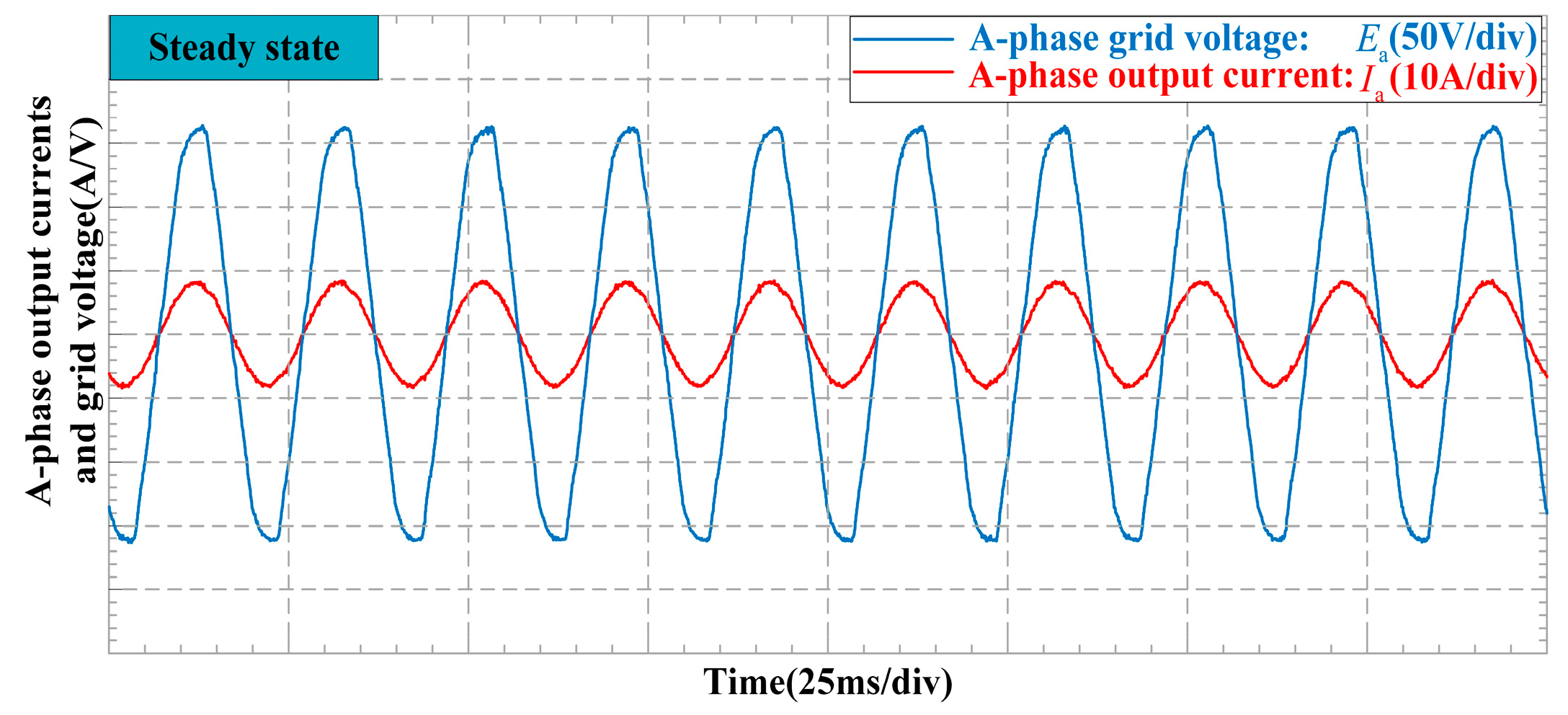
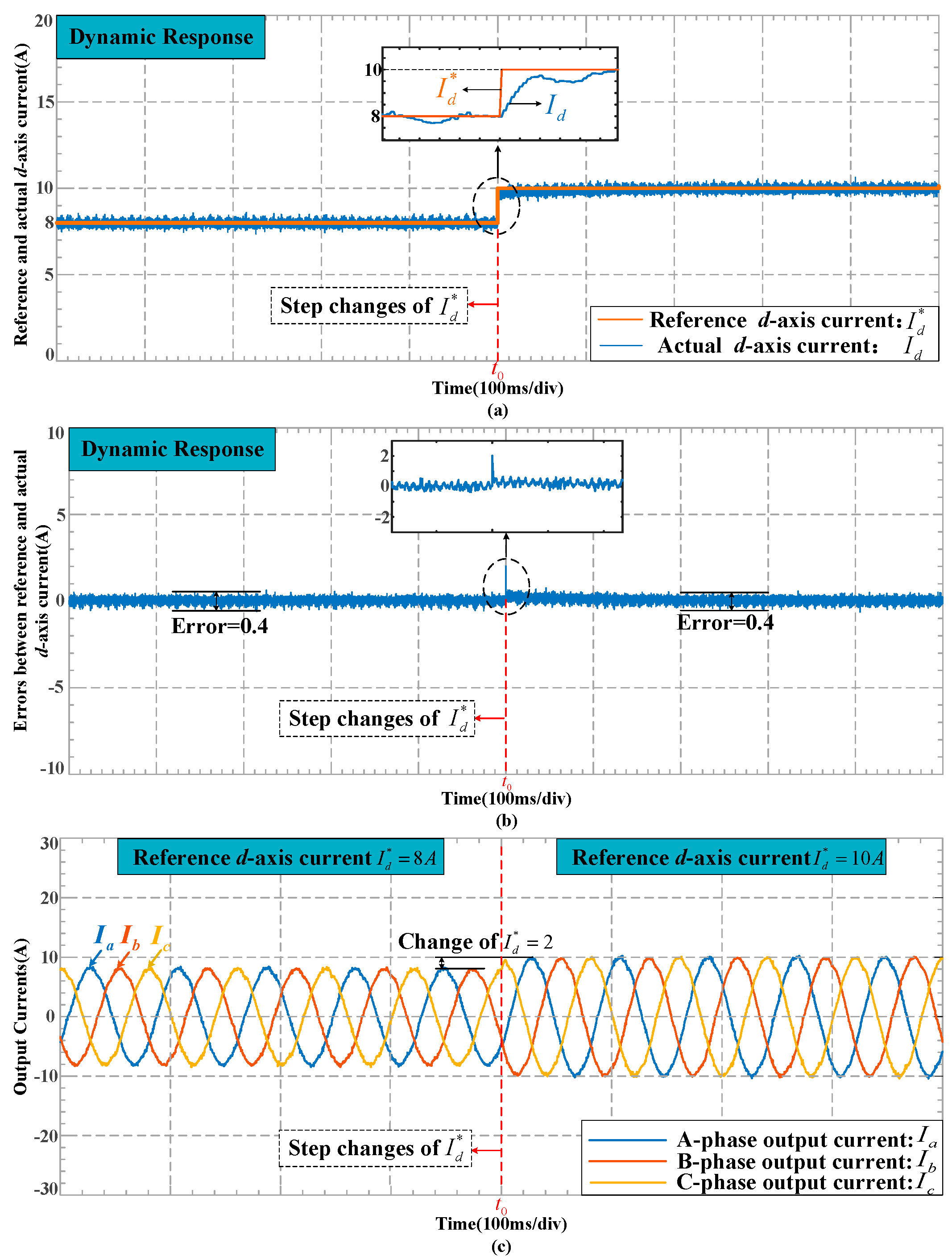
4.3. Performance of Multi-Mode Fault-Tolerant Control

4.3.1. Direct Compensation Mode for Single-Phase Offset Fault

Figure 10 shows the experimental results when the direct compensation mode is applied to the system. The A-phase sensor offset fault condition is set at t₀. Although only the A-phase sensor has an offset fault, the three-phase output currents are unbalanced due to the closed-loop control system. At t₁, the proposed tolerant control strategy of direct compensation mode is applied to the system. The corresponding fault offset can be calculated and compensated to the output current signal of the A-phase sensor. At t₂, the three-phase output currents can be restored to balance. Therefore, when a single-phase sensor offset fault occurs, the system can continue to operate normally for a short time.

4.3.2. Auxiliary Sensor Mode for Multiphase Offset Fault

The experimental result of auxiliary sensor mode is shown in Figure 11. At t₀, the three-phase sensors experience 20% offset faults. Compared with Figure 10, there is more obvious unbalanced change on the three-phase currents. The peak value of the normal output current is 8 A, and it reached 10 A under this fault condition. In this case, the auxiliary sensor tolerant control mode is applied to the system through the state change switch action. Between t₁ and t₂, the auxiliary sensor mode completes the state conversion and feeds back the compensation amount to the system. Then, the three-phase output currents return back to the normal state within 2 ms. Therefore, the proposed fault-tolerant control method of the auxiliary sensor model can make the three-phase output current quickly recover to normal condition. In addition, since the state switch of the auxiliary sensor model only changes the current in the current bypass, the fault-tolerant control method does not affect the original system performance.

Table 4. Comparison of fault-tolerant control strategy.

Fault-Tolerant Control Strategy	Number of Fault Sensors	Tolerance Time	Whether It Improves the Diagnosis Accuracy
Proposed strategy	Multiple	2 ms	Yes
Independent observer [14]	Single or double	8 ms	No
Signal reconstruction [16]	Single	40 ms	No
Vector space decomposition [13]	Multiple	10 ms	No
Signal compensator [15]	Single or double	4 s	No

lists the different performance indicators of the proposed strategy and the existing fault-tolerant control strategy introduced in Section 1.

Compared with independent observer, signal reconstruction, and signal compensator, it can be seen that the proposed strategy is suitable for the simultaneous fault of multiple sensors. Additionally, the proposed strategy has shorter fault tolerance time than the other four methods. In addition, the proposed strategy can effectively improve the diagnosis accuracy which is a prominent feature of the proposed strategy.

5. Conclusions

In the case of multiple current sensor faults, the closed-loop control system will affect the fault characteristics. This paper proposes a multi-mode fault-tolerant control method. The proposed strategy is composed of the average current compensation mode, fault diagnostic, and multi-mode fault-tolerant control. For the average current compensation mode, the current average signal is calculated and compensated to the frame transformation process; it does not affect the stability of the original system due to Kirchhoff’s current law. Under sensor fault conditions, the fault features are reconstructed, and the compensation signal improves the features discrimination. The diagnostic accuracy has been effectively improved due to the reconstructed features. After the fault location is accurately determined, the multi-mode fault-tolerant control method is activated. In the case of a single sensor fault, the system adopts direct compensation mode without hardware redundancy. A new auxiliary sensor mode is proposed for multiple sensor faults. Only an additional current sensor is needed to estimate the offsets of the three-phase current sensors. The proposed strategy can quickly restore the system from various fault states to the normal states according to the experimental results.

References

1. Cai, B.; Zhao, Y.; Liu, H.; Xie, M. A Data-Driven Fault Diagnosis Methodology in Three-Phase Inverters for PMSM Drive Systems. IEEE Trans. Power Electron. 2017, 32, 5590–5600. [Google Scholar] [CrossRef]
2. Anand, A.; Raj, N.; Jagadanand, G.; George, S. A Generalized Switch Fault Diagnosis for Cascaded H-Bridge Multilevel Inverters Using Mean Voltage Prediction. IEEE Trans. Ind. Appl. 2020, 56, 1563–1574. [Google Scholar] [CrossRef]
3. Bae, C.J.; Lee, D.C.; Nguyen, T.H. Detection and identification of multiple IGBT open-circuit faults in PWM inverters for AC machine drives. IET Power Electron. 2020, 12, 923–931. [Google Scholar] [CrossRef]
4. Kim, W.J.; Kim, S.H. ANN design of multiple open-switch fault diagnosis for three-phase PWM converters. IET Power Electron. 2020, 19, 4490–4497. [Google Scholar] [CrossRef]
5. Mtepele, K.O.; Campos-Delgado, D.U.; Valdez-Fernández, A.A.; Pecina-Sánchez, J.A. Model-based strategy for open-circuit faults diagnosis in n-level CHB multilevel converters. IET Power Electron. 2019, 12, 648–655. [Google Scholar] [CrossRef]
6. Yao, G.; Li, Y.; Li, Q.; Hu, S.; Jin, N. Model predictive power control for a fault-tolerant grid-connected converter using reconstructed currents. IET Power Electron. 2020, 13, 1181–1190. [Google Scholar] [CrossRef]
7. Li, Z.; Wheeler, P.; Watson, A.; Costabeber, A.; Wang, B.; Ren, Y.; Bai, Z.; Ma, H. A Fast Diagnosis Method for Both IGBT Faults and Current Sensor Faults in Grid-Tied Three-Phase Inverters with Two Current Sensors. IEEE Trans. Power Electron. 2020, 35, 5267–5278. [Google Scholar] [CrossRef]
8. Rajendran, S.; Govindarajan, U.; Senthilvadivelu, S.; Uandai, S.B. Intelligent sensor fault-tolerant control for variable speed wind electrical systems. IET Power Electron. 2013, 6, 1308–1319. [Google Scholar] [CrossRef]
9. Xia, J.; Guo, Y.; Dai, B.; Zhang, X. Sensor Fault Diagnosis and System Reconfiguration Approach for an Electric Traction PWM Rectifier Based on Sliding Mode Observer. IEEE Trans. Ind. Appl. 2017, 53, 4768–4778. [Google Scholar] [CrossRef]
10. Chakraborty, C.; Verma, V. Speed and Current Sensor Fault Detection and Isolation Technique for Induction Motor Drive Using Axes Transformation. IEEE Trans. Ind. Electron. 2015, 62, 1943–1954. [Google Scholar] [CrossRef]
11. Gou, B.; Xu, Y.; Xia, Y.; Deng, Q.; Ge, X. An Online Data-Driven Method for Simultaneous Diagnosis of IGBT and Current Sensor Fault of Three-Phase PWM Inverter in Induction Motor Drives. IEEE Trans. Power Electron. 2020, 35, 13281–13294. [Google Scholar] [CrossRef]
12. Huang, Z.; Wang, Z.; Zhang, H. A Diagnosis Algorithm for Multiple Open-Circuited Faults of Microgrid Inverters Based on Main Fault Component Analysis. IEEE Trans. Energy Convers. 2018, 33, 925–937. [Google Scholar] [CrossRef]
13. Kou, L.; Liu, C.; Cai, G.; Zhou, J.; Yuan, Q.; Pang, S. Fault diagnosis for open-circuit faults in NPC inverter based on knowledge-driven and data-driven approaches. IET Power Electron. 2020, 13, 1236–1245. [Google Scholar] [CrossRef]
14. Wang, T.; Xu, H.; Han, J.; Elbouchikhi, E.; Benbouzid, M.E.H. Cascaded H-Bridge Multilevel Inverter System Fault Diagnosis Using a PCA and Multiclass Relevance Vector Machine Approach. IEEE Trans. Power Electron. 2015, 30, 7006–7018. [Google Scholar] [CrossRef]
15. Xia, Y.; Xu, Y.; Gou, B. A Data-Driven Method for IGBT Open-Circuit Fault Diagnosis Based on Hybrid Ensemble Learning and Sliding-Window Classification. IEEE Trans. Ind. Inform. 2020, 16, 5223–5233. [Google Scholar] [CrossRef]
16. Jiang, Q.; Yan, X.; Huang, B. Performance-Driven Distributed PCA Process Monitoring Based on Fault-Relevant Variable Selection and Bayesian Inference. IEEE Trans. Ind. Electron. 2016, 63, 377–386. [Google Scholar] [CrossRef]
17. Wang, Y.; Ma, X.; Qian, P. Wind Turbine Fault Detection and Identification Through PCA-Based Optimal Variable Selection. IEEE Trans. Sustain. Energy 2018, 9, 1627–1635. [Google Scholar] [CrossRef] [Green Version]
18. Zhong, K.; Han, M.; Qiu, T.; Han, B.; Chen, Y.W. Distributed Dynamic Process Monitoring Based on Minimal Redundancy Maximal Relevance Variable Selection and Bayesian Inference. IEEE Trans. Control. Syst. Technol. 2020, 28, 2037–2044. [Google Scholar] [CrossRef]
19. Wang, X.; Wang, Z.; Xu, Z.; Cheng, M.; Wang, W.; Hu, Y. Comprehensive Diagnosis and Tolerance Strategies for Electrical Faults and Sensor Faults in Dual Three-Phase PMSM Drives. IEEE Trans. Power Electron. 2019, 34, 6669–6684. [Google Scholar] [CrossRef]
20. Yu, Y.; Zhao, Y.; Wang, B.; Huang, X.; Xu, D. Current Sensor Fault Diagnosis and Tolerant Control for VSI-Based Induction Motor Drives. IEEE Trans. Power Electron. 2018, 33, 4238–4248. [Google Scholar] [CrossRef]
21. Salmasi, F.R. A Self-Healing Induction Motor Drive with Model Free Sensor Tampering and Sensor Fault Detection, Isolation, and Compensation. IEEE Trans. Ind. Electron. 2017, 64, 6105–6115. [Google Scholar] [CrossRef]
22. Gou, B.; Ge, X.; Liu, Y.; Feng, X. Load-current-based current sensor fault diagnosis and tolerant control scheme for traction inverters. Electron. Lett. 2016, 52, 1717–1719. [Google Scholar] [CrossRef]
23. Wang, T.; Qi, J.; Xu, H.; Wang, Y.; Liu, L.; Gao, D. Fault diagnosis method based on FFT-RPCA-SVM for Cascaded-Multilevel Inverter. ISA Trans. 2016, 60, 156–163. [Google Scholar] [CrossRef]
24. 519-2014; IEEE Recommended Practice and Requirements for Harmonic Control in Electric Power Systems. (Revision of IEEE Std 519-1992). Institute of Electrical and Electronics Engineers, Inc.: Piscataway, NJ, USA, 2014; pp. 1–29.
25. Yu, Y.; Hu, X. Active Disturbance Rejection Control Strategy for Grid-Connected Photovoltaic Inverter Based on Virtual Synchronous Generator. IEEE Access 2019, 7, 17328–17336. [Google Scholar] [CrossRef]
26. Kumar, N.; Saha, T.K.; Dey, J. Sliding-Mode Control of PWM Dual Inverter-Based Grid-Connected PV System: Modeling and Performance Analysis. IEEE J. Emerg. Sel. Top. Power Electron. 2016, 4, 435–444. [Google Scholar] [CrossRef]
27. Merabet, A.; Labib, L.; Ghias, A.M.Y.M.; Ghenai, C.; Salameh, T. Robust Feedback Linearizing Control with Sliding Mode Compensation for a Grid-Connected Photovoltaic Inverter System Under Unbalanced Grid Voltages. IEEE J. Photovolt. 2017, 7, 828–838. [Google Scholar] [CrossRef]
28. Zmood, D.; Holmes, D. Stationary frame current regulation of PWM inverters with zero steady state error. IEEE Trans. Power Electron. 2003, 18, 814–822. [Google Scholar] [CrossRef]
29. Timbus, A.; Liserre, M.; Teodorescu, R.; Rodriguez, P.; Blaabjerg, F. Evaluation of Current Controllers for Distributed Power Generation Systems. IEEE Trans. Power Electron. 2009, 24, 654–664. [Google Scholar] [CrossRef]
30. Gou, B.; Xu, Y.; Xia, Y.; Wilson, G.; Liu, S. An Intelligent Time-Adaptive Data-Driven Method for Sensor Fault Diagnosis in Induction Motor Drive System. IEEE Trans. Ind. Electron. 2019, 66, 9817–9827. [Google Scholar] [CrossRef]
31. Balaban, E.; Saxena, A.; Bansal, P.; Goebel, K.F.; Curran, S. Modeling, Detection, and Disambiguation of Sensor Faults for Aerospace Applications. IEEE Sens. J. 2009, 9, 1907–1917. [Google Scholar] [CrossRef]
32. Zhang, Z.; Xiao, B. Sensor Fault Diagnosis and Fault Tolerant Control for Forklift Based on Sliding Mode Theory. IEEE Access 2020, 8, 84858–84866. [Google Scholar] [CrossRef]
Figure 1. Block diagram of cascaded H-bridge grid-connected inverter.
Machines 11 00061 g001
Figure 2. A−phase sensed current under offset fault condition.
Machines 11 00061 g002
Figure 3. Block diagram of fault-tolerant control strategy based on average current compensation.
Machines 11 00061 g003
Figure 4. Physical circuit diagram containing the auxiliary sensor.
Machines 11 00061 g004
Figure 5. Operating modes of the auxiliary current sensor. (a) Mode 1: Normal condition. (b) Mode 2: Calculation of B-phase sensor zero-offsets. (c) Mode 3: Calculation of C-phase sensor zero-offsets.
Machines 11 00061 g005
Figure 6. Grid-connected inverter experimental platform.
Machines 11 00061 g006
Figure 7. A-phase grid voltage and A-phase output current.
Machines 11 00061 g007
Figure 8. System dynamic response. (a) D−axis reference current and actual current (b) Error between d−axis reference current and actual current (c) Three phase output current.
Machines 11 00061 g008
Figure 9. Confusion matrices obtained by FFT + PCA + SVM. (a) The results applied to traditional current control structure. (b) The results applied to the average current compensation mode.
Machines 11 00061 g009
Figure 10. Experimental results for single−phase sensor offset fault using direct compensation tolerant control mode.
Machines 11 00061 g010
Figure 11. Experimental results for multi−phase sensor offset fault using auxiliary sensor tolerant control mode.
Machines 11 00061 g011