Common Noninteracting Control with Simultaneous Common Partial Zeroing with Application to a Tracked UGV ^†

Abstract

In several MIMO system applications, the deviations of some output performance variables from their nominal values are required to be controlled independently, while the other performance variables are required to remain at their nominal value. This problem, named noninteracting control with simultaneous partial output zeroing, is important in the case of the common design of multi-model systems. To this end, the problem of a common noninteracting control with simultaneous common partial output zeroing is formulated. The present paper aims to develop a solution to the problem of multi-model normal linear time-invariant systems via regular and static measurement output feedback. The present approach follows the method developed for the solution of the common I/O decoupling problem. The main results of the paper are the introduction and the formulation of the problem at hand, the establishment of the necessary and sufficient conditions for its solvability, and the derivation of the respective general solution of the controller matrices. For the resulting closed-loop system, the additional design requirement of approximate command following a simultaneous I/O stabilizability is studied using a composite norm 2 type cost function and a metaheuristic algorithm for the derivation of the free parameters of the controller. The present results are illustrated through a numerical example of a nonlinear process with two operating points. Moreover, all the above results are successfully applied to the two-model description of a robot-tracked UGV, using a common controller feeding back measurements of the motor currents and the orientation of the vehicle.

1. Introduction

The present paper introduces a new design requirement in the family of noninteracting control problems. The design requirement is that of a common noninteracting control with simultaneous common partial output zeroing for multi-model linear time-invariant systems. The special case of the present design requirement, where the number of system inputs is greater than or equal to the number of system outputs, was presented in [1].

The present design requirement belongs to the class of common design problems. The common control design is an indispensable step that should be checked before proceeding to switching. The common control design has a long history (see [2,3,4,5,6,7,8,9,10,11]) and several applications; indicatively, see [9,10,11], where the case of robot manipulators was studied. In the framework of the present common design requirement, studied for the class of multi-model normal linear time-invariant systems, the set of the outputs of each model of the multi-model system is divided into two subsets. Each output belonging to the first subset is required to be controlled independently by a respective external command. The rest outputs, namely the outputs belonging to the second subset, are required to be equal to zero, independently from the choice of the external commands. It is important to point out that the partition of the set of the system outputs into two subsets depends upon the respective model of the multi-model description. So, the two subsets may be different for different models of the multi-model system description. After an appropriate row rearrangement, the transfer matrices of the closed-loop systems, resulting after the application of the common controller, are expressed in four block forms. One block form is a rational diagonal matrix, and the remaining three are zero blocks. The main motivation for the derivation of the results of the present paper was the observation that, in several MIMO system applications, the deviations of some output performance variables from their nominal values are required to be controlled independently, while the other performance variables are required to remain at their nominal value.

Here, the design requirement of common noninteracting control with simultaneous common partial output zeroing is solved using a regular static measurement output controller. The solvability conditions of this design problem are established, and the general solution of the common controllers, solving the problem, is determined. Additionally, the design requirement of the approximate asymptotic command following is studied by the appropriate choice of the free parameters of the precompensator matrix. The remaining free parameters of the common controller are derived using a metaheuristic algorithm (see [12,13]) that is executed towards the minimization of a 2-norm cost, evaluating the performance of the transient responses of the closed-loop systems. Finally, the results of the proposed common design scheme are illustrated through a numerical example, where a nonlinear process in two different operating points is controlled. It is mentioned that the pure (noncommon) output zeroing problem, presented in [14], requires the deviations of the system outputs from their nominal values to be equal to zero, i.e., the original performance variables are required to remain at their desired operating values.

Before closing the presentation of the design results of the present paper, it is important to mention that the design requirement of a common noninteracting control with simultaneous common partial output zeroing was studied in [1] for the special case where the number of inputs is greater than or equal to the number of outputs. Finally, it is mentioned that in [1], a rather abstractive presentation of the design procedure and the proofs of the results was presented. Here, the complete design procedure, using all the required formalism, is presented.

Another motivation for the derivation of the present design results is the open control problem of the two-model robot-tracked vehicle description presented in [15,16]. Tracked Unmanned Ground Vehicles (UGVs) are important for open land applications, where conventional robotic vehicles or two-legged robots are not appropriate. Indicative applications (see [15,16,17,18,19,20,21,22]) are met in agriculture, surveillance, patrols, the transfer of goods, emergency situations, the military, underwater operations, and constructions. It is important to mention that the control problem of the two-model robot-tracked vehicle description in [15,16] has not yet been studied.

The precision and accuracy of the operations of Tracked UGVs depend greatly upon control efficiency. Several approaches and models were proposed (indicatively, see [15,16,22,23,24,25,26,27,28,29,30,31,32,33]) to handle the issue. In [15,16], a two-model variable switching description of a robot-tracked vehicle was proposed. The models include the simplified dynamics of the rigid body and the motors driving the vehicle. The switching condition between the models is in the form of a sharp constraint upon the forces that are generated to be the left-side and right-side motors. In [22], the mathematical description of an unmanned tracked excavator vehicle that is equipped with an excavation arm was developed. In [23], a switching dynamic description of a tracked vehicle was presented, and a speed-regulating control strategy and a torque-regulating control strategy were developed. In [24], the mathematical description of a tracked vehicle was presented in modular form, and a Stanley-type controller was derived. In [25], the mathematical description model of a 3DOF-tracked mobile robot, including the dynamics and kinematics of the skid-steering mechanism, was presented, and a PID controller was applied to control the speed of the vehicle. In [26], based on the kinematics of a robot-tracked vehicle, a control law for trajectory tracking under slip conditions, system constraints, and varying dynamics were presented. In [27], the problem of localization and trajectory tracking control under slip conditions was investigated based on the kinematics of a robot-tracked vehicle. The approach was based on feedback linearization and indirect Kalman filtering. In [28], the dynamic system description of a tracked vehicle undergoing skid-steering on horizontal hard terrain was presented. The vehicle’s path was controlled via a modified PID computed torque control scheme. In [29,30], the problem of trajectory tracking control of an autonomous tracked vehicle was investigated through a backstepping kinematic controller and an integral sliding mode controller based on vehicle dynamics. In [31], the problem of position control for a tracked vehicle was studied using driving force control and virtual-turning velocity control. In [32], the problem of the steering control of tracked vehicles was studied through differential steering control rules and a Fuzzy PID control scheme. In [33], three control strategies were proposed for the investigation of the closed-loop dynamical performance of tracked vehicles using different desired trajectories. The three control schemes were a robust nonlinear controller, a speed compensation-based fuzzy logic controller, and a speed compensation-based proportional–integral controller.

In the present paper, based on the two-model description of the Tracked UGV presented in [15,16] and the herein-derived theoretical results, the independent forward and angular motion of the robot vehicle is achieved for the case where the performance outputs are the linear velocity and the heading angle. Here, the measurement variables are the two motor currents and the heading angle of the vehicle. These measurements are clearly offered for acquisition by a small-scale embedded controller. The problem of common noninteracting control with partial output zeroing is proven to be solvable, and the controller matrices’ general solution is derived. This general solution achieves approximate command following and I/O stability using the previously mentioned metaheuristic algorithm. The present application was studied in [1]. Furthermore, in the case where the four mechanical resistances of the vehicle, as well as the lateral friction of the tracks, are uncertain, it is shown through extensive simulation experiments that the efficiency of the derived common controller remains satisfactory. This result provides promising perspectives for physical experimentation using the derived controller. Finally, the performance of the derived common controller for the Tracked UGV is compared to a switching controller designed to satisfy noninteracting control with simultaneous partial output zeroing for each model of the Tracked UGV. The superiority of the performance of the common controller is illustrated through the simulation results for a composite maneuver.

2. Noninteracting Control with Simultaneous Partial Output Zeroing for Single Model Descriptions

2.1. Definition of the Design Requirement

Consider the linear time-invariant system description:

$$\dot{x}(t)=Ax(t)+Bu(t),x_0=x(0-) , y(t)=Cx(t), y_M(t)=C_{M}x(t) ,$$

(1)

where $x(t)\in {ℝ}^n$ is the state vector, $u(t)\in {ℝ}^m$ is the control input vector, $y(t)\in {ℝ}^p$ is the performance output vector, and $y_M(t)\in {ℝ}^{p_M}$ is the measurement output vector. The parameters $n$, $m$ and $p$ are positive integers. The parameter $p_M$ is a nonnegative integer. The parameters $m$ and $p$ are greater than or equal to 2.

The controller is of the static measurement output form

$$u(t)=F_M{y}_M(j,t)+Gw(t),$$

(2)

where $w(t)\in {ℝ}^{m_E}$ is the vector of external commands, the parameter $m_E$ is a natural number, being greater than or equal to 2, $F_M\in {ℝ}^{m\times p_M}$ is the feedback matrix, and $G\in {ℝ}^{m\times m_E}$ is the precompensator matrix.

The design requirement is the following: each performance output, in a predefined set of performance outputs, is independently controlled by a respective external command, while the rest of the outputs are equal to zero. In this design requirement, we refer to the forced response of the system.

The performance output vector is expressed with respect to its elements as $y={\left[\begin{array}{ccc}{y}_1& \cdots & y_p\end{array}\right]}^T$. Let ${\mathbb{S}}_I\subseteq \{y_1,\dots ,y_p\}$ be a predefined set of output variables. The set of the rest of the outputs is defined to be ${\mathbb{S}}_O=\{y_1,\dots ,y_p\}-{\mathbb{S}}_I$. Let $p_I=\mathrm{card}\left({\mathbb{S}}_I\right)$ and $p_O=\mathrm{card}\left({\mathbb{S}}_O\right)$, where $\mathrm{card}\left(·\right)$ denotes the cardinality of the argument set. Clearly, it holds that $p_I+p_O=p$.

Let

$$J=\left[\begin{array}{c}{J}_I\\ J_O\end{array}\right]; J\in {ℝ}^{p\times p}, J_I\in {ℝ}^{p_I\times p}, J_O\in {ℝ}^{p_O\times p},$$

(3)

be a row rearrangement matrix, setting first the elements of $y={\left[\begin{array}{ccc}{y}_1& \cdots & y_p\end{array}\right]}^T$ belonging to ${\mathbb{S}}_I$, i.e., the elements of $y$ are rearranged, and the rearranged vector has the form

$$y_J=Jy=\left[\begin{array}{c}{J}_{I}y\\ J_{O}y\end{array}\right]$$

The rows of the output matrix are rearranged accordingly, i.e.,

$$C_J=\left[\begin{array}{c}{C}_I\\ C_O\end{array}\right]=JC=\left[\begin{array}{c}{J}_{I}C\\ J_{O}C\end{array}\right].$$

(4)

The design requirement is expressed, using the above definitions, as follows: the forced responses of the first $p_I$ elements of $y_J$ are decoupled; namely, they are controlled independently by respective external commands, while the forced responses of the rest elements of $y_J$ are required to be equal to zero, independently of the external commands. The latter expression of the design requirement is formally stated as follows: find the appropriate $F_M$, $G$ and $h_i(s)$, where $i\in \{1,\dots ,p_I\}$, such that the following equation is satisfied:

$$\left[\begin{array}{c}{C}_I\\ C_O\end{array}\right]{\left(s{I}_n-A-B{F}_M{C}_M\right)}^{-1}BG=\left[\begin{array}{cc}\underset{i=1,\dots ,p_I}{\mathrm{diag}}\left\{h_i(s)\right\}& 0_{p_I\times (m_E-p_I)}\\ 0_{p_O\times p_I}& 0_{p_O\times (m_E-p_I)}\end{array}\right],$$

(5)

where $h_i(s)$ are different than the zero rational functions of $s$ with real coefficients, i.e.,

$$h_i(s)\in ℝ(s)-\left\{0\right\}, \forall i\in \{1,\dots ,p_I\}.$$

(6)

where $ℝ(s)$ is the field rational functions of $s$ with real coefficients.

2.2. Interpretation and Characteristics of the Design Requirement

A linear description of the form (1) is usually met as the linear approximant of a nonlinear process description around an operating point. It is plausible to require some of the performance output variables of the original nonlinear model to move independently to new operating values while the rest are required to remain at their respective operating values. In terms of the linear approximant, this design goal is clearly translated to the requirement (5). The above interpretation is also valuable in the case of the nonlinear models of composite robotic systems studied through linear approximants around nominal operating points.

Regarding the formal definition of the problem in (5), it is important to mention that there are two cases of particular importance. The first is the case $m_E=p_I$. The second is the case of

$$m_E=\mathrm{rank}B,$$

(7)

$$p_I\le \mathrm{rank}B, p_I\ge 1,$$

(8)

The natural number $p$ can have any relative value with respect to $\mathrm{rank}B$. The second case is the case that will be studied here. Without loss of generality, it can be considered that the matrix $B$ is of full column rank and that the number of states is greater than or equal to the number of control inputs, i.e.,

$$\mathrm{rank}B=m, n\ge m.$$

(9)

Regarding the second case, it is important to mention that if the system description is a single model description and all performance outputs of (1), namely, all elements of ${\mathbb{S}}_I\cup {\mathbb{S}}_O$, can be independently controlled by the respective external commands of the controller, i.e., the system in (1) is fully decouplable, the problem formulated in (5) would be of limited interest. In the multi-model case with a common controller, which will be studied in the following section, the problem is of significant importance since, in multi-model closed-loop descriptions, different external commands may be required to be different from zero for different models of the multi-model description. To illustrate this remark, consider the following example of a three-model system, where the desired closed-loop transfer matrices of the 1st, the 2nd, and the 3rd model, respectively, are the following:

$$\left[\begin{array}{ccccc}{h}_1(1,s)& 0& 0& 0& 0\\ 0& h_2(1,s)& 0& 0& 0\\ 0& 0& h_3(1,s)& 0& 0\\ 0& 0& 0& h_4(1,s)& 0\\ 0& 0& 0& 0& 0\end{array}\right],$$

$$\left[\begin{array}{ccccc}{h}_1(2,s)& 0& 0& 0& 0\\ 0& 0& 0& 0& 0\\ 0& 0& 0& 0& 0\\ 0& 0& 0& h_4(2,s)& 0\\ 0& 0& 0& 0& 0\end{array}\right],$$

$$\left[\begin{array}{ccccc}{h}_1(3,s)& 0& 0& 0& 0\\ 0& h_2(3,s)& 0& 0& 0\\ 0& 0& h_3(3,s)& 0& 0\\ 0& 0& 0& 0& 0\\ 0& 0& 0& 0& 0\end{array}\right].$$

For the present three model description, the respective output matrices are

$$\left[\begin{array}{c}{C}_I(1)\\ C_O(1)\end{array}\right]=\left[\begin{array}{cc}{I}_4& 0\\ 0& I_1\end{array}\right]C(1),$$

$$\left[\begin{array}{c}{C}_I(2)\\ C_O(2)\end{array}\right]=\left[\begin{array}{ccccc}1& 0& 0& 0& 0\\ 0& 0& 0& 1& 0\\ 0& 1& 0& 0& 0\\ 0& 0& 1& 0& 0\\ 0& 0& 0& 0& 1\end{array}\right]C(2),$$

$$\left[\begin{array}{c}{C}_I(3)\\ C_O(3)\end{array}\right]=\left[\begin{array}{cc}{I}_3& 0\\ 0& I_2\end{array}\right]C(3).$$

The first argument of the above rational functions and the single argument of the above matrices is the number of the model. In the following section, the problem at hand for multi-model descriptions will be studied using common controllers.

3. Common Noninteracting Control with Simultaneous Common Partial Output Zeroing for Multi-Model Descriptions

3.1. Definition of the Common Design Requirement

Consider the multi-model linear time-invariant system description (see also [1,9,10])

$$\dot{x}(j,t)=A(j)x(j,t)+B(j)u(t), x_{0,j}=x(j,0-),$$

(10a)

$$y(t)=C(j)x(j,t), y_M(t)=C_M(j)x(j,t) ;j\in \{1,\dots ,N\},$$

(10b)

where $x(j,t)\in {ℝ}^n$ is the state vector, $u(t)\in {ℝ}^m$ is the control input vector, $y(t)\in {ℝ}^p$ is the performance output vector, and $y_M(j,t)\in {ℝ}^{p_M}$ is the measurement output vector. The parameters $n, m$, $p$, and $p_M$ were already presented in the previous section. Moreover, similarly to the previous section and without a loss of generality, the following assumptions are considered:

$$\mathrm{rank}B(j)=m, \forall j\in \{1,\dots ,N\}, n\ge m.$$

(11)

In the present multi-model case, the outputs are also grouped into two sets, depending upon the index of the respective model. Let ${\mathbb{S}}_I(j)\subseteq \{y_1,\dots ,y_p\}$ be the predefined set of outputs. The set of the rest of the outputs is defined to be ${\mathbb{S}}_O(j)=\{y_1,\dots ,y_p\}-{\mathbb{S}}_I(j)$. Let $p_I(j)=\mathrm{card}\left({\mathbb{S}}_I(j)\right)$ and $p_O(j)=\mathrm{card}\left({\mathbb{S}}_O(j)\right)$. Clearly, it holds that

$$p_I(j)+p_O(j)=p, \forall j\in \{1,\dots ,N\}.$$

(12)

Let

$$J(j)=\left[\begin{array}{c}{J}_I(j)\\ J_O(j)\end{array}\right]; J(j)\in {ℝ}^{p\times p}, J_I(j)\in {ℝ}^{p_I(j)\times p}, J_O(j)\in {ℝ}^{p_O(j)\times p},$$

(13)

be a row rearrangement matrix, setting first the elements of $y={\left[\begin{array}{ccc}{y}_1& \cdots & y_p\end{array}\right]}^T$ belonging to ${\mathbb{S}}_I(j)$. Thus, the elements of $y$ are rearranged, and so the rearranged vector has the form

$$y_J(j)=J(j)y=\left[\begin{array}{c}{J}_I(j)y\\ J_O(j)y\end{array}\right],$$

and the rows of the output matrix are rearranged accordingly, i.e.,

$$C_J(j)=\left[\begin{array}{c}{C}_I(j)\\ C_O(j)\end{array}\right]=J(j)C(j)=\left[\begin{array}{c}{J}_I(j)C(j)\\ J_O(j)C(j)\end{array}\right].$$

(14)

Here, the controller in (2), being independent of the number of the system model, is also considered. Following the second case, presented in the previous section, it is assumed that the following equalities hold true:

$$m_E=m,$$

(15)

$$1\le p_I(j)\le m, \forall j\in \{1,\dots ,N\},$$

(16)

where (11) was used. Regarding $p$, it is also mentioned that it may have any relative value with respect to $m$. Additionally, the controller in (2) is considered to be regular, i.e., the precompensator matrix, being square (see (15)), is invertible, i.e.,

$$\det G\ne 0.$$

(17)

Using the definitions (13) and (14) as well as the assumptions in (15) and (16), the design requirement of common noninteracting control with simultaneous common partial output zeroing is expressed as follows: find the appropriate $F_M$, $G$, and $h_i(j,s)$ such that

$$\left[\begin{array}{c}{C}_I(j)\\ C_O(j)\end{array}\right]{\left(s{I}_n-A(j)-B(j)F_M{C}_M(j)\right)}^{-1}B(j)G=$$

$$\left[\begin{array}{cc}\underset{i=1,\dots ,p_I(j)}{\mathrm{diag}}\left\{h_i(j,s)\right\}& 0_{p_I(j)\times (m-p_i(j))}\\ 0_{p_O(j)\times p_I(j)}& 0_{p_O(j)\times (m-p_I(j))}\end{array}\right]; \forall j\in \{1,\dots ,N\},$$

(18)

where

$$h_i(j,s)\ne 0, \forall i\in \{1,\dots ,p_I(j)\}, \forall j\in \{1,\dots ,N\}.$$

(19)

Regarding (15), it is observed that it can be derived from (18) and (19) as a necessity. Moreover, it is observed that (15) can be covered by (17). Hence, the only assumption considered here is (17), in the sense that all the system assumptions are covered by the definition of the problem in (18) and (19) and the regularity of the controller (17). However, the inequalities in (16) are quite useful to exclude system cases before testing the solvability conditions that will be presented in Section 3.3.

3.2. Preliminary Results

In this subsection, a set of necessary conditions, as well as a transformation of the controller matrices, are presented.

Lemma 1.

For common noninteracting control with simultaneous common partial output zeroing to be satisfied, it is necessary for the following conditions to be satisfied:

$$\mathrm{Rank}\left[\begin{array}{cc}s{I}_n-A(j)& B(j)\\ C_I(j)& 0\end{array}\right]=n+p_I(j), \forall j\in \{1,\dots ,N\},$$

(20)

$$\mathrm{Rank}\left[\begin{array}{cc}s{I}_n-A(j)& B(j)\\ C_O(j)& 0\end{array}\right]=n, \forall j\in \{1,\dots ,N\},$$

(21)

where $\mathrm{Rank}\left[·\right]$ denotes the rank of the argument matrix over the field rational functions of $s$ with real coefficients.

Proof. 

See Appendix A. □

Remark 1.

The first condition in Lemma 1 is the right invertibility of the subsystem of system (1), including only the independently controlled outputs. The second condition in Lemma 1 is a structural dependence relation of the rest of the outputs of (1). □

From (17), the following transformation of the controller matrices and the diagonal elements of the closed-loop system is proposed:

$$\mathrm{\Gamma }=\left[\begin{array}{c}{\gamma }_1\\ ⋮\\ {\gamma }_m\end{array}\right]=G^{-1},{\mathsf{\Phi }}_M=\left[\begin{array}{c}{\varphi }_{M,1}\\ ⋮\\ {\varphi }_{M.m}\end{array}\right]=G^{-1}{F}_M,$$

(22)

$${\tilde{h}}_i^{}(j,s)={[h_i^{}(j,s)]}^{-1}; i\in \{1,\dots ,p_A(j)\}, j\in \{1,\dots ,N\}.$$

(23)

If (21) is satisfied, then the problem is reduced to that of solving only (53) (see Appendix A) under the constraints (17) and (19). Thus, using the definitions in (22), the problem is reduced to that of solving the following set of linear equations with respect to the unknowns ${\gamma }_i$, ${\varphi }_{M,i}$, and ${\tilde{h}}_i^{}(j,s)$,

$$\begin{gathered} {\tilde{h}}_i(j,s)c_{I,i}(j){\left(s{I}_n-A(j)\right)}^{-1}B(j)= {\gamma }_i-{\varphi }_{M,i}{C}_M(j){\left(s{I}_n-A(j)\right)}^{-1}B(j), \\ \forall i\in \{1,\dots ,p_I(j)\},\forall j\in \{1,\dots ,N\}, \end{gathered}$$

(24)

where $c_{I,i}(j)$ is the $i$-th row of $C_I(j)$, and where the unknowns are constrained to satisfy the inequalities

$$\det \mathrm{\Gamma }\ne 0,$$

(25)

$${\tilde{h}}_i^{}(j,s)\cancel{\equiv }0, \forall i\in \{1,\dots ,p_A(j)\},\forall j\in \{1,\dots ,N\}.$$

(26)

Following the approach in [10,11], it can be proven that (24)–(26) is satisfied if, and only if, the following set of equations is solvable with respect to ${\gamma }_i$, ${\varphi }_{M,i}$, ${\tilde{h}}_i^{}(j,s)$ and $t_i(j,s)\in ℝ{(s)}^{1\times (n-m)}$, under the constraints (25) and (26),

$$\begin{gathered} {\gamma }_i{B}_{†}(j)\left(s{I}_n-A(j)\right)-{\varphi }_{M i}{C}_M(j)-{\tilde{h}}_i^{}(j,s)c_{A,i}(j)= t_i(j,s)B_{\perp }(j)\left(s{I}_n-A(j)\right), \\ \forall i\in \{1,\dots ,p_A(j)\},\forall j\in \{1,\dots ,N\}, \end{gathered}$$

(27)

where ${(•)}_{†}$ and ${(•)}_{\perp }$ denote the left inverse and the left orthogonal of the argument matrix, while ${(•)}^{†}$ and ${(•)}^{\perp }$ denote the right inverse and the right orthogonal of the argument matrix. As is known, there are several methods to compute the orthogonal (right or left) and the inverse (right or left) of the argument matrix. Moreover, the determination of these matrices is not unique. However, their participation in the solution of a linear nonhomogeneous vector equation does not modify the general class of the solutions of the equation.

3.3. Necessary and Sufficient Conditions

In order to present the solvability conditions of the problem at hand, a set of recursive definitions related to Markov parameter vectors of the system (10a) and (10b) after the application of the row rearrangement matrix $J(j)$ will be presented. These definitions provide a left transformation of the rows of the output matrix. Particularly for $i\in \{1,\dots ,p_I(j)\}$ and $j\in \{1,\dots ,N\}$, the following recursive definitions, being modifications of the respective definitions in [10], are presented:

$$c_{I,i}^{(0)}(j)=c_{I,i}(j), c_{I,i}^{(\kappa )}(j)={\tilde{c}}_{I,i}^{(\kappa -1)}(j)B_{\perp }(j)A(j),$$

$${\tilde{c}}_{I,i}^{(\kappa -1)}(j)=c_{I,i}^{(\kappa -1)}(j){\left(B_{\perp }(j)\right)}^{†}; \kappa \in \{1,2,\dots \},$$

$$d_i^{}(j)=\min \left\{\kappa \in \{0,1,\dots ,n-1\}:c_{I,i}^{(\kappa )}(j)B(j)\ne 0\right\},$$

$$c_{I,i}^{\ast }(j)=c_{I,i}^{}(j){[A(j)]}^{d_i(j)}.$$

Clearly, the existence of an appropriate $\kappa \in \{1,2,\dots ,n-1\}$, such that $c_{I,i}^{(\kappa )}(j)B(j)\ne 0$, is a consequence of the first condition in Lemma 1. The nonnegative integers $d_i^{}(j)$ are the essential orders corresponding to the decoupled parts of the closed-loop transfer matrices. Moreover, from the definition of $d_i^{}(j)$, the following equalities are derived:

$$c_{I,i}^{(\kappa )}(j)B(j)=0 , \kappa =0,\dots ,d_i(j)-1,$$

(28)

$$\mathrm{rank}\left[\begin{array}{c}{B}_{\perp }(j)\\ c_{I,i}^{\ast }(j)\end{array}\right]=n-m+1.$$

(29)

Finally, the following set is introduced:

$$\mathbb{F}(i)=\left\{\begin{array}{cc}\left\{j\in \{1,\dots ,N\}:p_I(j)\ge i\right\},& i\in \{1,\dots ,p_{I,\max }\}\\ \varnothing ,& i\in \{p_{I,\max }+1,\dots ,p\}\end{array}\right.,$$

(30)

where

$$p_{I,\max }=\underset{j\in \{1,\dots ,N\}}{\max }\left\{p_I(j)\right\}.$$

(31)

Let

$$\tilde{N}(i)=\mathrm{card}\left(\mathbb{F}(i)\right), i\in \{1,\dots ,p\}.$$

(32)

The above positive integer denotes the maximum number of models requiring independent control of the $i$-th output. From (30), (32), and (16), it is observed that

$$\tilde{N}(i)\left\{\begin{array}{cc}\in \{1,\dots ,N\},\hfill & i\in \{1,\dots ,p_{I,\max }\}\\ =0,& i\in \{p_{I,\max }+1,\dots ,p\}\end{array}\right..$$

The set $\mathbb{F}(i)$ can be expressed, in terms of its elements, as follows:

$$\mathbb{F}(i)=\left\{\begin{array}{cc}\left\{f_1(i),\dots ,f_{\tilde{N}(i)}(i)\right\},& i\in \{1,\dots ,p_{I,\max }\}\\ \varnothing ,& i\in \{p_{I,\max }+1,\dots ,p\}\end{array}\right..$$

(33)

In the above expression, the elements of $\mathbb{F}(i)$ are considered to be distinct and ordered by their magnitude, i.e., $f_1(i)<\cdots <f_{\tilde{N}(i)}(i)$, where $f_{\kappa }(i)\in \{1,\dots ,N\}$ and $\kappa \in \{1,\dots ,\tilde{N}(i)\}$.

Consider the following block matrix structure:

$$\mathbb{V}(\Delta ,\mathrm{\Theta },\rho )=\left[\begin{array}{ccc}{\Delta }^0\mathrm{\Theta }& \cdots & {\Delta }^{\rho }\mathrm{\Theta }\end{array}\right],$$

(34)

where $\Delta \in {ℝ}^{\nu \times \nu }$, $\mathrm{\Theta }\in {ℝ}^{\nu \times \tau }$, and $\rho$ is a nonnegative integer. The quantities $\nu$ and $\tau$ are positive integers. Using (34), the following matrix, which will be used in the proof of Lemma 2 and the presentation of the solvability conditions, is defined:

$$V_{I,i}(j)=\mathbb{V}\left(\left({\left[\begin{array}{c}{B}_{\perp }(j)\\ c_{I,i}^{\ast }(j)\end{array}\right]}^{†}\left[\begin{array}{c}{B}_{\perp }(j)A(j)\\ 0\end{array}\right]\right),{\left[\begin{array}{c}{B}_{\perp }(j)\\ c_{I,i}^{\ast }(j)\end{array}\right]}^{\perp },n-m+1\right), i\in \{1,\dots ,p\left(j\right)\},j\in \{1,\dots ,N\}$$

(35)

The following lemma reveals the necessary dependence relations among the Markov parameter row vectors of the multi-model description.

Lemma 2.

If common noninteracting control with simultaneous common partial output zeroing is satisfied, then the following conditions must be satisfied:

$$\mathrm{rank}\left[\begin{array}{c}{c}_{I,1}^{\ast }(j)B(j)\\ ⋮\\ c_{I,p_I(j)}^{\ast }(j)B(j)\end{array}\right]=p_I(j), j\in \{1,\dots ,N\},$$

(36)

$$\mathrm{rank}\left[\begin{array}{c}{c}_{I,i}^{\ast }(f_1(i))B(f_1(i))\\ ⋮\\ c_{I,i}^{\ast }(f_{\tilde{N}(i)}(i))B(f_{\tilde{N}(i)}(i))\end{array}\right]=1,\forall i\in \{1,\dots ,p_{I,\max }\}.$$

(37)

Proof. 

See Appendix A. □

A set of analytic formulas of the respective dependence coefficients is determined in the following corollary using condition (37).

Corollary 1.

If (37) is satisfied, then for every$j\in \{1,\dots ,N\}$and every$i\in \{1,\dots ,p_I(j)\}$there exist real nonzero real coefficients, denoted by${\upsilon }_{I,i}(j)$, satisfying the following dependence relation

$$c_{I,i}^{\ast }(j)B(j)={\upsilon }_{I,i}(j)c_{I,i}^{\ast }\left(f_1(i)\right)B\left(f_1(i)\right), \forall i\in \{1,\dots ,p_I(j)\}, \forall j\in \{1,\dots ,N\}.$$

(38)

The coefficients are uniquely determined by the relations

$${\upsilon }_{I,i}(j)=c_{I,i}^{\ast }(j)B(j){[c_{I,i}^{\ast }(f_1(i))B(f_1(i))]}^{†}\in ℝ-\left\{0\right\}, \forall i\in \{1,\dots ,p_I(j)\},\forall j\in \{1,\dots ,N\}$$

(39)

Proof. 

See Appendix A. □

Before presenting the necessary and sufficient conditions for the solvability of the problem at hand, the definition of a vector and a matrix, using data from all models in (10a) and (10b), will be presented. First, the following two vectors are defined:

$${\overline{v}}_{I,i}^{}(j)=c_{I,i}^{\ast }(j)B(j)B_{†}(j)\left({\left[\begin{array}{c}{B}_{\perp }(j)\\ c_{I,i}^{\ast }(j)\end{array}\right]}^{†}\left[\begin{array}{c}{B}_{\perp }(j)\\ 0\end{array}\right]-I_n\right);i\in \{1,\dots ,p_I(j)\},j\in \{1,\dots ,N\}.$$

$$v_{I,i}(j)={[{\upsilon }_{I,i}(j)]}^{-1}{\overline{v}}_{I,i}^{}(j)A(j)V_{I,i}(j); i\in \{1,\dots ,p_I(j)\},j\in \{1,\dots ,N\}.$$

The vector and the matrix, using data from all models, are defined as follows:

$${\tilde{v}}_{I,i}=\left[v_{I,i}\left(f_1(i)\right) \cdots v_{I,i}\left(f_{\tilde{N}(i)}(i)\right)\right]; i\in \{1,\dots ,p_{I,\max }\}$$

$${\tilde{V}}_{I,i}=\left[C_M\left(f_1(i)\right)V_{I,i}\left(f_1(i)\right) \cdots C_M\left(f_{\tilde{N}(i)}(i)\right)V_{I,i}\left(f_{\tilde{N}(i)}(i)\right)\right]; i\in \{1,\dots ,p_{I,\max }\}.$$

We are now in a position to present the main result of the paper.

Theorem 1.

The common noninteracting control problem with simultaneous common partial output zeroing is solvable via a regular measurement output controller of the form (2), if, and only if, the conditions (20), (21), (36), (37), and the following conditions, are satisfied:

$$\mathrm{rank}\left[\begin{array}{c}{\tilde{V}}_{I,i}\\ {\tilde{v}}_{I,i}\end{array}\right]=\mathrm{rank}[{\tilde{V}}_{I,i}],\forall i\in \{1,\dots ,p_{I,\max }\}.$$

(40)

Proof. 

See Appendix A. □

3.4. General Solution of the Controller

The following definitions are introduced to present the general solution of the controller matrices solving the problem at hand:

$${\tilde{w}}_{I,i}^{}={\tilde{v}}_{I,i}{\tilde{V}}_{I,i}^T{\left[{\tilde{V}}_{I,i}^{}{\tilde{V}}_{I,i}^T+{\left({\tilde{V}}_{I,i}^{}\right)}_{\perp }^T{\left({\tilde{V}}_{I,i}^{}\right)}_{\perp }^{}\right]}^{-1}, i\in \{1,\dots ,p_{I,\max }\},$$

(41a)

$$B_{I,\max }^{*}=\left[\begin{array}{c}{c}_{I,1}^{\ast }(f_1(1))B(f_1(1))\\ ⋮\\ c_{I,p_{I,\max }}^{\ast }(f_1(p_{I,\max }))B(f_1(p_{I,\max }))\end{array}\right], i\in \{1,\dots ,p_{I,\max }\}.$$

(41b)

Theorem 2.

If the conditions in Theorem 1 are satisfied, then the general solution of the controller matrices, solving the problem of common noninteracting control with simultaneous common partial output zeroing, is

$$G={\left[\begin{array}{c}{B}_{I,\max }^{*}\\ T_{O,\min }\end{array}\right]}^{-1}\underset{i=1,\dots ,m}{\mathrm{diag}}\left\{{\tau }_{i,0}^{-1}\right\},$$

(42a)

$$F_M={\left[\begin{array}{c}{B}_{I,\max }^{*}\\ T_{O,\min }\end{array}\right]}^{-1}\left[\begin{array}{c}{\tilde{w}}_{I,1}+{\lambda }_1{\left({\tilde{V}}_{I,1}^{}\right)}_{\perp }\\ ⋮\\ {\tilde{w}}_{I,p_{I,\max }}+{\lambda }_{p_{I,\max }}{\left({\tilde{V}}_{I,m}^{}\right)}_{\perp }\\ {\Lambda }_{O,\min }\end{array}\right].$$

(42b)

The parameters${\tau }_{i,0}\ne 0$, where$i\in \{1,\dots ,m\}$, are arbitrary. The vectors ${\lambda }_i^{}$are$1\times (p_M-\mathrm{rank}{\tilde{V}}_{I,i}^{})$arbitrary row vectors where$i\in \{1,\dots ,p_{I,\max }\}$. Moreover, the following matrices are arbitrary:

$${\mathsf{\Lambda }}_{O,\min }=\left[\begin{array}{c}{\lambda }_{p_{I,\max }+1}\\ ⋮\\ {\lambda }_m\end{array}\right],T_{O,\min }=\left[\begin{array}{c}{\tau }_{p_{I,\max }+1}\\ ⋮\\ {\tau }_m\end{array}\right].$$

(42c)

The second arbitrary matrix is constrained to satisfy the inequality:

$$\det \left[\begin{array}{c}{B}_{I,\max }^{*}\\ T_{O,\min }\end{array}\right]\ne 0.$$

(42d)

Proof. 

See Appendix A. □

Remark 2.

The results of Theorems 1 and 2 cover two important special cases. The first is the case of the common design of the problem at hand via regular static state feedback, i.e., $C_M(j)=I_n$. The second is the case of single model descriptions, i.e., the case where $N=1$. □

3.5. Numerical Example

To illustrate the proposed controller design procedure, consider the following nonlinear system

$$\dot{\tilde{x}}(t)=f\left(\tilde{x},\tilde{u}\right),\tilde{y}(t)=C\tilde{x}(t), {\tilde{y}}_M(t)=C_M\tilde{x}(t) ,$$

where $\tilde{x}(t)={\left[\begin{array}{cccc}{\tilde{x}}_1(t)& {\tilde{x}}_2(t)& {\tilde{x}}_3(t)& {\tilde{x}}_4(t)\end{array}\right]}^T$, $\tilde{u}(t)={\left[\begin{array}{cc}{\tilde{u}}_1(t)& {\tilde{u}}_2(t)\end{array}\right]}^T$, $\tilde{y}(t)={\left[\begin{array}{cc}{\tilde{y}}_1(t)& {\tilde{y}}_2(t)\end{array}\right]}^T$, and ${\tilde{y}}_M(t)={\left[\begin{array}{cccc}{\tilde{y}}_{M,1}(t)& {\tilde{y}}_{M,2}(t)& {\tilde{y}}_{M,3}(t)& {\tilde{y}}_{M,4}(t)\end{array}\right]}^T$ are the state, input, performance output, and measurable output vectors, respectively. Furthermore, assume that the matrix $C_M$ is equal to the 4-by-4 identity matrix as well as that of

$$C=\left[\begin{array}{cccc}1& 0& 0& 0\\ 0& 0& 1& 0\end{array}\right]$$

and

$$f\left(\tilde{x},\tilde{u}\right)={\left[\begin{array}{cccc}{f}_1\left(\tilde{x},\tilde{u}\right)& f_2\left(\tilde{x},\tilde{u}\right)& f_3\left(\tilde{x},\tilde{u}\right)& f_4\left(\tilde{x},\tilde{u}\right)\end{array}\right]}^T$$

where

$$\begin{gathered} f_1\left(\tilde{x},\tilde{u}\right)=\frac{1}{5}{\tilde{u}}_1{\left(t\right)}^5-\frac{1}{5}{\tilde{u}}_2{\left(t\right)}^5-{\tilde{x}}_1{\left(t\right)}^3+\frac{4}{5}{\tilde{x}}_1{\left(t\right)}^5+{\tilde{x}}_2\left(t\right)+\frac{91477}{31080}{\tilde{x}}_3{\left(t\right)}^4+ \\ \frac{91477}{38850}{\tilde{x}}_3{\left(t\right)}^5+\frac{69212}{19425}{\tilde{x}}_4{\left(t\right)}^5, \\ {f}_2\left(\tilde{x},\tilde{u}\right)=15{\tilde{u}}_1\left(t\right)-\frac{14}{5}{\tilde{u}}_1{\left(t\right)}^5-15{\tilde{u}}_2\left(t\right)+\frac{515692u_2{\left(t\right)}^5}{207635}+15{\tilde{x}}_1\left(t\right)+ \\ +\frac{7143{\tilde{x}}_1{\left(t\right)}^5}{1763}-11{\tilde{x}}_2\left(t\right)+\frac{128}{5}{\tilde{x}}_2{\left(t\right)}^5-\frac{1537}{1036}{\tilde{x}}_3\left(t\right)-\frac{399593383786}{2708847737}{\tilde{x}}_3{\left(t\right)}^4- \\ -\frac{46234734454151}{379238683180}{\tilde{x}}_3{\left(t\right)}^5+\frac{1763}{1036}{\tilde{x}}_4\left(t\right)-\frac{7052}{1295}{\tilde{x}}_4{\left(t\right)}^5, \\ {f}_3\left(\tilde{x},\tilde{u}\right)=-\frac{13}{2}{\tilde{x}}_1{\left(t\right)}^3+\frac{39}{10}{\tilde{x}}_1{\left(t\right)}^5+\frac{16}{5}{\tilde{x}}_2{\left(t\right)}^5-\frac{11}{5}{\tilde{x}}_3{\left(t\right)}^5+{\tilde{x}}_4\left(t\right), \\ {f}_4\left(\tilde{x},\tilde{u}\right)=28{\tilde{u}}_1\left(t\right)-\frac{29}{5}{\tilde{u}}_1{\left(t\right)}^5+28{\tilde{u}}_2\left(t\right)-\frac{1055543{\tilde{u}}_2{\left(t\right)}^5}{207635}+28{\tilde{x}}_1\left(t\right)- \\ -\frac{2365552722355{\tilde{x}}_1{\left(t\right)}^3}{10835390948}+\frac{6411232109161{\tilde{x}}_1{\left(t\right)}^5}{54176954740}-56{\tilde{x}}_2\left(t\right)+\frac{912}{5}{\tilde{x}}_2{\left(t\right)}^5- \\ -\frac{100{\tilde{x}}_3\left(t\right)}{37}+\frac{137}{185}{\tilde{x}}_3{\left(t\right)}^5+7{\tilde{x}}_4\left(t\right)-\frac{144}{5}{\tilde{x}}_4{\left(t\right)}^5, \end{gathered}$$

Consider the following set of operating points for the actuatable inputs and state variables corresponding to two different modes of operation:

• Mode 1: ${\overline{\tilde{x}}}_1=1$, ${\overline{\tilde{x}}}_2=-\frac{1}{2}$, ${\overline{\tilde{x}}}_3=-1$, ${\overline{\tilde{x}}}_4=\frac{1}{2}$, ${\overline{\tilde{u}}}_1=1$, ${\overline{\tilde{u}}}_2=1$
• Mode 2: ${\overline{\tilde{x}}}_1=0$, ${\overline{\tilde{x}}}_2=0$, ${\overline{\tilde{x}}}_3=0$, ${\overline{\tilde{x}}}_4=0$, ${\overline{\tilde{u}}}_1=0$, ${\overline{\tilde{u}}}_2=0$

The linear approximants of the nonlinear model are of the form (10), and the respective system matrices are computed to e:

$$A(1)=\left[\begin{array}{cccc}1& 1& 0& \frac{17303}{15540}\\ \frac{62160}{1763}& -3& -21& 0\\ 0& 1& -11& 1\\ -\frac{62160}{1763}& 1& 1& -2\end{array}\right], B(1)=\left[\begin{array}{cc}1& -1\\ 1& -\frac{107213}{41527}\\ 0& 0\\ -1& \frac{107213}{41527}\end{array}\right],$$

$$A(2)=\left[\begin{array}{cccc}0& 1& 0& 0\\ 15& -11& -\frac{1537}{1036}& \frac{1763}{1036}\\ 0& 0& 0& 1\\ 28& -56& -\frac{100}{37}& 7\end{array}\right], B(2)=\left[\begin{array}{cc}0& 0\\ 15& -15\\ 0& 0\\ 28& 28\end{array}\right].$$

Note that the system matrices $C(1)$, $C(2)$, $C_M(1)$, and $C_M(2)$ are identical to the respective matrices of the original nonlinear model. Let

$$J_I(1)=\left[\begin{array}{cc}1& 0\end{array}\right], J_O(1)=\left[\begin{array}{cc}0& 1\end{array}\right], J_I(2)=\left[\begin{array}{cc}1& 0\\ 0& 1\end{array}\right].$$

From the form of the linear approximant system matrices as well as the above d above definitions, it can be observed that $n=4$, $p=2$, $m=2$, $m=2$, $p_I(1)=1$, $p_O(1)=1$, $p_I(2)=2$, $p_O(2)=0$, and $p_{I,\max }=2$. Using the above data, the following matrices are computed:

$$C_I(1)=\left[\begin{array}{cccc}1& 0& 0& 0\end{array}\right], C_O(1)=\left[\begin{array}{cccc}0& 0& 1& 0\end{array}\right], C_I(2)=\left[\begin{array}{cccc}1& 0& 0& 0\\ 0& 0& 1& 0\end{array}\right].$$

Using the system matrices of the linear approximants, the following matrices are computed to be

$$B_{\perp }(1)=\left[\begin{array}{cccc}0& 1& 0& 1\\ 0& 1& 1& 1\end{array}\right], B_{\perp }(2)=\left[\begin{array}{cccc}1& 0& 0& 0\\ 0& 0& 1& 0\end{array}\right],$$

$${\left(B_{\perp }(1)\right)}^{†}={\left[\begin{array}{cccc}0& \frac{1}{2}& -1& \frac{1}{2}\\ 0& 0& 1& 0\end{array}\right]}^T, {\left(B_{\perp }(2)\right)}^{†}=\left[\begin{array}{cccc}1& 0& 0& 0\\ 0& 0& 1& 0\end{array}\right],$$

$$B_{†}(1)=\left[\begin{array}{cccc}\frac{107213}{65686}& -\frac{41527}{131372}& 0& \frac{41527}{131372}\\ \frac{41527}{65686}& -\frac{41527}{131372}& 0& \frac{41527}{131372}\end{array}\right] B_{†}(2)=\left[\begin{array}{cccc}0& \frac{1}{30}& 0& \frac{1}{56}\\ 0& -\frac{1}{30}& 0& \frac{1}{56}\end{array}\right]$$

The following quantities are computed to be $d_1\left(1\right)=0$, $d_1\left(2\right)=1$, and $d_2\left(2\right)=1$. Furthermore, the following vectors are computed to be

$$c_{I,1}^{\ast }(1)=\left[\begin{array}{cccc}1& 0& 0& 0\end{array}\right], c_{I,1}^{\ast }(2)=\left[\begin{array}{cccc}0& 1& 0& 0\end{array}\right], c_{I,2}^{\ast }(2)=\left[\begin{array}{cccc}0& 0& 0& 1\end{array}\right]$$

From the above matrices, it is observed that the rank conditions in (36) and (37) are satisfied since computed to be $\mathrm{rank}\left[\begin{array}{cc}1& -1\end{array}\right]=1$, $\mathrm{rank}\left[\begin{array}{cc}15& -15\\ 28& 28\end{array}\right]=2$, $\mathrm{rank}\left[\begin{array}{cc}1& -1\\ 15& -15\end{array}\right]=1$, and $\mathrm{rank}\left[\begin{array}{cc}28& 28\end{array}\right]=1$. Moreover, the following sets are derived: $\mathbb{F}(1)=\left\{1,2\right\}$, $\mathbb{F}(2)=\left\{2\right\}$. Finally, the following matrices are computed:

$$V_{I,1}(1)=\left[\begin{array}{cccc}0& 0& 0& 0\\ 1& 0& 0& 0\\ 0& 0& 0& 0\\ -1& 0& 0& 0\end{array}\right], V_{I,1}(2)=\left[\begin{array}{cccc}0& 0& 0& 0\\ 0& 0& 0& 0\\ 0& 1& 0& 0\\ 1& 0& 0& 0\end{array}\right], V_{I,2}(2)=\left[\begin{array}{cccc}0& 1& 0& 0\\ 1& 0& 0& 0\\ 0& 0& 0& 0\\ 0& 0& 0& 0\end{array}\right],$$

$${\overline{v}}_{I,1}^{}(1)=\left[\begin{array}{cccc}-1& 0& 0& 0\end{array}\right], {\overline{v}}_{I,1}^{}(2)=\left[\begin{array}{cccc}0& -1& 0& 0\end{array}\right], {\overline{v}}_{I,2}^{}(2)=\left[\begin{array}{cccc}0& 0& 0& -1\end{array}\right],$$

$$v_{I,1}(1)=\left[\begin{array}{cccc}\frac{1763}{15540}& 0& 0& 0\end{array}\right],v_{I,1}(2)=\left[\begin{array}{cccc}-\frac{1763}{15540}& \frac{1537}{15540}& 0& 0\end{array}\right],$$

$$v_{I,2}(2)=\left[\begin{array}{cccc}56& -28& 0& 0\end{array}\right],$$

$${\tilde{v}}_{I,1}=\left[\begin{array}{cccccccc}\frac{1763}{15540}& 0& 0& 0& -\frac{1763}{15540}& \frac{1537}{15540}& 0& 0\end{array}\right], {\tilde{v}}_{I,i}=\left[\begin{array}{cccc}56& -28& 0& 0\end{array}\right],$$

$${\tilde{V}}_{I,1}=\left[\begin{array}{cccccccc}0& 0& 0& 0& 0& 0& 0& 0\\ 1& 0& 0& 0& 0& 0& 0& 0\\ 0& 0& 0& 0& 0& 1& 0& 0\\ -1& 0& 0& 0& 1& 0& 0& 0\end{array}\right], {\tilde{V}}_{I,2}=\left[\begin{array}{cccc}0& 1& 0& 0\\ 1& 0& 0& 0\\ 0& 0& 0& 0\\ 0& 0& 0& 0\end{array}\right].$$

Clearly, the condition in (40) is satisfied. Thus, the necessary and sufficient conditions for the solvability of the common noninteracting control problem with simultaneous common partial output zeroing are satisfied.

It can readily be verified that

$$B_{I,\max }^{*}=\left[\begin{array}{cc}1& -1\\ 28& 28\end{array}\right]$$

and that the general form of the controller matrices solving the problem are

$$\begin{gathered} G={\left[\begin{array}{cc}1& -1\\ 28& 28\end{array}\right]}^{-1}{\left[\begin{array}{cc}{\tau }_{1,0}& 0\\ 0& {\tau }_{2,0}\end{array}\right]}^{-1}, \\ {F}_M=\left[\begin{array}{cccc}-\frac{1}{2}+\frac{1}{2}{\lambda }_{1,1}& 1& \frac{1537}{31080}+\frac{1}{56}{\lambda }_{2,1}& -\frac{1763}{31080}+\frac{1}{56}{\lambda }_{2,2}\\ -\frac{1}{2}-\frac{1}{2}{\lambda }_{1,1}& 1& -\frac{1537}{31080}+\frac{1}{56}{\lambda }_{2,1}& \frac{1763}{31080}+\frac{1}{56}{\lambda }_{2,2}\end{array}\right]. \end{gathered}$$

where ${\tau }_{1,0}$, ${\tau }_{2,0}$, ${\lambda }_{1,1}$, ${\lambda }_{2,1}$, and ${\lambda }_{2.2}$ are free parameters, with ${\tau }_{1,0}\ne 0$ and ${\tau }_{2,0}\ne 0$. It is important to mention that the method for the computation of the general solution of the common controllers in Theorem 2 is purely algebraic, requiring only basic linear algebra multi-member and single-member operations.

The closed-loop transfer matrices for the first and second mode of operation are computed to be of the following forms:

$$H_c\left(1,s\right)=\left[\begin{array}{cc}{h}_1(1,s)& 0\\ 0& 0\end{array}\right], H_c\left(2,s\right)=\left[\begin{array}{cc}{h}_1(2,s)& 0\\ 0& h_2(2,s)\end{array}\right].$$

where

$$h_1(1,s)=\frac{{\tau }_{1,0}^{-1}}{s-1-{\lambda }_{1,1}}, h_1(2,s)=\frac{15{\tau }_{1,0}^{-1}}{s^2+11s-15\left(1+{\lambda }_{1,1}\right)}, h_2(2,s)=\frac{{\tau }_{2,0}^{-1}}{s^2-s\left(7+{\lambda }_{2.2}\right)+\frac{100}{37}-{\lambda }_{2,1}}.$$

Furthermore, it can be observed that, in Mode 1, there is a canceled-out polynomial of the form

$${\tilde{p}}_u(1,s)=\left(s+6\right)\left(s+7\right)\left(s+\frac{5091234}{1162756}-\frac{32843}{1162756}{\lambda }_{2,2}\right).$$

The free controller parameters ${\tau }_{1,0}$, ${\tau }_{2,0}$, ${\lambda }_{1,1}$, ${\lambda }_{2,1}$, and ${\lambda }_{2.2}$ can be used to satisfy linear approximant closed-loop stability and the appropriate adjustment of the gains of the closed-loop transfer matrices. Indicatively, the stability of the linear approximant closed-loop system in both modes of operation is guaranteed if, and only if, the following inequalities are satisfied:

$${\lambda }_{1,1}<-1\wedge {\lambda }_{2,2}<-7\wedge {\lambda }_{2,1}<\frac{100}{37}.$$

If the above inequalities are satisfied, by setting the ${\tau }_{1,0}=-{\left(1+{\lambda }_{1,1}\right)}^{-1}$ and ${\tau }_{2,0}={\left(\frac{100}{37}-{\lambda }_{2,1}\right)}^{-1}$ asymptotic command following is achieved for $h_1(2,s)$ and $h_2(2,s)$.

3.6. An Optimization Criterion for Approximate Command following and I/O Closed-Loop Stability

For the specifications of the approximate command following and I/O asymptotic stability of the closed-loop system, the goal is to determine the degrees of freedom in (42a) and (42b), such that (a) all transfer functions in diagonal elements of the closed-loop transfer matrices are stable and (b) the steady state value of the step responses of these transfer functions are as close as possible to one. In addition to these two requirements, two more requirements are imposed. The first is to minimize the imaginary part of the poles of the diagonal transfer function, and the second is to achieve stable system poles of the closed-loop system. The satisfaction of all the above requirements, through appropriately bounded input variables, is translated here to the minimization of an appropriate cost function. To introduce this cost function, a set of definitions will be presented.

First, consider the following “decoupled” unitary step external command:

$${}^{(i)}w(t)=e_i^T{u}_s(t); i\in \{1,\dots ,p_{I,\max }\},$$

(43)

where $u_s(t)$ is the unitary step signal. The respective response of the $i$-th output of the closed-loop system is denoted by

$$y_{\nu }(j,t)=y_{\nu ,i}(j,t), \nu \in \{1,\dots ,p_I(j)\}, i\in \{1,\dots ,p_{I,\max }\}, j\in \{1,\dots ,N\}.$$

The respective response of the $\kappa$-th input of the closed-loop system is denoted by

$$u_{\kappa }(j,t)=u_{\kappa ,i}(j,t); \kappa \in \{1,\dots ,m\}, i\in \{1,\dots ,p_{I,\max }\}, j\in \{1,\dots ,N\}.$$

Note that, in the closed-loop system, the input vector is produced by the controller. So, it depends upon the index of the system description model. Moreover, from the form of the closed-loop transfer matrix, it is observed that

$$y_{\nu }(j,t)=\left\{\begin{array}{cc}{y}_{i,i}(j,t),& \mathrm{if} \nu =i\\ 0,& \mathrm{if} \nu \ne i\end{array}\right., \nu \in \{1,\dots ,p_I(j)\}, i\in \{1,\dots ,p_{I,\max }\}, j\in \{1,\dots ,N\}.$$

The following cost criterion is defined using the above definitions:

$$\begin{array}{ll}{J}_i\left({\lambda }_i,{\tau }_{i,0}\right)& ={\mu }_{i,\mathrm{Im}}{\displaystyle \sum _{j\in \mathbb{F}(i)}\left[J_{\mathrm{Im}}\left(\mathrm{den}\left\{h_i\left(j,s\right)\right\}\right)\right]}+{\mu }_{i,2}{\displaystyle \sum _{j\in \mathbb{F}(i)}{‖1-y_{i,i}(j,t)‖}_2}\\ & +{\displaystyle \sum _{\kappa =1}^m{\mu }_{i,u,\kappa }\left({\displaystyle \sum _{j\in \mathbb{F}(i)}{‖u_{\kappa ,i}(j,t)‖}_2}\right)}; i\in \{1,\dots ,p_{I,\max }\},\end{array}$$

(44)

where $\mathrm{den}\left\{·\right\}$ is the denominator polynomial of the argument rational function, and where

$$J_{\mathrm{Im}}\left(q\right)=\max \left\{\left|\mathrm{Im}\left(\rho \right)\right|:q\left(\rho \right)=0\right\}; q\left(s\right)\in ℝ[s],$$

where $\left|\mathrm{Im}\left(·\right)\right|$ is the absolute value of the imaginary part of the argument complex number, and $ℝ[s]$ is the ring of polynomials of $s$. The 2-norm type cost function is defined to be of the following finite time horizon form

$${‖f\left(t\right)‖}_2^2={\displaystyle {\int }_{0-}^{T_{\max }}f{\left(t\right)}^{2}dt},$$

where the parameter $T_{\max }$ is the simulation time of the computational experiment. The weighting factors ${\mu }_{i,\mathrm{Im}}$, ${\mu }_{i,2}$, ${\mu }_{i,u,\kappa }\in {ℝ}^{+}$ satisfy the equality

$${\mu }_{i,\mathrm{Im}}+{\mu }_{i,2}+{\displaystyle \sum _{\kappa =1}^m{\mu }_{i,u,\kappa }}=1; \forall i\in \{1,\dots ,p_{I,\max }\},$$

Note that, for different $i\in \{1,\dots ,p_{I,\max }\}$, the cost functions in (44) are decoupled among themselves, with respect to the free parameters of the controller matrices. In other words, different cost functions have different free parameters. It is mentioned that the rest of the free parameters in (42a) and (42b), namely the elements of the matrices ${\mathrm{\Lambda }}_{O,\min }$ and $T_{O,\min }$, do not participate in the diagonal elements of the closed-loop transfer matrices. To verify this property, post multiply (27) by ${\left(s{I}_n-A(j)\right)}^{-1}B(j)$ and use (A19) and (A21) (see Appendix A) to compute $h_i(j,s)$. Thus, the following optimization problems are defined:

$$\underset{{\lambda }_i, {\tau }_{i,0}}{\min }{J}_i\left({\lambda }_i,{\tau }_{i,0}\right) ; \forall i\in \{1,\dots ,p_{I,\max }\},$$

(45)

under the algebraic constraints

$$\mathrm{Re}\left(\rho \right)<0, \forall \rho \in ℂ:\mathrm{den}\left\{h_i(j,\rho )\right\}=0, \forall j\in \mathbb{F}(i), \forall i\in \{1,\dots ,p_{I,\max }\},$$

(46a)

$$\left|1-h_i(j,0)\right|\le {\epsilon }_{g,i}(j), \forall j\in \mathbb{F}(i), \forall i\in \{1,\dots ,p_{I,\max }\}.$$

(46b)

where ${\epsilon }_{g,i}(j)$ is a small enough, nonnegative real number set by the designer. The constraint (46) formulates the design requirement of the approximate command following.

To solve the present optimization problem, the metaheuristic algorithm in [34], being an extension of the algorithm in [12,13], will be used to compute the respective free parameters of the controller. Clearly, the solution derived using the metaheuristic algorithm is suboptimal.

4. Robot Vehicle Application

This section presents the robot dynamics and controllers achieving common noninteracting control with simultaneous common partial output zeroing. Additionally, approximate command following and closed-loop stability are derived.

4.1. Dynamics of Robot-Tracked Vehicles

According to [15,16], the dynamics of a tracked vehicle in horizontal planar motion have two distinct modes. In the first mode, the vehicle follows a straight path, while in the second, the vehicle follows a curved one. Switching from the first mode (not turning) to the second mode (turning) and vice versa is governed by an appropriate switching function. In the description of the vehicle, the dynamics of the driving electric motors are also included. According to [15,16], the dynamic mode of the tracked vehicle for each mode of operation can be described by the following sets of equations:

Straight Path Mode ($j=1$)

$$\frac{dv(t)}{dt}=m_t^{-1}\left(F_l(t)+F_r(t)-B_{r}v(t)\right)$$

(47a)

$$\frac{d\omega (t)}{dt}=0$$

(47b)

$$\frac{d{F}_l(t)}{dt}=K_t^{-1}\left(r{g}^{-1}{\omega }_l(t)-v(t)\right)$$

(47c)

$$\frac{d\theta (t)}{dt}=0$$

(47d)

$$\frac{d{F}_r(t)}{dt}=K_t^{-1}\left(r{g}^{-1}{\omega }_r(t)-v(t)\right)$$

(47e)

$$\frac{d{i}_l(t)}{dt}=L_m^{-1}\left(u_l(t)-i_l(t)R_m-\alpha {\omega }_l(t)\right)$$

(47f)

$$\frac{d{\omega }_l(t)}{dt}=J_g^{-1}\left(\alpha i_l(t)-{\omega }_l(t)B_g-r{g}^{-1}{F}_l(t)\right)$$

(47g)

$$\frac{d{i}_r(t)}{dt}=L_m^{-1}\left(u_r(t)-i_r(t)R_m-\alpha {\omega }_r(t)\right)$$

(47h)

$$\frac{d{\omega }_r(t)}{dt}=J_g^{-1}\left(\alpha i_r(t)-{\omega }_r(t)B_g-r{g}^{-1}{F}_r(t)\right)$$

(47i)

Curved Path Mode ($j=2$)

$$\frac{dv(t)}{dt}=m_t^{-1}\left(F_l(t)+F_r(t)-(B_r+B_s)v(t)\right)$$

(48a)

$$\frac{d\omega (t)}{dt}=J_t^{-1}\left((W/2)\left(F_l(t)-F_r(t)\right)-B_l\omega (t)\right)$$

(48b)

$$\frac{d{F}_l(t)}{dt}=K_t^{-1}\left(r{g}^{-1}{\omega }_l(t)-v(t)-(W/2)\omega (t)\right)$$

(48c)

$$\frac{d\theta (t)}{dt}=\omega (t)$$

(48d)

$$\frac{d{F}_r(t)}{dt}=K_t^{-1}\left(r{g}^{-1}{\omega }_r(t)-v(t)+(W/2)\omega (t)\right)$$

(48e)

$$\frac{d{i}_l(t)}{dt}=L_m^{-1}\left(u_l(t)-i_l(t)R_m-\alpha {\omega }_l(t)\right)$$

(48f)

$$\frac{d{\omega }_l(t)}{dt}=J_g^{-1}\left(\alpha i_l(t)-{\omega }_l(t)B_g-r{g}^{-1}{F}_l(t)\right)$$

(48g)

$$\frac{d{i}_r(t)}{dt}=L_m^{-1}\left(u_r(t)-i_r(t)R_m-\alpha {\omega }_r(t)\right)$$

(48h)

$$\frac{d{\omega }_r(t)}{dt}=J_g^{-1}\left(\alpha i_r(t)-{\omega }_r(t)B_g-r{g}^{-1}{F}_r(t)\right)$$

(48i)

Note that $v$ is the linear velocity of the vehicle, $\omega$ is the angular velocity of the vehicle, $\theta$ is the heading angle of the vehicle, $i_l$ and $i_r$ are the left and the right track motor currents, ${\omega }_l$ and ${\omega }_r$ are the left and the right track motor angular velocities, $F_l$ and $F_r$ are the left and right track generated forces, and $u_l$ and $u_r$ are the left and the right motor voltage supplies (actuatable inputs). The vector of the angular velocity of the tracked vehicle is perpendicular to the motion plane, and the vector of the linear velocity is along the heading axis of the vehicle. It is important to mention that switching between modes of operation occurs through an appropriate switching condition variable $j$, where $j\in \left\{1,2\right\}$ is accomplished through the following rule:

$$\mathrm{If} W\left|F_l(t)-F_r(t)\right|<2S_l, \mathrm{then} j=1, \mathrm{while} \mathrm{if} W\left|F_l(t)-F_r(t)\right|\ge 2S_l, \mathrm{then} j=2.$$

Regarding the notation of the parameters of the switching model, $m_t$ is the mass of the vehicle, $J_t$ is the angular mass of the vehicle, $W$ is the width of the vehicle from track to track, $B_r$ is the mechanical resistance of the tracks to rolling forward, $B_s$ is the mechanical resistance of the tracks to sliding forward, $B_l$ is the mechanical resistance of the tracks to turning, $L_m$ is the inductance of the motors, $R_m$ is the resistance of the motors, $J_g$ is the angular mass of the gears, $B_g$ is the mechanical resistance of the gears to rotation, $g$ is the gear ratio of the gearbox, $\alpha$ is the current–torque ratio of the electric motors, $r$ is the radius of the sprocket wheels, $K_t$ is the compliance of the tracks, and $S_l$ is the lateral friction of the tracks.

4.2. Two-Model State Space Representation

The switching model of the robot-tracked vehicle is in the form (10a) with $N=2$ and

$$x(j,t)=\left[\begin{array}{ccccc}v& \omega & \theta & i_l& {\omega }_l\end{array}\right. {\left.\begin{array}{cccc}{F}_l& i_r& {\omega }_r& F_r\end{array}\right]}^T, u(t)={\left[\begin{array}{cc}{u}_1(t)& u_2(t)\end{array}\right]}^T={\left[\begin{array}{cc}{u}_l& u_r\end{array}\right]}^T.$$

(49)

In the present UGV case, the matrices in (10a) have the following forms:

$$A(j)=\{a_{\rho ,\nu }(j)\}\in {ℝ}^{9\times 9}, B(j)=\{b_{\rho ,\mathcal{l}}(j)\}\in {ℝ}^{9\times 2}; j\in \{1,2\}, \rho ,\nu \in \{1,\dots ,9\}, \mathcal{l}\in \{1,2\}$$

where

$$A(2)=A(1)+\tilde{\mathrm{M}}, B(2)=B(1),$$

where $\tilde{\mathrm{M}}=\left\{{\tilde{\mu }}_{\rho ,\nu }\right\}\in {ℝ}^{9\times 9}$ and where the nonzero elements of $A(1)$, $B(1)$, and $\tilde{\mathrm{M}}$ are:

$$\begin{gathered} a_{1,1}(1)=-(B_r+B_s)m_t^{-1},a_{1,6}(1)=a_{1,9}(1)=m_t^{-1}, a_{2,2}(1)=-B_l{J}_t^{-1}, a_{2,6}(1)=-a_{2,9}(1)=W{J}_t^{-1}/2, \\ {a}_{3,2}(1)=1, a_{4,4}(1)=a_{7,7}(1)=-R_m{L}_m^{-1}, a_{4,5}(1)=a_{7,8}(1)=-\alpha L_m^{-1}, a_{5,4}(1)=a_{8,7}(1)=\alpha J_g^{-1}, \\ {a}_{5,5}(1)=a_{8,8}(1)=-B_g{J}_g^{-1}, a_{5,6}(1)=a_{8,9}(1)=-r{g}^{-1}{J}_g^{-1}, a_{6,5}(1)=a_{9,8}(1)=r{g}^{-1}{K}_t^{-1}, \\ {a}_{6,1}(1)=a_{9,1}(1)=-K_t^{-1}, a_{6,2}(1)=-a_{9,2}(1)=-W{K}_t^{-1}/2,b_{4,1}(1)=b_{7,2}(1)=L_m^{-1}, {\tilde{\mu }}_{1,1}=B_s{m}_t^{-1}, \\ {\tilde{\mu }}_{2,2}=B_l{J}_t^{-1}, {\tilde{\mu }}_{2,9}=-{\tilde{\mu }}_{2,6}=a_{2,6}(1), {\tilde{\mu }}_{6,2}=-{\tilde{\mu }}_{6,9}=a_{9,2}(1). \end{gathered}$$

4.3. Performance Variables and Design Goals

A favorite control objective in vehicle control systems is the independent control of the translation and the rotation of the vehicle. Here, the problem of the independent control of the forward velocity and the heading angle of the tracked vehicle will be examined. In this case, the performance output matrix $C$ is a $2\times 9$ matrix of the form

$$C\left(j\right)=\left[\begin{array}{ccccccccc}1& 0& 0& 0& 0& 0& 0& 0& 0\\ 0& 0& 1& 0& 0& 0& 0& 0& 0\end{array}\right] ; j=1,2$$

The performance output vector is of the form $y(j,t)=C\left(j\right)x(j,t)$.

4.4. The Controller

In general, the most accurate real-time measurements of the variables of such a vehicle are the left and the right track motor currents. Additionally, the orientation of the vehicle, i.e., the heading angle with respect to the earth frame, can accurately be measured in real-time using optical sensors (indicatively, see [35]). In what follows, it will be assumed that the motor currents and orientation angle of the vehicle are measurable, i.e., it holds that $p_M=3$. The measurement output matrix $C_M\left(j\right)$ is a three-by-nine real matrix of the form

$$C_M\left(j\right)=\left[\begin{array}{ccccccccc}0& 0& 1& 0& 0& 0& 0& 0& 0\\ 0& 0& 0& 1& 0& 0& 0& 0& 0\\ 0& 0& 0& 0& 0& 0& 1& 0& 0\end{array}\right]; j=1,2$$

(50)

As already presented in Section 3, the controller is of the static measurement output regular form of relation (2). In the present case, it holds that $F_M\in {ℝ}^{2\times 3}$ and $G\in {ℝ}^{2\times 2}$ are constrained to be invertible.

The controller design procedure described in Section 3 will be used for the independent regulation of the translation and the rotation of the vehicle. In addition to the design requirement in Section 3, it is required for the controller to satisfy the following: (i) approximate asymptotic command following, (ii) stability of appropriate variables, and (iii) suboptimal transient response.

Recall that in the present UGV case, the multi-model state space representation in (10a) and (10b) is used with $n=9$, $m=2$, and $p=2$; since the tracked vehicle has two distinct modes of operation, it also holds that $N=2$. Clearly, in the first mode, the linear speed must be independently controlled while the heading angle must remain at its initial value. In the second mode, both performance outputs must be independently controlled. This design requirement translates to $p_I(1)=1$, $p_O(1)=1$, $p_I(2)=2$, and $p_O(2)=0$, while

$$C_I\left(1\right)=\left[\begin{array}{ccccccccc}1& 0& 0& 0& 0& 0& 0& 0& 0\end{array}\right], C_O\left(1\right)=\left[\begin{array}{ccccccccc}0& 0& 1& 0& 0& 0& 0& 0& 0\end{array}\right],$$

$$C_I\left(2\right)=\left[\begin{array}{ccccccccc}1& 0& 0& 0& 0& 0& 0& 0& 0\\ 0& 0& 1& 0& 0& 0& 0& 0& 0\end{array}\right].$$

After appropriate algebraic manipulations, it can be verified that the necessary and sufficient conditions in Theorem 1 are satisfied. Hence, the common noninteracting control problem with simultaneous common partial output zeroing is solvable. According to Theorem 2, the general form of the controller matrices solving the problem are

$$G=\left[\begin{array}{cc}\frac{g{J}_g{K}_t{L}_{m}ml}{2r\alpha }& \frac{g{J}_g{J}_t{K}_t{L}_m}{rW\alpha }\\ \frac{g{J}_g{K}_t{L}_m{m}_t}{2r\alpha }& -\frac{g{J}_g{J}_t{K}_t{L}_m}{rW\alpha }\end{array}\right]{\left[\begin{array}{cc}{\tau }_{1,0}& 0\\ 0& {\tau }_{2,0}\end{array}\right]}^{-1},$$

$$F_M=\left[\begin{array}{ccc}\frac{g{J}_g{J}_t{K}_t{L}_m}{rW\alpha }{\lambda }_{2,1}& \frac{g{J}_g{K}_t{L}_m\left(m_{t}W{\lambda }_{1,1}+2J_t{\lambda }_{2,2}\right)}{2rW\alpha }& \frac{g{J}_g{K}_t{L}_m\left(m_{t}W{\lambda }_{1,1}-2J_t{\lambda }_{2i2}\right)}{2rW\alpha }\\ -\frac{g{J}_g{J}_t{K}_t{L}_m}{rW\alpha }{\lambda }_{2,1}& \frac{g{J}_g{K}_t{L}_m\left(m_{t}W{\lambda }_{1,1}-2J_t{\lambda }_{2,2}\right)}{2rW\alpha }& \frac{g{J}_g{K}_t{L}_m\left(m_{t}W{\lambda }_{1,1}+2J_t{\lambda }_{2,2}\right)}{2rW\alpha }\end{array}\right],$$

where ${\tau }_{1,0}$, ${\tau }_{2,0}$, ${\lambda }_{1,1}$, ${\lambda }_{2,1}$, and ${\lambda }_{2,2}$ are free controller parameters to be selected by the designer, and ${\tau }_{1,0}\ne 0$, ${\tau }_{2,0}\ne 0$.

The transfer matrices mapping the external commands to the performance outputs, when using the above solutions for the controller matrices for the two modes of motion, are derived to be

$$H(1,s)=\left[\begin{array}{cc}{h}_1(1,s)& 0\\ 0& 0\end{array}\right], H(2,s)=\left[\begin{array}{cc}{h}_1(2,s)& 0\\ 0& h_2(2,s)\end{array}\right],$$

(51)

where

$$\begin{gathered} h_1(1,s)=\frac{{\tau }_{1,0}^{-1}}{p_1(1,s)}, h_1(2,s)=\frac{{\tau }_{1,0}^{-1}}{p_1(2,s)}, h_2(2,s)=\frac{{\tau }_{2,0}^{-1}}{p_2(2,s)}, \\ {p}_1\left(1,s\right)=p_{1,0}\left(1,s\right)+{\lambda }_{1,1}{p}_{1,1}\left(1,s\right), p_1\left(2,s\right)=p_{1,0}\left(2,s\right)+{\lambda }_{1,1}{p}_{1,1}\left(2,s\right), \\ {p}_2\left(2,s\right)=p_{2,0}\left(2,s\right)+{\lambda }_{2,2}{p}_{2,2}\left(2,s\right)-{\lambda }_{2,1}, \end{gathered}$$

and where

$$\begin{gathered} p_{1,0}\left(1,s\right)=s^4+\frac{2g^2{\alpha }^2+2g^2{B}_g{R}_m+r^2{B}_r{R}_m}{g^2{J}_g{K}_t{L}_m{m}_t}+s^3\left(\frac{B_g}{J_g}+\frac{B_r}{m_t}+\frac{R_m}{L_m}\right)+ \\ \frac{r^2{L}_m{m}_t+g^2\left(2J_g{L}_m+B_g{B}_r{K}_t{L}_m+{\alpha }^2{K}_t{m}_t+B_r{J}_g{K}_t{R}_m+B_g{K}_t{m}_t{R}_m\right)}{g^2{J}_g{K}_t{L}_m{m}_t}{s}^2+ \\ \frac{g^2{\alpha }^2{B}_r{K}_t+r^2{B}_r{L}_m+2g^2{J}_g{R}_m+r^2{m}_t{R}_m+g^2{B}_g\left(2L_m+B_r{K}_t{R}_m\right)}{g^2{J}_g{K}_t{L}_m{m}_t}s \\ {p}_{1,1}\left(1,s\right)=-\frac{g{J}_g{K}_t{m}_t}{r\alpha }{s}^3-\frac{g{K}_t\left(B_r{J}_g+B_g{m}_t\right)}{r\alpha }{s}^2-\frac{g^2\left(2J_g+B_g{B}_r{K}_t\right)+r^2{m}_t}{gr\alpha }s-\frac{2g^2{B}_g+r^2{B}_r}{gr\alpha }, \\ {p}_{1,0}\left(2,s\right)=s^4+\left(\frac{B_g}{J_g}+\frac{B_s}{m_t}+\frac{B_r}{m_t}+\frac{R_m}{L_m}\right)s^3+ \\ \frac{r^2{L}_m{m}_t+g^2\left[2J_g{L}_m+{\alpha }^2{K}_t{m}_t+\left(B_s+B_r\right)J_g{K}_t{R}_m+B_g{K}_t\left(B_s{L}_m+B_r{L}_m+m_t{R}_m\right)\right]}{g^2{J}_g{K}_t{L}_m{m}_t}{s}^2+ \\ \frac{2g^2{\alpha }^2+B_s{r}^2{R}_m+2g^2{B}_g{R}_m+r^2{B}_r{R}_m}{g^2{J}_g{K}_t{L}_m{m}_t}, \\ {p}_{1,1}\left(2,s\right)=-\frac{2g{B}_g}{r\alpha }-\frac{r\left(B_r+B_s\right)}{g\alpha }-\frac{g{s}^3{J}_g{K}_t{m}_t}{r\alpha }+s\left(-\frac{g\left(2J_g+B_g\left(B_r+B_s\right)K_t\right)}{r\alpha }-\frac{r{m}_t}{g\alpha }\right)- \\ \frac{g{s}^2{K}_t\left(B_r{J}_g+B_s{J}_g+B_g{m}_t\right)}{r\alpha }, \\ {p}_{2,2}\left(2,s\right)=-\frac{2g{J}_t{J}_g{K}_t}{rW\alpha }{s}^4-\frac{2g\left(J_t{B}_g+B_l{J}_g\right)K_t}{rW\alpha }{s}^3- \\ \frac{2J_t{r}^2+g^2{W}^2{J}_g+2g^2{B}_g{B}_l{K}_t}{grW\alpha }{s}^2-\left(\frac{gW{B}_g}{r\alpha }+\frac{2r{B}_l}{gW\alpha }\right)s, \\ {p}_{2,0}\left(2,s\right)=s^5+\left(\frac{B_l}{J_t}+\frac{B_g}{J_g}+\frac{R_m}{L_m}\right)s^4+ \\ \frac{2J_t\left(g^2{\alpha }^2{K}_t+r^2{L}_m\right)+2g^2{B}_g{K}_t\left(B_l{L}_m+J_t{R}_m\right)+g^2{J}_g\left(W^2{L}_m+2B_l{K}_t{R}_m\right)}{2g^2{J}_t{J}_g{K}_t{L}_m}{s}^3+ \\ \frac{2J_t{r}^2{R}_m+g^2{W}^2\left(B_g{L}_m+J_g{R}_m\right)+2B_l\left[r^2{L}_m+g^2{K}_t\left({\alpha }^2+B_g{R}_m\right)\right]}{2g^2{J}_t{J}_g{K}_t{L}_m}{s}^2+ \\ \frac{2r^2{B}_l{R}_m+g^2{W}^2\left({\alpha }^2+B_g{R}_m\right)}{2g^2{J}_t{J}_g{K}_t{L}_m}s \end{gathered}$$

From the above expressions, it is observed that in the second model, the transition poles are the system poles, while in the first model, there exists a fifth-order polynomial being canceled out of the closed-loop transfer matrix. The canceled-out polynomial is computed to be ${\tilde{p}}_u(1,s)=s^2{p}_u(1,s)$, where

$$\begin{gathered} p_u(1,s)=s^3+\left(\frac{B_g}{J_g}-\frac{2g{J}_t{J}_g{K}_t}{rW\alpha }{\lambda }_{2,2}+\frac{R_m}{L_m}\right)s^2+ \\ \left(\frac{r^2}{g^2{J}_g{K}_t}-\frac{2g{J}_t{B}_g{K}_t}{rW\alpha }{\lambda }_{2,2}+\frac{{\alpha }^2+B_g{R}_m}{J_g{L}_m}\right)s+\frac{r}{g^2}\left(-\frac{2g{J}_t}{W\alpha }{\lambda }_{2,2}+\frac{r{R}_m}{J_g{K}_t{L}_m}\right) \end{gathered}$$

The double pole at zero of ${\tilde{p}}_u\left(1,s\right)$ is an inherent characteristic of the second model resulting from the conditions of constant heading angle and zero angular velocity. Thus, with regard to stability, the roots of $p_1(1,s)$, $p_1(2,s)$, $p_2(1,s)$, and $p_u(s)$ must lie on the left half complex plane. To this end, using the Hurwitz criterion (see [36]), the appropriate inequality constraints of ${\lambda }_{i,k}$ are derived.

Here, the following nonsymmetric version of the approximate command following is selected:

$$\begin{gathered} {\epsilon }_{g,1}(1)>0, \\ {\epsilon }_{g,i}(2)=0 ; i=1,2. \end{gathered}$$

The above selection is translated to $h_1(2,0)=1$, $h_2(2,0)=1$, and $\left|h_1(1,0)-1\right|\le {\epsilon }_{g,1}(1)$. Choosing

$$\begin{gathered} {\tau }_{1,0}={\left(-\frac{{\lambda }_{1,1}\left[2g^2{B}_g+r^2\left(B_r+B_s\right)\right]}{gr\alpha }+\frac{2g^2{\alpha }^2+2g^2{B}_g{R}_m+r^2\left(B_r+B_s\right)R_m}{g^2{J}_g{K}_t{L}_m{m}_t}\right)}^{-1}, \\ {\tau }_{2,0}=-{\lambda }_{2,1}^{-1}, \end{gathered}$$

the equalities $h_1(2,0)=1$ and $h_2(2,0)=1$ are satisfied and

$$\left|h_1(1,0)-1\right|=\left|\frac{r^2{B}_s(R_m-W\gamma m_t{\lambda }_{1,1})}{2g^2{a}^2+(2g^2{B}_g+r^2{B}_r)(R_m-W\gamma m_t{\lambda }_{1,1})}\right|$$

Clearly, ${\lambda }_{1,1}$ is constrained to satisfy the inequality $\left|h_1(1,0)-1\right|\le {\epsilon }_{g,1}(1)$, which is not in contradiction with the Hurwitz inequalities mentioned above. Thus, an appropriate ${\lambda }_{1,1}$ can be derived.

Overall, the controller parameters guarantee asymptotic command following and stability for the performance outputs in the second mode, while in the first mode, the steady state error of the forward velocity is stable and appropriately bounded. The remaining controller parameters will be used to improve the closed-loop performance through a 2-norm performance criterion and a metaheuristic algorithm.

4.5. Optimized Selection of the Free Controller Parameters

The goal is to determine the free controller parameters ${\lambda }_{1,1}$, ${\lambda }_{2,1}$, and ${\lambda }_{2,2}$ such that the transient performance of the closed-loop system is improved. The degree of improvement will be evaluated through the cost criterion presented in (45). The controller parameters will be determined using the metaheuristic algorithm in [34], being an extension of the algorithm in [12,13]. This way, a suboptimal solution of the parameters will be derived. According to Section 3.6, the step responses of the closed-loop transfer functions $h_1(1,s)$, $h_1(2,s)$, and $h_2(1,s)$ are denoted by $y_{1,1}(1,t)$, $y_{1,1}(2,t)$, and $y_{2,2}(2,t)$, respectively. Furthermore, let $u_{1,1}(1,t)$, $u_{2,1}(1,t)$, $u_{1,1}(2,t)$, $u_{2,1}(2,t)$, $u_{1,2}(2,t)$, and $u_{2,2}(2,t)$ be the respective actuatable input signals generated by the controller. Considering that the parameters ${\tau }_{1,0}$ and ${\tau }_{2,0}$ have been predefined towards the asymptotic command following in Mode 2, the cost functions in (44) are specified as follows:

$$J_1\left({\lambda }_{1,1}\right)={\mu }_{1,\mathrm{Im}}\left[J_{\mathrm{Im}}\left(\mathrm{den}\left\{h_1\left(1,s\right)\right\}\right)+J_{\mathrm{Im}}\left(\mathrm{den}\left\{h_1\left(2,s\right)\right\}\right)\right]+{\mu }_{1,2}\left({‖1-y_{1,1}(1,t)‖}_2+{‖1-y_{1,1}(2,t)‖}_2\right)+$$

$${\mu }_{1,u,1}\left({‖u_{1,1}(1,t)‖}_2+{‖u_{1,1}(2,t)‖}_2\right)+{\mu }_{1,u,2}\left({‖u_{2,1}(1,t)‖}_2+{‖u_{2,1}(2,t)‖}_2\right),$$

$$J_2\left({\lambda }_{2,1},{\lambda }_{2,2}\right)={\mu }_{2,\mathrm{Im}}{J}_{\mathrm{Im}}\left(\mathrm{den}\left\{h_2\left(2,s\right)\right\}\right)+{\mu }_{2,2}{‖1-y_{2,2}(2,t)‖}_2+{\mu }_{2,u,1}{‖u_{1,2}(2,t)‖}_2+{\mu }_{2,u,2}{‖u_{2,2}(2,t)‖}_2.$$

Note that $J_1$ and $J_2$ are decoupled with respect to the controller parameters, i.e., $J_1$ depends only upon ${\lambda }_{1,1}$ while $J_2$ depends only upon ${\lambda }_{2,1}$ and ${\lambda }_{2,2}$. The goal of the metaheuristic algorithm is to minimize $J_1\left({\lambda }_{1,1}\right)$ and $J_2\left({\lambda }_{2,1},{\lambda }_{2,2}\right)$ under the stability constraints presented in the previous subsection and $\left|h_1(1,0)-1\right|\le {\epsilon }_{g,1}(1)$. The metaheuristic algorithm will be executed two times, one for determining ${\lambda }_{1,1}$ and one for determining ${\lambda }_{2,1}$ and ${\lambda }_{2,2}$. Let (see [16])

$$\begin{gathered} m_t=0.8[\mathrm{kg}],J_t=5\cdot {10}^{-4}[\mathrm{kg} {\mathrm{m}}^2],W=0.1[\mathrm{m}],B_r=1[\mathrm{Ns}/\mathrm{m}], B_s=14[\mathrm{Ns}/\mathrm{m}], \\ {B}_l=0.7[\mathrm{Nms}/\mathrm{rad}],L_m={10}^{-3}[\mathrm{H}], R_m=3.1[\mathrm{\Omega }], J_g=1.2\cdot {10}^{-6}[\mathrm{kg} {\mathrm{m}}^2], \\ {B}_g=6.7\cdot {10}^{-7}[\mathrm{Nms}/\mathrm{rad}], g=204[-], \alpha ={10}^{-3}[\mathrm{Nm}/\mathrm{A}], r=0.015[\mathrm{m}], K_t={10}^{-3}[\mathrm{m}/\mathrm{N}] \end{gathered}$$

The parameters of the cost criteria and the algorithm are

$$\begin{gathered} {\mu }_{1,\mathrm{Im}}=0.88, {\mu }_{1,2}=0.1, {\mu }_{1,u,1}=0.01, {\mu }_{1,u,2}=0.01, {\mu }_{2,\mathrm{Im}}=0.88, {\mu }_{2,2}=0.1, \\ {\mu }_{2,u,1}=0.01, {\mu }_{2,u,2}=0.01, {({\lambda }_{1,1})}_c={({\lambda }_{2,1})}_c={({\lambda }_{2,2})}_c=0, N_{loop}=300, N_{rep}=30, \\ {({\lambda }_{1,1})}_w={({\lambda }_{2,1})}_w={({\lambda }_{2,2})}_w={10}^9, N_{tot}=1.8\cdot {10}^6,{({\lambda }_{1,1})}_b={({\lambda }_{2,1})}_b={({\lambda }_{2,2})}_b=1\%, \\ {\epsilon }_{g,1}(1)=0.1, T_{\max }=25\left[\mathrm{s}\right], \end{gathered}$$

where ${(•)}_c$, ${(•)}_w$, and ${(•)}_b$ are the initial central value, initial half width of the search area, and the convergence bound of the argument parameter, respectively; $N_{loop}$ is the number of simulation experiments per repetition; $N_{rep}$ is the total number of repetitions per parameter update; and $N_{tot}$ is the total of simulation experiment after which the algorithm terminates without parameters converge (see [12,13]). The metaheuristic algorithm provides the following values of the controller parameters using the above parameter:

$${\lambda }_{1,1}=-1.3482\cdot {10}^6, {\lambda }_{2,1}=-8.5668\cdot {10}^6, {\lambda }_{2,2}=1.7911\cdot {10}^7,$$

yielding

$$J_1\left({\lambda }_{1,1}\right)=48.05, J_2\left({\lambda }_{2,1},{\lambda }_{2,2}\right)=0.1522.$$

The resulting feedback matrix is

$$F_M=\left[\begin{array}{ccc}-0.69905& -7.34& -10.263\\ 0.69905& -10.263& -7.34\end{array}\right].$$

Using the derived general solution of the precompensator for the UGV case, the precompensator is specified to be

$$G=\left[\begin{array}{cc}213.67& 0.69905\\ 213.67& -0.69905\end{array}\right].$$

4.6. Simulation Results

The above controller will be used to execute the simulation providing the closed-loop response of the tracked vehicle for a complex maneuver to demonstrate the performance of the proposed control scheme. All computational experiments were produced using the MATLAB^® R2021a/Simulink simulation software. The variable step ODE45 (Dormand–Prince) solver was selected to produce the simulation results, setting the relative and absolute tolerance and the relative tolerance of the solver to ${10}^{-11}$. The maximum, minimum, and initial step sizes were set to “automatic”. The elements of the external command vector $w(t)={\left[\begin{array}{cc}{w}_1(t)& w_2(t)\end{array}\right]}^T$ will be chosen to be of the smooth sigmoid form, namely

$$w_k\left(t\right)={\tilde{w}}_k{u}_s\left(t-{\tau }_k\right)\left[1-\frac{T_{k,1}^2}{\left(T_{k,1}-T_{k,2}\right)\left(T_{k,1}-T_{k,3}\right)}{e}^{-\frac{t-{\tau }_k}{T_{k,1}}}+\frac{T_{k,2}^2}{\left(T_{k,1}-T_{k,2}\right)\left(T_{k,2}-T_{k,3}\right)}{e}^{-\frac{t-{\tau }_k}{T_{k,2}}}+\right.\left.\frac{T_{k,3}^2}{\left(T_{k,1}-T_{k,3}\right)\left(T_{k,3}-T_{k,2}\right)}{e}^{-\frac{t-{\tau }_k}{T_{k,3}}}\right];k=1,2$$

where ${\mathcal{L}}^{-1}\left\{•\right\}$ denotes the inverse Laplace transform of the argument signal, $T_{k,\mathcal{l}}$ ($k=1,2$, $\mathcal{l}=1,2,3$) are distinct positive real numbers, ${\tau }_k$ ($k=1,2$) are appropriate time delays being nonnegative real numbers,${\tilde{w}}_k$ ($k=1,2$) are the amplitudes of the respective external commands, and $u_s\left(t\right)$ is the unit step signal.

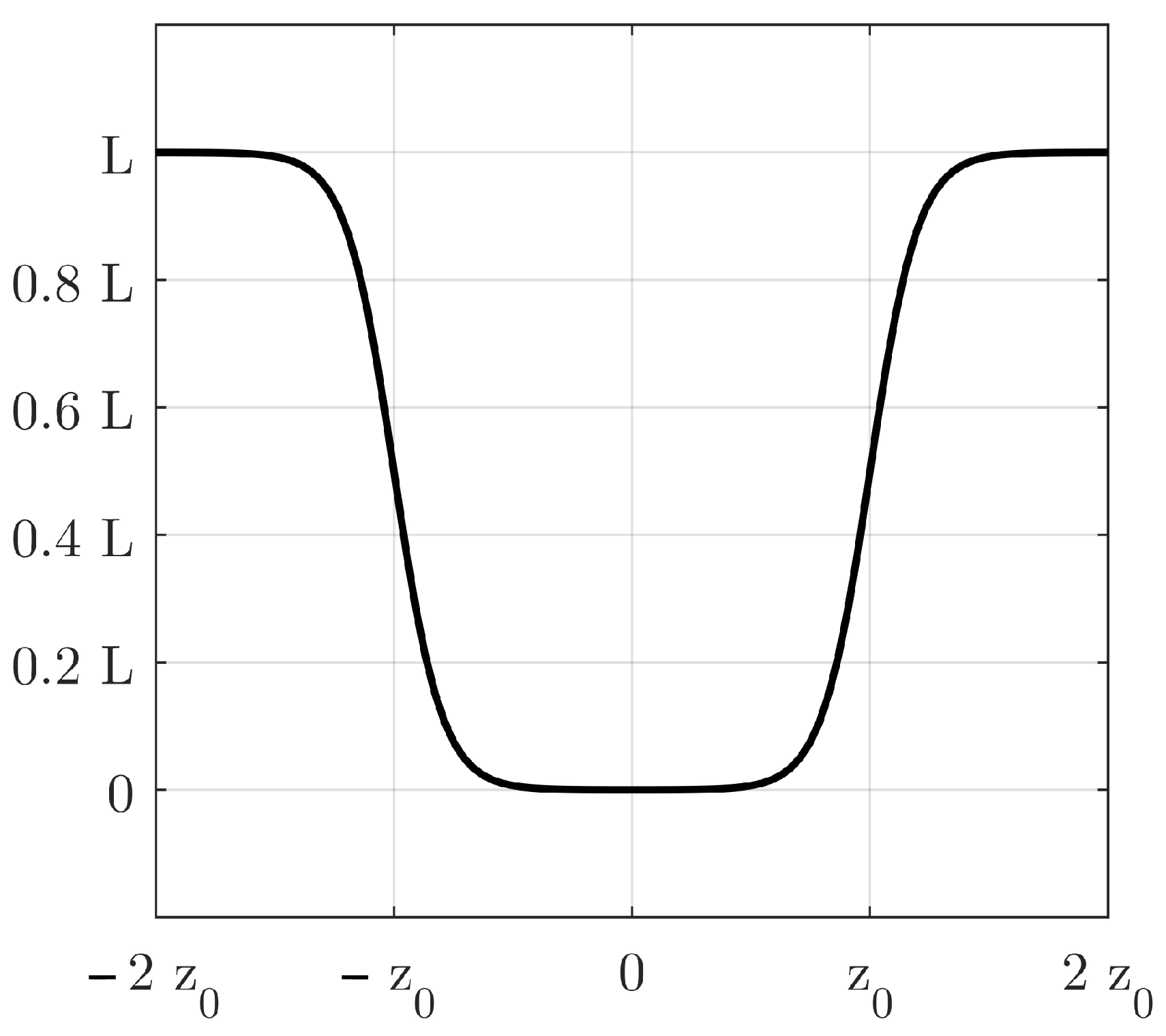
In order to produce a unified dynamic model, the mathematical description of the motion of the tracked vehicle will be modified to include a logistic function (see [37]) and an additional friction coefficient, incorporating both modes of operation to be used for the simulation and to avoid numerical errors around the switching area. This description covers both models of the vehicle, and the transition between models is approximated by sharp but continuous responses, interpreted as friction terms. The switching nature of the model is guaranteed by a rapid decrease in the angular velocity of the vehicle when it enters the first mode of operation. To this end, consider the function:

$$\tilde{f}(\eta ,k,{\eta }_0,L)=L{\left(1+e^{\tilde{k}\left({\eta }_0-\eta \right)}\right)}^{-1}+L{\left(1+e^{\tilde{k}\left({\eta }_0+\eta \right)}\right)}^{-1}$$

(52)

where ${\eta }_0$ defines the flex points of each term in (52), $\tilde{k}$ is a positive real number adjusting the steepness of the curve, and $L$ is a positive real number defining the maximum value of the curve (see Figure 1).

Define $\epsilon (t)=\frac{1}{2}W\left(F_l(t)-F_r(t)\right)$. Using this signal as an argument variable of the above-presented modified logistic function, the two modes of operation of the tracked vehicle are unified, reducing to the respective form of Mode 2, while the linear and angular velocity equations are modified in the form

$$\frac{dv(t)}{dt}=m_t^{-1}\left[F_l(t)+F_r(t)-\left(B_r+B_s\tilde{f}(\epsilon (t),k,S_l,1)\right)v(t)\right],$$

$$\frac{d\omega (t)}{dt}=J_t^{-1}\left\{(W/2)\left(F_l(t)-F_r(t)\right)\tilde{f}(\epsilon (t),k,S_l,1)\left.-\left[B_l+\left(1-\tilde{f}(\epsilon (t),k,S_l,1)\right)B_{\max }\right]\omega (t)\right\}\right.,$$

where $B_{\max }\in {ℝ}^{+}$ is the additional friction term.

Consider the model parameters and the controller parameters presented in Section 4.5. The logistic function parameters, the additional friction term, and the external commands amplitudes are selected to be

$$\begin{gathered} T_{1,1}=0.2, T_{1,2}=0.3, T_{1,3}=0.4, T_{2,1}=1.5, T_{2,2}=1.7, T_{2,3}=1.9, {\tau }_1=0\left[\mathrm{s}\right], {\tau }_2=8\left[\mathrm{s}\right], \\ \tilde{k}=8, S_l=0.3\left[\mathrm{Nm}\right], B_{\max }=0.7\left[\mathrm{Nms}/\mathrm{rad}\right], {\tilde{w}}_1=0.02\left[\mathrm{m}/\mathrm{s}\right], {\tilde{w}}_2=\pi \left[\mathrm{rad}\right]. \end{gathered}$$

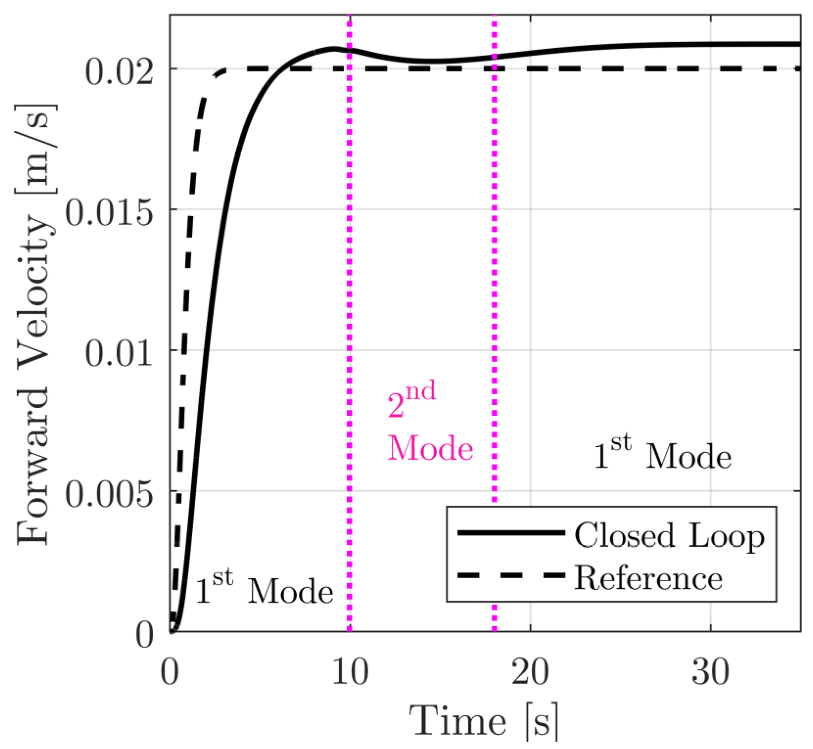
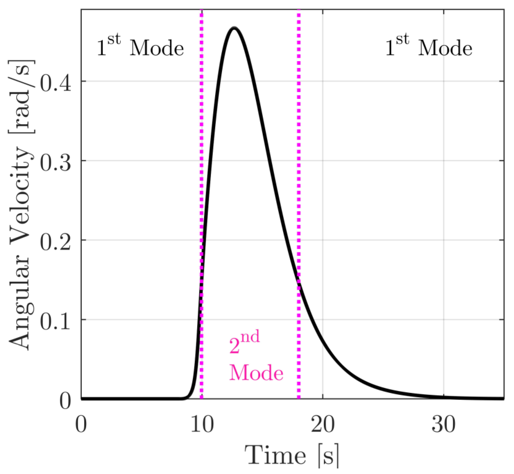
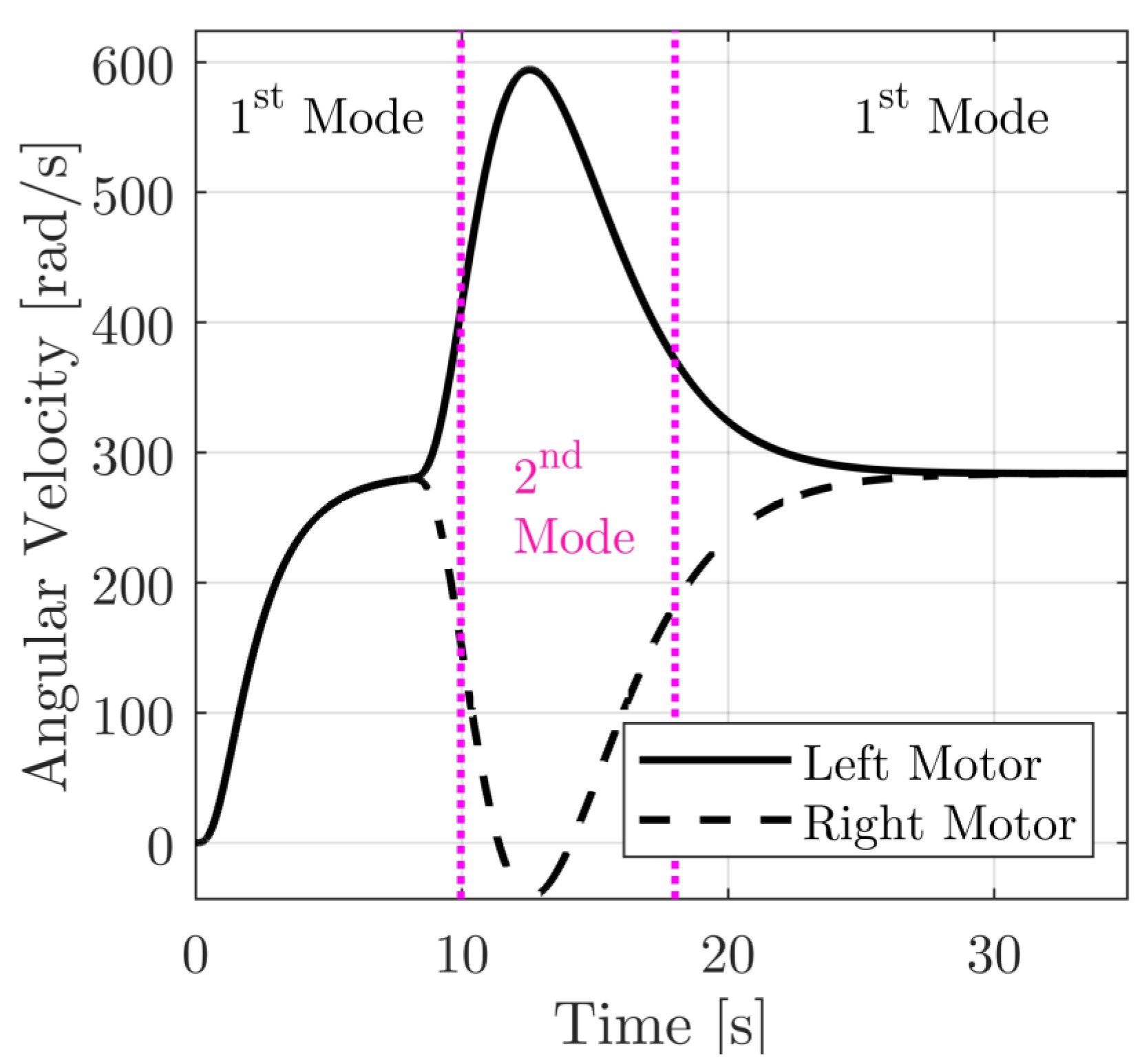
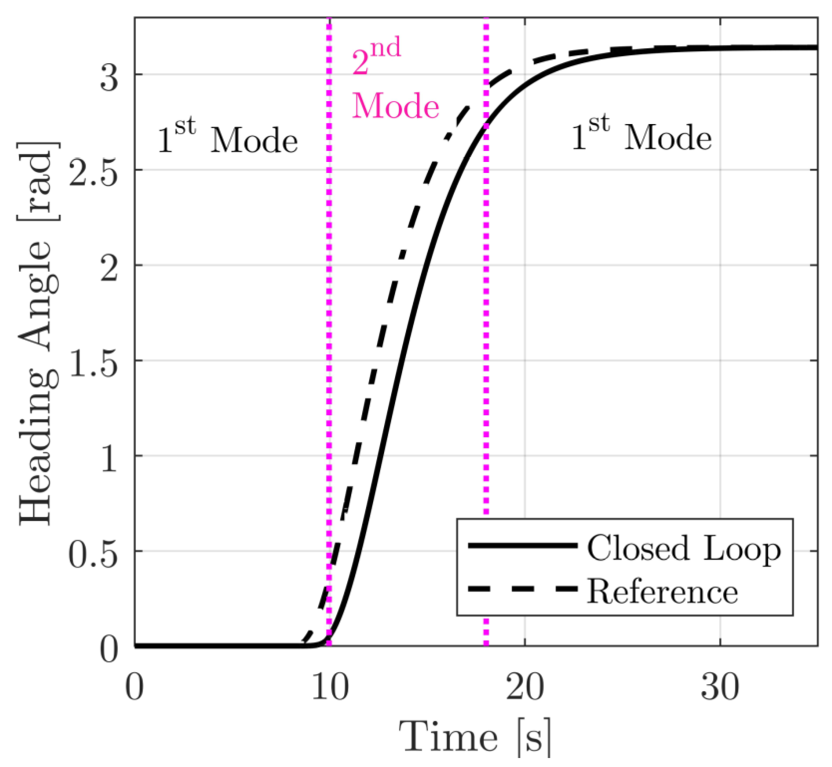
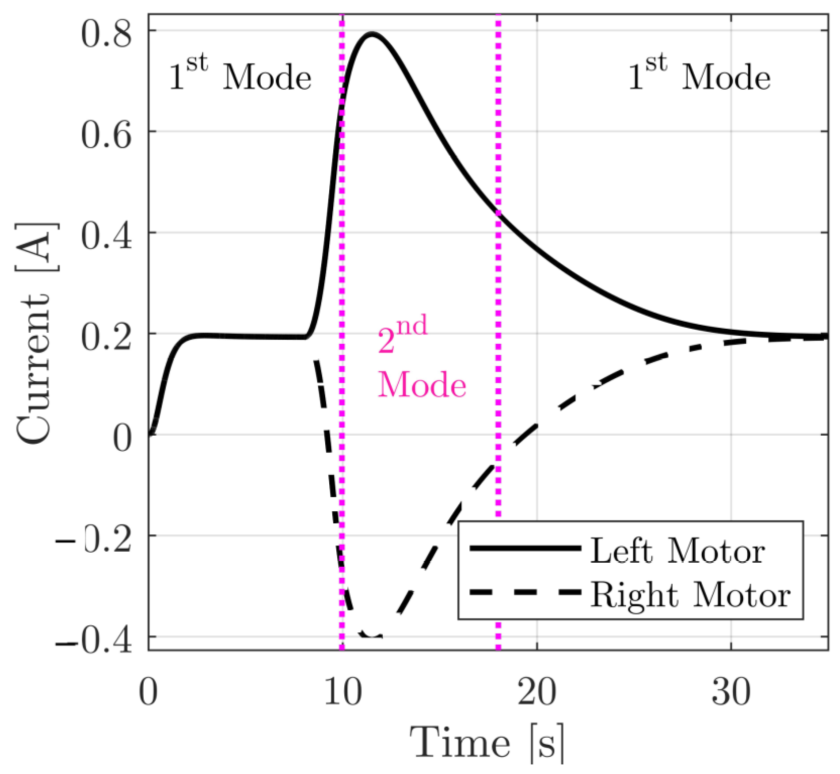
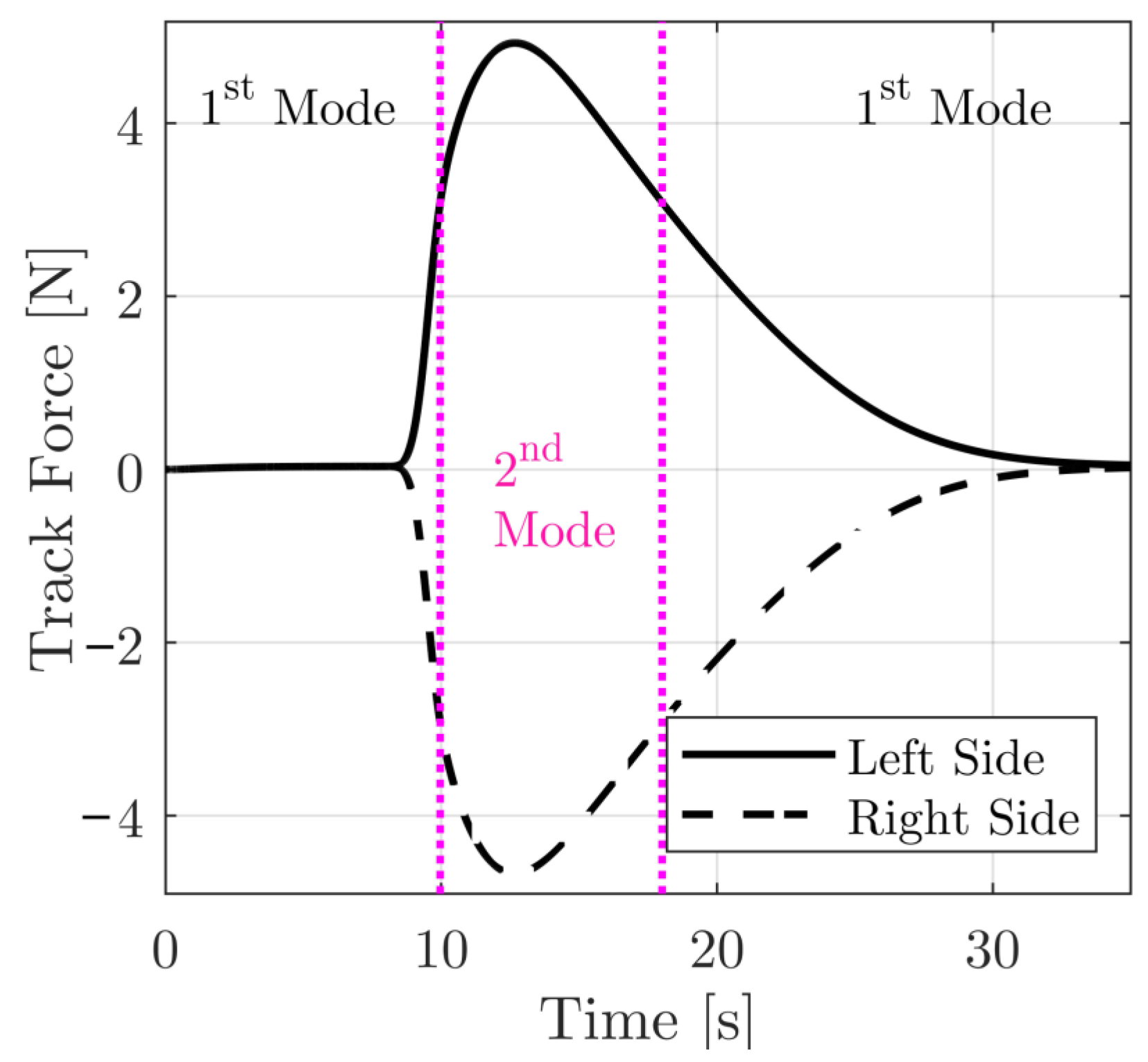
Figure 2, Figure 3, Figure 4, Figure 5, Figure 6 and Figure 7 present the simulation results for the robot-tracked vehicle’s closed-loop response. 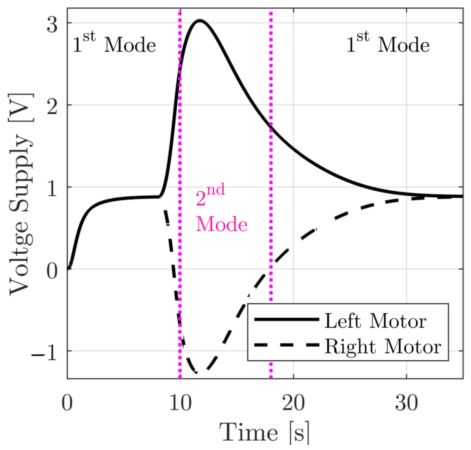In particular, in Figure 2 and Figure 3, the forward and angular velocities are presented, respectively; in Figure 4, the heading angle is presented; in Figure 5 and Figure 6, the motor currents and angular velocities are presented; in Figure 7, the track forces are presented; and, in Figure 8, the voltage supply to the motors of the vehicle are presented. With respect to the performance variables $x_1$ and $x_3$, it can be verified that the external commands are followed accurately (see Figure 2 and Figure 4). With respect to the voltage supply to the electric motors (see Figure 8), it is observed that they are smooth and appropriately bounded, being easily implementable. Note that the voltage supplies, motor currents, and motor velocities are within the respective technical specifications of the motor. For more details, see the Data Sheet of the FA-130 Mabuchi Motor and [16]. Besides, the performance outputs, the remaining state variables (see Figure 3, Figure 5, Figure 6 and Figure 7) are appropriately bounded.

To demonstrate the effectiveness of the proposed control scheme, with respect to uncertainties, what follows will be considered the mechanical resistances of the tracks to rolling ($B_r$ and $B_s$) and the mechanical resistance of sliding forward ($B_l$). Moreover, the mechanical resistance of the gears to rotation ($B_g$) and the lateral friction of the tracks ($S_l$) are not perfectly known to the designer. So, these parameters are considered to be uncertain, and they are expressed as follows: $B_r=B_{r,0}+\delta B_r$, $B_s=B_{s,0}+\delta B_s$, $B_l=B_{l,0}+\delta B_l$, $B_g=B_{g,0}+\delta B_g$, and $S_l=S_{l,0}+\delta S_l$, where $B_{r,0}$, $B_{s,0}$, $B_{l,0}$, $B_{g,0}$, and $S_{l,0}$ are the respective nominal values of the parameters upon which the controller was evaluated, and where $\delta B_r$, $\delta B_s$, $\delta B_l$, $\delta B_g$, and $\delta S_l$ are the respective uncertainties. Let $y_{1,0}(t)$ and $y_{2,0}(t)$ be the nonlinear closed-loop responses of the performance variables. As already mentioned, the controller is designed using the parameters $B_{r,0}$, $B_{s,0}$, $B_{l,0}$, $B_{g,0}$, and $S_{l,0}$ instead of their real values. Furthermore, it is mentioned that the external commands and the rest model parameters are chosen as in the previous paragraphs. Finally, let $y_1(t)$ and $y_2(t)$ be the closed-loop response of the performance variables produced after applying the controller to the original uncertain system. The following metrics will be used to compare the respective responses:

$${\epsilon }_{2,j}=\frac{{‖y_j(t)-y_{j,0}(t)‖}_2}{{‖y_{j,0}(0-)-y_{j,0}(t)‖}_2}\times 100\%,{\epsilon }_{\infty ,j}=\frac{{‖y_j(t)-y_{j,0}(t)‖}_{\infty }}{{‖y_{j,0}(0-)-y_{j,0}(t)‖}_{\infty }}\times 100\%; j=1,2,$$

where ${‖\eta (t)‖}_2$ and ${‖\eta (t)‖}_{\infty }$ denote the finite horizon 2-norm and infinity norm (indicatively, see [38,39]) of the argument signal $\eta (t)$, i.e., it holds that

$${‖\eta (t)‖}_2^2={\displaystyle \underset{0}{\overset{T_{\max }}{\int }}\eta {(\rho )}^{2}d\rho }, {‖\eta (t)‖}_{\infty }=\underset{t\in \left[0,T_{\max }\right]}{\sup }\left|\eta (t)\right|,$$

where $T_{\max }$ denotes computational experiment simulation time. For demonstration purposes, it will be assumed that $T_{\max }=35[s]$.

Performing a series of computational experiments for $\delta B_r\in \left[-p_{\delta }{B}_{r,0},p_{\delta }{B}_{r,0}\right]$, $\delta B_s\in \left[-p_{\delta }{B}_{s,0},p_{\delta }{B}_{s,0}\right]$, $\delta B_l\in \left[-p_{\delta }{B}_{l,0},p_{\delta }{B}_{l,0}\right]$, $\delta B_g\in \left[-p_{\delta }{B}_{g,0},p_{\delta }{B}_{g,0}\right]$, and $\delta S_l\in \left[-p_{\delta }{S}_{l,0},p_{\delta }{S}_{l,0}\right]$, where $p_{\delta }=0.1$, it was observed that the second performance variable, namely the heading angle of the vehicle, is minimally affected by the presence of the uncertainties. The maximum values of ${\epsilon }_{2,2}$ and ${\epsilon }_{\infty ,2}$ were found to be $0.2191\%$ and $0.3483\%$. Regarding the first performance variable, namely the speed of the UGV, it is observed that the uncertainties affect the closed-loop response at acceptable levels. The maximum values of ${\epsilon }_{2,1}$ and ${\epsilon }_{\infty ,1}$ were computed to be $11.2467\%$ and $12.8360\%$, respectively. In

Table 1. Maximum metric values for different $p_{\delta }$.

${\mathit{p}}_{\mathit{\delta }}$	$\mathbf{max}\left\{{\mathit{\epsilon }}_{2,1}\right\}$	$\mathbf{max}\left\{{\mathit{\epsilon }}_{2,2}\right\}$	$\mathbf{max}\left\{{\mathit{\epsilon }}_{\mathit{\infty },1}\right\}$	$\mathbf{max}\left\{{\mathit{\epsilon }}_{\mathit{\infty },2}\right\}$
0.03	3.5230%	0.0560%	4.8904%	0.0849%
0.04	4.9616%	0.0770%	6.3766%	0.1224%
0.05	5.9344%	0.1047%	7.3629%	0.1646%
0.06	6.9410%	0.1359%	8.4145%	0.2135%
0.07	8.0160%	0.1482%	9.5019%	0.2332%
0.08	9.1177%	0.1771%	10.6154%	0.2763%
0.09	10.1815%	0.2019%	11.7400%	0.3115%
0.10	11.2467%	0.2191%	12.8360%	0.3483%

, the maximum values of ${\epsilon }_{2,1}$, ${\epsilon }_{2,2}$, ${\epsilon }_{\infty ,1}$, and ${\epsilon }_{\infty ,2}$ are presented for different values of $p_{\delta }$. The present simulation results demonstrate some of the perspectives of the proposed controller in a real environment.

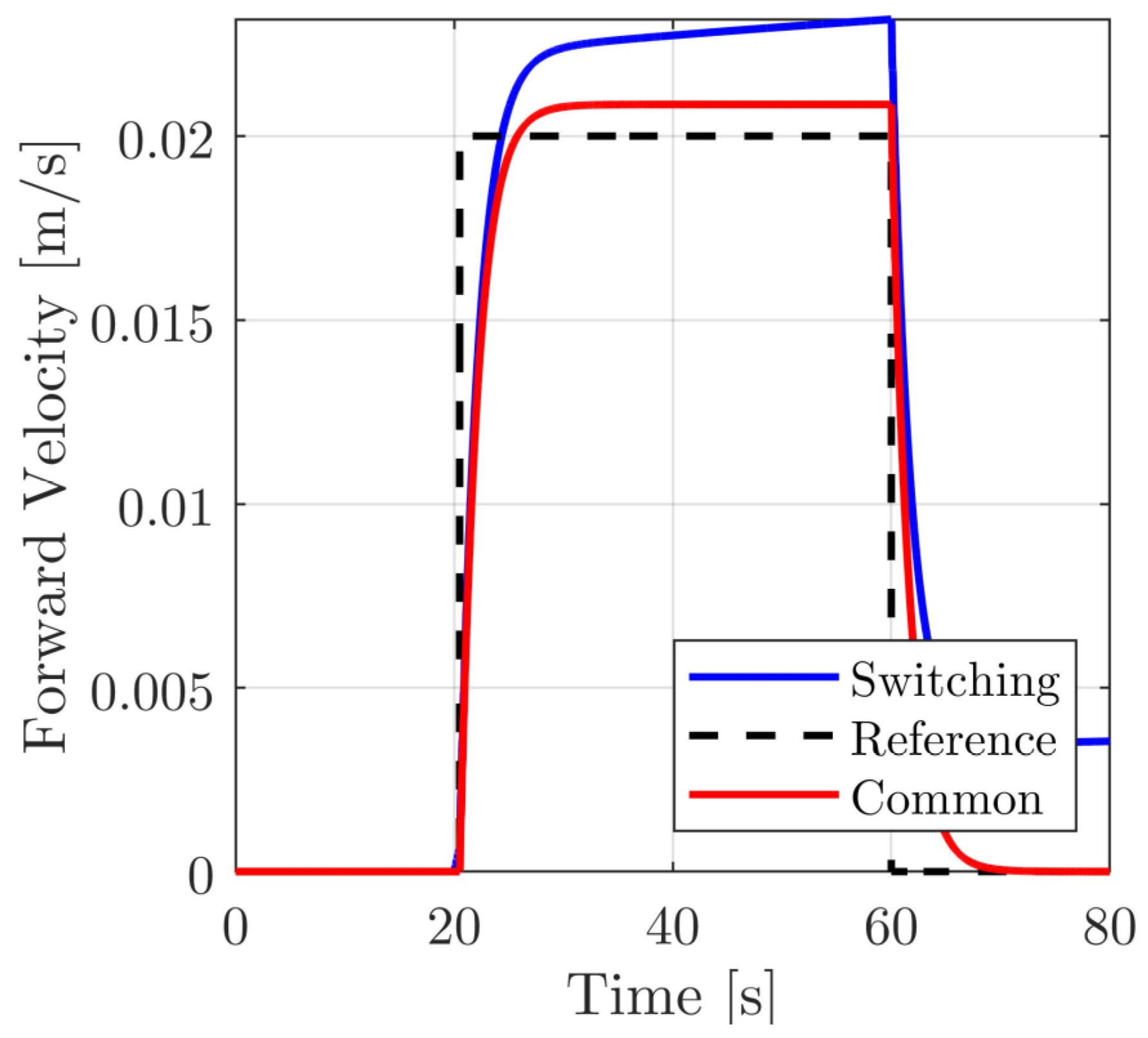
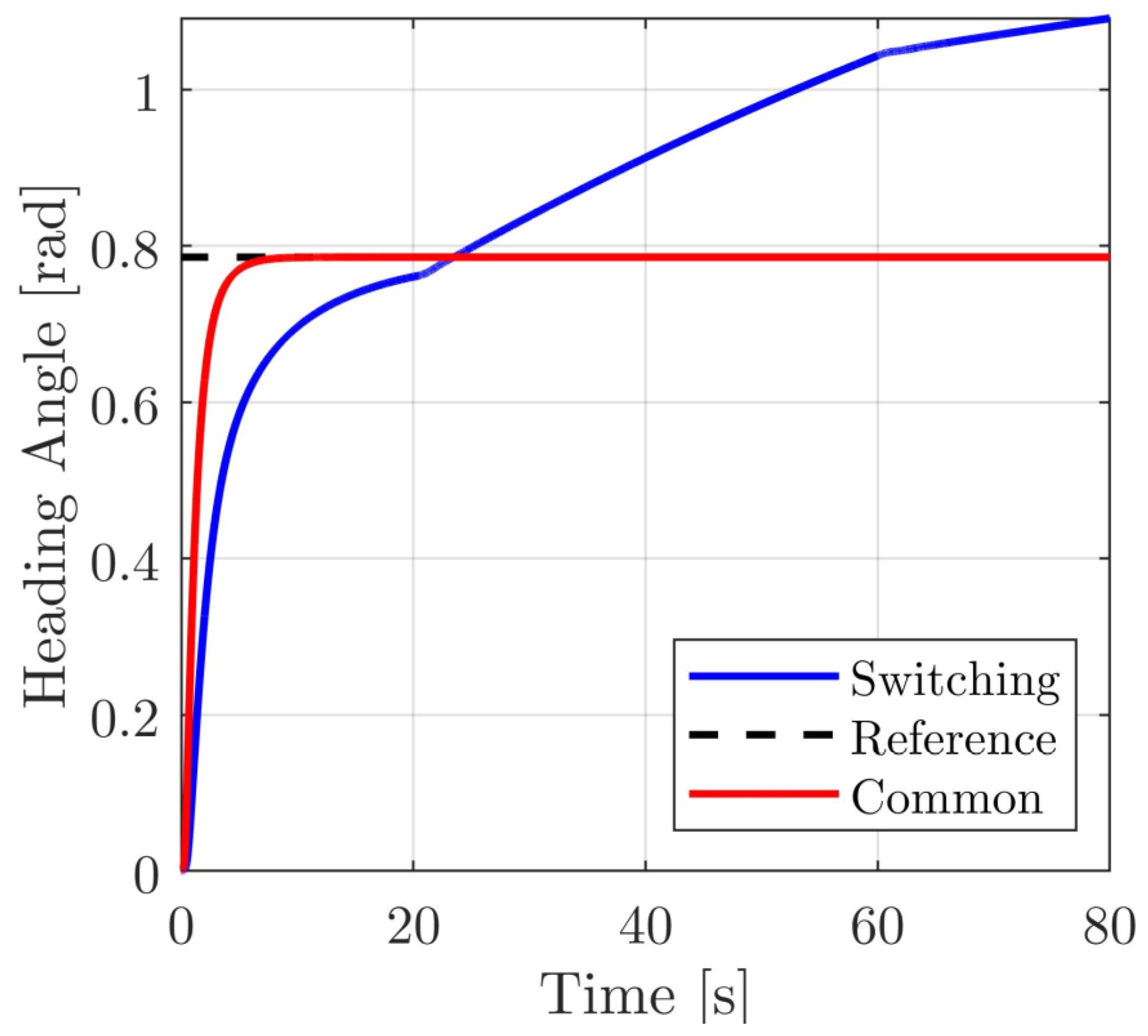
4.7. Comparison to Switching Controllers

In this subsection, the common control design scheme derived in the previous subsections for the robot-tracked UGV is compared to a switching control design scheme satisfying the same design requirements with two different controllers, one for each mode of the UGV. These two controllers are switched by the external commands and measurement of the heading angle of the vehicle, in the sense that the first is triggered when the external vector command corresponds to a straight path and constant heading angle, while the second is triggered when the external vector command corresponds to a curved path. The curved path period is completed, and consequently, the straight path controller is switched on when the heading angle has reached 97% of the final value of its variation. Clearly, this time period covers the settling time of the heading angle.

Regarding the design requirements of the switching scheme, the first requirement is to satisfy (51), i.e., the first controller satisfies the first equality in (51), while the second controller satisfies the second equality in (51). Following Remark 2 for $N=1$, the following general forms of the controller matrices are derived:

$$F_M\left(1\right)=\left[\begin{array}{ccc}{f}_{1,1}\left(1\right)& f_{1,3}\left(1\right)-f_{2,2}\left(1\right)+f_{2,3}\left(1\right)& f_{1,3}\left(1\right)\\ f_{2,1}\left(1\right)& f_{2,2}\left(1\right)& f_{2,3}\left(1\right)\end{array}\right],$$

$$G\left(1\right)=\left[\begin{array}{cc}\frac{2g\alpha }{r}+\frac{\left(2g^2{B}_g+r^2{B}_r\right)\left(R_m-f_{1,3}\left(1\right)-f_{2,3}\left(1\right)\right)}{r\alpha g}-g_{2,1}\left(1\right)& -g_{2,2}\left(1\right)\\ g_{2,1}\left(1\right)& g_{2,2}\left(1\right)\end{array}\right],$$

$$F_M\left(2\right)=\left[\begin{array}{ccc}-f_{2,1}\left(2\right)& f_{2,3}\left(2\right)& f_{1,3}\left(2\right)\\ f_{2,1}\left(2\right)& f_{1,3}\left(2\right)& f_{2,3}\left(2\right)\end{array}\right], G\left(2\right)=\left[\begin{array}{cc}{g}_{2,1}\left(2\right)& -g_{2,2}\left(2\right)\\ g_{2,1}\left(2\right)& g_{2,2}\left(2\right)\end{array}\right],$$

where $f_{i,j}\left(k\right)$ and $g_{l,q}\left(k\right)$ are the $\left\{i,j\right\}$ and $\left\{l,q\right\}$ elements of the feedback and precompensator matrices, respectively, for $k\in \{1,2\}$. The free elements of the feedback matrices $F_M\left(1\right)$ and $F_M\left(2\right)$, i.e., the elements $f_{1,1}\left(1\right)$, $f_{1,3}\left(1\right)$, $f_{2,1}\left(1\right)$, $f_{2,2}\left(1\right)$, $f_{2,3}\left(1\right)$, $f_{1,3}\left(2\right)$, $f_{2,1}\left(2\right)$, and $f_{2,3}\left(2\right)$, will be chosen such that the eigenvalues of the matrices $A\left(k\right)+B\left(k\right)F_M\left(k\right)C_m\left(k\right)$ ($k=1,2$) are stable. The free elements of the precompensator matrices $G\left(1\right)$ and $G\left(2\right)$, i.e., the elements $g_{2,1}\left(1\right)$, $g_{2,2}\left(1\right)$, $g_{2,1}\left(2\right)$, and $g_{2,2}\left(2\right)$, must be chosen such that $\det \left\{G\left(k\right)\right\}\ne 0$, $\forall k\in \{1,2\}$. In addition to the above constraints, the asymptotic command following is also achieved for the nonzero elements for the closed-transfer matrices of the two modes. In what follows, the determination of the free controller matrix elements will be carried out through the metaheuristic algorithm mentioned in Section 4.5, where the model parameters are those presented in Section 4.5. After applying a series of computations, the two sets of controller matrices are determined to be

$$F_M\left(1\right)=\left[\begin{array}{ccc}0.6068& -83.8709& -26.9298\\ 3.0716& 27.4905& -29.4506\end{array}\right], G\left(1\right)=\left[\begin{array}{cc}1114.9475& 4.9730\\ 0.5969& -4.9730\end{array}\right],$$

$$F_M\left(2\right)=\left[\begin{array}{ccc}-0.6522& -23.4586& -25.7426\\ 0.6522& -25.7426& -23.4586\end{array}\right], G\left(2\right)=\left[\begin{array}{cc}519.0108& 0.6522\\ 519.0108& -0.6522\end{array}\right].$$

Here, the simulations are performed with zero initial conditions. Furthermore, the two external commands are chosen to be

$$w_1(t)=\{\begin{array}{cc}0& 0\left[\mathrm{s}\right]\le t<20.5\left[\mathrm{s}\right]\\ 0.02u_s\left(t\right)& 20.5\left[\mathrm{s}\right]\le t<60\left[\mathrm{s}\right]\\ 0& t\ge 60\left[\mathrm{s}\right]\end{array}, w_2(t)=\frac{\pi }{4}{u}_s\left(t\right).$$

The simulations begin with the second controller of the switching scheme. At $t=20.5[s]$ the heading angle has reached the 97% of its final value, i.e., $0.762\left[\mathrm{rad}\right]$, and so the first controller is switched on. From that point on, since no change in the orientation command is imposed, the straight path controller of the switching scheme is preserved. The closed-loop responses of the performance outputs for both the common controller case and the switching controller case are presented in Figure 9 and Figure 10, where it is observed that, for the present metaheuristic evaluation of the controller-free parameters, the closed-loop response of the common controller is preferable as compared to the switching controller. Indicatively, consider the performance metric ${\epsilon }_i={‖y_i(t)-w_i(t)‖}_2$, $i=1,2$. According to the simulation results, in the common controller case, the metric is evaluated to be ${\epsilon }_1=0.0263$ and ${\epsilon }_2=0.7263$, while in the switching controller case, the metric is evaluated to be ${\epsilon }_1=0.037$ and ${\epsilon }_2=1.9509$.

5. Discussion

In its general form, the problem of common noninteracting control with simultaneous common partial output zeroing is applicable in the sense that some of the outputs are independently controlled while some of them are retained at their nominal values. Such a requirement can be met in redundant manipulators, multi-mode processes, and robotic vehicles.

The approach followed to solve the problem at hand is purely algebraic, facilitating the computation of the quantities in the solvability criteria as well as the general solution of the controller.

The application of the present results to the case of a UGV is quite useful and provides useful insight into the properties of the problem at hand. From the point of view of the availability of measurements, the measurement variables used by the controller appear to be the preferable choice.

Significant issues, such as the switching stability of the controlled UGV and the robustness of the derived results with respect to measurement noise, are currently under investigation.

A future perspective of the results of the present paper is the extension to other problems in the wider class of noninteracting control; indicatively, see the common noninteracting control problems in [40,41], as well as the seminal works in [42,43,44], where pure noninteracting control problems are studied for nonsquare systems with static controllers, including nonsquare precompensators.

6. Conclusions

The problem of common noninteracting control with simultaneous partial output zeroing for normal linear time-invariant multi-model systems was introduced and formulated. The problem was solved using regular and static measurement output feedback type controllers. The necessary and sufficient conditions for the solvability of the problem were established. The general solution of the feedback matrix and the precompensator matrix of the controller, solving the problem at hand, were determined in purely algebraic analytic forms, including a set of free parameters. These free parameters were used to achieve an approximate command following with simultaneous I/O stabilizability.

The above results were applied to a two-model robot-tracked UGV, using a common controller feeding back the motor currents and the heading angle of the UGV. The set of the free parameters of the controller of the UGV is determined by the application of a metaheuristic algorithm to improve the transient behaviors of the closed-loop system.

References

1. Koumboulis, F.N.; Kouvakas, N.D. A Common Noninteracting Control Design for Robot Tracked Vehicles. In Proceedings of the 30th Mediterranean Conference on Control and Automation (MED), Vouliagmeni, Greece, 28 June–1 July 2022. [Google Scholar] [CrossRef]
2. Vidyasagar, M. A state–space interpretation of simultaneous stabilization. IEEE Trans. Autom. Control. 1988, 33, 506–508. [Google Scholar] [CrossRef]
3. Rotea, M.A.; Viassolo, D.E. On a sufficient condition for static output feedback multimodel control. In Proceedings of the 2001 American Control Conference, Arlington, VA, USA, 25–27 June 2001. [Google Scholar] [CrossRef]
4. Moreno, J.A. Simultaneous observation of linear systems: A state-space interpretation. IEEE Trans. Autom. Control. 2005, 50, 1021–1025. [Google Scholar] [CrossRef]
5. Koumboulis, F.N. On the heuristic design of common PI controllers for multi-model plants. In Proceedings of the 2005 IEEE Conference on Emerging Technologies and Factory Automation, Catania, Italy, 19–22 September 2005. [Google Scholar] [CrossRef]
6. Trinh, H.; Fernando, T. Design of a Common Observer for Two Linear Systems with Unknown Inputs. In Proceedings of the TENCON 2006—2006 IEEE Region 10 Conference, Hong Kong, China, 14–17 November 2006. [Google Scholar] [CrossRef] [Green Version]
7. Kim, S.; Moon, Y.; Kwon, S. Simultaneous stabilization by static output feedback: A rank-constrained LMI approach. In Proceedings of the 45th IEEE Conference on Decision and Control, San Diego, CA, USA, 13–15 December 2006. [Google Scholar] [CrossRef]
8. Trinh, H.; Teh, P.S.; Ha, Q.P. A common disturbance decoupled observer for linear systems with unknown inputs. Int. J. Autom. Control. 2008, 2, 286–297. [Google Scholar] [CrossRef]
9. Koumboulis, F.N. Common I/O Decoupling for Multi Model Descriptor Systems. IEEE Trans. Autom. Control. 2016, 61, 783–788. [Google Scholar] [CrossRef]
10. Koumboulis, F.N. A Unified approach for Common I/O decoupling via measurement output feedback of multi model descriptor systems. J. Frankl. Inst. 2016, 353, 4253–4279. [Google Scholar] [CrossRef]
11. Koumboulis, F.N. On the Common Control Design of Robotic Manipulators Carrying Different Loads. In Advances in Service and Industrial Robotics—(RAAD 2018); Aspragathos, N., Koustoumpardis, P., Moulianitis, V., Eds.; Springer International Publishing: Cham, Switzerland, 2019; pp. 416–424. [Google Scholar] [CrossRef]
12. Koumboulis, F.N.; Tzamtzi, M.P. A Metaheuristic Approach for Controller Design of Multivariable Processes. In Proceedings of the 12th IEEE Conference on Emerging Technologies and Factory Automation, Patras, Greece, 25–28 September 2007. [Google Scholar] [CrossRef]
13. Koumboulis, F.N.; Tzamtzi, M.P. A generalised control metaheuristic framework for industrial processes. Int. J. Autom. Control. 2010, 4, 218–233. [Google Scholar] [CrossRef]
14. Koumboulis, F.N.; Kucera, V. Partial Model Matching via Static Feedback (The Multivariable Case). IEEE Trans. Autom. Control. 1999, 44, 386–392. [Google Scholar] [CrossRef]
15. Le, A.T. Modelling and Control of Tracked Vehicles. Ph.D. Thesis, Department of Mechanical and Mechatronic Engineering, University of Sydney, Camperdown, NSW, Australia, 1999. [Google Scholar]
16. Nutaro, J.J. Building Software for Simulation: Theory and Algorithms, with Applications in C++; John Wiley & Sons Inc: Hoboken, NJ, USA, 2011. [Google Scholar]
17. Ferretti, G.; Girelli, R. Modelling and Simulation of an agricultural tracked vehicle. J. Terramech. 1999, 36, 139–158. [Google Scholar] [CrossRef]
18. Mocera, F.; Nicolini, A. Multibody Simulation of a Small Size Farming tracked vehicle. Procedia Struct. Integr. 2018, 8, 118–125. [Google Scholar] [CrossRef]
19. Das, R.K.; Upadhyay, A.; Garg, R.K. An Unmanned Tracked Vehicle for Snow Research Applications. Def. Sci. J. 2017, 67, 74–79. [Google Scholar] [CrossRef] [Green Version]
20. Sebastian, B.; Ben-Tzvi, P. Physics Based Path Planning for Autonomous Tracked Vehicle in Challenging Terrain. J. Intell. Robot. Syst. 2019, 95, 511–526. [Google Scholar] [CrossRef]
21. Dai, Y.; Zhu, X.; Zhou, H.; Mao, Z.; Wu, W. Trajectory Tracking Control for Seafloor Tracked Vehicle by Adaptive Neural-Fuzzy Inference System Algorithm. Int. J. Comput. Commun. Control. 2018, 13, 465–476. [Google Scholar] [CrossRef] [Green Version]
22. Zweiri, Y.H.; Seneviratne, L.D.; Althoefer, K. Modelling and control of an unmanned excavator vehicle. Proc. Inst. Mech. Eng. Part I J. Syst. Control. Eng. 2003, 217, 259–274. [Google Scholar] [CrossRef]
23. Zou, Y.; Zhang, C.; Sun, F.; Wu, J. Power control of dual-motor electric drive for tracked vehicles. Front. Mech. Eng. China 2010, 5, 67–72. [Google Scholar] [CrossRef]
24. Subari, M.A.; Hudha, K.; Abd Kadir, Z.; Dardin, S.M.F.B.S.M.; Amer, N.H. Development of path tracking control of a tracked vehicle for an unmanned ground vehicle. Int. J. Adv. Mechatron. Syst. 2020, 8, 136–143. [Google Scholar] [CrossRef]
25. Sidi, M.H.A.; Hudha, K.; Kadir, Z.A.; Amer, N.H. Modeling and path tracking control of a tracked mobile robot. In Proceedings of the 2018 IEEE 14th Int. Colloquium on Signal Processing & Its Applications (CSPA), Penang, Malaysia, 9–10 March 2018. [Google Scholar] [CrossRef]
26. Gonzalez, R.; Fiacchini, M.; Alamo, T.; Guzman, J.L.; Rodriguez, F. Adaptive Control for a Mobile Robot Under Slip Conditions Using an LMI-Based Approach. Eur. J. Control. 2010, 16, 144–155. [Google Scholar] [CrossRef]
27. Gonzalez, R.; Rodriguez, F.; Guzman, J.L.; Berenguel, M. Localization and control of tracked mobile robots under slip conditions. In Proceedings of the 2009 IEEE International Conference on Mechatronics, Malaga, Spain, 14–17 April 2009. [Google Scholar] [CrossRef]
28. Zou, T.; Angeles, J.; Hassani, F. Dynamic modeling and trajectory tracking control of unmanned tracked vehicles. Robot. Auton. Syst. 2018, 110, 102–111. [Google Scholar] [CrossRef]
29. Sabiha, A.D.; Kamel, M.A.; Said, E.; Hussein, W.M. ROS-based trajectory tracking control for autonomous tracked vehicle using optimized backstepping and sliding mode control. Robot. Auton. Syst. 2022, 152, 102–111. [Google Scholar] [CrossRef]
30. Sabiha, A.D.; Kamel, M.A.; Said, E.; Hussein, W.M. Dynamic modeling and optimized trajectory tracking control of an autonomous tracked vehicle via backstepping and sliding mode control. Proc. Inst. Mech. Eng. Part I J. Syst. Control. Eng. 2022, 236, 620–633. [Google Scholar] [CrossRef]
31. Kuwahara, H.; Murakami, T. Position Control Considering Slip Motion of Tracked Vehicle Using Driving Force Distribution and Lateral Disturbance Suppression. IEEE Access 2022, 10, 20571–20580. [Google Scholar] [CrossRef]
32. Han, J.; Fan, W.; Wang, Y. A control method for the differential steering of tracked vehicles driven independently by a dual hydraulic motor. Appl. Sci. 2022, 12, 6355. [Google Scholar] [CrossRef]
33. Al-Jarrah, A.; Salah, M. Trajectory tracking control of tracked vehicles considering nonlinearities due to slipping while skid-steering. Syst. Sci. Control. Eng. 2022, 10, 887–898. [Google Scholar] [CrossRef]
34. Giannaris, G.L.; Kouvakas, N.D.; Koumboulis, F.N.; Vouyioukas, D. Switching Wireless Control for Longitudinal Quadrotor Maneuvers. J. Intell. Robot. Syst. 2021, 102, 1–21. [Google Scholar] [CrossRef]
35. Suzuki, T.; Kanada, T. Measurement of vehicle motion and orientation using optical flow. In Proceedings of the IEEE/IEEJ/JSAI International Conference on Intelligent Transportation Systems, Tokyo, Japan, 5–8 October 1999. [Google Scholar] [CrossRef]
36. Kuo, B.C. Automatic Control Systems; Prentice Hall International Editions: Hoboken, NJ, USA, 1991. [Google Scholar]
37. Kyurkchiev, N.; Markov, S. On the Hausdorff distance between the Heaviside step function and Verhulst logistic function. J. Math. Chem. 2016, 54, 109–119. [Google Scholar] [CrossRef]
38. Doyle, J.C.; Francis, B.A.; Tannenbaum, A.R. Feedback Control Theory; Macmillan Publishing Co.: New York, NY, USA, 1990. [Google Scholar]
39. Zhou, K.; Doyle, J.C.; Glover, K. Robust and Optimal Control; Prentice Hall: Hoboken, NJ, USA, 1996. [Google Scholar]
40. Koumboulis, F.N. P-D state feedback controllers for common I/O decoupling of multi model descriptor systems. In Proceedings of the 24th Mediterranean Conference on Control and Automation (MED), Athens, Greece, 21–24 June 2016. [Google Scholar] [CrossRef]
41. Koumboulis, F.N. On the PD State Feedback Controller Design for the Common Triangular Decoupling of Multi Model Descriptor Systems. In Proceedings of the 7th International Conference on Systems and Control, Valencia, Spain, 24–26 October 2018. [Google Scholar] [CrossRef]
42. Kučera, V. Diagonal Decoupling of Linear Systems by Static-State Feedback. IEEE Trans. Autom. Control. 2017, 62, 6250–6265. [Google Scholar] [CrossRef]
43. Kučera, V. Block Decoupling of Linear Systems by Static-State Feedback. IEEE Trans. Autom. Control. 2019, 64, 3447–3452. [Google Scholar] [CrossRef]
44. Kučera, V. Decoupling With Stability of Linear Systems by Static-State Feedback. IEEE Trans. Autom. Control. 2021, 66, 4684–4699. [Google Scholar] [CrossRef]
Figure 1. Modified logistic function.
Machines 11 00113 g001
Figure 2. Forward velocity of the vehicle.
Machines 11 00113 g002
Figure 3. Angular velocity of the vehicle.
Machines 11 00113 g003
Figure 4. Heading angle of the vehicle.
Machines 11 00113 g004
Figure 5. Motor currents.
Machines 11 00113 g005
Figure 6. Motor angular velocities.
Machines 11 00113 g006
Figure 7. Track forces.
Machines 11 00113 g007
Figure 8. Voltage supplies.
Machines 11 00113 g008
Figure 9. Forward velocity of the vehicle.
Machines 11 00113 g009
Figure 10. Heading angle of the vehicle.
Machines 11 00113 g010