Ensemble Classifier for Recognition of Small Variation in X-Bar Control Chart Patterns

Abstract

Manufacturing processes have become highly accurate and precise in recent years, particularly in the chemical, aerospace, and electronics industries. This has attracted researchers to investigate improved procedures for monitoring and detection of small process variations to remain in line with such advances. Among these techniques, statistical process controls (SPC), in particular the control chart pattern (CCP), have become a popular choice for monitoring process variance, being utilized in numerous industrial and manufacturing applications. This study provides an improved control chart pattern recognition (CCPR) method focusing on X-bar chart patterns of small process variations using an ensemble classifier comprised of five complementing algorithms: decision tree, artificial neural network, linear support vector machine, Gaussian support vector machine, and k-nearest neighbours. Before advancing to the classification step, Nelson’s Rus Rules were utilized as a monitoring rule to distinguish between stable and unstable processes. The study’s findings indicate that the proposed method improves classification performance for patterns with mean changes of less than 1.5 sigma, and confirm that the performance of the ensemble classifier is superior to that of the individual classifier. The ensemble classifier can distinguish unstable pattern types with a classification accuracy of 99.55% and an ARL1 of 11.94.

1. Introduction

These days, the competition among manufacturing companies is increasingly oriented towards quality, with the end goal being to produce a product that is of the best possible quality. Manufacturing processes have become highly accurate and precise, particularly in the chemical, aerospace, and electronics industries. This has attracted researchers to investigate improved procedures for monitoring and detection of small process variation in order to be in line with such advances [1,2]. Manufacturing companies are using advanced technologies for quality control, such as artificial intelligence and control chart pattern recognition (CCPR). CCPR is regarded as one of the most important statistical process control (SPC) techniques. The implementation of CCPR with suitable algorithms has gained importance due to its capability to recognize unstable processes. In addition, it can provide operators with early warning, allowing for preventive action to avoid production of defective products. CCPR gains its popularity because it provides useful hints for locating the source of process variation. This is valuable for industrial practitioners such as quality inspectors and production supervisors in determining the root causes of various problems. A particular CCP can be associated with the potential origin of process variation [3,4,5]. Such variability may be attributed to human faults, defective manufacturing equipment, broken tools, or defective materials, among others. When a process is out of control, process behavior can take on a number of unnatural patterns on an X-bar chart, including the trend (UT), descending trend (DT), stratification (STA), downward shift (DS), cyclic (CYC), systemic (SYS), upward shift (US), and mixed patterns (MIX) [6,7,8,9,10,11].

Researchers have proposed various designs for CCPR schemes. Several scholars have introduced improved input data representation by extracting features from raw data, such as wavelet features, statistical features, and shape features [12,13]. Selection of suitable essential input features can increase the efficiency of CCPR schemes [14,15]. Kim [16] investigated ways to reduce the number of feature dimensions using principal component analysis (PCA). PCA is a fundamental tool in statistical transformation, and is used to convert a set of data according to related variables. Yu [17] suggested the feature map visualization mechanism to reveal the model and gain pattern recognition ability.

Another feature extraction technique is to use statistical features to provide statistical information extracted from raw data. Statistical features measure different properties in the control chart [1,18]. The shape of the data distribution in the control chart pattern is of prime importance due to its high reliability in categorizing and recognizing control chart patterns. The graphical representation of CCPs provides valuable information on process variance. Combinations of various shapes of time series data can represent distinct process conditions [15,19,20,21,22]. Moreover, several researchers have proposed a new method utilizing mixed statistical and shape features for input data representation [9,23,24,25,26,27,28,29,30,31,32,33,34,35,36,37,38,39,40,41].

The most difficult aspect of pattern recognition in CCPR is to recognizing abnormal patterns that are within the control limits. Zorriassatine [42] proposed a recognition method for mean shifts for the moderate mean shift patterns (1.5 to 2.5 standard deviations). They reported poor results for small mean shifts (0.5 to 1.0 sigma standard deviations). Similarly, Yu [43] reported poor results when coping with small mean shifts (1.0 standard deviation). However, they claimed good recognition results for the moderate and large mean shifts (1.5 to 3.0 standard deviations).

In response to the demand for greater precision, researchers have proposed enhancements to the CCPR algorithms. Among them are powerful machine learning systems capable of pattern recognition, such as Artificial Neural Network (ANN) and Support Vector Machine (SVM).

Multilayer perceptron (MLP) is the most widely used ANN-based CCPR methods [13,38,44,45,46,47]. Addeh [31] reported that an adaptive method based on the Bees algorithm and an optimized radial basis function neural network (RBFNN) provide good performance in CCPR tasks. Other scholars have proposed SVM and its derivatives to handle the difficulties of CCPR. Other relatively newer techniques for pattern recognition include functional principal component analysis (FPCA), generalized linear models (GLM), and neural network regression models.

A few scholars have incorporated learning strategies and evolutionary algorithms in their work [21]. For example, Lu [2] proposed a strategy using multiple window sizes for the data as well as four distinct classifiers (decision tree, ANN, Gaussian SVM, and K- Nearest Neighbours (KNN-5)). Their findings indicated that Gaussian Support Vector Machine (SVM) is capable of achieving greater recognition accuracy with normal shifting data (1.5–2.5 sigma).

Hassan [48] reported that an ensemble classifier significantly improved the discrimination capabilities of the scheme and compensated for the limitations of individual classifiers through ensemble classifiers or multiple recognitions, as described. The recognition performance increased from 73.8% with an all-class-one network (ACON) and 83.3% with a single-class-one network (OCON) to 87.1% with both together (ACON+OCON). These results concur with earlier research [49,50,51].

It is necessary to enhance the detection of process variation in the manufacturing process in order to identify errors in industrial processes at an early stage. However, the procedure for recognizing abnormal patterns falls short of the requirements for detecting variations in CCP when there are small changes in pattern variables, particularly when the variance in the mean is less than 1.5 standard deviations. This study proposes an improved technique by implementing an ensemble classifier to improve the recognition accuracy of CCPR. The rest of the paper is structured as follows: Section 2 discusses the materials and methods, Section 3 presents the results, Section 4 presents a discussion, and Section 5 concludes the paper.

2. Materials and Methods

2.1. Data Generation

This study focuses on the classification of six commonly investigated CCP patterns, namely, Normal, Cycle, Increasing Trend, Decreasing Trend, Upward Shift, and Downward Shift [21,52,53,54]. The data source was synthetically generated, as it is extremely difficult and not economical to acquire adequate real manufacturing data. Furthermore, real data may not be able to cover all of the conceivable abnormal patterns needed for this study. Synthetic and simulated data are common approaches adopted by previous researchers, as can be found in [1,12,55,56,57]; however, this approach may limit the generalization of the findings with respect to specific application domains. To produce all sample patterns, we have employed Monte Carlo simulation, as have the majority of prior researchers. Using Equations (1) to (6), a total of 6000 X-bar chart patterns were constructed (1000 patterns for each category):

Normal (NOR)	$y_i=\mu +r_i\sigma$	(1)
Cyclic (CYC)	$y_i=\mu +r_i\sigma +a\sin (2\pi i/T)$	(2)
Increase trend (IT)	$y_i=\mu +r_i\sigma +gi$	(3)
Decrease trend (DT)	$y_i=\mu +r_i\sigma -gi$	(4)
Upward shift (US)	$y_i=\mu +r_i\sigma +ks$	(5)
Downward shift (DS)	$y_i=\mu +r_i\sigma -ks$	(6)

Table 1. The parameters and values used to generate the six CCPs [1,12,55,56,57].

Parameters	Definition	Value
$\mu$	Mean.	0
$\sigma$	Standard deviation.	1
$\sigma$’	Random noise all for each abnormal pattern.	σ’ = 1/3σ
$a$	Amplitude.	0.5 σ ≤ $a$ ≤ 2.5σ
$T$	Period of a cycle.	8, 10
$s$	Shift magnitude.	Normal shift 1.5σ ≤ $s$ ≤ 2.8σ Small shift $s$ < 1.5σ
$k$	Shift position.	position = (5,15,20) $k$ = 1 if i ≥ position, else $k$ = 0
$g$	Gradient for a trend pattern.	0.015σ ≤ $g$ ≤ 0.025σ
$r$	At the ith time point, a random. value of a standard normal variate	−3 ≤ $r$ ≤ +3
$i$	Time series value at ith time point	1–30
Standardized: N (0,1)

Random noise of 1/3σ was added to all unstable patterns.

explains the parameters and values of the equations used in the earlier literature [1,12,55,56,57] and modifies them by introducing a slight alteration with upward and downward shift patterns.

2.2. Feature Extraction and Selection

Zhang [29] stated that feature extraction from raw data can reduce the dimensional input for machine learning, improving recognition efficiency when the network size is reduced. Alwan [58] added that two common features are compatible with the statistical and shape aspects of CCP. In this study, a total of 13 mixed features, including both statistical and shape features, were extracted. The formula used for extracting features can be seen in

Table 2. Selected formulas for statistical and shape feature extraction [12,21,28,34].

No.	Type of Features	The Formula
1	Mean (MEAN)	$mean=\frac{{\sum }_{i=1}^n{x}_i}{n}$
2	Standard deviation (Std)	$std=\sqrt{\frac{{\sum }_{i=1}^n{\left(x_i-mean\right)}^2}{n}}$
3	Skewness (SKEW)	$skew=\frac{{\sum }_{i=1}^n{\left(x_i-mean\right)}^3}{n{\left(std\right)}^3}$
4	Kurtosis (KUR)	$kurt=\frac{{\sum }_{i=1}^n{\left(x_i-mean\right)}^4}{n{\left(std\right)}^4}$
5	Slope (SLOPE)	$b_1=\frac{\left(Y_i-b_o\right)}{x_i}$
6	Mean-square value (MSV)	$x^{2^{~}}=\frac{x_0^2+x_1^2+x_2^2+\dots +x_N^2}{N+1}=\frac{1}{N+1}{\displaystyle {\displaystyle \sum }_{i=0}^N}{x}_i^2$
7	Maximum CUSUM (CUS)	$C_i^{+}=max\left[0,x_i-\left({\mu }_0+K\right)+C_{i+1}^{+}\right]$ $C_i^{\pm }=max\left[0,\left({\mu }_0-K\right)-x_i+C_{i-1}^{-}\right]$
8	Range (RANGE)	$R_{xx}\left[k\right]\cong \frac{1}{N+1-k}\left[x_0{x}_k+x_1{x}_{1+k}+\dots x_{N-k}{x}_N\right]$
9	Maximum point	$max\left(x_i\right)$
10	Minimum point	$min\left(x_i\right)$
11	APSL	$APSL={{\displaystyle \sum }}_{i=1}^m\left|x_i-{\overline{x}}_i\right|$ $for i=1,2,\dots ,m\hspace{1em}{\overline{x}}_i={\beta }_1{t}_i+{\beta }_0$
12	APML	$APML=C_m^{+}+C_m^{-}$
13	Least square slop	${\beta }_1=\frac{{\sum }_{i=1}^m\left(t_i-\overline{t}\right)\left(x_i-\overline{x}\right)}{{\sum }_{i=1}^m{\left(t_i-\overline{t}\right)}^2} where,\hspace{1em}\hspace{1em}\overline{t}=\frac{{\sum }_{i=1}^{mi=1}{t}_i}{m}$

. This study employs an algorithm-dependent strategy for feature selection. Specifically, by utilizing Relief, Correlation, and Fisher (RCF) as a feature selection method, the top six features (Mean, Std, Min, MSE, Slope, and APSL) that presented the input data were chosen.

2.3. Pattern Recognizer Design

This study proposes an improved CCPR procedure for detecting small process mean variations. To improve recognition accuracy, the study offers a classifier algorithm capable of recognizing patterns with small variations (less than 1.5 σ). To meet the objectives of this study, a variety of validated classifiers were evaluated. Two models have been included in the research: the fully developed patterns model and the developing patterns model. In addition, a fully developed patterns model comprises two phases. The first phase recognizes a control chart pattern using a common individual classifier, an Artificial Neural Network with Multilayer Perceptron (ANN-MLP). The second phase uses the ensemble principle for the five classifiers (Decision Tree, ANN, Linear Support Machine, Gaussian Support Machine, and K- Nearest Neighbors (KNN-5)). In addition, we employ the ensemble principle to improve recognition accuracy through majority voting for these five classifiers.

The second model offered is a dynamic model for recognition of developing patterns. It uses a moving window size with an ensemble technique. Prior to the classification stage, this model uses the run rules as a monitoring mechanism to distinguish stable processes from unstable processes. This approach results in fewer classification attempts, because the classifier only needs to identify the types of abnormal patterns.

For both models, a normal shift dataset and a small shift dataset were constructed. The mean variation for the normal shift dataset was between 1.5 to 2.8 Sigma. The small shift dataset was constructed with a variation of less than 1.5 Sigma in order to represent small mean shifts. The features were picked, as six features rather than raw data were used as input for all experiments.

In this study, the performance evaluation methods include the Average Run Length (ARL), confusion matrix, and recognition accuracy. Figure 1 depicts the flowchart of the models employing normal shift and small shift datasets.

2.3.1. Classification with Individual Classifiers

Each classifier was trained independently using the same data, with each classifier’s threshold set to 0.75. This indicates that the output for each classifier must exceed the threshold of 0.75 to be accepted into the predicted class, otherwise no predicted classification class was assigned.

2.3.2. Classification Using Majority Voting with Ensemble Classifier

Commonly used in data cataloguing, majority voting (MV) involves a pooling model with at least two algorithms. For each test sample, each process performs its own computation. The final output is determined by the algorithm that receives the most votes [59]. The structure of MV is shown in Figure 2. Assume that L is the labels for each class, with Ci, Ɐ ϵ Λ (1, 2, … L) signifying the ith target group expected by the classifier. Given an input(x), each classifier provides a prediction about the target group, yielding an aggregate of P predictions, i.e., P₁, P₂… P_N. The purpose of majority voting is to obtain a pooled prediction for input (x). Here, P(x) = j, j ϵ Λ from P predictions.

2.4. Fully Developed Patterns Model

When one or more assignable causes occur in the manufacturing process, the process deteriorates from stable to unstable. After generating the data for each pattern, the simulation must integrate the stable process (normal pattern) with the unstable process (abnormal patterns). Every pattern contains 30 points. In fully developed patterns, the observation window size is labelled as normal during the training phase for all 30 start points. Then, another 30 points can be labelled as abnormal patterns.

2.4.1. Fully Developed Patterns with MLP Classifier

In [20,54], the authors confirmed that the Multilayer Perceptron (MLPs) architecture can be used as a recognizer, it has been used to address more complex issues such as prediction and modelling in CCPs. It consists of three layers, the first of which is the input layer, which corresponds to the six input features in this study. The second layer is known as the hidden layer, and consists of one hidden layer with an empirically determined number of nodes (12). Accordingly, six is the output layer for the third layer, which corresponds to the number of studied patterns, resulting in a (6 × 12 × 6) system. After testing the gradient descent with momentum and adaptive learning rate (traingdx), BFGS quasi-Newton (trainbfg), and Levenberg–Marquardt (trainlm) algorithms, (trainbfg) was adopted as the learning algorithm. There are two stages of machine learning, training and testing.

• Training Phase:

The data must be labeled for each class of patterns, as indicated in

Table 3. Targeted recognizer outputs [12].

Pattern Class	Description	1	2	3	4	5	6
1	Nor	0.9	0.1	0.1	0.1	0.1	0.1
2	Cycle	0.1	0.9	0.1	0.1	0.1	0.1
3	IT	0.1	0.1	0.9	0.1	0.1	0.1
4	DT	0.1	0.1	0.1	0.9	0.1	0.1
5	US	0.1	0.1	0.1	0.1	0.9	0.1
6	DS	0.1	0.1	0.1	0.1	0.1	0.9

. The targeted values of the recognizers’ output nodes in the proper class are labeled as 0.9, whereas the wrong class is labeled as 0.1. This dataset consists of training (70%), validation (10%), and preliminary testing (20%) sets before presenting the sample data to the ANN for the learning process; 4200 training patterns are used to update the network’s weights and biases, 600 patterns are utilized for validation, and 1200 patterns are evaluated as hidden during training.

The parameters and training specifications of the network were set as shown in

Table 4. Parameter settings and training specifications.

Parameters	Value
the number of epochs between showing the progress; the maximum number of epochs	500
The learning rate	0.5
Momentum constant	0.5
Performance measurement	MSE
Performance goal	10-3

.

All the methods were programmed using MATLAB R2017a’s ANN toolbox. Figure 3 shows the flowchart of the training phase.

• Testing Phase:

During this phase, the testing data were separated from the training data and utilized for testing without changing the model weights or evaluating its performance based on the correctness of the confusion matrix. Figure 4 shows the flowchart of the testing phase.

2.4.2. Fully Developed Patterns with Ensemble Classifiers Model

In the second phase, five distinct classifiers were utilized (decision tree, ANN, linear support vector machine, Gaussian support vector machine, and KNN-5). As a new approach to CCPR, this study employed the ensemble principle to improve the accuracy of majority voting for these five classifiers. It is necessary to emphasize this initial use of the ensemble classifier using CCPs. At this stage, five distinct classifiers were applied, after which an ensemble was created. With MLP, the outcome is superior to the first phase.

2.5. Dynamic Model with Developing Patterns (Moving Window Size)

In this model, five different classifiers (decision tree, ANN, linear support vector machine, Gaussian support vector machine, and KNN-5) were used in the first model with a moving window size. This model’s training data were labeled based on the percentage of normal and abnormal patterns in order to improve the ARL1 and detect abnormal patterns before they become completely grown. In other words, the analysis identified all 24 window size points in the first model as the precise abnormal pattern. Accordingly, the study divided the window size in labeling during these 60 points on this model (30 points normal and 30 points abnormal). Before the classifier stage, this model additionally uses the run rules as a monitoring procedure to distinguish normal patterns from abnormal ones. This step considerably lowers the time required, and increases performance by allowing the classifier to operate only when necessary [60]. In other words, if the model is able to differentiate the normal pattern from another abnormal pattern using run rules, it is not necessary to transmit the normal pattern to the classifier for recognition when it has a false alarm that can accumulate through a stable process. The classifier only operates when abnormal patterns are present; however, the rules cannot identify the specific abnormal pattern type. As in the prior model with labeling during the training phase, no change was made to normal patterns; only abnormal patterns were altered. As the abnormal pattern for this model, we utilized four distinct training cases (100%, 83%, 75%, and 67%) from the observation window size.

• Pattern Monitoring by Run Rules

A run is a sequence of points on one side of the median. In addition, a non-random pattern or change signal is suggested by insufficient or excessive median line crossings or runs. We count the number of times the data line crosses the median and add one to obtain the number of runs above and below the median. When a control chart displays an out-of-control state (a point outside the control limits or meeting one or more of the criteria in the following rules), the assignable causes of variation must be identified and eliminated.

• Training Phase

For the Developing Patterns model, the various labeling procedures depend on the percentage of abnormal and normal patterns for each window size. Therefore, the window size observation is 24 points. All normal patterns for the stable process were labeled as normal, just as in the first model. The abnormal patterns were labeled based on the proportion of abnormal points relative to normal points inside the window size. In other words, the window size of 24 points included both normal and abnormal points, and were labeled as the exact abnormal pattern. The prior model labeled all window size points as abnormal, and did not include any normal points. This procedure enables us to spot the irregular pattern as early as is feasible, before its complete development. In addition, it has the benefit of decreasing the ARL1 for aberrant patterns. This study considers four instances of window size percentage, with 100% of the first case’s window size taken as abnormal patterns. Its mean (24) WS points are normal; while it has completely established patterns, its deviations from the prior model are due to the use of a moving window size and run rules. In the second instance, the WS was categorized as 83% abnormal and 17% normal (4 normal points + 20 abnormal points). In the third instance, the WS was designated as 75% abnormal and 25% normal (6 normal points + 18 abnormal points). In the fourth instance, the WS was determined to be 67% abnormal and 33% normal (8 normal points + 16 abnormal points). According to the research, abnormal patterns require a minimum of 16 points to detect and classify the right patterns. Therefore, this study selected the final example, the WS, which includes 16 points of irregular patterns, to account for all potential Nelson’s rules [61]. The network’s parameters and training specifications are configured similarly to the prior model. Figure 5 shows the flowchart of the training phase.

• Testing Phase

We used run rules to modify the observation window utilized by the model. For simulation purposes, this study combines the patterns as (normal + normal) normal. In addition, with (normal + abnormal) every process begins with a normal pattern (stable process) and deteriorates to an abnormal pattern. This approach generates 30 points for each pattern (normal and abnormal), which are then combined. The observation window size of 24 points is preferable, as larger window sizes, such as 60, are too late for quality-related judgments, while smaller window sizes such as 20 provide a risk of not identifying the correct pattern type [62]. We used a moving observation window (from point 1 to point 24) for each pattern and monitored this pattern by run rules. If the pattern is normal (stable), it moves from point 2 to point 25. The same process monitoring using run rules, if stable, continues to move until the end of the pattern’s last window observation from point (37) to point (60), which is the last point of the pattern if all the WS are stable, then moves to the next pattern. Suppose, however, that the run rules detect one of about eight rules. In this situation, the procedure extracts the characteristics of this pattern, normalizes them, and tests them using trained classifiers to determine the type of abnormal pattern and evaluate the performance of the model. Figure 6 depicts the flowchart for the testing phase of the second model.

3. Results

This section discusses the results of the enhancement of the control chart pattern in terms of recognition.

3.1. Result of Fully Developed Patterns with ANN-MLP Model

The outcomes for the two distinct datasets (normal and small) are displayed in

Table 5. Confusion matrix with normal shift (1.5–2.8 sigma) with ANN-MLP classifier.

	NOR	CYC	IT	DT	US	DS
NOR	100	0	0	0	0	0
CYC	0.47	99.52	0	0	0	0
IT	0	0	98.76	0	1.23	0
DT	0	0	0	98.65	0	1.34
US	0	0	1.72	0	98.27	0
DS	0	0	0	2.19	0	97.80

and

Table 6. Confusion matrix small shift less than (1.5 sigma) with ANN-MLP classifier.

	NOR	CYC	IT	DT	US	DS
NOR	99.9	0	0	0	0	0.05
CYC	0.45	99.55	0	0	0	0
IT	0	0	97.15	0	2.84	0
DT	0	0	0	97.29	0	2.70
US	0	0	3.06	0	96.93	0
DS	0	0	0	2.00	0	97.99

, respectively. In the normal shifting dataset, the stable process (normal pattern) has a correct recognition accuracy of 100%, while the unstable process (abnormal pattern) has a correct recognition accuracy of 98.60%, for a total correct recognition accuracy of 98.88%. The recognition accuracy of the six features with the dataset smaller than 1.5 is 99.90% for a stable process, though only 97.78% for an unstable patterns. The overall accuracy of recognition is 98.13%. All of these findings are the average of ten runs. The accuracy of 98.13% with a small variation needs to be improved in order to detect the type of pattern correctly. For this reason, this study enhanced the classifier (ANN-MLP) by employing another type of classifier in the second phase (the ensemble classifier).

3.2. Average Run Length (ARL)

The Average Run Length (ARL) is an essential SPC performance evaluation vector. Accordingly, (ARL0) estimates the length of time until a false alarm for a steady process, with a larger ARL0 value being preferable, while for an unstable process (ARL1) indicates the number of observations required before the correct unstable pattern is recognized. In this work, the computation of (ARL0) for a stable process for the two distinct datasets was (315) for normal shifting and (260) for small shifting. Likewise, ARL1 was computed for the two separate datasets, normal shift and small shift, with ARL1 equalling (15) with a normal shift and (15.5) with a small shift.

These results demonstrate that the ANN-MLP model has a recognition accuracy of 98.88% and 98.13%and an ARL1 of 15 and 15.5 for the normal and small shift datasets, respectively. For this reason, we created the model in this study using a variety of classifiers.

3.3. Results of Fully Developed Patterns with Ensemble Classifiers Model

This study applied five distinct classifiers in order to increase recognition decisions and ensure their accuracy. The study employed the ensemble principle to attain greater precision by employing the majority voting technique for these five classifiers. Ensemble classifiers with majority voting have been utilized often in numerous fields, and have yielded favourable results in comparison with individual classifiers [59]. Combining multiple classifiers (i.e., ensemble classifiers) has recently become an important research topic in machine learning. It is anticipated that high precision can be achieved by combining a small number of precise classifiers. In other words, such a combination can compensate for any errors made by individual classifiers in different regions of the input space. The literature demonstrates that ensemble classifiers outperform several different single classifiers in terms of prediction performance [63,64,65]. The outputs of numerous independent classifiers are pooled in majority voting. Methods of voting include maximum and average voting. In maximum voting, the output class with the greatest number of votes is selected as the final category option. Multiple individual classifiers are averaged to determine the outcome of average voting. In contrast, the weighted voting technique takes into account certain output results of classifiers with greater weights than others when determining the final classification output [63,66]. Using five classifiers, the average voting approach was adopted for this investigation. Each classifier’s threshold was set to 0.75, with standard values for each classifier algorithm.

Table 7. The results for the second phase of the first model.

Classifier	Normal Shifting (1.5–2.8) Sigma			Small Shifting (Less than (1.5) Sigma
	Training Accuracy%	Testing Accuracy Full Developed	ARL1	Training Accuracy%	Testing Accuracy Full Developed	ARL1
DT	99.51	98.32	14.30	99.44	97.47	14.58
ANN-MLP	99.07	98.88	13.84	98.74	98.13	14.01
Linear_SVM	99.02	99.07	13.90	98.28	98.10	14.52
G- SVM	99.05	99.01	13.98	98.35	98.30	14.04
KNN5	99.17	98.83	14.48	98.55	98.11	14.74
Ensemble	99.15	99.05	13.99	98.65	98.37	14.34

demonstrates that for the normal shift database the results are enhanced from 98.88% with MLP to 99.05% with the ensemble classifier, while for the small shift dataset the results improve from 98.13% to 98.37%. The ARL1 remains too high and must be brought down; hence, the model in this study must be improved in order to detect abnormal patterns more rapidly.

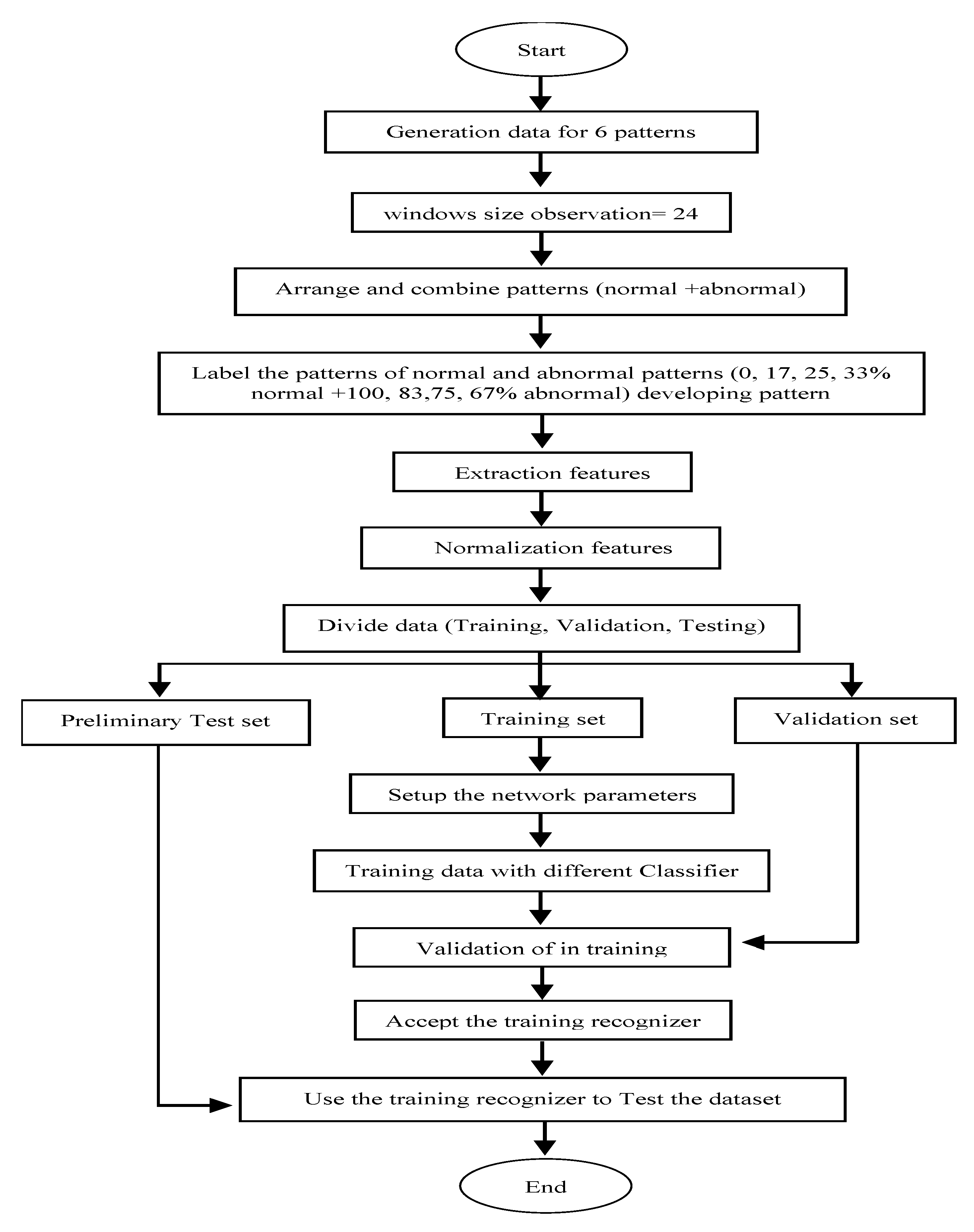
3.4. Results of Developing Patterns with Ensemble Classifier (Proposed Approach)

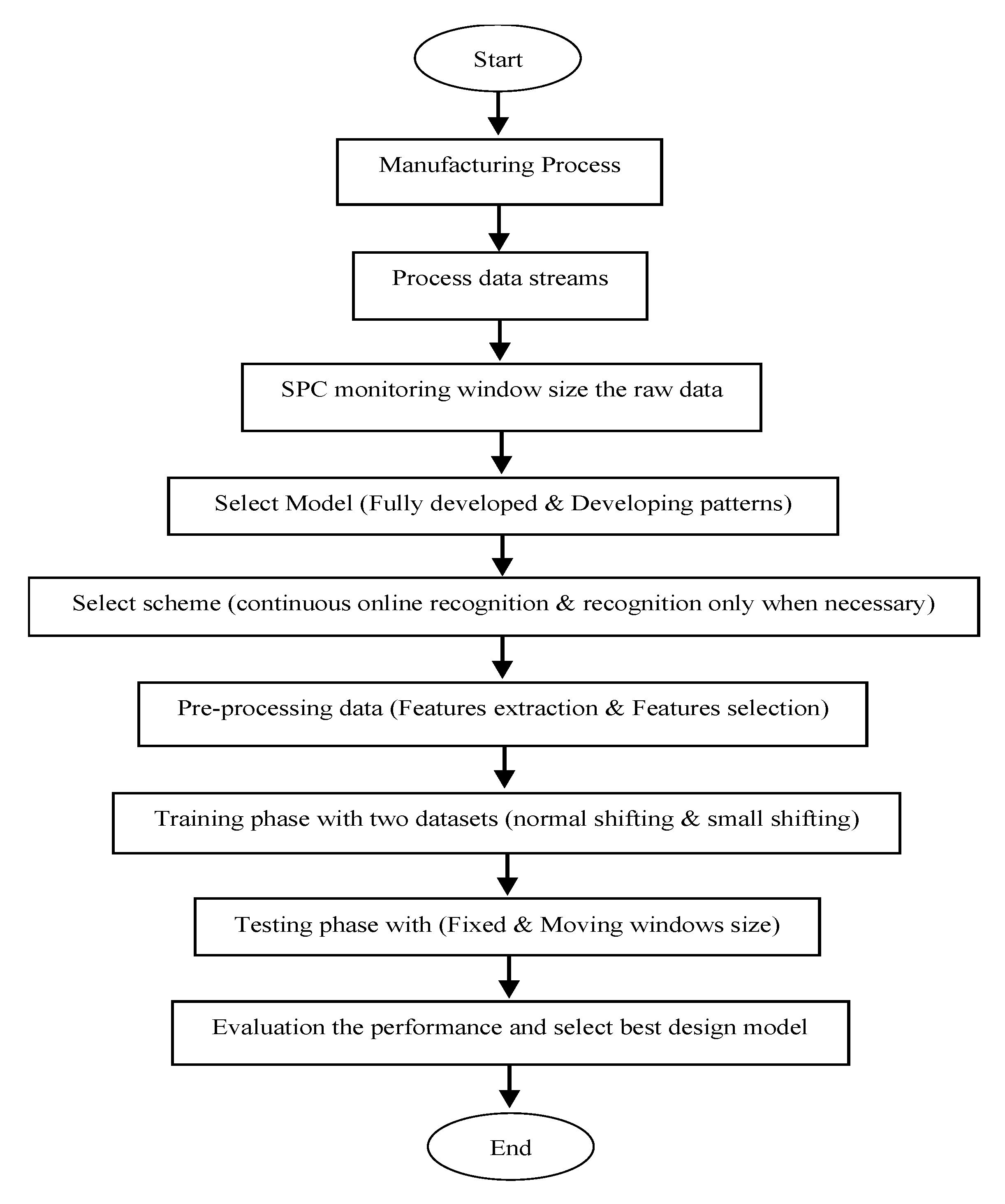
This study uses four different percentages of window size for abnormal patterns in the training data (100%, 83%, 75%, and 67%); each training dataset was evaluated to determine the optimal training data, which resulted in greater accuracy in the test phase.

• Case 1: Training data as 100% abnormal + 0% normal (0 normal point + 24 abnormal points) from point (31:54). In the first instance, this study identified the abnormal patterns in the same manner as in the prior case; all abnormal points were labeled as abnormal. As stated in

  Table 8. Percentage of abnormal pattern points in the labeling step.

  Normal	Abnormal
  30 points	30 points
  0%	100%

  , they were trained as full abnormal points from point 31 to point 60.

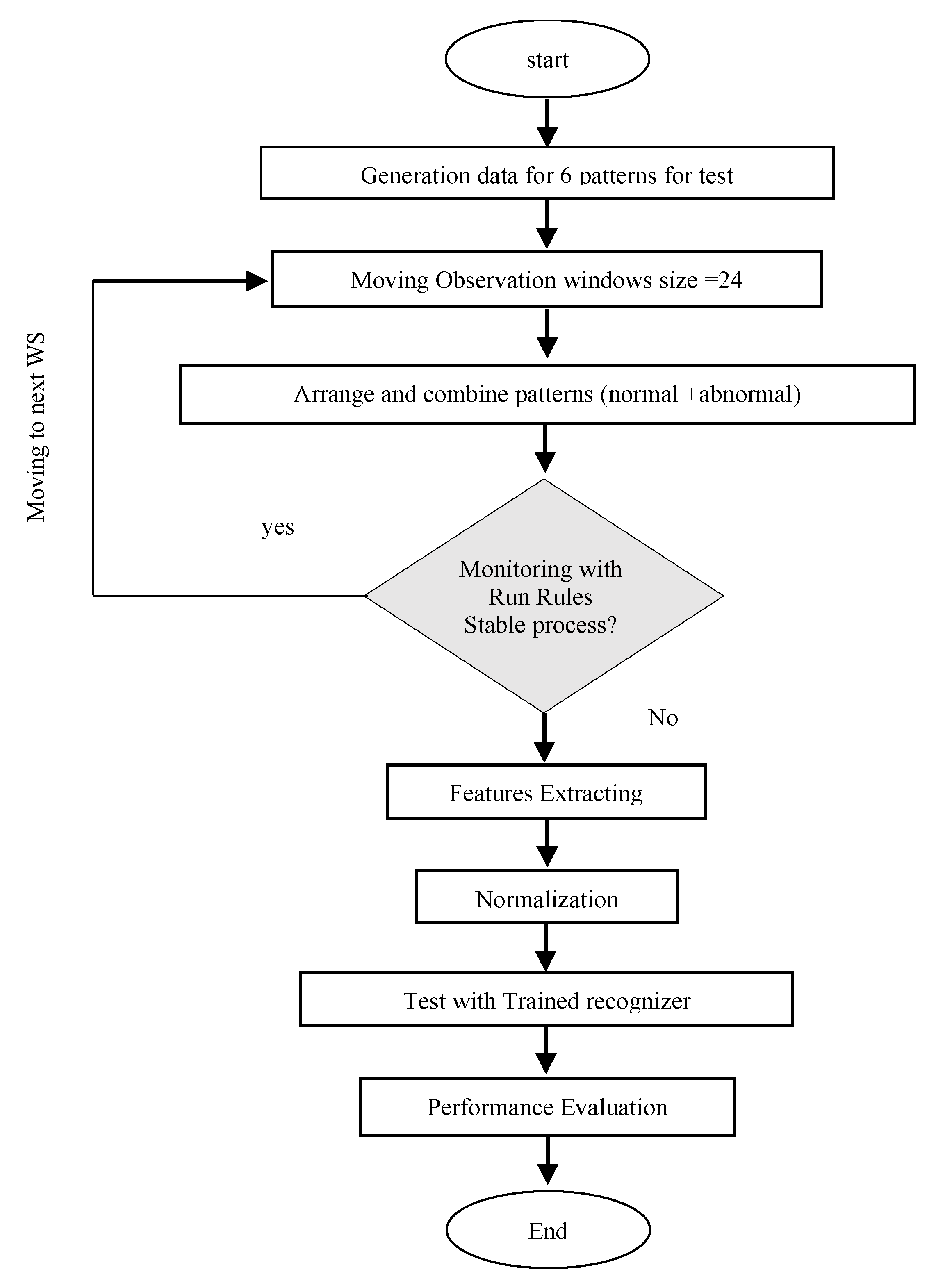
Six feature selections were used to apply the results of all the classification algorithms. This study compared two datasets, normal shift and small shift. All classifiers had acceptable identification accuracy for detecting a normal pattern (stable process), as observed. This benefit was implemented during the process of monitoring the run rules.

In the normal range for the mean shift dataset, the decision tree classifier had only 71% accuracy in spotting abnormal patterns for the cycle pattern. For the increasing trend, only 21% of inaccurate recognitions were correct, compared to 40% for normal and 39% for cycle. The poor accuracy on the downward trend was just 6%, compared to 59% for incorrect cycle recognition and 35% for normal recognition. For the increasing trend, the upper shift pattern yielded 87% correct recognition and 13% incorrect recognition. For the decreasing trend, the downshift pattern had 82% correct recognition and 18% incorrect recognition.

Table 9. Decision Tree Accuracy = 61.16%.

	NOR	CYC	IT	DT	US	DS
NOR	100	0	0	0	0	0
CYC	29	71	0	0	0	0
IT	40	39	21	0	0	0
DT	35	59	0	6	0	0
US	0	0	13	0	87	0
DS	0	0	0	18	0	82

shows that the overall rate of correct recognition is 61.16%. As demonstrated in

Table 10. ANN Accuracy = 81.50%.

	NOR	CYC	IT	DT	US	DS
NOR	95	3	0	2	0	0
CYC	4	96	0	0	0	0
IT	1	8	91	0	0	0
DT	61	0	0	39	0	0
US	0	0	23	0	77	0
DS	0	2	0	7	0	91

, the ANN classifier has 81.50% correct recognition. As indicated in

Table 11. Linear_SVM Accuracy = 95.16%.

	NOR	CYC	IT	DT	US	DS
NOR	100	0	0	0	0	0
CYC	12	88	0	0	0	0
IT	2	2	96	0	0	0
DT	7	3	0	90	0	0
US	0	0	1	0	99	0
DS	0	0	0	2	0	98

, the Linear Support Vector Machine classifier has a correct identification rate of 95.16%. As demonstrated in

Table 12. Gaussian_SVM Accuracy = 97.5%.

	NOR	CYC	IT	DT	US	DS
NOR	100	0	0	0	0	0
CYC	2	97	1	0	0	0
IT	3	0	97	0	0	0
DT	1	0	0	99	0	0
US	0	0	1	0	99	0
DS	0	0	0	7	0	93

, the Gaussian Support Vector machine classifier has a 97.5% correct identification rate. According to

Table 13. KNN_5 Accuracy = 91.83%.

	NOR	CYC	IT	DT	US	DS
NOR	99	1	0	0	0	0
CYC	13	87	0	0	0	0
IT	6	0	94	0	0	0
DT	0	0	0	100	0	0
US	0	0	17	0	83	0
DS	0	0	0	12	0	88

, the KNN-5 classifier has an accurate identification rate of 91.83%. As indicated in

Table 14. Ensemble Accuracy = 99.55%.

	NOR	CYC	IT	DT	US	DS
NOR	99.99	0.01	0	0	0	0
CYC	0.49	99.51	0	0	0	0
IT	0	0.46	99.54	0	0	0
DT	0	0.45	0	99.45	0	0
US	0	0	0.8	0	99.19	0
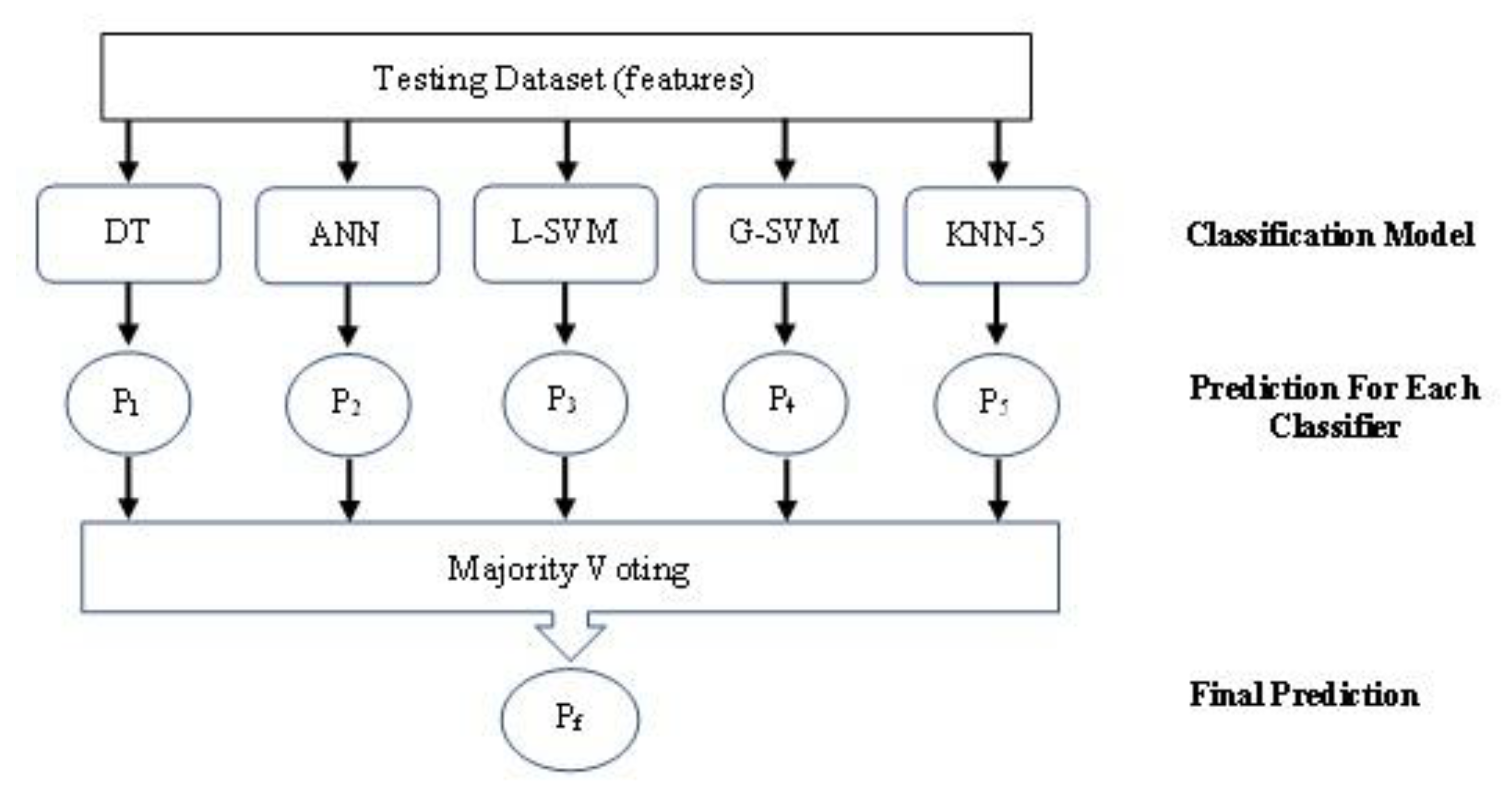
DS	0	0	0	0.3	0	99.66

, when the ensemble principle with majority voting was applied to these five distinct classifiers, decision-making improved, achieving a 99.55% accuracy level for each pattern.

For the small range mean shift dataset, this study indicates that all classifiers detect a normal pattern (stable process) with high identification accuracy. The accuracy of the decision tree classifier in detecting abnormal patterns for cycle pattern recognition is 100%. For the increasing trend, only 25% of respondents correctly identified it, while 68% misidentified it as an upper shift and 7% as a cycle. In addition, 57% of inaccurate recognitions were as a downshift, 14% of incorrect recognitions were as a cycle, and 5% were as normal, contributing to the low accuracy of the downward trend, which stands at just 24%. The normal and cycle recognition rates for the upwards shift pattern are 12% accurate recognition and 68% and 20% wrong recognition, respectively. In addition, the recognition rate for the downshift pattern is 7% correct, 73% incorrect as normal, and 20% incorrect as cycle. The correct recognition rate is 44.50% overall, as indicated in

Table 15. Decision Tree Accuracy = 44.50%.

	NOR	CYC	IT	DT	US	DS
NOR	99	1	0	0	0	0
CYC	0	100	0	0	0	0
IT	0	7	25	0	68	0
DT	5	14	0	24	0	57
US	68	20	0	0	12	0
DS	73	20	0	0	0	7

. According to

Table 16. ANN Accuracy = 84.16%.

	NOR	CYC	IT	DT	US	DS
NOR	100	0	0	0	0	0
CYC	35	65	0	0	0	0
IT	0	1	83	0	16	0
DT	0	0	0	69	0	31
US	0	12	0	0	88	0
DS	0	0	0	0	0	100

, the ANN classifier has an 84.16% correct recognition rate. According to

Table 17. Linear_SVM Accuracy = 92%.

	NOR	CYC	IT	DT	US	DS
NOR	100	0	0	0	0	0
CYC	21	79	0	0	0	0
IT	0	0	98	0	2	0
DT	1	0	0	86	0	13
US	3	1	0	0	96	0
DS	7	0	0	0	0	93

, the Linear Support Vector Machine classifier has a 92% correct recognition rate. According to

Table 18. Gaussian_SVM Accuracy = 93.83%.

	NOR	CYC	IT	DT	US	DS
NOR	100	0	0	0	0	0
CYC	1	93	0	0	0	0
IT	0	0	83	0	17	0
DT	0	0	0	100	0	0
US	0	0	0	0	100	0
DS	12	0	0	1	0	87

, the Gaussian Support Vector machine classifier has a correct identification rate of 93.83%. According to

Table 19. KNN_5 Accuracy = 91.83%.

	NOR	CYC	IT	DT	US	DS
NOR	99	1	0	0	0	0
CYC	4	91	0	0	5	0
IT	0	0	94	0	6	0
DT	0	0	0	98	0	2
US	14	1	3	0	82	0
DS	6	1	0	8	0	85

, the KNN-5 classifier has an accurate identification rate of 91.83%. As indicated in

Table 20. Ensemble Accuracy = 99.14%.

	NOR	CYC	IT	DT	US	DS
NOR	99.89	0	0	0	0.19	0
CYC	0.7	99.32	0	0	0	0
IT	0	0	99.27	0	0	0.7
DT	0	0	0	99.15	0	0.8
US	0	0	0.15	0	98.5	0
DS	0	0	0	1.2	0	98.7

, the ensemble principle with majority voting was applied to the five distinct classifiers, resulting in improved decision-making; a 99.14% accuracy level was achieved for each pattern.

In addition to calculating the ARL1 for each classifier, the results permit a comparison between the normal and small shift datasets. This study identifies superior accuracy of the five Gaussian Support Vector Machine classifiers for normal and small shifts, with 97.5 and 93.83%, respectively. On the other hand, the decision tree classifier is only able to achieve accuracy of 61.32 and 44.50%, respectively, on the normal and small shift databases. The respective ensemble recognition accuracy for the two datasets is 99.55 and 99.14%. This implies that several classifiers are superior to a single classifier as the first phase (ANN-MLP classifier) in the first model (Fully developed patterns), as the decision-making process is dependent on multiple classifiers. In addition, the accuracy increased when the run rules were implemented, from 99.05% and 98.37% for the normal shift and small shift, respectively, in the first model to 99.55% and 99.14% in the second model.

Table 21. Correct recognition and ARL1 for all of the classifiers.

Classifier	Normal Shifting (1.5–2.8) Sigma				Small Shifting (Less than (1.5) Sigma
	Training Accuracy%	Testing Accuracy Full Developed	Testing Accuracy Moving WS	ARL1	Training Accuracy%	Testing Accuracy Full Developed	Testing Accuracy Moving WS	ARL1
DT	99.51	98.32	61.16	13.35	99.44	97.47	44.50	13.58
ANN	99.07	99.01	81.5	13.65	98.74	98.46	84.16	13.91
L_SVM	99.02	99.07	95.16	14.05	98.28	98.10	92	14.14
G-SVM	99.05	99.01	97.5	13.83	98.35	98.30	93.83	13.94
KNN5	99.17	98.83	91.83	14.08	98.55	98.11	91.5	14.24
Ensemble	99.15	99.05	99.55	13.13	98.65	98.37	99.14	13.96

shows that the ARL1 improves from 14.34 to 13.96 with the new strategy utilized in the training phase.

• Case 2: In this instance, the size of the window is divided into training data as 83% abnormal + 17% normal (4 nor + 20 abnormal) from point (27:50). This study categorized 83% of the abnormal patterns during the window size (24 points) as abnormal and 17% as normal in this instance. As indicated in

  Table 22. Percentage of abnormal pattern points in the labeling step.

  Normal	Abnormal
  26 points	34 points
  17%	83%

  , all abnormal patterns (20 points abnormal versus 4 points normal) have been categorized as abnormal.

On the normal shift dataset, it is evident that the ensemble classifier has a 100% recognition accuracy for identifying normal patterns (stable process). This benefit is implemented during the run rules monitoring process. The accuracy of the decision tree classifier in spotting abnormal patterns for cycle pattern proper recognition is 96%, while it incorrectly labels just 3% as normal and 1% as an increasing trend. The increasing trend has a correct recognition rate of 66%; when incorrect, it identifies 32% as a cycle and 2% as normal. The accuracy of the decreasing trend is only 55% accurate, with 41% inaccurately recognized as normal and 4% as a cycle. As an ascending pattern, the upper shift pattern has a correct identification rate of 69% and an inaccurate recognition rate of 31%. In addition, 69% of those who recognize the downshift pattern correctly and 31% incorrectly do so as a decreasing trend. The decision tree has been enhanced from Case 1. As indicated in

Table 23. Decision Tree Accuracy = 75.83%.

	NOR	CYC	IT	DT	US	DS
NOR	100	0	0	0	0	0
CYC	3	96	1	0	0	0
IT	2	32	66	0	0	0
DT	41	4	0	55	0	0
US	0	0	31	0	69	0
DS	0	0	0	31	0	69

, the correct recognition rate was 75.83%, compared to 61.16% in Case 1. According to

Table 24. ANN Accuracy = 75.16%.

	NOR	CYC	IT	DT	US	DS
NOR	100	0	0	0	0	0
CYC	60	39	1	0	0	0
IT	7	0	93	0	0	0
DT	17	2	0	81	0	0
US	0	0	11	0	89	0
DS	0	0	0	51	0	49

, the ANN classifier has 75.16% correct recognition. As demonstrated in

Table 25. Linear_SVM Accuracy = 91%.

	NOR	CYC	IT	DT	US	DS
NOR	100	0	0	0	0	0
CYC	2	96	0	0	0	0
IT	6	0	94	0	0	0
DT	9	0	0	91	0	0
US	0	0	12	0	88	0
DS	0	0	0	23	0	77

, the Linear Support Vector Machine classifier has 91% accurate recognition. As indicated in

Table 26. Gaussian_SVM Accuracy = 93.83%.

	NOR	CYC	IT	DT	US	DS
NOR	100	0	0	0	0	0
CYC	1	98	0	1	0	0
IT	12	0	88	0	0	0
DT	2	0	0	98	0	0
US	0	0	5	0	95	0
DS	0	0	0	3	0	97

, the Gaussian Support Vector machine classifier has a correct identification rate of 93.83%. The KNN-5 classifier has 90.33% correct recognition, as shown in

Table 27. KNN_5 Accuracy = 90.33%.

	NOR	CYC	IT	DT	US	DS
NOR	100	0	0	0	0	0
CYC	16	82	2	0	0	0
IT	6	0	94	0	0	0
DT	1	1	0	98	0	0
US	0	0	25	0	75	0
DS	0	0	0	7	0	93

. The ensemble classifier has higher accuracy, achieving 99.07%, as shown in

Table 28. Ensemble Accuracy = 99.07%.

	NOR	CYC	IT	DT	US	DS
NOR	100	0	0	0	0	0
CYC	0	100	0	0	0	0
IT	0	0	98.3	0	0	1.6
DT	0	0	0	99.24	0	0.7
US	1.2	0	0	0	98.7	0
DS	0	0	0	1.7	0	98.2

.

For the small shift dataset, the decision tree classifier recognizes abnormal patterns for cycle pattern recognition with high accuracy. The increasing trend has 66% correct recognition in Case 2, compared to 25% in Case 1; 28% are incorrectly identified as a cycle and 6% as an upward shift. The recognition accuracy for the decreasing trend pattern is 64%, while it was only 24% in Case 1; 30% recognize it as a downshift, while 57% incorrectly identified it as a downshift in Case 1. With only 4% correct recognition for downshift and 86% incorrect recognition as cycle pattern, 6% as IT, and 4% as normal, the upper shift pattern has a low degree of accuracy. The downshift pattern has an identification rate of 21% correct, 74% incorrect as normal, 3% as a cycle, and 2% as a decreasing trend. The overall correct recognition rate is 59%, while in Case 1 it was 44.50%, as shown in

Table 29. Decision Tree Accuracy = 59%.

	NOR	CYC	IT	DT	US	DS
NOR	99	1	0	0	0	0
CYC	0	100	0	0	0	0
IT	0	28	66	0	6	0
DT	6	0	0	64	0	30
US	4	86	6	0	4	0
DS	74	3	0	2	0	21

. The ANN classifier has 81.33% correct recognition, as shown in

Table 30. ANN Accuracy = 81.33%.

	NOR	CYC	IT	DT	US	DS
NOR	100	0	0	0	0	0
CYC	5	95	0	0	0	0
IT	1	0	56	0	43	0
DT	1	0	0	96	0	0
US	1	9	0	0	90	0
DS	48	0	0	1	0	51

. However, the Linear Support Vector Machine classifier has 90.66% correct recognition, as shown in

Table 31. Linear_SVM Accuracy = 90.66%.

	NOR	CYC	IT	DT	US	DS
NOR	100	0	0	0	0	0
CYC	12	83	0	0	5	0
IT	0	0	74	0	26	0
DT	0	0	0	87	0	13
US	0	0	0	0	100	0
DS	0	0	0	0	0	100

. As indicated in

Table 32. Gaussian_SVM Accuracy = 93.83%.

	NOR	CYC	IT	DT	US	DS
NOR	100	0	0	0	0	0
CYC	6	89	1	0	4	0
IT	0	0	97	0	3	0
DT	0	0	0	95	0	5
US	2	0	3	0	95	0
DS	0	0	0	1	0	99

, the Gaussian Support Vector machine classifier has a correct identification rate of 93.83%, which is the same as in Case 1 irrespective of the training data used. According to

Table 33. KNN_5 Accuracy = 80.83%.

	NOR	CYC	IT	DT	US	DS
NOR	100	0	0	0	0	0
CYC	12	82	3	0	2	1
IT	0	0	81	0	19	0
DT	0	0	0	77	0	23
US	8	0	35	0	57	0
DS	6	0	0	6	0	88

, the KNN-5 classifier has an accurate identification rate of 80.83%. As demonstrated in

Table 34. Ensemble Accuracy = 98.2%.

	NOR	CYC	IT	DT	US	DS
NOR	100	0	0	0	0	0
CYC	0	98.5	0	0	1.4	0
IT	2.2	0	97.7	0	0	0
DT	0	0	0	98.4	0	1.6
US	1.7	0	2.1	0	96.1	0
DS	0	0	0	1.7	0	98.2

, the ensemble classifier achieves a higher accuracy of 98.2% for each pattern.

For normal and small shifts, the accuracy of these five classifiers in the Gaussian Support Vector Machine classifier is 96% and 95.83%, respectively, compared to 97.5% and 93.83% in Case 1. The decision tree classifier improved from 61.32% and 44.50% for normal and small shifts in Case 1 to 75.83% and 59%, respectively. On both datasets, the ensemble classifier has a correct recognition rate of 99.07% and 98.2%, respectively. As shown in

Table 35. Correct recognition and ARL1 for all the classifiers.

Classifier	Normal Shifting (1.5–2.8) Sigma				Small Shifting (Less than (1.5) Sigma
	Training Accuracy%	Testing Accuracy Full Developed	Testing Accuracy Moving WS	ARL1	Training Accuracy%	Testing Accuracy Full Developed	Testing Accuracy Moving WS	ARL1
DT	98.60	94.58	75.83	13.32	97.75	90.40	59	15.13
ANN	96.78	96.22	75.16	13.02	93.24	92.75	81.33	13.34
L_SVM	96.11	95.72	91	12.16	92.76	92.58	90.66	12.87
G_SVM	96.42	95.90	96	12.35	93.26	92.86	95.83	13.11
KNN5	97.20	96.04	90.33	12.69	94.84	92.05	80.83	13.16
Ensemble	98.82	96.14	99.07	12.63	98.54	92.90	98.2	13.09

, with the ensemble classifier the ARL1 improved in Case 2 compared to Case 1, from 13.13 and 13.96 to 12.63 and 13.09 for the normal and small shift databases, respectively.

• Case 3: Data collected during training were interpreted as follows: 75% abnormal and 25% normal (6 nor + 18 abnormal) from point (25:48). In this case, the abnormal patterns that occurred within the window size of 24 points were labeled as 75% abnormal and 25% normal. This indicates that the study categorized all of the abnormal patterns (18 points classified as abnormal and 6 points classified as normal) and labeled them as abnormal, as indicated in

  Table 36. The percentage of abnormal pattern points in the labeling step.

  Normal	Abnormal
  24 points	36 points
  25%	75%

  .

The accuracy of the decision tree classifier in recognizing abnormal patterns for cycle pattern accurate recognition is high at 82%, and it incorrectly labels only 14% as normal and 4% as an increasing trend. The IT pattern has 92% correct recognition, compared to 66% in Case 2, 7% incorrect recognition as cycle, compared to 32% in Case 2, and 1% as normal. The poor recognition rate for the DT pattern is just 66%, compared to 55% for Case 2; 33% of incorrect identifications are as normal and only 1% as cycle. The recognition rate for the upwards shift pattern is 74%, compared to 69% in Case 2, and 26% of incorrect recognitions are as an IT. In addition, the DS pattern has 85% correct recognition, compared to 69% in Case 2. Moreover, 15% of incorrect recognitions are as a DT pattern. The decision tree is improved from Case 2. The overall correct recognition is 83.16%, when it was 75.83% in Case 2, as shown in

Table 37. Decision Tree Accuracy = 83.16%.

	NOR	CYC	IT	DT	US	DS
NOR	100	0	0	0	0	0
CYC	14	82	4	0	0	0
IT	1	7	92	0	0	0
DT	33	1	0	66	0	0
US	0	0	26	0	74	0
DS	0	0	0	15	0	85

. The ANN classifier has 73.50% correct recognition, as shown in

Table 38. ANN Accuracy = 73.50%.

	NOR	CYC	IT	DT	US	DS
NOR	98	0	0	2	0	0
CYC	3	80	8	9	0	0
IT	2	0	98	0	0	0
DT	44	0	0	56	0	0
US	0	0	14	0	86	0
DS	0	4	0	73	0	23

. The Linear Support Vector Machine classifier has 81.16% correct recognition, as shown in

Table 39. Linear_SVM Accuracy = 81.16%.

	NOR	CYC	IT	DT	US	DS
NOR	100	0	0	0	0	0
CYC	18	81	1	0	0	0
IT	17	0	83	0	0	0
DT	8	0	0	92	0	0
US	0	0	27	0	73	0
DS	0	0	0	42	0	58

. The Gaussian Support Vector machine classifier has 94.50% correct recognition, an improvement from Case 2 at 93.83%, as shown in

Table 40. Gaussian_SVM Accuracy = 94.50%.

	NOR	CYC	IT	DT	US	DS
NOR	100	0	0	0	0	0
CYC	3	96	1	0	0	0
IT	14	0	86	0	0	0
DT	9	0	0	91	0	0
US	0	0	4	0	96	0
DS	0	0	0	2	0	98

. The KNN-5 classifier improves from Case 2 as well, from 90.33% to 92.50% correct recognition, as shown in

Table 41. KNN_5 Accuracy = 92.50%.

	NOR	CYC	IT	DT	US	DS
NOR	100	0	0	0	0	0
CYC	5	95	0	0	0	0
IT	9	0	91	0	0	0
DT	2	0	0	98	0	0
US	0	0	19	0	81	0
DS	0	0	0	10	0	90

. Finally, the Ensemble classifier has higher accuracy at 98%, as shown in

Table 42. Ensemble Accuracy = 98%.

	NOR	CYC	IT	DT	US	DS
NOR	100	0	0	0	0	0
CYC	0	97.3	0	0	2.7	0
IT	1.7	0	98.22	0	0	0
DT	0	0	0	98.1	0	1.89
US	0	0	3.8	0	96.17	0
DS	1.3	0	0	0	0	98.61

.

The decision tree classifier has a high level of accuracy when it comes to recognizing abnormal patterns for the small shift dataset, with a correct recognition rate of 97% for the cycle pattern and a rate of 3% for incorrect detection as normal. For an increased trend, correct recognition is at 62%, while incorrect recognition is at 28% as a cycle pattern, and normal recognition is at 2%. The accuracy of identifying a decreasing trend increased to 87% from 64% in Case 1, with 4% of incorrect recognitions as a cycle, and 2% as normal. For the upwards shift pattern, the correct recognition accuracy increases to 49% from 4% in Case 2, while the incorrect recognition rate decreases to 27% as a cycle pattern, 22% as an increasing trend, and 2% as normal. The downshift pattern is improved as well, from 21% correct recognition in Case 2 to 35%, with 62% of incorrect recognitions being as a decreasing trend, 2% as normal, and 1% as cycle. Previously, it had a correct recognition of just 21% in Case 2. As can be seen in

Table 43. Decision Tree Accuracy = 71.66%.

	NOR	CYC	IT	DT	US	DS
NOR	100	0	0	0	0	0
CYC	3	97	0	0	0	0
IT	2	28	62	0	8	0
DT	2	4	0	87	0	7
US	2	27	22	0	49	0
DS	2	1	0	62	0	35

, the total correct recognition is 71.66, when in Case 2 it was equal to 59% and in Case 1 to 44.50%. According to

Table 44. ANN Accuracy = 77.66%.

	NOR	CYC	IT	DT	US	DS
NOR	100	0	0	0	0	0
CYC	5	95	0	0	0	0
IT	14	3	65	0	18	0
DT	11	0	0	87	0	2
US	4	9	21	0	66	0
DS	25	0	0	22	0	53

, the ANN classifier has a recognition accuracy rate of 77.66%.

Table 45. Linear_SVM Accuracy = 71.83%.

	NOR	CYC	IT	DT	US	DS
NOR	100	0	0	0	0	0
CYC	16	78	0	0	5	1
IT	1	0	31	0	68	0
DT	1	0	0	23	0	76
US	0	0	1	0	99	0
DS	0	0	0	0	0	100

reveals that the Linear Support Vector Machine classifier achieves a recognition accuracy of 71.83%. According to

Table 46. Gaussian_SVM Accuracy = 83.33%.

	NOR	CYC	IT	DT	US	DS
NOR	100	0	0	0	0	0
CYC	8	87	4	0	1	0
IT	5	0	87	0	8	0
DT	3	0	0	44	0	53
US	0	0	16	0	84	0
DS	0	0	0	2	0	98

, the Gaussian Support Vector machine classifier has a correct recognition rate of 83.33%. According to

Table 47. KNN_5 Accuracy = 82.33%.

	NOR	CYC	IT	DT	US	DS
NOR	100	0	0	0	0	0
CYC	7	88	2	0	2	1
IT	1	0	93	0	6	0
DT	10	0	0	89	0	1
US	8	0	36	0	56	0
DS	0	3	0	29	0	68

, the KNN-5 classifier improves from an incorrect recognition rate of 80.83% in Case 2 to a rate of 82.33%. According to the data presented in

Table 48. Ensemble Accuracy = 97.95%.

	NOR	CYC	IT	DT	US	DS
NOR	100	0	0	0	0	0
CYC	2	97	0	0	1	0
IT	0	0	98.42	0	0	1.3
DT	1.39	0	0	98.61	0	0
US	0	0	4	0	95.97	0
DS	0.2	0	0	2	0	97.71

, the ensemble classifier achieves a high accuracy of 97.95%.

Additionally, the ARL1 for each classifier is calculated. The greater accuracy of these five classifiers in the Gaussian Support Vector Machine classifier is 94% for the normal shift database and 92.05% for the small shift database. The respective normal and small shift classification increases from 75.83% and 59% in Case 2 to 83.16 and 71.66. For both datasets, the ensemble classifier achieves 97.95% correct recognition. With the ensemble classifier, the ARL1 improves in Case 3 compared to Case 2, as shown in

Table 49. Correct recognition and ARL1 for all the classifiers.

Classifier	Normal Shifting (1.5–2.8) Sigma				Small Shifting (Less than (1.5) Sigma
	Training Accuracy%	Testing Accuracy Full Developed	Testing Accuracy Moving WS	ARL1	Training Accuracy%	Testing Accuracy Full Developed	Testing Accuracy Moving WS	ARL1
DT	98.61	94.27	83.16	12.87	97.58	90.47	71.66	13.05
ANN	96.38	95.88	73.50	12.02	92.84	91.91	77.66	12.97
L_SVM	95.65	95.51	81.16	11.25	92.08	91.19	71.83	11.78
G-SVM	96.08	95.95	94.50	12.09	92.70	92.05	83.33	12.52
KNN5	97.03	95.69	92.5	12.24	94.70	91.73	82.33	12.86
Ensemble	98.27	96.15	98	12.04	97.53	92.15	97.95	12.52

, from 12.63 and 13.09 to 12.04 and 12.52 for the normal and small shift databases, respectively.

• Case 4: Training data as 67% abnormal + 33% normal (8 normal points + 16 abnormal points) from point (23:46). In this case, the study labeled the abnormal patterns during the window size (24 points) as 67% abnormal and 33% normal. That means that the study labeled all abnormal patterns (16 points abnormal with 8 points normal) and labeled them as abnormal patterns during labeling, as shown in

  Table 50. The percentage of abnormal pattern points in the labeling step.

  Normal	Abnormal
  22 points	38 points
  33%	67%

  .

For the normal shift dataset, it is clear that all the classifiers have recognition accuracy of 100% when detecting a normal pattern (stable process). The decision tree classifier has good recognition accuracy for abnormal patterns, with a cycle pattern correct recognition rate of 75%; when wrong, it classifies 20%as normal and 5% as an IT pattern. The increasing trend pattern has 64% correct recognition, and for incorrect recognitions 32% are as a cycle and 4% as normal. The accuracy in the DT pattern is poor, with just 51% correct recognition; 48% of incorrect recognitions are as normal and 1% as a cycle. The upwards shift pattern improves from 74% correct recognition in Case 3 to 82%, and all 18% of incorrect recognitions are as an increasing trend. Likewise, the downward shift pattern has 82% correct recognition, with 17% of incorrect recognitions as a decreasing trend and 1% as normal. The overall correct recognition is 75.66%, as shown in

Table 51. Decision Tree Accuracy = 75.66%.

	NOR	CYC	IT	DT	US	DS
NOR	100	0	0	0	0	0
CYC	20	75	5	0	0	0
IT	4	32	64	0	0	0
DT	48	1	0	51	0	0
US	0	0	18	0	82	0
DS	0	1	0	17	0	82

. The ANN classifier improves from 73.50% correct recognition in Case 3 to 86.33%, as shown in

Table 52. ANN Accuracy = 86.33%.

	NOR	CYC	IT	DT	US	DS
NOR	99	1	0	0	0	0
CYC	1	98	1	9	0	0
IT	3	2	95	0	0	0
DT	12	4	0	84	0	0
US	0	0	19	0	81	0
DS	0	0	0	39	0	61

. The Linear Support Vector Machine classifier achieves 79% correct recognition, as shown in

Table 53. Linear_SVM Accuracy = 79%.

	NOR	CYC	IT	DT	US	DS
NOR	100	0	0	0	0	0
CYC	10	88	2	0	0	0
IT	14	0	86	0	0	0
DT	10	0	0	90	0	0
US	0	0	37	0	63	0
DS	0	0	0	53	0	47

. The Gaussian Support Vector machine classifier has 95.16% correct recognition, improving from 94.50% in Case 3 and 93.83% in Case 2, as shown in

Table 54. Gaussian_SVM Accuracy = 95.16%.

	NOR	CYC	IT	DT	US	DS
NOR	100	0	0	0	0	0
CYC	3	96	1	0	0	0
IT	9	0	91	0	0	0
DT	6	0	0	94	0	0
US	0	0	4	0	96	0
DS	0	0	0	6	0	98

. The KNN-5 classifier has 88% correct recognition, as shown in

Table 55. KNN_5 Accuracy = 88%.

	NOR	CYC	IT	DT	US	DS
NOR	100	0	0	0	0	0
CYC	8	89	2	1	0	0
IT	9	1	90	0	0	0
DT	13	0	0	87	0	0
US	0	0	23	0	77	0
DS	0	0	0	15	0	85

. the ensemble classifier achieves a high accuracy of 98.32%, as shown in

Table 56. Ensemble Accuracy = 98.32%.

	NOR	CYC	IT	DT	US	DS
NOR	100	0	0	0	0	0
CYC	0	98.1	0	0	1.8	0
IT	0.18	0	99.8	0	0	0
DT	0	0	0	98.63	0	1.3
US	1.2	0	2.4	0	96.4	0
DS	0	0	0	2.99	0	97.01

.

For the small shift dataset, the decision tree classifier has good accuracy in recognizing the abnormal patterns for cycle patterns, with correct recognition of 94%; of incorrect recognitions, 3% are as an increasing trend and 3% as normal. For increasing trend patterns, recognition improves from 62% in Case 3 to 76%, with 10% of incorrect recognitions as normal, 7% as cycle patterns, and 7% as upwards shifts. The accuracy of the DT pattern is 74%. Moreover, 18% of incorrect recognitions are as normal, 7% as downshifts, and 1% as cycles. The upwards shift pattern has 47% correct recognition, with 47% of incorrect recognitions as an increasing trend, 5% as a cycle pattern, and 1% as normal. The downshift pattern improves from 35% correct recognition in Case 3 to 56%, with 34% of incorrect recognitions as a decreasing trend, 7% as a cycle, and 3% as normal. The overall correct recognition is 74.50%; in Case 3 it was 71.66%, in Case 2 it was 59%, and in Case 1 it was 44.50%, as shown in

Table 57. Decision Tree Accuracy = 74.50%.

	NOR	CYC	IT	DT	US	DS
NOR	100	0	0	0	0	0
CYC	3	94	3	0	0	0
IT	10	7	76	0	7	0
DT	18	1	0	74	0	7
US	1	5	47	0	47	0
DS	3	7	0	34	0	56

. The ANN classifier improves from 77.66% correct recognition in Case 3 to 85%, as shown in

Table 58. ANN Accuracy = 85%.

	NOR	CYC	IT	DT	US	DS
NOR	100	0	0	0	0	0
CYC	4	96	0	0	0	0
IT	10	1	68	0	21	0
DT	0	0	0	91	0	9
US	3	4	3	0	90	0
DS	2	0	0	33	0	65

. The Linear Support Vector Machine classifier has 67.5% correct recognition, as shown in

Table 59. Linear_SVM Accuracy = 67.50%.

	NOR	CYC	IT	DT	US	DS
NOR	100	0	0	0	0	0
CYC	10	82	0	0	7	1
IT	11	0	17	0	72	0
DT	4	0	0	19	0	77
US	1	0	3	0	96	0
DS	0	0	0	9	0	91

. The Gaussian Support Vector machine classifier improves from 83.33% correct recognition in Case 3 to 85.66%, as shown in

Table 60. Gaussian_SVM Accuracy = 85.66%.

	NOR	CYC	IT	DT	US	DS
NOR	100	0	0	0	0	0
CYC	5	86	2	0	6	1
IT	4	0	92	0	4	0
DT	7	0	0	87	0	6
US	1	0	25	0	74	0
DS	0	0	0	25	0	75

. The KNN-5 classifier has 97% correct recognition, as shown in

Table 61. KNN_5 Accuracy = 79%.

	NOR	CYC	IT	DT	US	DS
NOR	100	0	0	0	0	0
CYC	10	85	2	0	1	2
IT	2	0	89	0	9	0
DT	5	0	0	90	0	5
US	1	2	44	0	53	0
DS	4	0	0	39	0	57

. The ensemble classifier achieves high accuracy of 97.03% for each pattern, as shown in

Table 62. Ensemble Accuracy = 97.03%.

	NOR	CYC	IT	DT	US	DS
NOR	100	0	0	0	0	0
CYC	3.5	96.59	0	0	0	0
IT	0	0	95.9	0	4	0
DT	0	0	0	98.98	0	1.02
US	0	0	4.2	0	95.71	0
DS	1.8	0	0	3	0	95

.

The highest accuracy of these five classifiers is the Gaussian Support Vector machine classifier, with 95.16% and 85.66% for the normal and small shift datasets, respectively. The ensemble accuracy is 98.32% and 97.03% correct recognition for the normal and small shift ranges, respectively. The ARL1 is improved in Case 4 compared to Case 3, from 12.04 and 12.52 to 11.65 and 11.94 for the normal and small shift databases, respectively, with the results for the ensemble classifier shown in

Table 63. Correct recognition and ARL1 for all the classifiers.

Classifier	Normal Shifting (1.5–2.8) Sigma				Small Shifting (Less than (1.5) Sigma
	Training Accuracy%	Testing Accuracy Full Developed	Testing Accuracy Moving WS	ARL1	Training Accuracy%	Testing Accuracy Full Developed	Testing Accuracy Moving WS	ARL1
DT	98.37	94.06	75.66	11.72	97.17	89.30	74.5	12.30
ANN	95.78	95.52	86.33	11.38	91.50	91.42	85	11.89
L_SVM	94.51	94.80	79	11.09	89.97	90.57	67.5	11.21
G-SVM	95.27	95.40	95.16	12.07	90.81	91.49	85.66	12.19
KNN5	96.53	95.26	88	11.94	94.02	91.14	79	12.31
Ensemble	98.59	95.70	98.32	11.65	98.02	91.84	97.03	11.94

.

The current study is compared with, Lu, Wang [2], who proposed an approach with dynamic observation window sizes (OWS) to study the different cutting parameters, implementing four different classifier algorithms. The shift range in their study was just (1.5–2.5 sigma), a different range than that in the present study, which used a normal shift range of (1.5–2.8 sigma) and small shift range of less than (1.5 sigma) with five different classifier algorithms and an ensemble classifier.

We note here that it is very clear that the previous study has a drawback with normal pattern recognition, as the present work achieves 98.32% recognition on all pattern classes with the ensemble classifier. The maximum recognition accuracy for the previous work, with Gaussian-SVM, is 95.6%, while this study the same classifier achieves 95.16%. However, the ensemble classifier has 98.32% recognition accuracy. The comparison of this study with [2] for a normal shift range is shown in

Table 64. Comparison of the present work with Lu [2].

Classifier	This Work		Lu, Wang [2]
	Training Accuracy%	Testing Accuracy Moving WS	Training Accuracy%			Testing Accuracy%
			Normal Condition	Abnormal Condition	Average	Normal Condition	Abnormal Condition	Average
DT	98.37	75.66	100	100	100	67.2	98.4	82.8
ANN	95.78	86.33	99.1	99.5	99.3	63.5	99.1	81.3
L_SVM	94.51	79	----	----	----	----	----	---
G-SVM	95.27	95.16	100	100	100	71.4	98.9	85.15
KNN-5	96.53	88	98	99.6	98.8	59.2	98.1	78.8
Ensemble	98.59	98.32	----	----	----	----	-----	---

.

In detail, they combined their two OWS for improved recognition accuracy. The highest recognition accuracy they were able to reach with Gaussian-SVM was 95.6%. This study investigated four cases for different training datasets with five different classifier algorithms and ensemble classifiers with (MV) techniques. The highest recognition accuracy is 99.55%, achieved with the ensemble classifier, as shown in

Table 65. Four cases in the present study versus two OWS in [2].

Classifier	This Work				Lu, Wang [2]
Widows Size	Case1	Case2	Case3	Case4	OWS1	OWS2	OWS1+OWS2
DT	61.1	75.9	83.2	75.7	85.2	88.7	93.4
ANN	81.5	75.1	73.5	86.3	86.8	89.5	91.7
L_SVM	95.1	91	81.2	79	----	----	----
G-SVM	97.5	96	94.5	95.2	87.2	84.9	95.6
KNN-5	91.8	90.3	92.5	88	82.8	83.9	89.9
Ensemble	99.6	98.7	98	98.3	----	----	----

.

This approach was compared to others used in earlier studies to recognize control chart patterns with small change variation. The results of the present study indicate that the ensemble classifier has greater recognition accuracy in CCPR, attaining 99.55% and 99.14%, respectively, when using a normal shift range and a small shift range.

4. Discussion

The classification that was produced by the ensemble classifier was more accurate than the classifications produced by the individual classifiers. The decision-making of the ensemble classifier is the result of a collaborative effort made by five different classifiers, with the vote of the majority of classifiers serving as the final decision. We discovered that the proportion of incorrect answers for the final decision dropped. The purpose of this study was to classify abnormal patterns with a mean shift less than 1.5 sigma by analysing small shifts. This process replicates the online growth of a process through the use of moveable windows. It can recognize abnormal patterns as soon as is feasible, reducing production waste if at all possible. The purpose of the four training scenarios was to decrease the average run length for the abnormal patterns (ARL1). The run rules differentiate between normal and abnormal patterns, contributing to the improvement of the model and the reduction of misclassification. The similarities and differences between this study and previous research are presented in

Table 66. Comparison of this work with previous works.

Ref.	Model	Learning Algorithm	Optimization	Input	No. of Patterns	%
[29]	KELM	MGWO	kernel entropy component analysis KECA as a feature reduction algorithm	feature fusion extraction (FFE)	6 Basic + 4 mixes	99.5
[21]	MLP	scaled conjugate gradient algorithm (SCG)	Bees’ algorithm (BA) to find the best features	shape features	6	99.5
[53]	MLP	resilient back-propagation	EWMA computation the incomplete data	Statistical features	6	99.2
[31]	RBF	Bees’ algorithm	association rules (AR)	Statistical & shape features	8	99.36
[25]	MLP	Levenberg-Marquardt (LM)	a hybrid system based on statistical and shape features and multi-layer perceptrons neural network (MLPNN)	Statistical & shape features	8	99.5
[24]	MLP	Back-propagation (BP)	Recognition patterns in bivariate SPC	Statistical features	Nain Category	96
[67]	MLP	descending gradient algorithm	new feature belief variable	Statistical features	6	97.36
[68]	MLP	Levenberg-Marquardt (LM) algorithm	One feature with three values	Statistical features	5	100
[20]	MLP	Levenberg-Marquardt (LM)	cuckoo optimization algorithm (COA)	Shape features	6	99.21
[69]	RBF	Back-propagation (BP)	bee’s algorithm (BA)	Shape features	6	99.61
[70]	MLP	descending gradient algorithm	MEWMA-ANNs	Statistical features	8	86.57
[71]	MLP	Levenberg-Marquardt (LM)	One feature with three values	Statistical features	5	100
[72]	MLP	Back-propagation (BP)	two-stage intelligent monitoring scheme (2S-IMS)	Statistical features	7	98.5
[73]	MLP	BP	(ICA) for the separation step and a decision tree	Shape features	6 basic + 6 mixed	87.96
[38]	MLP	Levenberg– Marquardt (LM)	--------	Statistical & shape features	6	99.15
[39]	MLP	BFGS	new feature extraction method without defining the basic patterns	pattern displacement into account	7	98.05
[74]	MLP	RBF	PSO	Euclidean distance	6	99.26
[40]	MLP	ABP	improvement of the training algorithm	Statistical & shape features	6	99.21
This work	MLP	Levenberg-Marquardt (LM)	New feature selection approach (RCF)	Statistical & shape features	6	99.05
This work	Ensemble		New feature selection approach (RCF)	Statistical & shape features	6	99.55

.

The ensemble classifier significantly improves recognition accuracy (99.55%), as seen in Table 66. This demonstrates that the performance of the ensemble classifier is superior to that of the individual classifiers for the normal shift range. Within a small variation range, the ensemble approach achieved 99.14% recognition accuracy. The run rules utilized in this article demonstrate that the classification of both datasets (small and normal) is nearly flawless (100%) for a stable process.

5. Conclusions

This study presents an improved control chart pattern recognition (CCPR) model focusing on small mean shifts for X-bar chart patterns. We began with the commonly utilized ANN-MLP algorithm from previous CCPR experiments. The MLP classifier achieved a classification accuracy of 98.88% for normal mean shifting and 98.13% for small mean shifting. Our study revealed that the recognition accuracy is enhanced when implementing an ensemble of five classifiers, namely, decision tree, ANN, linear support vector machine, Gaussian support vector machine, and KNN-5. The ensemble classifier reached an improved recognition accuracy of 99.55% for mean shifting within (±3σ) and 99.14% for small mean shifting within (±1.5σ). We observed that the ARL1 was reduced from 15.5 to 11.94 for small mean shifting, suggesting that the implemented ensemble classifier enables faster and more accurate detection. This study is a step forward in the intelligence manufacturing domain. It provides production and quality managers a tool for addressing process variability, particularly within small changes in the process mean. It can provide a useful guide for quality engineers in developing and implementing automated CCPR systems. This research can be extended in the future to investigate multivariate patterns, as well as other pattern classes.

References

1. Zaman, M.; Hassan, A. Improved statistical features-based control chart patterns recognition using ANFIS with fuzzy clustering. Neural Comput. Appl. 2019, 31, 5935–5949. [Google Scholar] [CrossRef]
2. Lu, Z.; Wang, M.; Dai, W. A condition monitoring approach for machining process based on control chart pattern recognition with dynamically-sized observation windows. Comput. Ind. Eng. 2020, 142, 106360. [Google Scholar] [CrossRef]
3. Testik, M.C.; Kara, O.; Knoth, S. An algorithmic approach to outlier detection and parameter estimation in Phase I for designing Phase II EWMA control chart. Comput. Ind. Eng. 2020, 144, 106440. [Google Scholar] [CrossRef]
4. Atalay, M.; Caner Testik, M.; Duran, S.; Weiß, C.H. Guidelines for automating Phase I of control charts by considering effects on Phase-II performance of individuals control chart. Qual. Eng. 2020, 32, 223–243. [Google Scholar] [CrossRef]
5. Saleh, N.A.; Mahmoud, M.A.; Keefe, M.J.; Woodall, W.H. The difficulty in designing Shewhart X and X control charts with estimated parameters. J. Qual. Technol. 2015, 47, 127–138. [Google Scholar] [CrossRef]
6. Ebrahimzadeh, A.; Ranaee, V. Control chart pattern recognition using an optimized neural network and efficient features. ISA Trans. 2010, 49, 387–393. [Google Scholar] [CrossRef]
7. Lin, S.Y.; Guh, R.S.; Shiue, Y.R. Effective recognition of control chart patterns in autocorrelated data using a support vector machine based approach. Comput. Ind. Eng. 2011, 61, 1123–1134. [Google Scholar] [CrossRef]
8. Bag, M.; Gauri, S.K.; Chakraborty, S. Feature-based decision rules for control charts pattern recognition: A comparison between CART and QUEST algorithm. Int. J. Ind. Eng. Comput. 2012, 3, 199–210. [Google Scholar] [CrossRef]
9. Wu, C.; Liu, F.; Zhu, B. Control chart pattern recognition using an integrated model based on binary-tree support vector machine. Int. J. Prod. Res. 2015, 53, 2026–2040. [Google Scholar] [CrossRef]
10. Cuentas, S.; Peñabaena-Niebles, R.; Garcia, E. Support vector machine in statistical process monitoring: A methodological and analytical review. Int. J. Adv. Manuf. Technol. 2017, 91, 485–500. [Google Scholar] [CrossRef]
11. Al-Ghanim, A.; Jordan, J. Automated process monitoring using statistical pattern recognition techniques on X-bar control charts. J. Qual. Maint. Eng. 1996, 2, 25–49. [Google Scholar] [CrossRef]
12. Hassan, A.; Baksh, M.S.N.; Shaharoun, A.M.; Jamaluddin, H. Improved SPC chart pattern recognition using statistical features. Int. J. Prod. Res. 2003, 41, 1587–1603. [Google Scholar] [CrossRef]
13. Du, S.; Huang, D.; Lv, J. Recognition of concurrent control chart patterns using wavelet transform decomposition and multiclass support vector machines. Comput. Ind. Eng. 2013, 66, 683–695. [Google Scholar] [CrossRef]
14. Gauri, S.K.; Chakraborty, S. Feature-based recognition of control chart patterns. Comput. Ind. Eng. 2006, 51, 726–742. [Google Scholar] [CrossRef]
15. Gauri, S.K.; Chakraborty, S. Recognition of control chart patterns using improved selection of features. Comput. Ind. Eng. 2009, 56, 1577–1588. [Google Scholar] [CrossRef]
16. Kim, J.-M.; Wang, N.; Liu, Y.; Park, K. Residual Control Chart for Binary Response with Multicollinearity Covariates by Neural Network Model. Symmetry 2020, 12, 381. [Google Scholar] [CrossRef] [Green Version]
17. Yu, J.; Zheng, X.; Wang, S. A deep autoencoder feature learning method for process pattern recognition. J. Process Control 2019, 79, 1–15. [Google Scholar] [CrossRef]
18. Haghighati, R.; Hassan, A. Feature extraction in control chart patterns with missing data. In Proceedings of the International Conference on Mechanical and Manufacturing Engineering (ICME2018), Johor, Malaysia, 16–17 July 2018; p. 012013. [Google Scholar]
19. Bag, M.; Gauri, S.K.; Chakraborty, S. An expert system for control chart pattern recognition. Int. J. Adv. Manuf. Technol. 2012, 62, 291–301. [Google Scholar] [CrossRef]
20. Addeh, A.; Maghsoudi, B.M. Control chart patterns detection using COA based trained MLP neural network and shape features. Comput. Res. Prog. Appl. Sci. Eng. 2016, 2, 5–8. [Google Scholar]
21. Wong, P.; Chua, A. Control chart pattern identification using a synergy between neural networks and bees algorithm. Ann. Electr. Electron. Eng. 2019, 2, 8–13. [Google Scholar] [CrossRef]
22. Wani, M.A.; Rashid, S. Parallel algorithm for control chart pattern recognition. In Proceedings of the Fourth International Conference on Machine Learning and Applications (ICMLA′05), Los Angeles, CA, USA, 15–17 December 2005; p. 5. [Google Scholar]
23. Imani, M.; Montazer, G.A. A survey of emotion recognition methods with emphasis on E-Learning environments. J. Netw. Comput. Appl. 2019, 147, 102423. [Google Scholar] [CrossRef]
24. Sohaimi, N.; Masood, I.; Md Nor, D. Bivariate SPC Chart Pattern Recognition Using Modular-Neural Network. In Proceedings of the International PostGraduate Conference on Applied Science & Physics 2017, Johor, Malaysia, 7 December 2017. [Google Scholar]
25. Addeh, A.; Zarbakhsh, P.; Seyedzadeh Kharazi, S.J.; Harastani, M. A Hierarchical System for Recognition of Control Chart Patterns. In Proceedings of the 2018 International Conference on Advances in Computing and Communication Engineering, ICACCE, Paris, France, 22–23 June 2018; pp. 423–427. [Google Scholar]
26. Votto, R.; Ho, L.L.; Berssaneti, F. Multivariate control charts using earned value and earned duration management observations to monitor project performance. Comput. Ind. Eng. 2020, 148, 106691. [Google Scholar] [CrossRef]
27. Aziz Kalteh, A.; Babouei, S. Control chart patterns recognition using ANFIS with new training algorithm and intelligent utilization of shape and statistical features. ISA Trans. 2020, 102, 12–22. [Google Scholar] [CrossRef] [PubMed]
28. Zhang, M.; Yuan, Y.; Wang, R.; Cheng, W. Recognition of mixture control chart patterns based on fusion feature reduction and fireworks algorithm-optimized MSVM. Pattern Anal. Appl. 2020, 23, 15–26. [Google Scholar] [CrossRef]
29. Zhang, M.; Zhang, X.; Wang, H.; Xiong, G.; Cheng, W. Features Fusion Exaction and KELM with Modified Grey Wolf Optimizer for Mixture Control Chart Patterns Recognition. IEEE Access 2020, 8, 42469–42480. [Google Scholar] [CrossRef]
30. Zhao, C.; Wang, C.; Hua, L.; Liu, X.; Zhang, Y.; Hu, H. Recognition of Control Chart Pattern Using Improved Supervised Locally Linear Embedding and Support Vector Machine. Procedia Eng. 2017, 174, 281–288. [Google Scholar] [CrossRef]
31. Addeh, A.; Khormali, A.; Golilarz, N.A. Control chart pattern recognition using RBF neural network with new training algorithm and practical features. ISA Trans. 2018, 79, 202–216. [Google Scholar] [CrossRef]
32. Pelegrina, G.D.; Duarte, L.T.; Jutten, C. Blind source separation and feature extraction in concurrent control charts pattern recognition: Novel analyses and a comparison of different methods. Comput. Ind. Eng. 2016, 92, 105–114. [Google Scholar] [CrossRef] [Green Version]
33. Khajehzadeh, A.; Asady, M. Recognition of control chart patterns using adaptive neuro-fuzzy inference system and efficient features. Int J Sci Eng Res 2015, 6, 771–779. [Google Scholar]
34. Zhang, M.; Cheng, W. Recognition of Mixture Control Chart Pattern Using Multiclass Support Vector Machine and Genetic Algorithm Based on Statistical and Shape Features. Math. Probl. Eng. 2015, 2015, 382395. [Google Scholar] [CrossRef] [Green Version]
35. Addeh, J.; Ebrahimzadeh, A.; Azarbad, M.; Ranaee, V. Statistical process control using optimized neural networks: A case study. ISA Trans. 2014, 53, 1489–1499. [Google Scholar] [CrossRef] [PubMed]
36. Ebrahimzadeh, A.; Addeh, J.; Ranaee, V. Recognition of control chart patterns using an intelligent technique. Appl. Soft Comput. 2013, 13, 2970–2980. [Google Scholar] [CrossRef]
37. Addeh, J.; Ebrahimzadeh, A.; Nazaryan, H. A Research about Pattern Recognition of Control Chart Using Optimized ANFIS and Selected Features. J. Eng. Technol. 2013, 3, 6. [Google Scholar] [CrossRef]
38. Ranaee, V.; Ebrahimzadeh, A. Control chart pattern recognition using neural networks and efficient features: A comparative study. Pattern Anal. Appl. 2013, 16, 321–332. [Google Scholar] [CrossRef]
39. Cheng, C.S.; Huang, K.K.; Chen, P.W. Recognition of control chart patterns using a neural network-based pattern recognizer with features extracted from correlation analysis. Pattern Anal. Appl. 2012, 18, 75–86. [Google Scholar] [CrossRef]
40. Addeh, J.; Ebrahimzadeh, A.; Ranaee, V. Control chart pattern recognition using adaptive back-propagation artificial Neural networks and efficient features. In Proceedings of the 2011 2nd International Conference on Control, Instrumentation and Automation, ICCIA 2011, Shiraz, Iran, 27–29 December 2011; pp. 742–746. [Google Scholar]
41. Ranaee, V.; Ebrahimzadeh, A.; Ghaderi, R. Application of the PSO–SVM model for recognition of control chart patterns. ISA Trans. 2010, 49, 577–586. [Google Scholar] [CrossRef]
42. Zorriassatine, F.; Tannock, J.; O′Brien, C. Using novelty detection to identify abnormalities caused by mean shifts in bivariate processes. Comput. Ind. Eng. 2003, 44, 385–408. [Google Scholar] [CrossRef]
43. Yu, J.; Xi, L.; Zhou, X. Identifying source(s) of out-of-control signals in multivariate manufacturing processes using selective neural network ensemble. Eng. Appl. Artif. Intell. 2009, 22, 141–152. [Google Scholar] [CrossRef]
44. Al-Assaf, Y. Recognition of control chart patterns using multi-resolution wavelets analysis and neural networks☆. Comput. Ind. Eng. 2004, 47, 17–29. [Google Scholar] [CrossRef]
45. Liu, X.; He, S.; Gu, Y.; Xu, Z.; Zhang, Z.; Wang, W.; Liu, P. A robust cutting pattern recognition method for shearer based on Least Square Support Vector Machine equipped with Chaos Modified Particle Swarm Optimization and Online Correcting Strategy. ISA Trans. 2020, 99, 199–209. [Google Scholar] [CrossRef]
46. Kontonatsios, G.; Spencer, S.; Matthew, P.; Korkontzelos, I. Using a neural network-based feature extraction method to facilitate citation screening for systematic reviews. Expert Syst. Appl. X 2020, 6, 100030. [Google Scholar] [CrossRef]
47. Smith, A.E. X-bar and R control chart interpretation using neural computing. Int. J. Prod. Res. 1994, 32, 309–320. [Google Scholar] [CrossRef]
48. Hassan, A. Ensemble ANN-based recognizers to improve classification of X-bar control chart patterns. In Proceedings of the 2008 IEEE International Conference on Industrial Engineering and Engineering Management, Singapore, 8–11 December 2008; pp. 1996–2000. [Google Scholar]
49. Pandya, A.S.; Macy, R.B. Pattern Recognition with Neural Networks in C++; CRC Press: Boca Raton, FL, USA, 1995. [Google Scholar]
50. Simon, H. Neural Networks: A Comprehensive Foundation; Prentice Hall: Hoboken, NJ, USA, 1999. [Google Scholar]
51. Pham, D.; Oztemel, E. Control chart pattern recognition using combinations of multi-layer perceptrons and learning-vector-quantization neural networks. Proc. Inst. Mech. Eng. Part I J. Syst. Control Eng. 1993, 207, 113–118. [Google Scholar] [CrossRef]
52. Zaman, M.; Hassan, A. Fuzzy heuristics and decision tree for classification of statistical feature-based control chart patterns. Symmetry 2021, 13, 110. [Google Scholar] [CrossRef]
53. Haghighati, R.; Hassan, A. Recognition performance of imputed control chart patterns using exponentially weighted moving average. Eur. J. Ind. Eng. 2018, 12, 637–660. [Google Scholar] [CrossRef]
54. Russo, R.; Romano, G.; Colombo, P. Identification of various control chart patterns using support vector machine and wavelet analysis. Ann. Electr. Electron. Eng. 2019, 2, 6–12. [Google Scholar]
55. Xu-Dong, X.; Li-Qian, M. Control Chart Recognition Method Based on Transfer Learning. In Proceedings of the 2018 4th Annual International Conference on Network and Information Systems for Computers, ICNISC 2018, Wuhan, China, 19–21 April 2018; pp. 446–451. [Google Scholar]
56. Hong, Z.; Li, Y.; Zeng, Z. Convolutional neural network for control chart patterns recognition. In Proceedings of the ACM International Conference Proceeding Series, Sanya, China, 22–24 October 2019. [Google Scholar]
57. Zan, T.; Su, Z.; Liu, Z.; Chen, D.; Wang, M.; Gao, X. Pattern Recognition of Different Window Size Control Charts Based on Convolutional Neural Network and Information Fusion. Symmetry 2020, 12, 1472. [Google Scholar] [CrossRef]
58. Alwan, W.; Hassan, A.; Ngadiman, N.H.A. A Review on Input Features for Control Chart Patterns Recognition. In Proceedings of the 11th Annual International Conference on Industrial Engineering and Operations Management, Singapore, 7–11 March 2021. [Google Scholar]
59. Randhawa, K.; Loo, C.K.; Seera, M.; Lim, C.P.; Nandi, A.K. Credit card fraud detection using AdaBoost and majority voting. IEEE Access 2018, 6, 14277–14284. [Google Scholar] [CrossRef]
60. Hassan, A. An improved scheme for online recognition of control chart patterns. Int. J. Comput. Aided Eng. Technol. 2011, 3, 309–321. [Google Scholar] [CrossRef]
61. Zaman, M.; Hassan, A. X-barControl Chart Patterns Identification Using Nelson’s Run Rules. In Proceedings of the 11th Annual International Conference on Industrial Engineering and Operations Management, Singapore, 7–11 March 2021. [Google Scholar]
62. Masood, I.; Hassan, A. A Scheme for Balanced Monitoring and Accurate Diagnosis of Bivariate Process Mean Shifts. Ph.D. Thesis, Universiti Teknologi Malaysia, Johor Bahru, Malaysia, 2012. [Google Scholar]
63. Tsai, C.-F. Combining cluster analysis with classifier ensembles to predict financial distress. Inf. Fusion 2014, 16, 46–58. [Google Scholar] [CrossRef]
64. Sharkey, A.; Nets, C.A.N. Ensemble and Modular Multi-Net Systems. Comb. Artif. Neural Nets 1999, 1, 1–25. [Google Scholar]
65. West, D.; Dellana, S.; Qian, J. Neural network ensemble strategies for financial decision applications. Comput. Oper. Res. 2005, 32, 2543–2559. [Google Scholar] [CrossRef]
66. Kittler, J.; Hatef, M.; Duin, R.P.; Matas, J. On combining classifiers. IEEE Trans. Pattern Anal. Mach. Intell. 1998, 20, 226–239. [Google Scholar] [CrossRef] [Green Version]
67. Bayati, N. Pattern recognition in control chart using neural network based on a new statistical feature. Int. J. Eng. 2017, 30, 1372–1380. [Google Scholar]
68. Rahman, N.A.; Masood, I.; Rahman, M.N.A.; Nasir, N.F. Control chart pattern recognition in metal stamping process using statistical features-ANN. J. Telecommun. Electron. Comput. Eng. 2017, 9, 5–9. [Google Scholar]
69. Addeh, A. Control Chart Pattern Recognition Using Associated Rules and Optimized Classifier. Comput. Res. Prog. Appl. Sci. Eng. 2016, 2, 71–80. [Google Scholar]
70. Masood, I.; Shyen, V.B.E. Quality control in hard disc drive manufacturing using pattern recognition technique. In Proceedings of the International Engineering Research and Innovation Symposium (IRIS), Melaka, Malaysia, 24–25 November 2016. [Google Scholar]
71. Rahman, N.A.; Masood, I.; Rahman, M.N.A. Recognition of unnatural variation patterns in metal-stamping process using artificial neural network and statistical features. In Proceedings of the International Engineering Research and Innovation Symposium (IRIS), Melaka, Malaysia, 24–25 November 2016. [Google Scholar]
72. Masood, I.; Hassan, A. Bivariate quality control using two-stage intelligent monitoring scheme. Expert Syst. Appl. 2014, 41, 7579–7595. [Google Scholar] [CrossRef]
73. Chompu-Inwai, R.; Thaiupathump, T. Improved ICA-based mixture control chart patterns recognition using shape related features. In Proceedings of the 2015 IEEE Conference on Control and Applications, CCA 2015, Sydney, Australia, 21–23 September 2015; pp. 484–489. [Google Scholar]
74. Addeh, J.; Ebrahimzadeh, A.; Ranaee, V. Application of the PSO-RBFNN model for recognition of control chart patterns. In Proceedings of the 2011 2nd International Conference on Control, Instrumentation and Automation, ICCIA 2011, Shiraz, Iran, 27–29 December 2011; pp. 747–752. [Google Scholar]
Figure 1. Flowchart of the models using normal shift and small shift datasets.
Machines 11 00115 g001
Figure 2. Structure of an Ensemble Classifier with Majority Voting.
Machines 11 00115 g002
Figure 3. The training flowchart for the fully developed patterns model using normal shift and small shift datasets.
Machines 11 00115 g003
Figure 4. Testing flowchart for the fully developed patterns model using normal shift and small shift datasets.
Machines 11 00115 g004
Figure 5. The training flowchart for the developing patterns model using normal shift and small shift datasets.
Machines 11 00115 g005
Figure 6. Testing flowchart for the developing patterns model using normal shift and small shift datasets.
Machines 11 00115 g006