1. Introduction
Vibrations represent an intrinsic problem in all fields of mechanical engineering including rotordynamics. Rotating machines are subject to remarkable loads and, with the development of machines that operate above some critical speeds, the control of vibrations is fundamental to guarantee long time operation. The typical problems in this field are excessive steady state synchronous vibration levels and subsynchronous rotor instabilities. The first one usually arises from excessive unbalance or due to operation close to a critical speed. The second one may depend on the presence of instability sources, connected to cross-coupling effects present in bearing systems and seals, among others. In some cases, the increase of the vibration, when crossing a critical speed during a runup or a rundown, can be harmful for the operation of the machine and the addition of some damping to the system is often required.
To this aim, squeeze film dampers remain one of the most effective components used because they offer the advantage of dissipating vibration energy when the shaft is supported by rolling element bearings. In addition, SFDs can improve the dynamic stability characteristics of rotor-bearing systems.
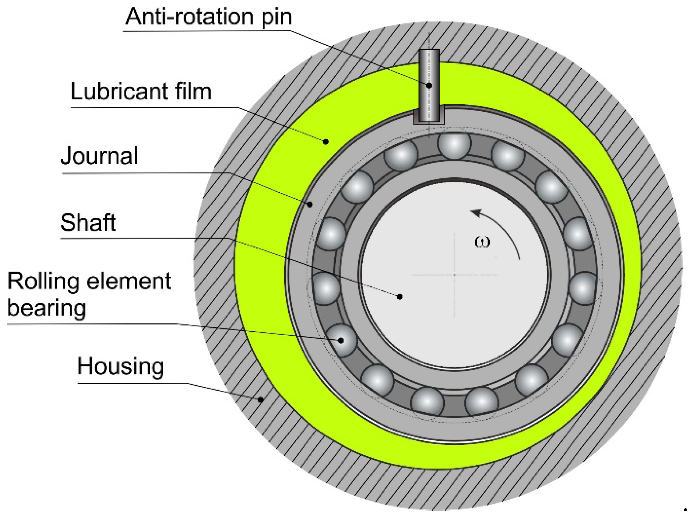
The most common design for these components is the one coupled with a rolling element bearing, as shown in
Figure 1.
The shaft is supported by a rolling element bearing and the coupling is often referenced as journal. The shaft vibration is transferred to the external ring of the bearing that “squeezes” the lubricant film, placed between the housing and the outer surface of the journal, generating high dynamic pressures. Therefore, dynamic forces counteract the lateral displacement of the shaft generating the damping effect. The anti-rotation pin is often applied to avoid any spinning motion of the journal, so that only translational displacements are possible, i.e., the journal can only translate or orbit without spinning about its axis of symmetry. The shaft spinning is decoupled from the journal motion thanks to the presence of the bearing.
This configuration is characterized by strong non-linearities due to the “bottoming-out”: the journal remains in contact with the casing surface at the run-up; when the level of the vibration is increased, the detachment of the two components happens resulting in a discontinuous change of the properties of the system. To reduce the non-linearity and the risk of collision between the static element and the whirling one in the case of large journal displacements, different supports are used, such as O-rings and squirrel cages. The selection of the proper stiffness of the support is fundamental for the correct operation of the SFD. If the support is too stiff, no relative motion between the shaft and the cage will be possible, i.e., no squeezing of the oil film; whereas if the stiffness is too low, the SFD can behave like a non-supported one [
1,
2].
Damping is the design parameter for all SFDs, and an optimal value for each application must be obtained. As a matter of fact, the utilization of a device whose damping capability is not aligned with the one requested by the system is useless if not dangerous. If the level of damping is too high, the SFD will dynamically behave as a rigid connection. Conversely, if the level of damping is too small, nothing will change in the dynamic response of the machine.
There are many studies in the literature that provide guidelines to determine the correct damping needed by a machine. In general, it depends on the dynamic characteristics of the machine itself, the typical operating conditions, and the kind of excitations [
3,
4].
Different models with different levels of complexity have been developed to predict the dynamic characteristics of SFDs. The first ones were based on the 1 D Reynolds equation for short plain journal bearings. This approximation is legitimate when the length to diameter ratio is lower than 0.25 and if no sealing mechanism is adopted, [
5]. The effect of the SFD on the journal is modeled by means of linearized stiffness and damping coefficients likewise oil-film bearings. If no spinning motion is considered, no stiffening effect is obtained from the SFD. On the contrary, the long bearing approximation can be adopted when the length to diameter ratio tends to infinity or if seals limiting the oil flow are applied. In both cases, an analytical solution is possible. For this reason, many estimations of the coefficients are present in the literature [
2,
3].
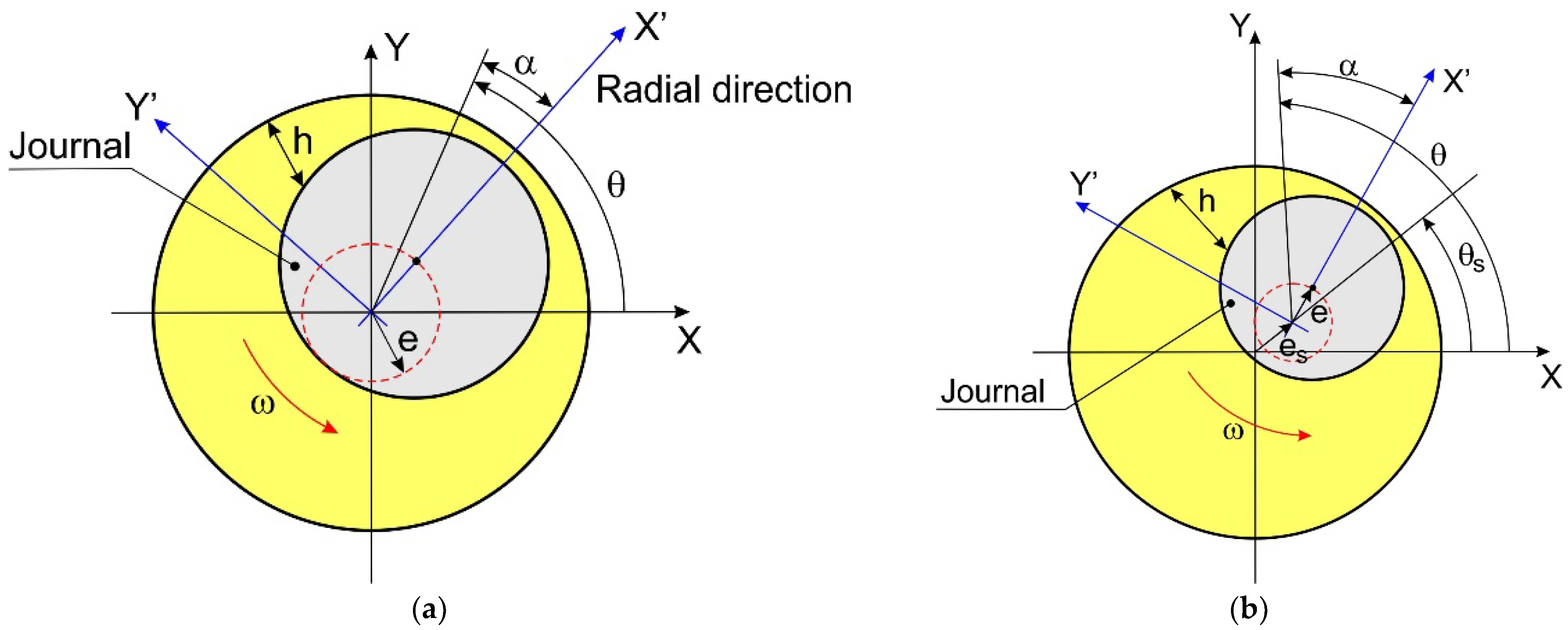
The motion of the shaft is modelled, for convenience, as i) circular synchronous precessions, centered or with a static eccentricity, or ii) small amplitude motions about a static displaced center. The first model is usually applied when the response to unbalance is investigated, the second one is used for critical speed and stability analyses as shown by San Andrés in [
6].
From these early works, it is possible to understand that the clearance and the length to diameter ratio are two important parameters influencing the operation of the bearing together with the amplitude of the vibration, [
1,
2,
3].
The 1-D Reynolds equation model has the advantage of simplicity, but the predictions can be considered reliable only for very simple geometries and for a limited range of operating conditions.
The main phenomena affecting the dynamic performance of SFDs are the fluid inertia, the liquid cavitation, the air ingestion, and the geometrical features.
Inertia is usually neglected in the derivation of the Reynolds equation, but for large clearances and amplitudes of motion, associated to higher vibrational frequencies, the added mass produced by the oil dynamic pressurization found experimentally has a value comparable to the mass of the entire SFD as highlighted by San Andrés and Vance in [
7]. Different models that consider the effect of inertia can be found in the literature. As also reported by San Andrés and Vance in [
8], for moderate values of the squeeze Reynolds number (
with
and
being the density and dynamic viscosity of the oil respectively,
the vibration frequency and
the SFD clearance) the fluid inertia can be assumed not to affect the shape of the fluid purely viscous velocity profiles and consider the fluid temporal inertia in the modeling of SFDs. In [
9], the effects of convective inertia and temporal inertia are considered together. In [
10], a detailed description of the equations necessary to include the inertial contribution is presented together with an application.
Cavitation is stated as one of the principal reasons why predictions on the force coefficients, made with the simple model used in [
1,
5], do not fit the experimental results. For this reason, relevant effort has been put in the investigation and modeling of cavitation. In [
11], Zeidan and Vance experimentally recognized five different cavitation regimes: un-cavitated film, cavitation bubble following the journal, oil–air mixture, vapor cavitation, vapor and gaseous cavitation. The second regime is considered as a transient condition, steady only for reduced whirling frequencies, that evolves in the third one with the shaft acceleration. The most common regimes are the third and fourth that sometimes combine with each other. Diaz and San Andrés in [
12] concentrated mostly on vapor cavitation and air entrainment. They tested a bearing in open-ends and in fully flooded configuration, changing whirling frequencies and pressure of supply oil, and measuring the dynamic pressure generated. The authors showed the difference between the pressure evolution in time for the two-cavitation mechanism. For the vapor cavitation, the pressure profile is nearly identical for every cycle, while for air entrainment the pressure measurements showed great variability from one cycle to the other. Similar conclusions regarding the gaseous cavitation can be found in [
13].
Due to the differences measured between the two phenomena, vapor cavitation and air ingestion are treated and modeled differently. Different vapor cavitation models and algorithms have been developed. The first cavitation model that was introduced is the so called
π-film model, also known as Gumbel condition. Here, the relative pressure is considered zero in the region where it assumes negative values. According to this hypothesis, the ruptured film extends over half the angular length of the bearing. One of the most used algorithms is the so-called Elrod’s cavitation algorithm, [
14]. An evolution of this approach consists in the adoption of the linear complementarity problem (LCP), [
15].
In [
8,
16,
17] the effect of air ingestion and bubbly mixture is experimentally investigated. Air is “sucked” inside the SFD, and, after some cycles, the bubbles of air are finely dispersed in the mixture and persist also in the high-pressure zone. The presence of a compressible foamy mixture can explain the variability of the pressure’s peak values. Different models that take into account the air ingestion are present in the literature. Among them, Diaz [
18] provided a detailed procedure, supported by a series of experimental results, to include the air ingestion effect in the 2D Reynolds equation, based on the hypothesis of a homogeneous bubbly mixture. To correctly determine the percentage of air inside of the mixture, a reference value is needed. In the experimental campaign, the air volume fraction is controlled at the feeding system. In industrial applications the SFD is fed with pure oil and air is ingested from the discharge locations. It is therefore necessary to predict the reference value of ingested air. In [
19], the authors introduced a model to evaluate the air entrainment in open-ends short SFDs. Some years later, Mendez et al. [
20] adapted Diaz’s model to finite length bearings. Both the models presented in [
18,
20] are based on a simplified form of the Rayleigh–Plesset equation to model the presence of air bubbles in the oil in open-ends SFDs. Gehannin et al. in [
21] considered instead the complete form of the equation and proposed a comparison with experimentally derived measures to evaluate the impact of these two different forms of the equation on the accuracy of the model.
Regarding the geometrical characteristics of the SFD, in [
22], San Andrés et al. reported an extensive experimental campaign that thoroughly investigates the effect of different geometrical features on the dynamic properties of the SFDs. Six different configurations are tested, and the focus is set on the effect on the force coefficients of film clearance, length of the SFD, groove feeding and hole feeding, sealing ends and open ends, whirl orbit amplitude, shape of orbit, and number and disposition of feed holes.
In this paper, a comprehensive model based on the 2D Reynolds equation is introduced: The different phenomena described above are taken into considerations and discussed. The model is then validated with experimental and numerical data taken from the literature. The modeling of the different phenomena describing the dynamic behavior of SFDs is taken from several past works found in the literature. A simplified approach is considered to reduce the level of the difficulty and the parameters to be controlled. The goal of this work is to obtain a model that can be easily replicated and adapted.
In the literature there are more refined models based on the bulk-flow equations [
23], and computational fluid dynamics [
24,
25,
26,
27]. Both approaches guarantee higher precision of the results, but the modeling and computational effort is higher than the one required by the model proposed in this work. The latter one gives the opportunity of investigating different phenomena in an approachable and straightforward way.
Eventually, an example of application of a SFD to a centrifugal compressor rotor for the reduction of vibration is proposed and a parametric investigation on the different parameters influencing the dynamic behavior of SFDs is performed. Moreover, the effect of the application of a SFD on the correction of an instability is also presented. In future works, the model proposed will be revised and improved to increase the accuracy.
3. Model Validation
The model was validated with both numerical and experimental data available in the literature. The numerical and experimental results presented in [
22] were considered due to the different geometrical configuration tested. In this work, four configurations (SFD A, B, E and F) were selected as reference for the validation. They differ in terms of clearance, SFD length, as well as the presence of a central groove and an end seal. The tested diameter is constant and equal to 127 mm. In [
22], the oil has density
and dynamic viscosity
. The geometrical characteristics of the SFDs considered for the validation are listed in
Table 1.
SFDs E and F are tested with a fixed static eccentricity and by changing the amplitude of the circular orbit vibration. The considered
ratios are:
,
,
and
. The tested frequencies are
for SFD E and
for SFD F. The obtained coefficients are constant for the whole frequency range, therefore only the values at
and 5
are shown respectively. The evolution of both the mass and damping coefficients for SFD F is shown in
Figure 7, where it is possible to see that the results obtained with the model presented in this paper agree well with both the experimental and numerical results in [
22].
Both the numerical results for the mass coefficient shown in
Figure 7a underestimate the experimental results. In [
22], the authors attribute the discrepancy to the high value of the feeding pressure that determines a higher value of the radial component of the force, directly responsible for the mass coefficient.
Similarly, the evolution of the mass and damping coefficient for SFD E is shown in
Figure 8. In this case only the experimental results are available. It is possible to notice an acceptable agreement for the damping coefficients, the maximum difference between the experimental and numerical results is lower than the 25%. On the other hand, an important discrepancy between for the mass coefficients is shown. A possible explanation could be the high level of the feeding pressure that strongly affects the dynamic pressure distribution.
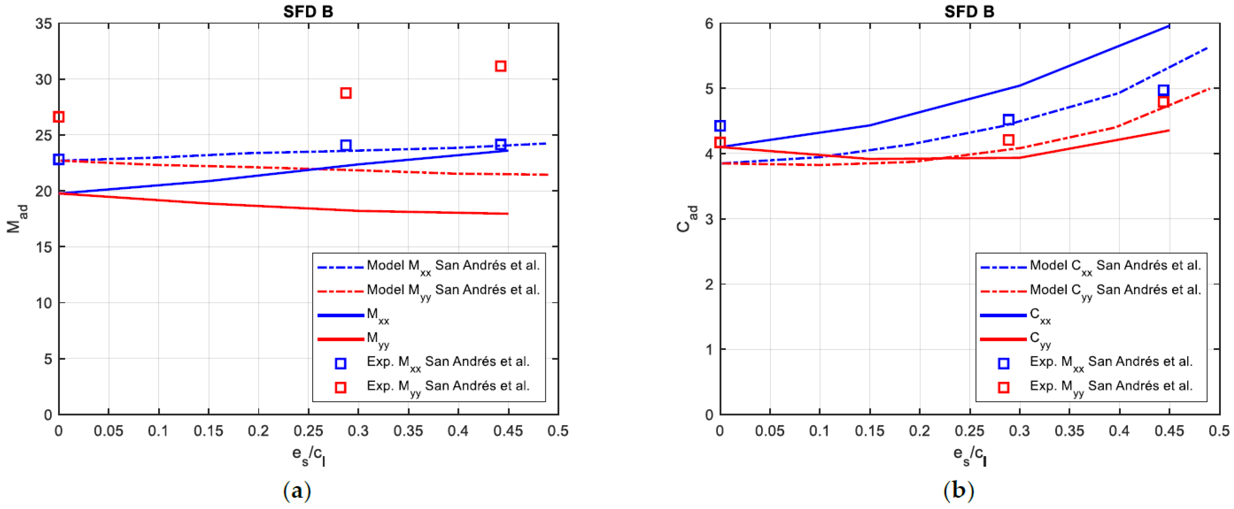
SFDs B and A are tested in [
22] at different static eccentricities with a constant orbit radius
and for the frequency range
. Moreover, for these configurations, there is no variation of the force coefficients with the frequency and the only frequency considered is
. For both configurations, the effective groove depth is tuned to match the results presented in [
22]. The evolution of the dynamic coefficients with the static eccentricity for the open-ends configuration of SFD B is shown in
Figure 9. Similarly to SFD F, the numerical results agree well with the experimental ones. A similar trend was obtained for SFD A. The results are not reported for the sake of brevity. In
Figure 9, the values of the force coefficients are adimensionalized considering the same reference values reported in [
22].
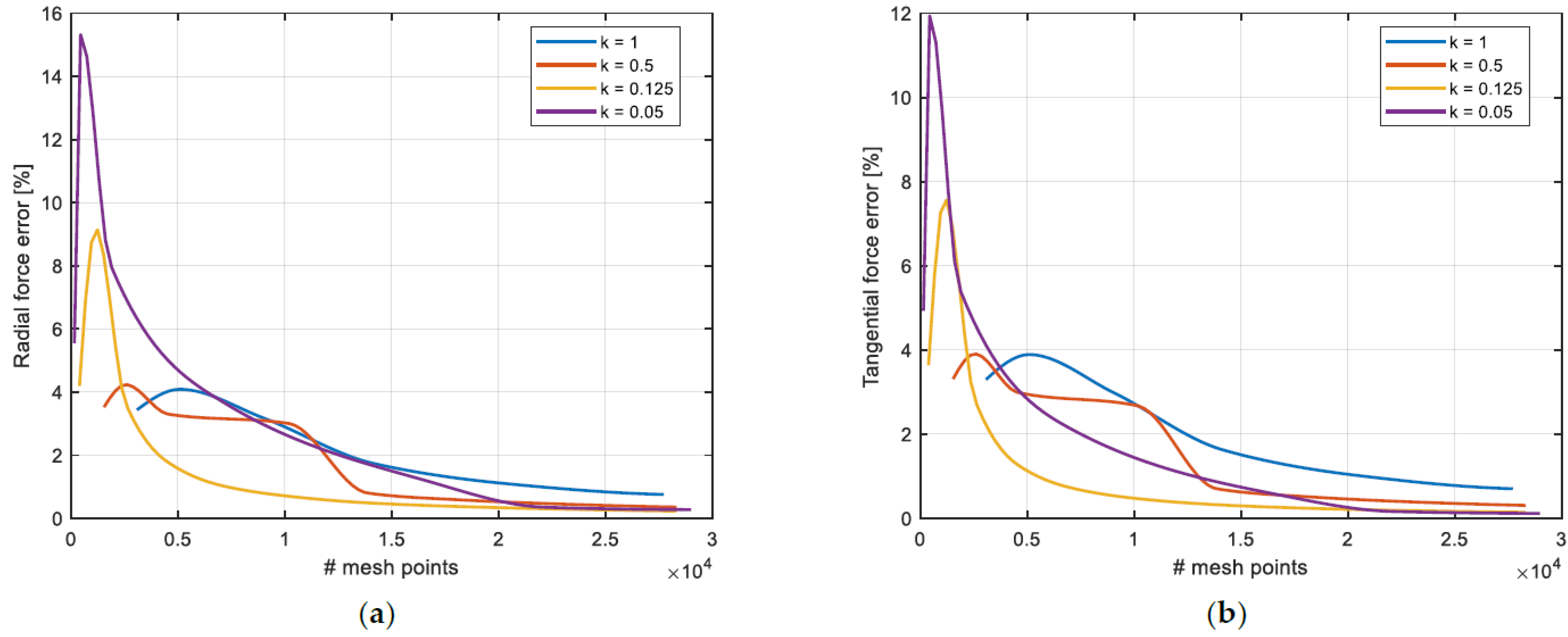
For every SFD configuration, the mesh independency check was performed considering a structured grid. Both rectangular and squared grids were considered, and the final number of elements adopted was selected with a trade-off between numerical accuracy and computational time. The evolution of the radial and tangential force relative error with the number of mesh points is reported.
For the sake of brevity, only the evaluation conducted for SFD F is reported. The number of axial points Nz is selected and the tangential point are evaluated as with . When , the elements are squared.
The evolution of the radial and tangential forces as a function of the number of mesh points and for some values of
(0.05, 0.125 0.5, 1) is shown in
Figure 10. Increasing the number of mesh points both errors reach an asymptote. When
is reduced, i.e., when for the same number of axial points, the number of tangential points is reduced, the shape of the error evolution is flat. Generally, a relative error below 1% can be considered acceptable. To keep the alculation time low, for SFD F, the mesh configuration selected has
and approximately 1 × 10
4 mesh points.
4. Application
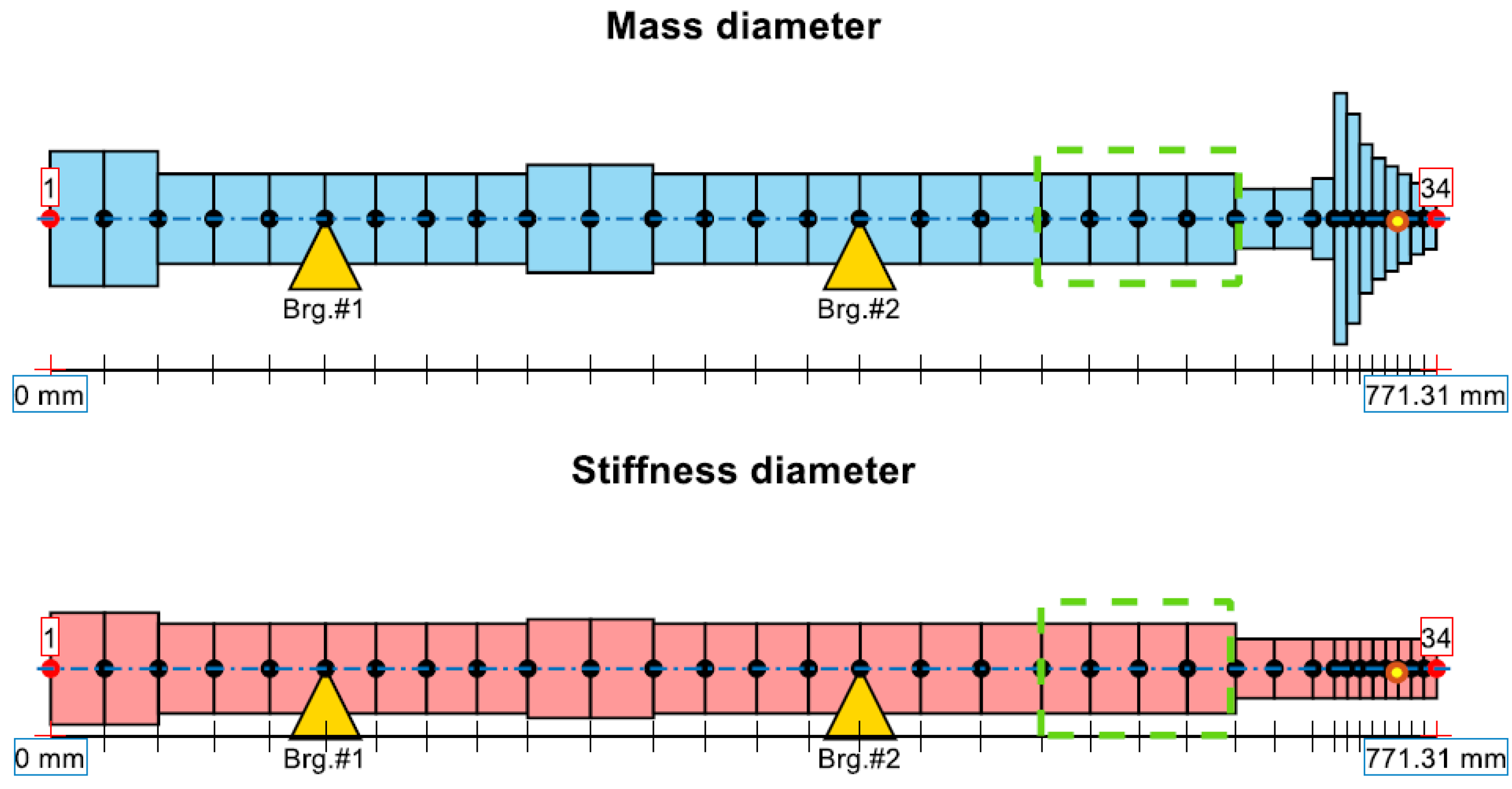
The proposed model has been integrated in the finite beam element analysis of a high-speed centrifugal compressor coupled with a gear element. The shaft of the machine is long
and the nominal diameter is
. The impeller is
long and has a maximum diameter of
while the minimum one is
. The finite element discretization of the structure, with a total of 34 nodes, is shown in
Figure 11.
As shown in
Figure 11, the stiffness and mass diameter are different for the different elements. The yellow triangles represent the two roller element bearings. The green rectangle represents the region where a sealing element is placed. The scheme of the machine represents an actual application while the application investigated in the next pages is a hypothesis. In the analysis an unbalance force of
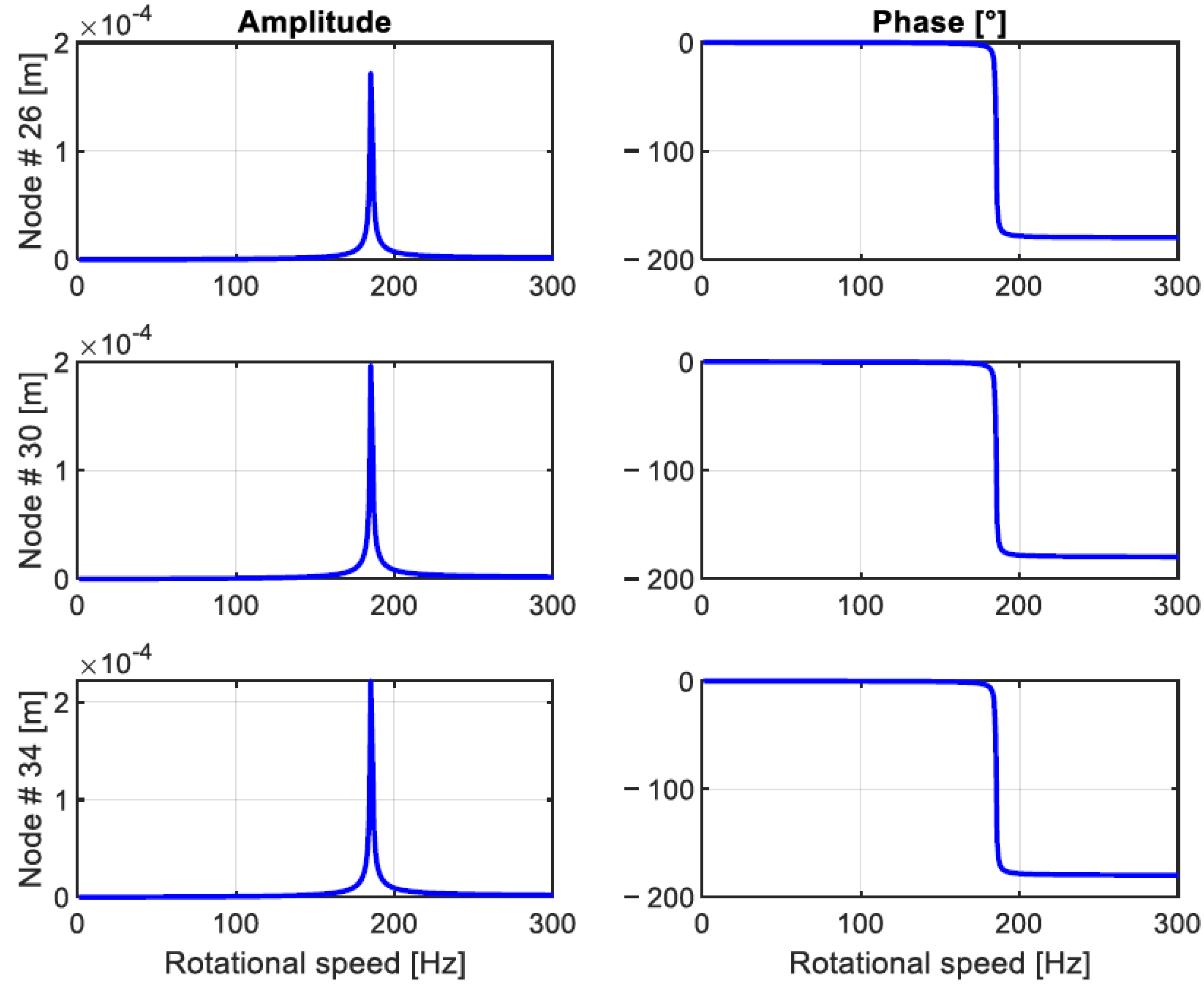
is placed in the yellow node of the impeller (node 31). The effect of the seal is not taken into consideration while the attention is focused on the reduction of the vibration of the machine, focusing on the impeller. The operational speed range of the compressor goes from
and
is considered as the operating frequency. The forced responses to the unbalance at three nodes of the impeller are shown in
Figure 12. It is possible to see that, due to the characteristics of the bearings, the system is barely damped and when crossing the natural frequency, at
, the vibration’s amplitude is, in the last node, higher than
. Due to the small gaps between the impeller and the cage and to reduce the aerodynamic losses, it is important to reduce as much as possible the level of the vibration.
To reduce the vibration peak, a SFD is applied in parallel with the first bearing. The new structure is shown in
Figure 13. The SFD is supposed to be supported by an external squirrel cage defined by its own mass (m
cage) and stiffness (k
cage), respectively. Moreover, the squirrel cage acts as a centering mechanism. The SFD introduces an external source of damping (c
SFD) and added mass (m
SFD).
For simplicity, a plain SFD without grooves, feeding system, and seals is considered. The geometrical characteristics of the SFD and the properties of the ISO VG 46 oil considered are listed in
Table 2.
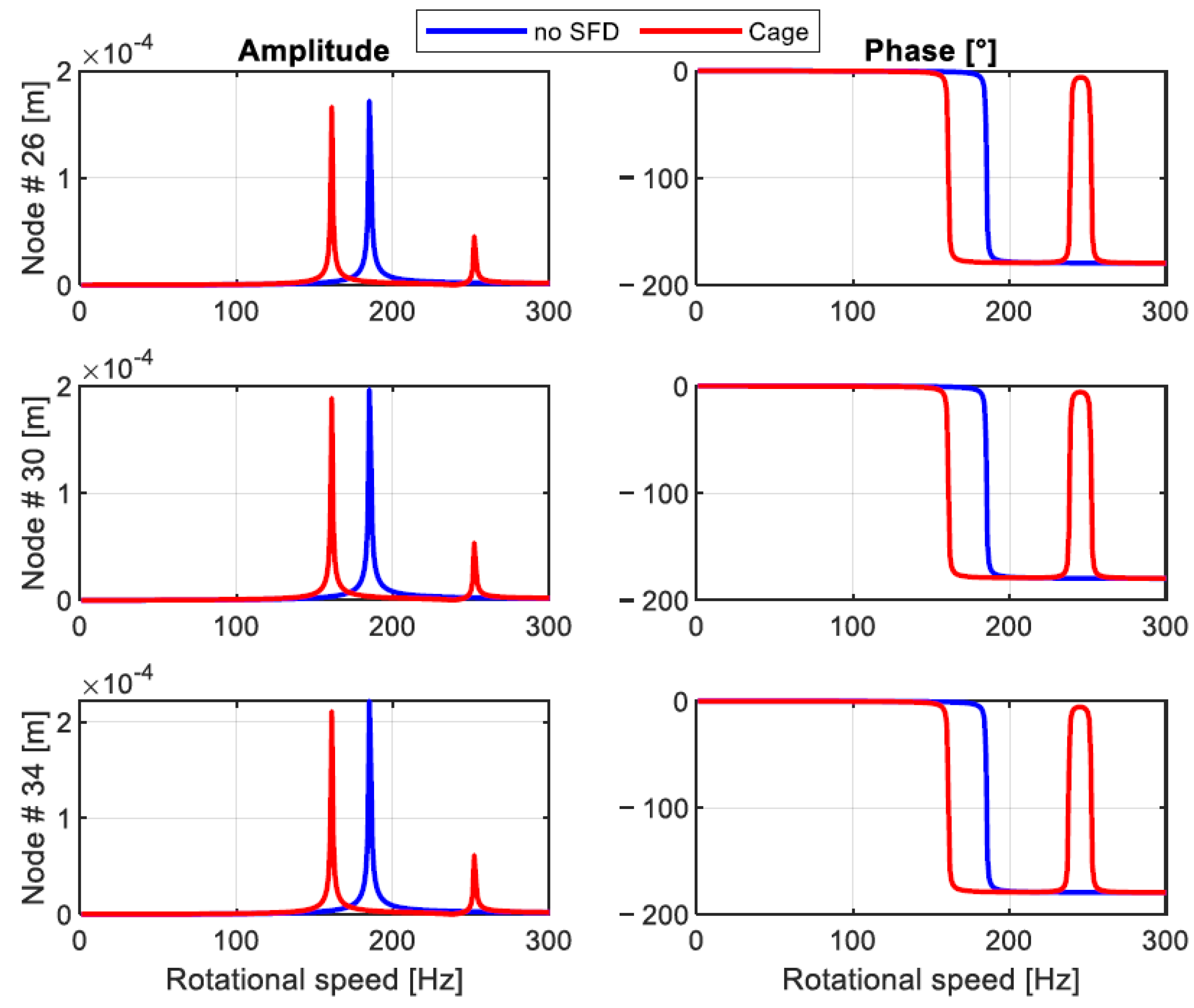
At first, the forced response of the configuration with the squirrel cage but without considering the presence of the oil is performed. The comparison between the two forced responses for the same impeller nodes considered in
Figure 12 is shown in
Figure 14.
As it is possible to see from
Figure 14, the introduction of the squirrel cage significantly changes the forced response. The introduction of the squirrel cage has the effect of a tuned mass damper. The resonance peak at
is moved to
. Moreover, a second resonance peak is present at
.
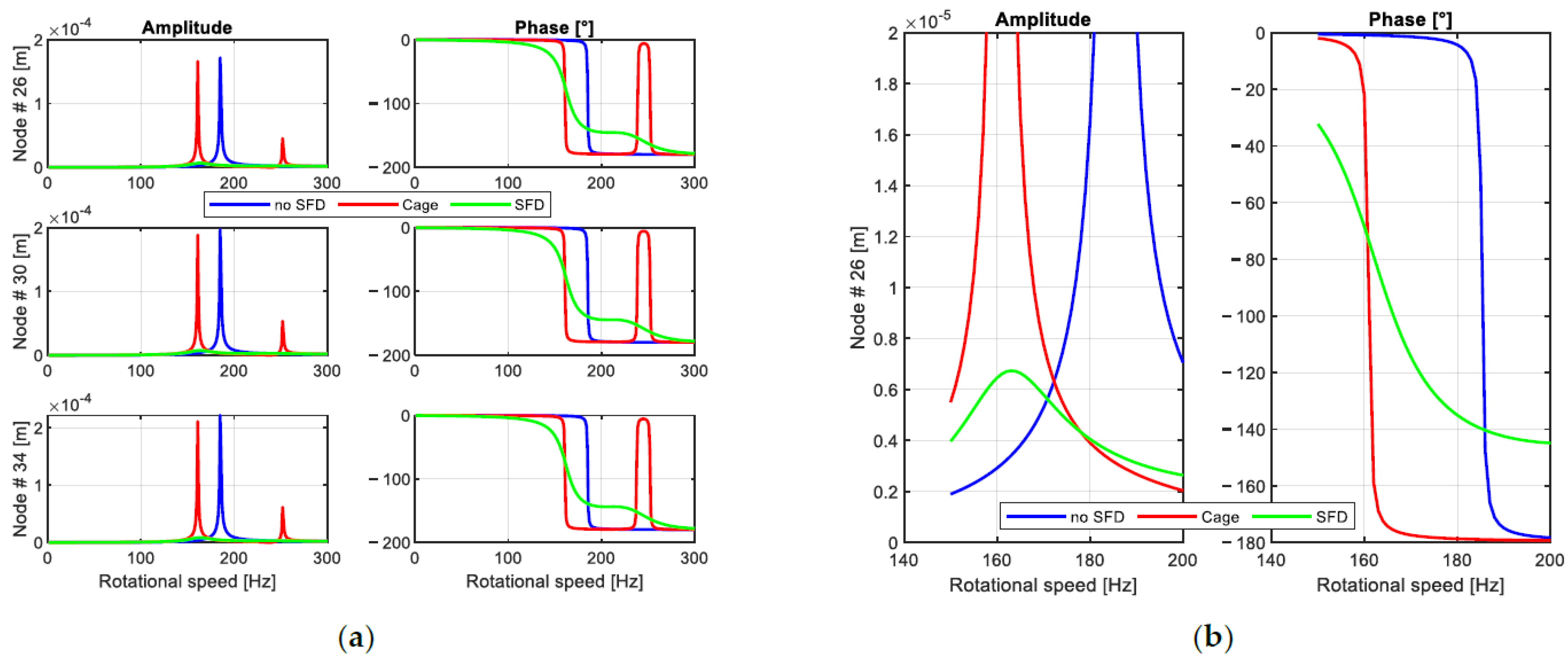
Then, the previously mentioned SFD is considered for the forced response. The comparison between the forced response between the original configuration, the configuration with the squirrel cage, and the SFD configuration is shown in
Figure 15. The introduction of the SFD is strongly effective in the reduction of the level of the vibration peak.
Then, the effect of some geometrical parameters on the forced response of the system is evaluated. As previously mentioned, the operating frequency considered is
. Therefore, considering the evolution of the forced responses shown in
Figure 15, the frequency range from
to
is considered for the following analysis.
4.1. SFD Clearance
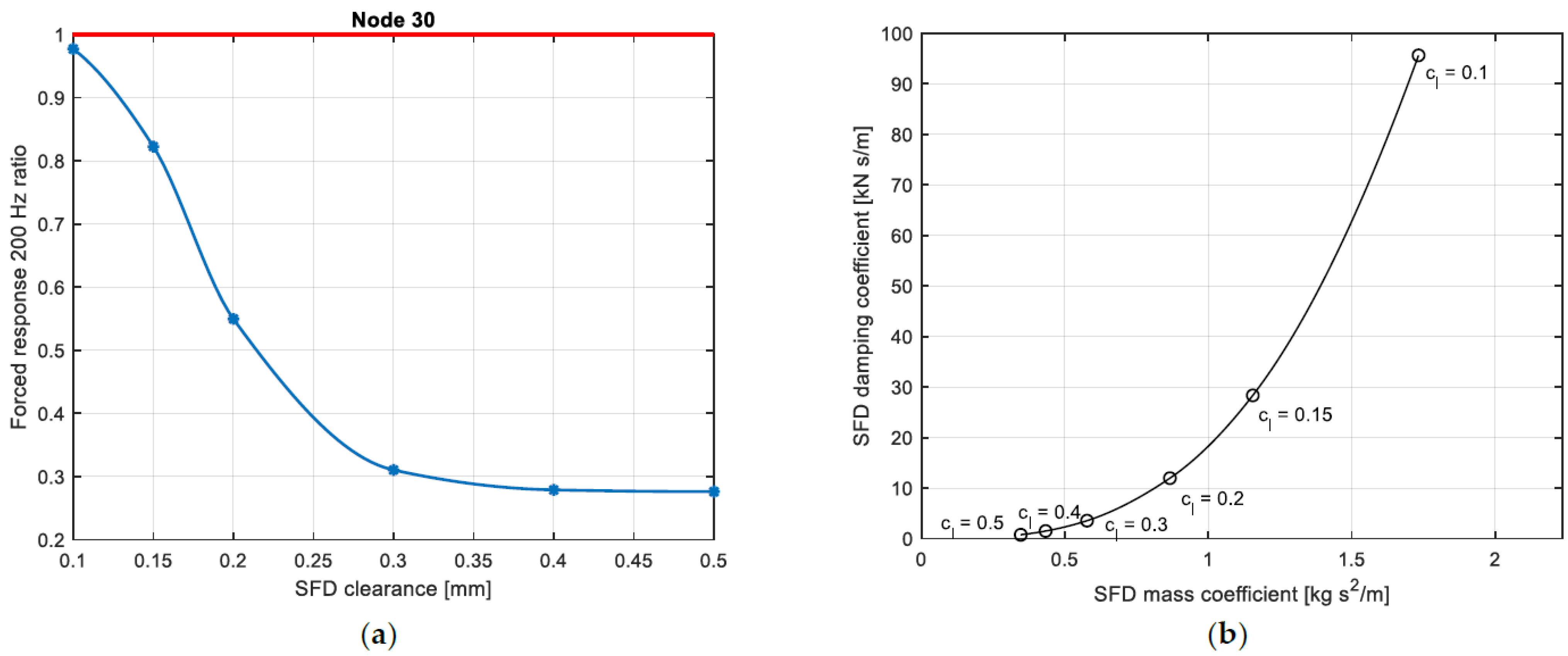
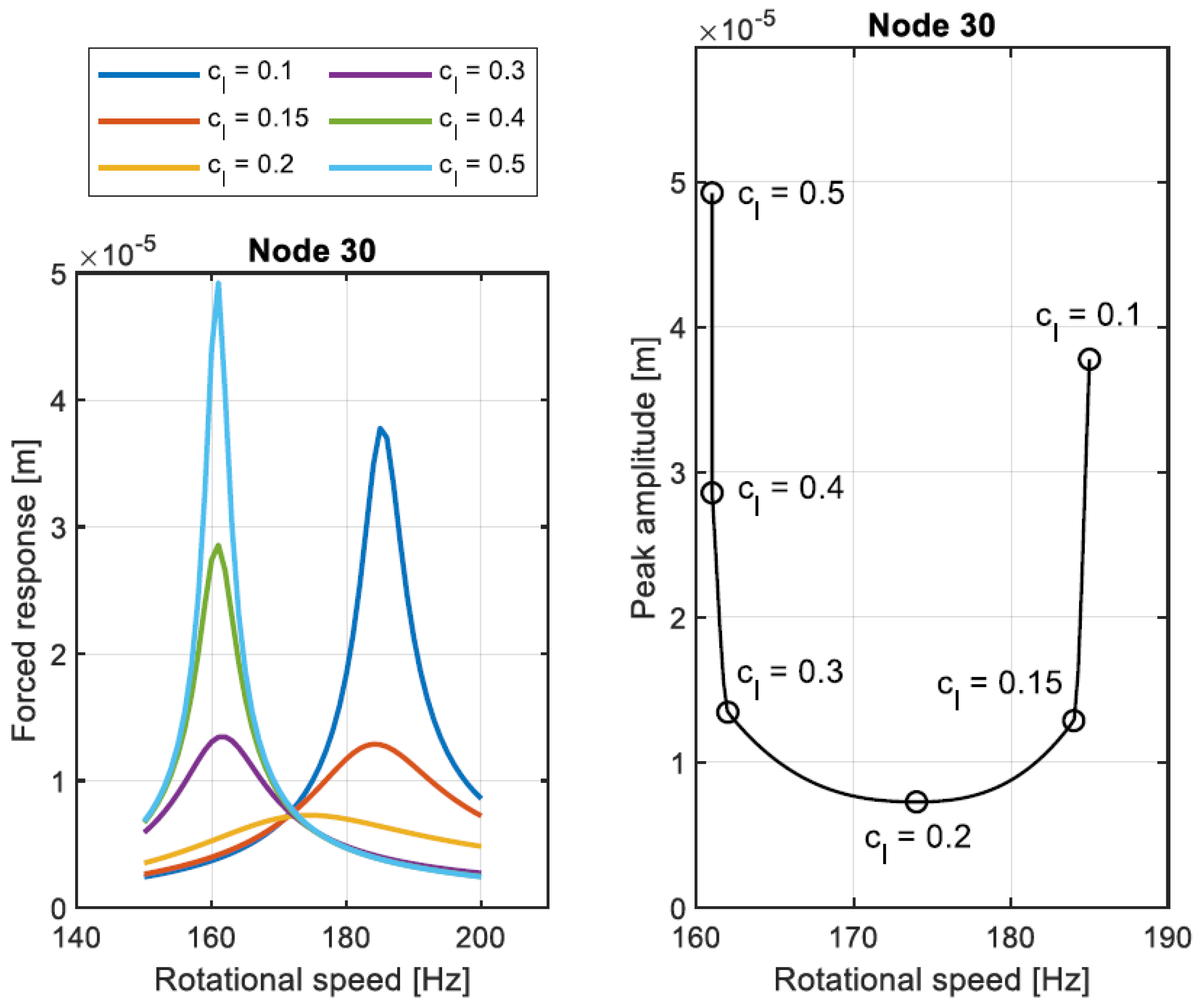
The first parameter to be investigated is the clearance of the SFD. The ratio between the forced response at
of the configuration with the SFD and the original one is shown in
Figure 16. The forced response decreases with the increase of the SFD clearance even though the damping coefficients increases when the SFD clearance is decreased. This behavior is related to the increase of the resonance frequency when the SFD clearance is reduced. Therefore, a higher level of vibration is obtained at
(see
Figure 17).
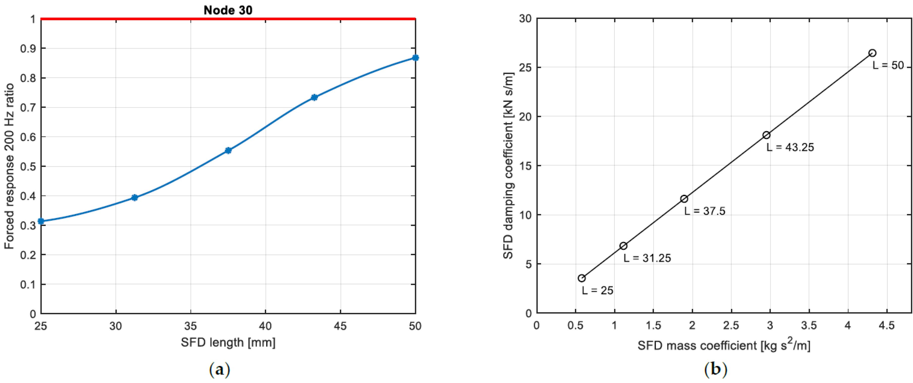
4.2. SFD Length
The effect of the length of the SFD on the forced response is investigated. For this analysis, the selected SFD clearance is
because it minimizes the vibration level at
and guarantees an acceptable level for the resonance peak vibration. The ratio of the forced response at
for the original configuration and the configuration with the SFD is shown in
Figure 18a. The minimum forced response is obtained when the shortest SFD is considered. The force coefficients of the SFD increase with the SFD length, see
Figure 18b. Therefore, also in this case, the most suitable SFD to reduce the vibration level at
is the one characterized by the lowest force coefficients.
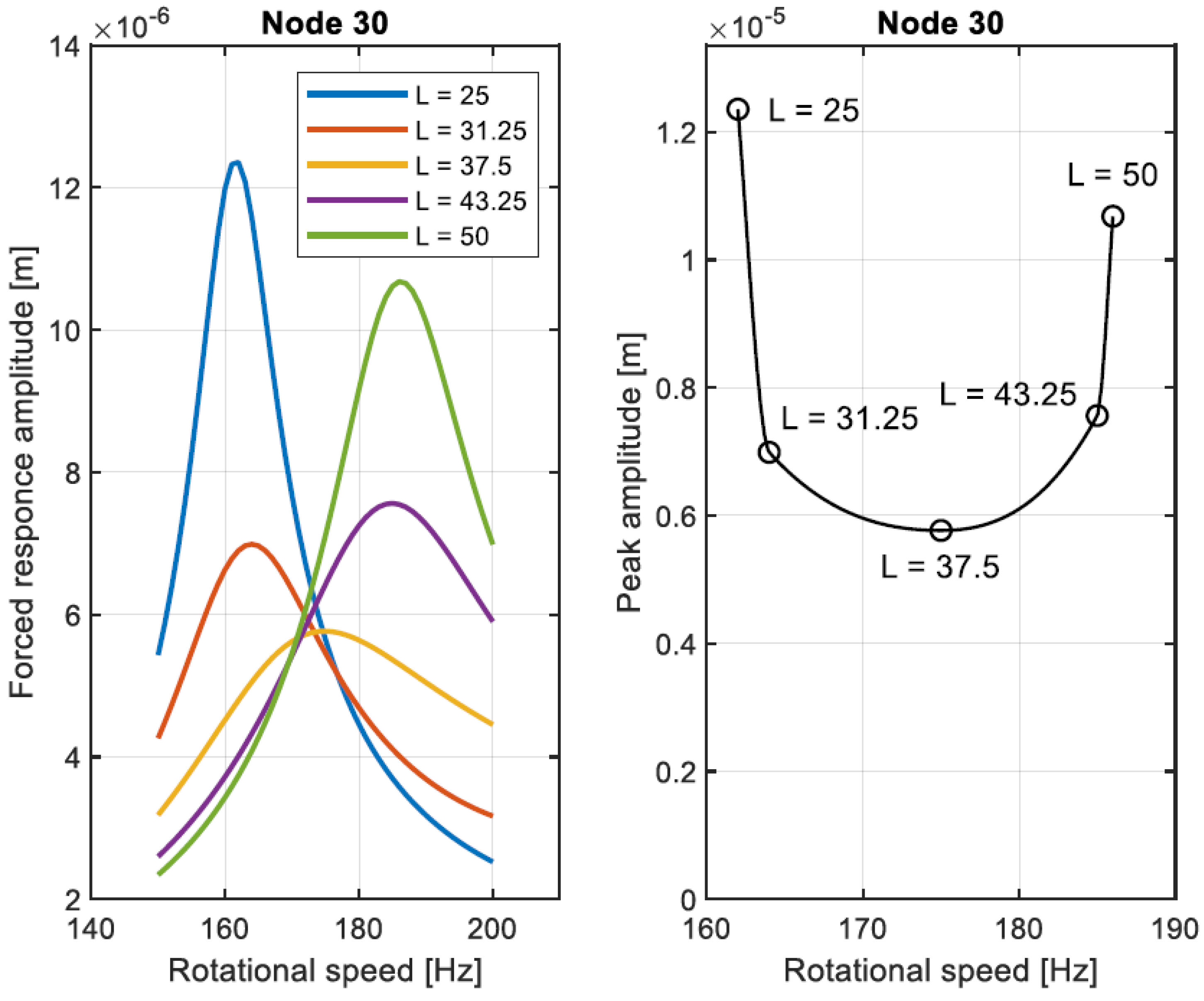
The comparison between the forced responses obtained considering the different values of length of SFD is shown in
Figure 19. Moreover, in this case, the results are reported in the frequency range of interest. It is possible to see that the minimum forced response at
is obtained with the shortest damper. On the contrary, the minimum of the vibration peak is obtained when
as shown in the right part of
Figure 19. Therefore, the proper SFD configuration must be selected according to the optimization required.
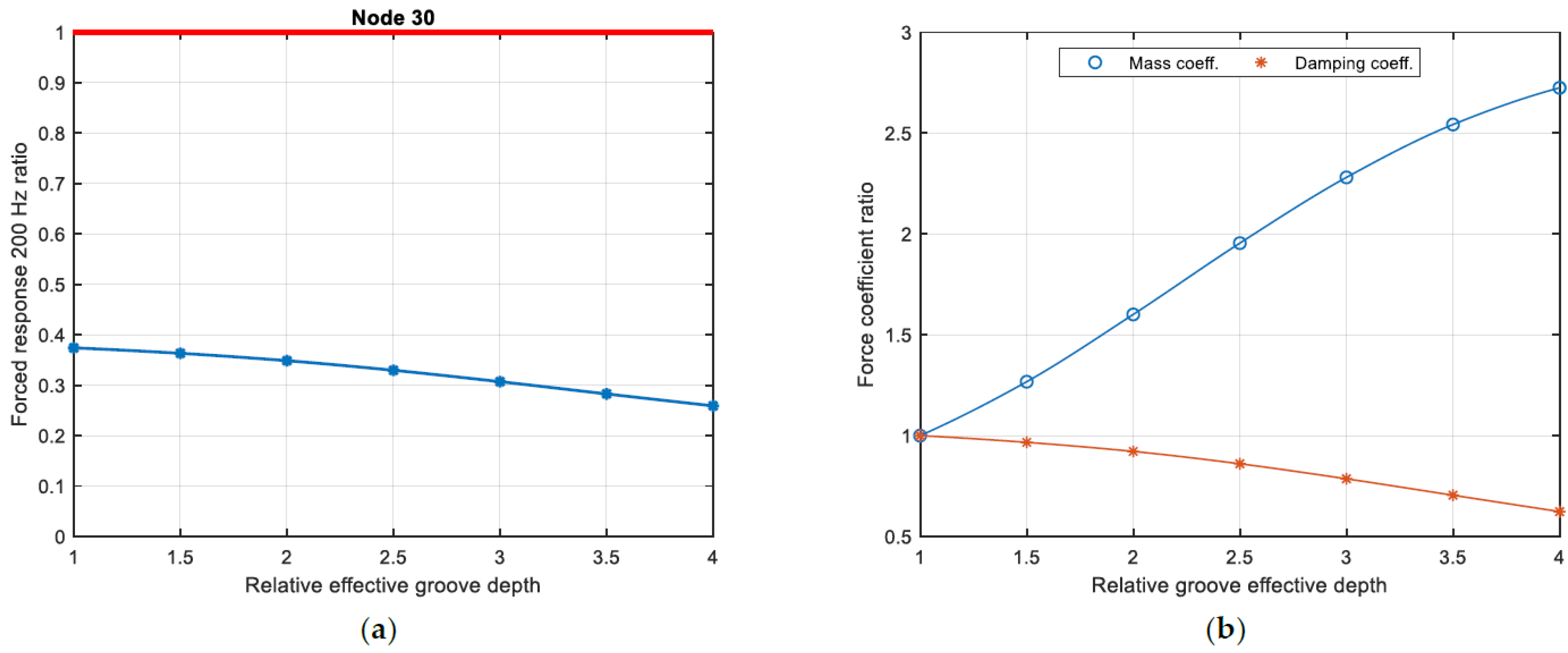
4.3. Groove Effective Depth
Another tuning parameter that can be selected for the geometry of the SFD is the effective depth of the groove. For this reason, different values of
have been investigated. For convenience, the relative value of the effective groove depth is considered (
). The ratio of the forced response at
for the original configuration and the configuration with the grooved SFDs is shown in
Figure 20a. The clearance considered is
and the lands of the SFD have a length of
. The groove length considered is
and it is placed in the center of the SFD. When the effective groove depth is one, the damper geometry results in a grooveless damper of length
. From the analysis shown in
Figure 20a, the higher the groove depth, the lower the forced response at
. The evolution of the ratio between the SFD force coefficients for the different values of the relative effective groove depth and the values obtained when
is shown in
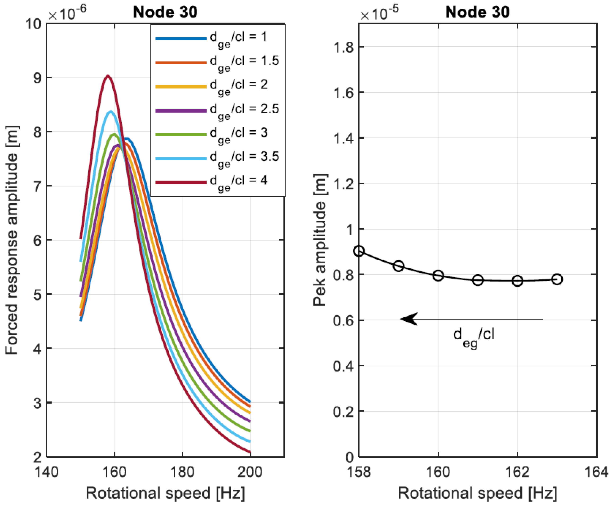
Figure 20b. Increasing the groove depth, the damping coefficient is reduced while the mass coefficient is highly increased. The evolution of the forced responses for the considered frequency range is shown in
Figure 21. Moreover, in this case, the configuration that minimizes the forced response at
is not the one that minimizes the amplitude of the peak.
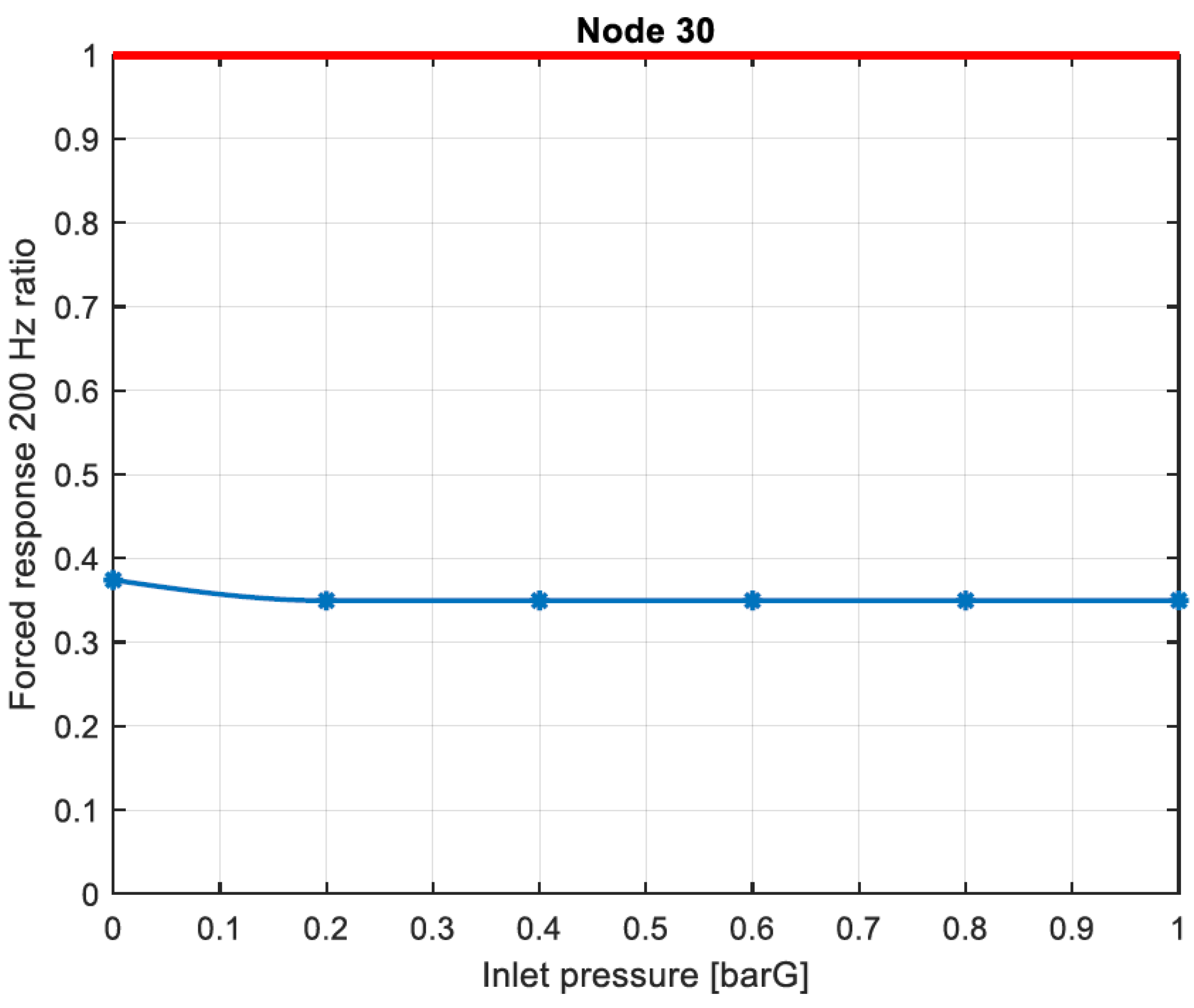
4.4. Feeding Pressure
In this section, the feeding system is considered. The SFD considered has a length of
and clearance equal to
and the diameter of the holes is considered equal to
. Moreover, the coefficient
is considered as
. The effect of the feeding pressure on the forced response has been investigated. The ratio of the forced response at
for the original configuration and the configuration with SFDs is shown in
Figure 22. When the feeding pressure is considered zero, the feeding system is not included in the modeling. The presence of the feeding system seems to have a small impact on the forced response at
and the inlet pressure is not influencing the forced response.
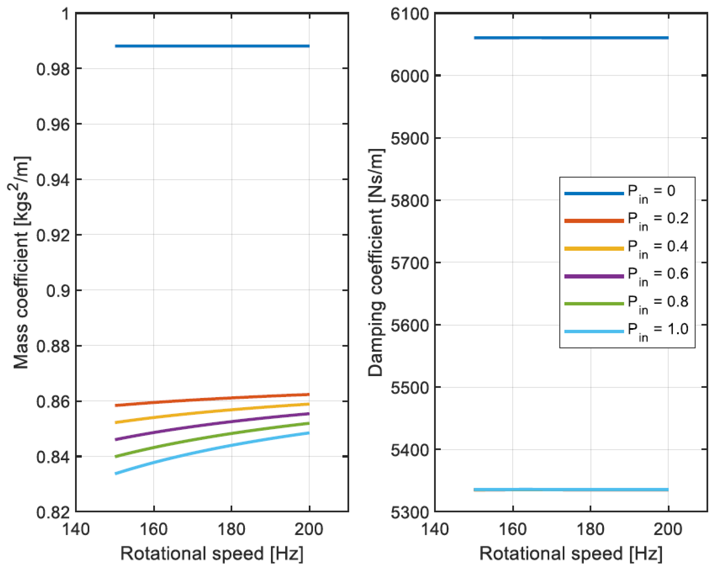
If the feeding system is not considered in the modeling and no cavitation or air ingestion is present, both the direct SFD force coefficients are equal and constant with the tested frequencies. On the contrary, when the feeding system is modeled, the xx and yy force coefficients are slightly different. Moreover, the mass coefficients show a dependency with the frequency which is more evident when the feeding pressure is increased, as shown in
Figure 23.
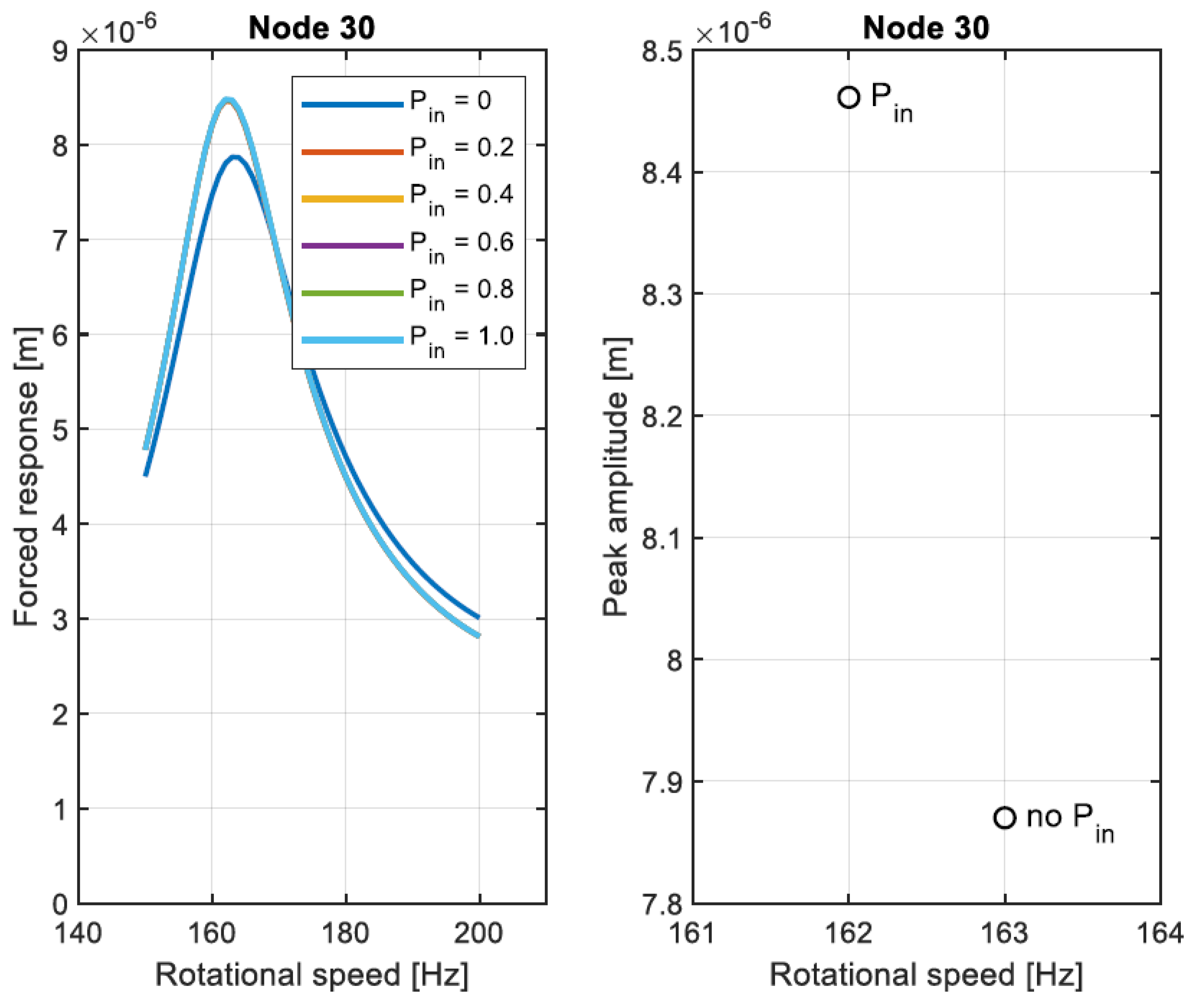
The differences in the force coefficients shown in
Figure 23 determine different forced response between the modeling with and without the feeding system (
Figure 24). On the contrary, the evolution of the mass coefficient with the rotational speed does not have an impact on the forced response.
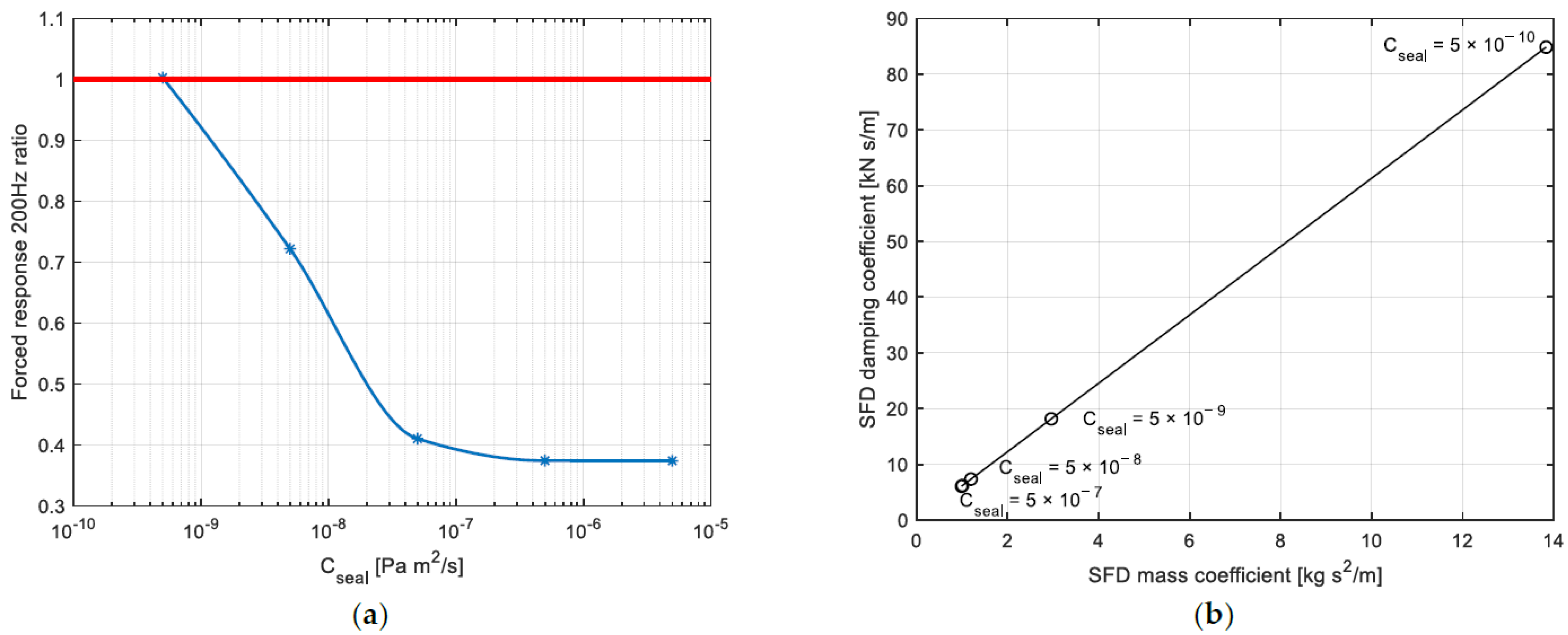
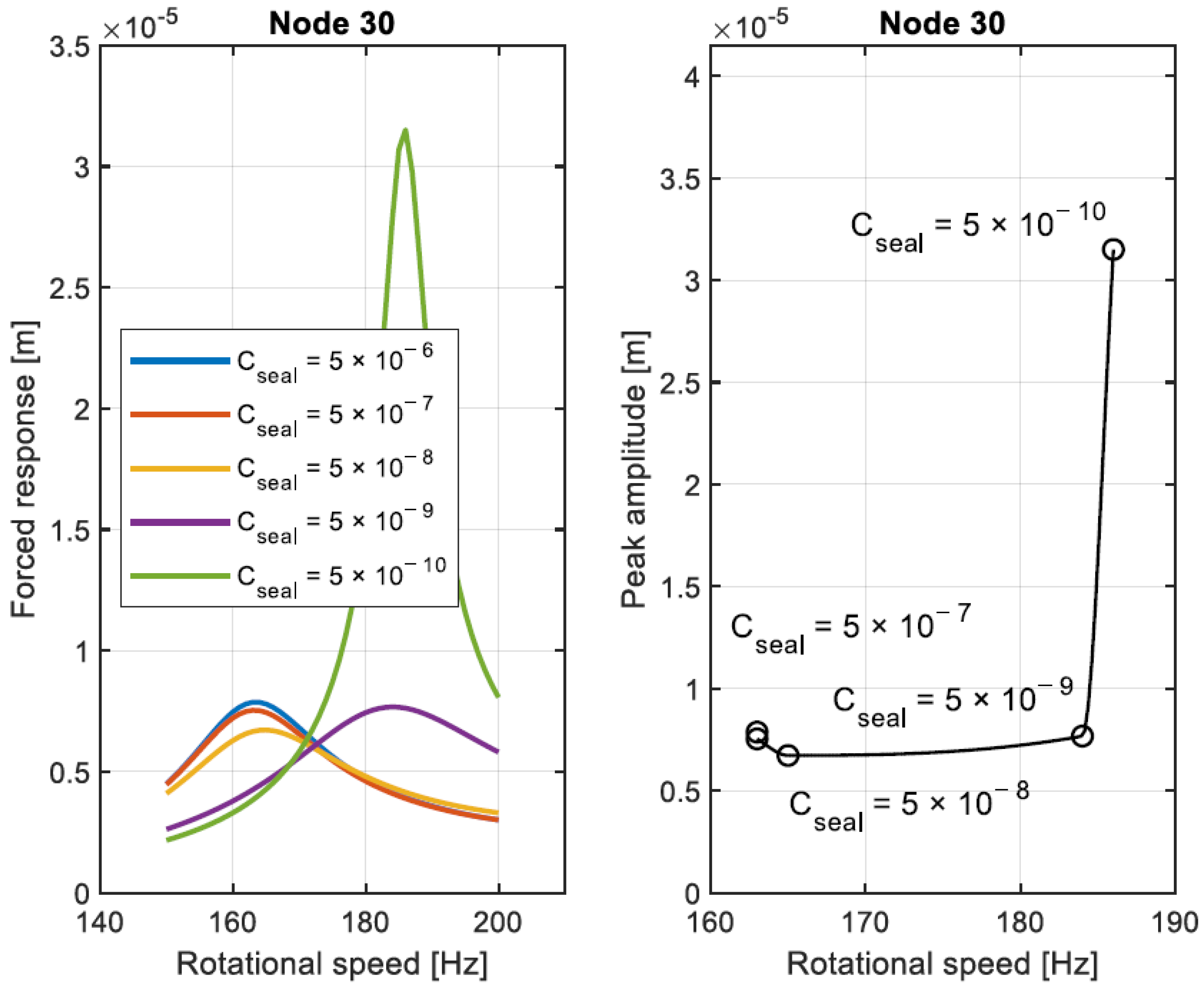
4.5. End Seals
For convenience, the effect of the sealing mechanism is shown considering the overall seal coefficient
. The highest value of
corresponds to the open ends condition while the lowest value of
corresponds to the ideal condition of complete sealing. The ratio of the forced response at
for the original configuration and the configuration with the sealed SFDs is shown in
Figure 25a. Increasing the sealing effect determines an increase of the forced response at
at node 30. The evolution of the force coefficients with
at
is shown in
Figure 25b. Increasing the sealing effect determines an increase of both the force coefficients of the SFD.
The evolution of the forced responses for the considered frequency range is shown in
Figure 26. Moreover, in this case, when the force coefficients are increased, the frequency of the peak of the forced response increases.
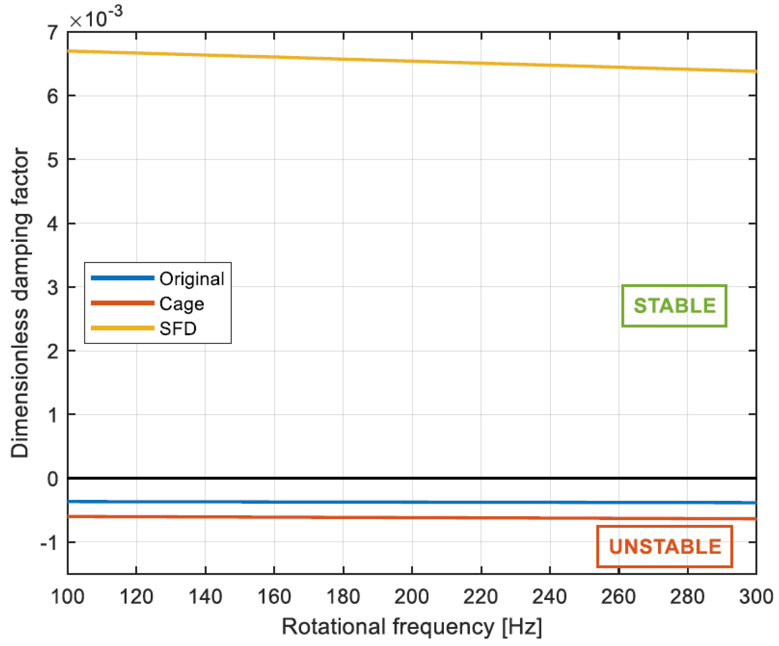
4.6. Correction of an Instability
In this section the effect of the seal placed before the impeller is considered as source of instability. The stiffness matrix at the nodes of the seal is introduced as follows:
The parameter determines whether the compressor is affected by instability. The effect of on the stability of the system is investigated. The first instability is present at . However, the system is unstable for the whole frequency range only when . For this reason, our analysis is focused at .
The same architecture shown in
Figure 13 is considered. The damping introduced in the system by the SFD tends to have a stabilizing effect. The dimensionless damping factor is studied as an indication of the stabilizing effect. This indicator is defined as:
The SFD considered is similar to that described in
Table 2 but now the clearance is set to
. The dimensionless damping factor for the original system, system with the cage, and the system with the SFD is shown in
Figure 27. Both the original system and the system with the cage are affected by instability. On the contrary, when the SFD is added to the system the correction of the instability is achieved.


