Article

An Iterative Modified Adaptive Chirp Mode Decomposition Method and Its Application on Fault Diagnosis of Wind Turbine Bearings

1
Department of Mechanical Engineering, North China Electric Power University, Baoding 071003, China
2
Changchun Power Supply Company, State Grid Jilin Electric Power Company Co., Ltd., Changchun 130021, China
3
Harbin Boiler Company Limited, Harbin 150046, China
*
Author to whom correspondence should be addressed.
Machines 2022, 10(8), 704; https://doi.org/10.3390/machines10080704
Submission received: 13 July 2022 / Revised: 14 August 2022 / Accepted: 15 August 2022 / Published: 17 August 2022
(This article belongs to the Section Machines Testing and Maintenance)

Abstract

:
Wind turbine bearings usually work with strong background noise, making the faulty properties difficult to extract and detect. To accurately diagnose the faults of rolling bearings in wind turbines, an iterative modified adaptive chirp mode decomposition (IMACMD) method is proposed in this paper. Firstly, an envelope interpolation method is employed to preliminarily determine the iterative mode number and guide the potentially initial frequency selection. Secondly, the upper limits of the iterative mode number and the initial frequency are further determined through correlation analysis. During the iteration process, the optimal weight factor of the reconstructive input signal, which is the residual signal of the previous iterative decomposition, is determined according to the new designed ensemble L-Kurtosis index. Experimental and engineering signals are used to validate the proposed IMACMD method. Comparisons with the conventional methods demonstrate the superiority of this proposed method. It is shown that this method can not only identify the weak features for single faults but also separate the multiple features for compound faults.

1. Introduction

Rolling bearings are key supporting components and have been widely used in a lot of industrial applications, such as high-speed trains, helicopter drive trains, wind turbines, etc. The running state of bearings greatly affects the safety of the system [1], since their unexpected failure leads to machinery breakdown or even catastrophic accidents [2]. Due to the reasons of heavy load, long term, and harsh operation environment in modern industry, the critical bearings in rotating machines have high potential of being damaged. Therefore, it is of great significance to accurately diagnose the bearing faults [3]. The damage may be concentrated on either one part (single fault) or multiple parts (compound fault). Compared to a single fault, compound faults are more harmful to the bearings [4] since they have mutual-coupling and cross-influence effects on the neighboring components [5]. Usually the diagnosis method for a single fault is difficult to use for compound faults [6,7]. Therefore, new diagnosis methods that are not only effective for both single and compound faults, but also qualified to accurately identify the faulty types and locations, are urgently requested.
At present, the vibration-based analysis method is the most convenient and widely employed bearing fault diagnosis technology, though the incipient failures cause some changes to the operating condition information in the collected vibration signals. According to the dynamics and fault mechanism, when a local injury appears on the rolling bearing, the high-frequency structural resonance will also be reflected in the bearing system [8]. The fault characteristic is generally regarded as contained in a periodic impact signal [9]. In theory, when the periodic impacts match the theoretical properties of the bearing, the fault type and location can be determined. In practice, due to the influences of many factors such as the shaft vibration, gear meshing, electromagnetic interferences, and external environmental issues, there may be harmonics, accidental pulses, and noises in the vibration signal [10]. Consequently, a weak fault signal is difficult to identify [11]. More seriously, when the compound faults occur, the coupling effect between two different faults may make the fault shocks overlap and even compensate each other, making the fault shocks become weaker and the compound fault diagnosis much more challenging [12].
In the past few decades, incipient fault diagnosis on rolling bearings has attracted the extensive attention of many scholars, who have carried out a series of studies for guiding industrial applications [13,14,15]. The popular and powerful signal-processing algorithms in bearing fault diagnosis mainly include spectral kurtosis (SK), deconvolution algorithms, and decomposition methods. As evolved versions of SK, SKRgram [16], Infogram [17], Autogram [18], and Accugram [19] are still restricted by the best frequency band selection [20] and the fixed spectral segmentation strategy, which may lead to the loss of some key faulty information [21]. The deconvolution algorithm, such as the minimum entropy deconvolution (MED) [22], maximum correlated kurtosis deconvolution (MCKD) [23], multipoint optimal minimum entropy deconvolution adjusted (MOEDA) [24], and cyclostationary blind deconvolution (CYCBD) [25], iteratively updates the filter to make the target evaluation index of the output signal reach the optimal value, so that the fault-affected signal can be recovered [26]. The performance of deconvolution algorithm greatly depends on the selection of the objective function and the filter length, which limit the practical application of the deconvolution methods [27]. Both the deconvolution and SK methods mainly focus on the extraction of the dominant fault features, whereas the secondary fault feature may be ignored while processing the vibration signals of the compound faults [28]. The signal decomposition methods, such as empirical mode decomposition (EMD) [29], local mean decomposition (LMD) [30], singular spectrum decomposition (SSD) [31], and variational mode decomposition (VMD) [32], are designed to decompose the signals into mode components of different frequency bands and separate the fault characteristic signals from the interference signals. As a very suitable technique for bearing fault detection [33], the main disadvantages of signal decomposition methods are as follows: (1) The original vibration signal will be decomposed into many sub-components, making the processing results very complicated, and (2) many parameters need to be well preset, since the satisfactory analysis results depend on the accurate setting of each parameter [34].
As a novel non-stationary and nonlinear signal analysis algorithm, adaptive chirp mode decomposition (ACMD) is developed based on the greedy search algorithm [35] and is able to extract the particular mode containing rich characteristic information without other redundant modes. The mode obtained by ACMD is a band-limited signal in which the primary energy is concentrated around a center frequency [36]. Compared with the aforementioned analysis methods, ACMD requests fewer preset parameters. Different from EMD, LMD, SSD, and VMD algorithms, which separate all the modes simultaneously, ACMD only obtains a particular mode containing rich characteristic information at a time to improve the time-frequency resolution. ACMD has been applied to the fault diagnosis on rolling bearings by scholars [37,38]. The authors have also studied this method for rolling bearing fault diagnosis, and more details can be found in [39].
However, most of the previous work focuses on single faults, and few of them have paid attention to compound faults, which can also take place in rolling bearings. To promote existing methods such as ACMD being effective in feature extraction for both single and compound faults, the following three issues need to be primarily considered: (1) The instantaneous frequency initialized in ACMD should be determined adaptively without prior knowledge, (2) proper modifications need be carried out to improve current methods such as ACMD to make them effective in detecting the all potential components for the weak and compound failures from the original signals, and (3) as the key parameter of ACMD, given that the weight factor directly affects the bandwidth of the estimated mode in ACMD, such key parameters need to be set reasonably. To resolve the aforementioned three issues, in this paper we propose an iterative modified adaptive chirp mode decomposition (IMACMD) method, which can further expand its application field from single faults to compound faults. What’s more, this method is able to detect all the sensitive components from the original signal.
Our proposed method primarily includes three steps. Firstly, an envelope interpolation method is adopted to preliminarily determine the number of decomposition modes and to guide the instantaneous ACMD frequency of each mode. Then, the modal number and the instantaneous frequencies can be obtained by deleting the strongly correlated modes.
Secondly, considering the interaction of the compound fault components, the input signal decomposed by the next iteration is reconstructed after filtering the specific frequencies through ACMD. In each iteration, the input signal of the first iteration is the original signal, whereas the subsequent input signal is the remaining one after removing the filtering signal.
Finally, based on the advantages of the time-domain L-Kurtosis and the frequency-domain L-Kurtosis, the ensemble L-Kurtosis (ELK) is designed as a new index. Under the guidance of the modal number and the instantaneous frequencies in the aforementioned steps, the new index, which considers both the cyclostationary process and the impulsiveness, is used to select the optimal weight factor (α) for each IMACMD decomposition mode.
Through these improvements, the above-mentioned issues are attempted to be solved. The feasibility of the new IMACMD method are verified by simulating, experimental, and engineering signals. At the same time, this paper also tries to compare SSD and SK, and discusses the superiority of the proposed method. Using the IMACMD method, more ideal fault diagnosis results of rolling bearings are expected to be obtained.
The remainder of this paper Is organized as follows. Section 2 describes the basic principles of ACMD, analyzes the effects of its key parameters, and proposes and discusses the signal evaluation index ELK. In Section 3, the particular implementation steps of the proposed IMACMD method, including the localization strategies for the number of iterations, the instantaneous frequency, and the weight factor of ACMD, are presented in detail. Subsequently, the effectiveness and the superiority of IMACMD are validated by the experimental signals and engineering signals in Section 4 and Section 5, respectively. Finally, conclusions are summarized in Section 6.

2. Theoretical Description and Characteristics Study on ACMD

2.1. Basic Theory of ACMD

Extended from VMD, ACMD is a novel algorithm for non-stationary signal decomposition and has obvious advantages in the processing of multi-component strong frequency modulation signals and excellent time-frequency resolutions [40]. Since ACMD is sensitive to the impact responses, it has been treated as a good choice to process the vibration signals for the bearing fault diagnosis [41].
The main parts of ACMD consist of a recursive mode extraction framework, an adaptive bandwidth updating rule, and a frequency initialization scheme based on Hilbert transform. For a nonstationary signal x(t), ACMD solves the optimization problem as follows:
min a m ( t ) , b m ( t ) , f m ( t ) p m ( t ) 2 2 + q m ( t ) 2 2 + α x ( t ) x m ( t ) 2 2
with
x m ( t ) = p m ( t ) cos 2 π 0 t f ˜ m ( t ) d t + q m ( t ) sin 2 π 0 t f ˜ m ( t ) d t
where pm(t) and qm(t) are both the de-chirped signals, α denotes the weight factor, fm(t) represents the instantaneous frequency, x ( t ) x m ( t ) 2 2 is the residue energy after the current estimated component is removed, and the square of the second derivative is employed to measure the bandwidth of the target mode.
The signal x(t) is discretized to a discrete signal whose time series is t = t 0 , , t N 1 , and the number of the sampling points is N; the discrete version of Equation (1) can be expressed as:
min u m , f m Θ u m 2 2 + α x G m u m 2 2
where Θ = Ω Ω , and Ω is a second-order difference matrix. u m = p m T , q m T T , p m = p m ( t 0 ) , , p m ( t N 1 ) T , q m = q m ( t 0 ) , , q m ( t N 1 ) T , and x m = x m ( t 0 ) , , x m ( t N 1 ) T . The kernel matrix G m is related to the demodulation frequency f ˜ m ( t ) and can be written as:
G m = C m , D m C m = d i a g cos ( φ ( t 0 ) ) , , cos ( φ ( t N 1 ) ) D m = d i a g sin ( φ ( t 0 ) ) , , sin ( φ ( t N 1 ) ) φ m ( t ) = 2 π 0 t f m ( t ) d t
x(t) is decomposed by minimizing the demodulation signal bandwidth, and the signal components are estimated one by one to achieve the accurate estimation on the multi-component chirp signals.

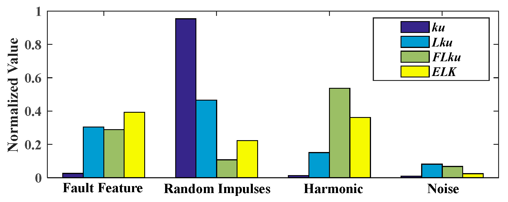
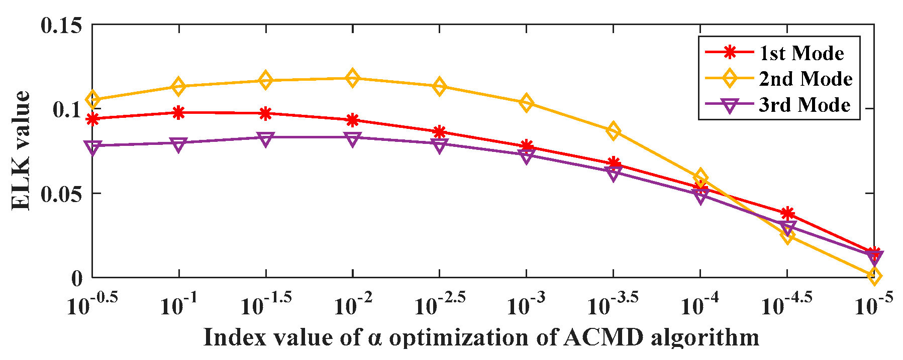
2.2. Ensemble L-Kurtosis Indicator

When rotating machineries are damaged, periodic pulse signals will appear. Such pulse signals are the most important basis for fault detection. In a weak noise environment, the time-domain features, including the pulses and periodicities, are easy to recognize. However, when the fault signal is fulfilled by noises, the fault characteristics are easy to bury in the time-domain waves but can be found in the spectrum. Although the bearing fault information exists in the full spectrum, most of the energy is concentrated near the natural frequencies. Ideally, a composite signal can be decomposed into a series of independent components, several of which contain the fault information and can be visually displayed in the envelope spectrum.
Appropriate signal characteristic evaluation criteria are of great significance for mechanical fault diagnosis. Kurtosis (ku) [42] is considered one of the sparsity measurements, since it can detect the impulsiveness of the signal. Similar to the traditional ku indicator, L-Kurtosis is defined as an alternative indicator to evaluate the variable distribution characteristics by extending the traditional moment principle [43], and it has better anti-interference and robustness properties than Kurtosis [44].
Assume that X = [ X 1 , X 2 , , X n ] is an independent sample from the cumulative distribution P(x), and X 1 : n X 2 : n X n : n is a random variable drawn from X. The rth L-moment μ r of the independent sample X is described as:
μ r = 1 r k = 0 r 1 ( 1 ) k r 1 k E ( X r k : r ) , r = 1 , 2 ,
where the expectation E ( X r k : r ) is expressed as:
E ( X j : r ) = r ! ( j 1 ) ! ( r j ) ! 0 1 x [ P ( x ) ] j 1 [ 1 P ( x ) ] r j d P ( x )
The 2nd and the 4th L-moments can be calculated as:
μ 2 = 0 1 x ( 2 P ( x ) 1 ) d P ( x )
μ 4 = 0 1 x ( 20 P 3 ( x ) 30 P 2 ( x ) + 12 P ( x ) 1 ) d P ( x )
Then the definition of L-kurtosis is expressed as:
L - Kurtosis = μ 4 / μ 2
However, L-Kurtosis pays more attention to the strength of the impacts rather than the regularity of the impacts. The spectrum of L-Kurtosis, which can be used to evaluate the cyclostationary process, is used in the fault diagnosis. Therefore, a new index is constructed by the virtue of L-Kurtosis and the spectrum of the L-Kurtosis. It is defined as
E L K = L k u · F L k u
where ELK represents the ensemble L-Kurtosis, Lku is the time L-Kurtosis, and FLku is the spectrum of the L-Kurtosis.
To investigate the performance of the above indexes, a simulating signal was constructed based on the vibration model in Section 2.3. As shown in Figure 1, the simulating signal consists of four components. Besides the fault feature and noise, random impulses from the electromagnetic interference frequency and the harmonic components of the shaft rotating appeared in the simulated signal. The detailed parameters are presented in Table 1. The normalized results of the four indexes used to calculate each simulated component are shown in Figure 2. The comparison shows that ku and Lku were most sensitive to the random impulses, rather than the fault impulses and harmonic components. On the contrary, Flku was most sensitive to the harmonic components. Obviously, ELK focused more on the cyclic impact characteristics than ku, Lku, and FLku. In addition, compared with Lku and FLku, ELK can employed better noise reduction. Considered a satisfactory indicator, ELK could accurately quantify the abundance of the periodic shocks. Consequently, it was able to capture the fault information and the harmonic information to the maximum extent.

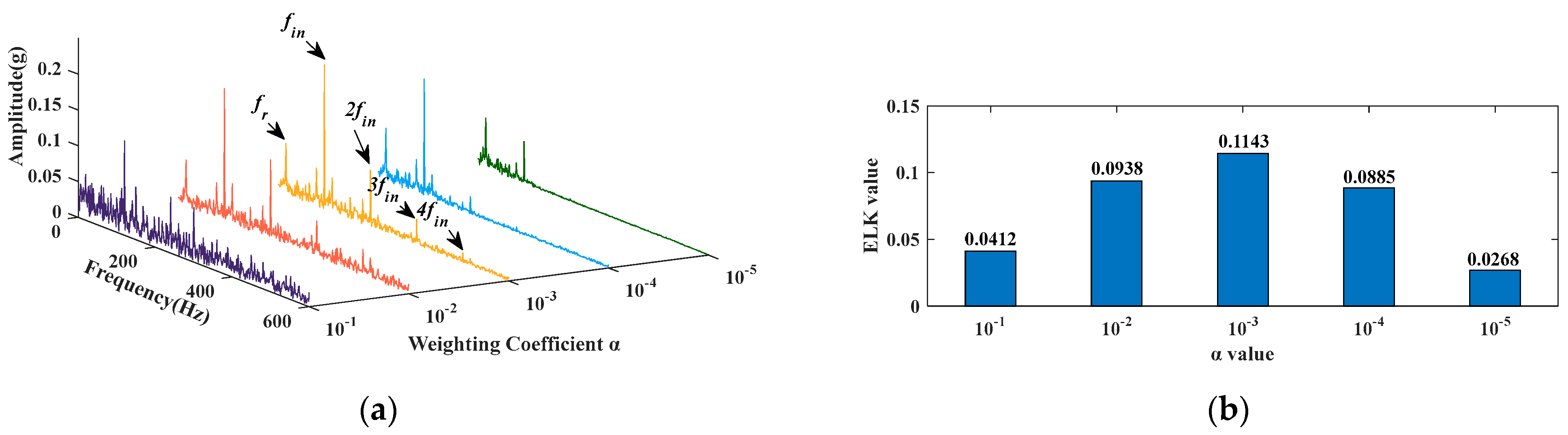
2.3. Research on the Influence of ACMD Parameters

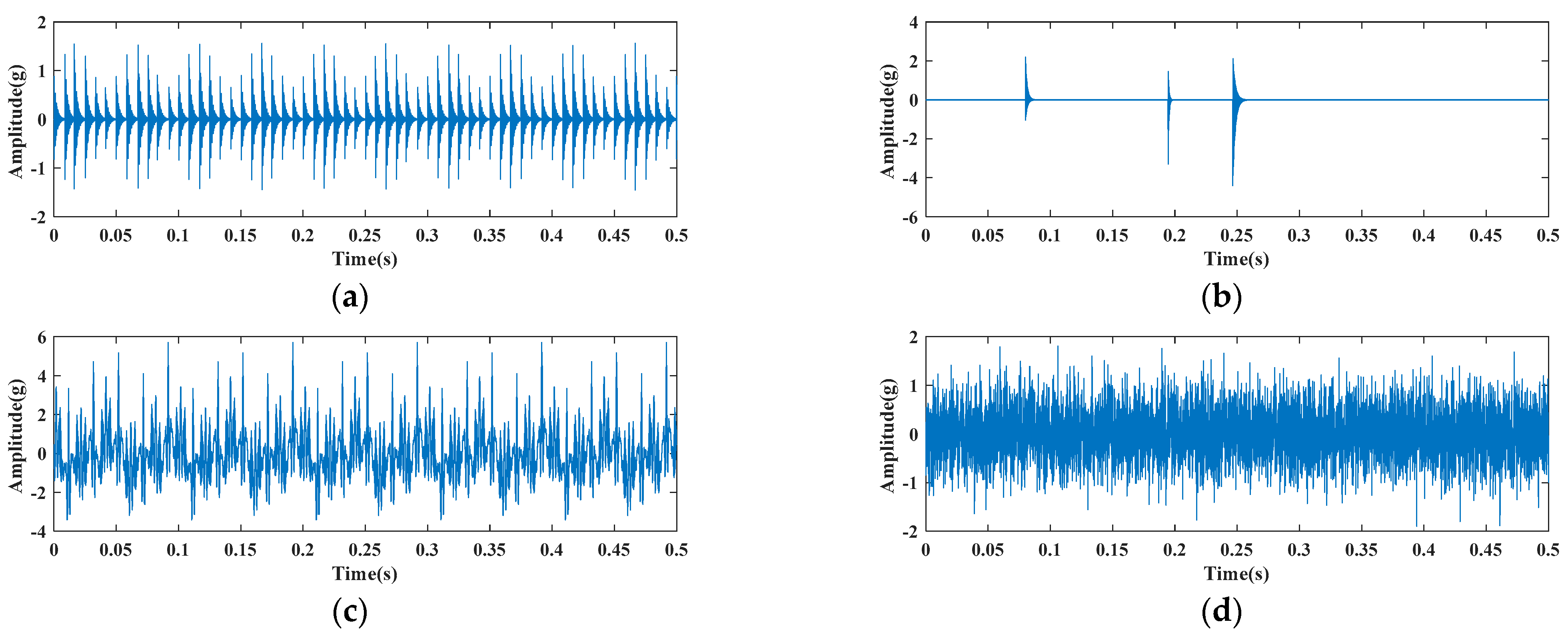
2.3.1. Bearing Fault Simulating Signal

As two significant parameters of ACMD, the optimization of the instantaneous frequency fc and the weight factor α has been studied by many scholars. However, which of these two parameters is more important has been rarely discussed in the previous works. To qualitatively study this topic, the observation signal of a single bearing fault is constructed as
x ( t ) = i = 1 I A i sin 2 π f n t s i ( t i T a γ i ) f a u l t   f e a t u r e + j = 1 J B j s j ( t j T j ) r a n d o m   i m p a c t s + k = 1 K C k sin 2 π f k t + ϕ k h a r m o n i c   c o m p o n e n t s + n ( t ) n o i s e
The simulated fault signal consists of the fault feature signal, the random impulses, the harmonic components, and the noise. In this simulating verification, sm(t) represents the impulse response function of the rotating machinery system and can be expressed as follows:
s m t = exp β m t cos 2 π f m t + ϕ m
where βm, fm, and φm denote the coefficient of the resonance damping, the resonance frequency, and the phase, respectively.
The parameter setting of the simulated signal is shown in Table 1. The sampling frequency fs = 12 kHz and the sample length Ns = 8192. The number of random impacts caused by the occasional shocks and the electromagnetic interferences on the machine was set as 3. The Gaussian distributed white noise n(t) = 0.5randn (1, Ns) was added to the simulating signal. In the meantime, an inner race weak defect signal was generated, with a fault characteristic frequency fin = 120 Hz. The components of the simulating signal are illustrated in Figure 1a,d. The resonant frequency band of the simulated inner race fault was set as 5500 Hz. On account of some uncertain interference components with high energy, the energy of this resonant frequency band was very weak. From the waveform illustrated in Figure 3a, the time intervals between two adjacent shocks did not match the period of the cycle impacts. Figure 3b shows the spectrum of the composite simulating signal; it can be seen that the main energy was not concentrated at 5500 HZ. Furthermore, the most important fault information at 120 Hz was invisible in the envelope spectrum depicted in Figure 3c.

2.3.2. Study on Decomposition Characteristics of ACMD with Different Parameters

Based on the variable-control method, the simulated signal x(t) was used to study the feature extraction effect of ACMD with different fc and α.
Firstly, the influence of fc on the ACMD filtering effect was analyzed. α was fixed to 0.1, whereas fc was set to 500 Hz, 1500 Hz, 2500 Hz, 3500 Hz, 4500 Hz, and 5500 Hz. The envelope spectra of ACMD filtering signals with different fc values are shown in Figure 4. When fc was set to the resonant frequency (fn = 5500 Hz) of the fault signal, the fundamental frequency (fin = 120 Hz) and the double frequency (2fin = 240 Hz) of the characteristic component could be effectively extracted. In the other five groups of ACMD filtering signals, the harmonic and the random impact information could be recognized, but there was little identifiable fault feature information. This indicates that more useful characteristics can be captured if fc is properly configured.
Subsequently, the effect of α on the ACMD algorithm was studied under the optimal instantaneous frequency condition, with fc = 5500 Hz. The envelope spectrum of each filtering signal of ACMD is shown in Figure 5a, with α set to 10−1, 10−2, 10−3, 10−4, and 10−5, respectively. According to the five envelope spectra, the following conclusions can be drawn: (1) The third spectrum (α = 10−3) had the highest fundamental frequency amplitude (fault characteristic), whereas the first and the fifth ones had the lowest amplitudes. (2) The interference components were obviously eliminated with the decrease in α, but the fault information was first enhanced and then attenuated. (3) When α = 10−3, the fault information extraction was obviously the most powerful, and fin~4fin were clearly visible. (4) After fc was set correctly, the further reasonable selection of α made the characteristic information much more clear. Figure 5b displays the histogram of the ELK indicators corresponding to different α values, which further validates the effectiveness of this indicator in evaluating the richness of the periodic impact components. Thus, ELK can be applied as the guidance indicator to optimize the parameter α for ACMD.
By the comparative analysis results in Figure 4 and Figure 5, it can be concluded that the weight factor had less impact than the instantaneous frequency on the execution effect of the ACMD algorithm. Therefore, the instantaneous frequency parameter should be accurately confirmed first, or else the fault characteristic information cannot be correctly captured. In order to effectively separate the optimal target mode from others, an innovative iterative ACMD fault diagnosis method based on the envelope interpolation and the correlation analysis is proposed; more details are presented in the subsequent sections.

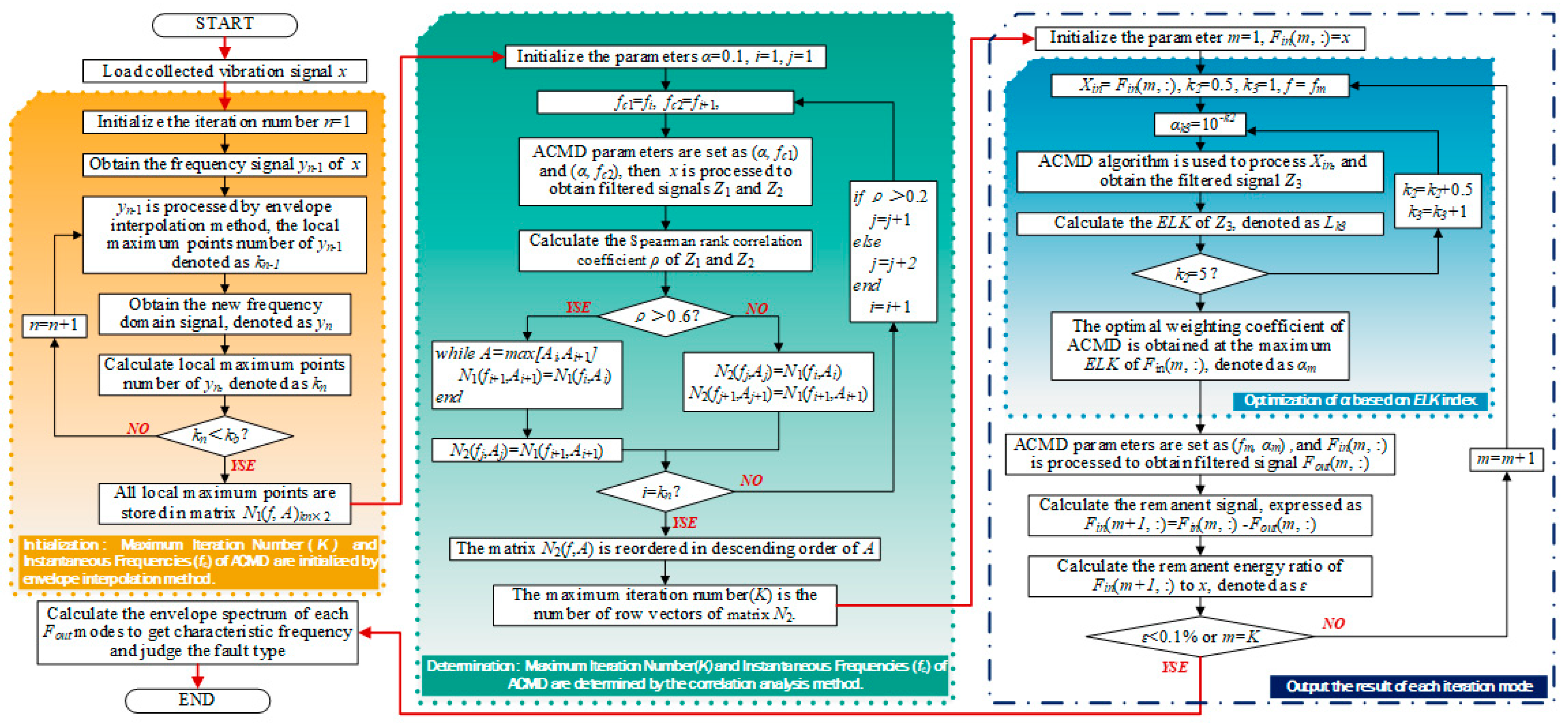
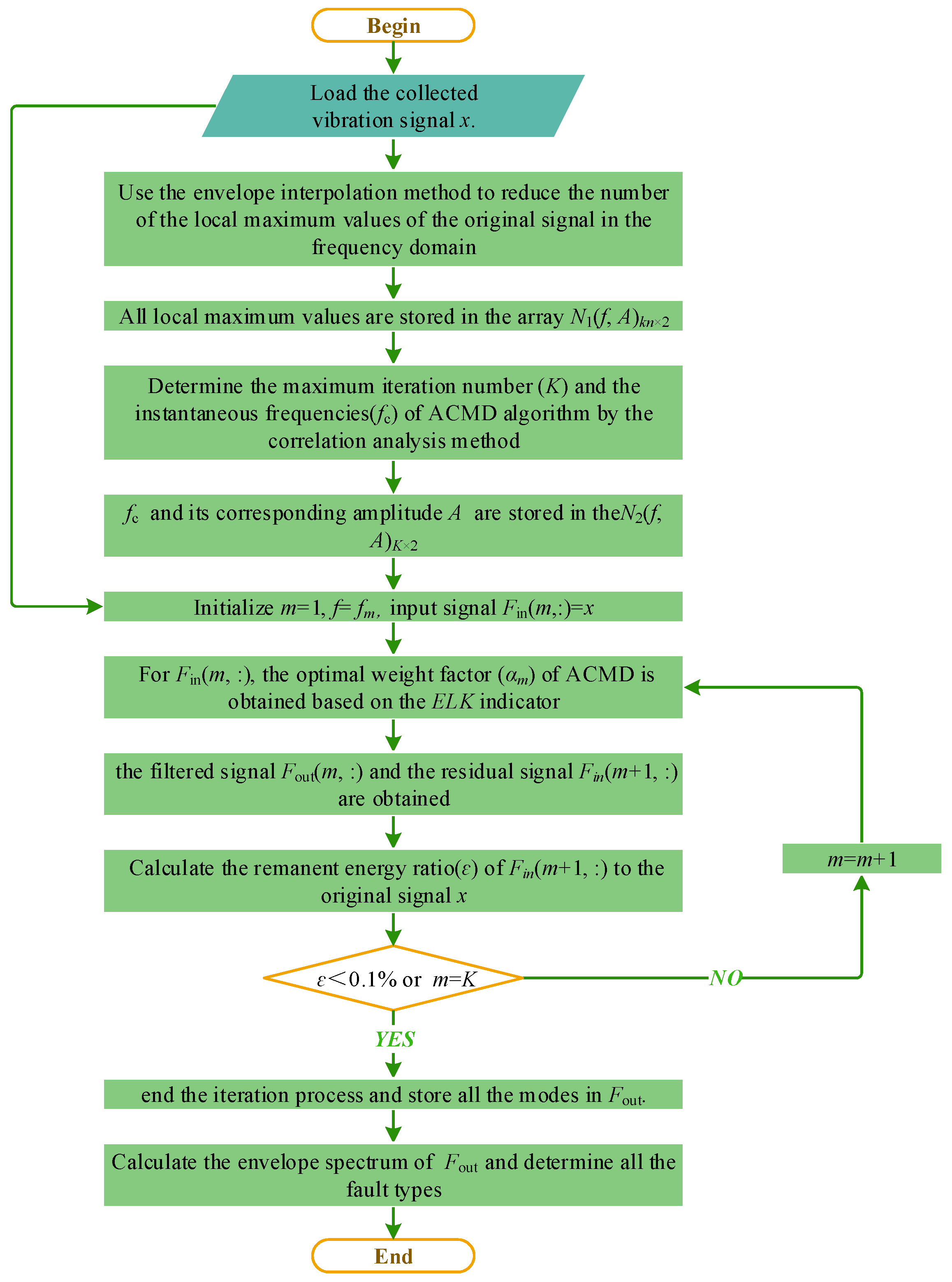
3. Proposed IMACMD Method

3.1. Overview of the Novel Iteration Fault Diagnostic Strategy

Bearing faults stimulate the resonance of the system. Theoretically, the fault characteristic signal is a narrow band signal with a specific excitation resonance frequency as its center frequency. However, in practice, the fault features are mixed with a lot of interference. As a direct fault feature extraction method, ACMD has some limitations. It is difficult to extract the fault information, especially for compound faults. It is also difficult to estimate the instantaneous frequency and the weight factor of ACMD accurately. Hence, in this paper, a novel iterative modified adaptive chirp mode decomposition (IMACMD) method is proposed to maximize the advantages of the ACMD algorithm. Firstly, the maximum iteration number (K) and the instantaneous frequency (fc) of each iteration are determined by envelope interpolation and similarity evaluation. Secondly, according to the input signal of each iteration, the weight factor (α) of the ACMD algorithm in each iteration is optimized adaptively and reasonably. Finally, the envelope spectra of the iteration filter signal are compared with the theoretical fault characteristic frequency to judge the fault types. The proposed IMACMD method is explained by the flowchart shown in Figure 6.

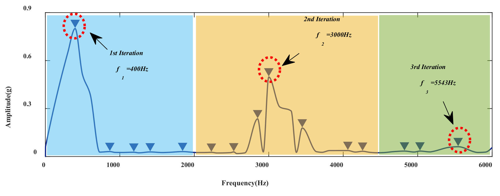
3.2. Determination of Maximum Iteration Number (K) and Instantaneous Frequencies (fc) of ACMD

3.2.1. Initialization

First, an envelope interpolation method is employed to preliminarily guide the potential instantaneous frequencies. It is applied to get the improved spectrum of the original signal by reducing the local maximum values and estimating the total fc close to the reasonable value. The process is illustrated in the yellow box in Figure 6. The detailed steps of this module can be summarized as follows:
(1) Load the collected vibration signal x.
(2) Initialize the iteration number n = 1.
(3) Obtain the frequency signal yn−1 of the original signal x.
(4) The number of the local maximum values of yn−1 is calculated and written as kn−1.
(5) yn−1 is processed by the interpolation envelop method, and the new frequency enveloped signal is denoted as yn.
(6) Calculate the number of the local maximum values of the obtained yn, written as kn.
(7) Judge whether kn < kb (kb is the boundary value, in default kb = 30). If no, n = n + 1 and repeat steps (5–7) until kn < kb. If yes, end the envelop interpolation process and output all the local maximum values that are stored in the matrix N1(f, A)kn×2, where f is the potential instantaneous frequency, A is the amplitude value of each local maximum, and kn is the initial maximum iteration number.
N 1 f , A = f 1 A 1 f k n A k n
Subsequent work in this section is further carried out to explain the reduction in the local maximum values through the simulated signal described in Section 2.3. The local maximum values in the spectrum of the original signal are represented by an inverted red triangle in Figure 7, with a total amount of 1330. However, the analysis result is unreasonable and not ideal because the spectrum contains too many details. Therefore, there is a need to reduce the number of extreme points.
After calculating the envelope of y0(t), the spherical spline interpolation method is used to solve the problem caused by the envelope. This interpolation method makes it easy to smooth the envelope line and further reduce the number of extreme points. In order to confirm the effect of the envelope interpolation method clearly, the results after each execution are shown in Figure 8. The first execution result is shown in Figure 8a, where the original envelope lines are smoothed, showing that the minor peaks of the original data sequence were abandoned.
As indicated in Figure 8b,c, after the second and third envelope and interpolation, the maximum values of the data sequence were greatly reduced. For the fourth time envelope displayed in Figure 8d, the detected local maximum values were reduced to 15. By applying this manipulation, the overall major local maximum values that stand for every local range could be recognized. However, if the number of executions was too large, the envelope line of the spectrum contained few local maximum values within a certain frequency range, or the envelope line ended up with a horizontal line.
In Figure 8e, only three local maximum values can be found within the fifth envelope line, and the important low-frequency maximum information between 0 and 1000 Hz was left out. Therefore, in order to avoid the loss of the typical global maximum values caused by too many iterations, a stop condition was set through kb (in default kb = 30). When the number of the local maximum values is less than kb, the envelope interpolation process is stopped. After four envelope interpolations of the simulated signal, the number of local maximum values was 15(<kb = 30), so the envelope stopped.

3.2.2. Adjustment

Even though the number of local maximum values decreased significantly through the multiple envelope and interpolation performance in Section 3.1, it would still be too redundant if each extremum point were iterated only once. As shown in the above envelope results of the simulating signals, using the ACMD algorithm to perform the iterative filtering for these 15 extreme points is cumbersome and unnecessary. Therefore, the correlation analysis method is employed to merge the extreme points with strong frequency correlation in N1(f, A), and the final iteration number and the instantaneous frequencies can be determined by the further reduced local maximum values. The updated K and fc are stored in N2(f, A). The process of the further adjustment is shown in Figure 6 (see the green box) and the detailed instructions are as follows:
(1) Load the matrix N1(f, A)kn×2.
(2) Initialize the parameters α = 0.1, i = 1, j = 1.
(3) fc1 = fi, fc2 = fi+1.
(4) ACMD parameters (α, fc1) and (α, fc2) are set, then the original signal x is processed to obtain the filtered signals Z1 and Z2.
(5) Calculate the Spearman rank correlation coefficient values of ρ for Z1 and Z2, respectively. The spearman coefficient [45] is a non-parametric index of the statistical dependence between two observational stochastic sequences. It accesses the relationship among the sequences in which the correlation coefficient can be depicted by using a monotonic function as:
ρ = 1 6 i = 1 n d i 2 q q 2 1
where d is the difference between the sequences, and q is the number of sequences. The correlation coefficient ρ > 0.6 is generally considered to be strongly relevant.
(6) Judge whether ρ > 0.6. If yes, the components with the smaller amplitudes in the frequency domain are discarded, whereas the components with the larger amplitudes are stored in the matrix N2(fj, Aj). Then j = j + 1, i = i + 1. If no, the information corresponding to the two frequency values is retained. N2(fj, Aj) = N1(fi, Ai), N2(fj+1, Aj+1) = N1(fi+1, Ai+1), j = j + 2 and i = i + 1.
(7) Judge whether i = kn. If yes, the maximum iteration number (K) is equal to the number of row vectors in the matrix N2(f, A), and then go to step 8. If no, repeat steps (3–7).
(8) The matrix N2(f, A)K×2 is rearranged in descending order of A so that the instantaneous frequency (fc) of each iteration can be determined.
Section 3.2 is used to process the matrix N1(f, A) obtained in Section 3.1, and the 15 maximum values are reduced to 3. After calculation, the five maximum values in the blue area in Figure 9 are the strongly correlated points, so only the maximum value with the highest amplitude is retained in the matrix N2(f1, A1) = (400, 0.800). Similarly, through correlation analysis, the yellow region and the green region can be found as the other two related regions, and the final results of the mergers are N2(f2, A2) = (3000, 0.497), N2(f3, A3) = (5543, 0.061). The maximum iteration number (K) is 3. As N2(f, A) reordered in the descending order of A, the instantaneous frequencies of ACMD for each iteration can be also determined.

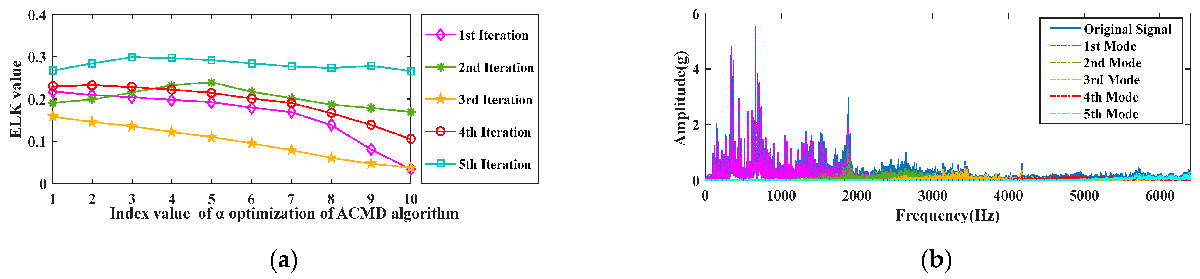
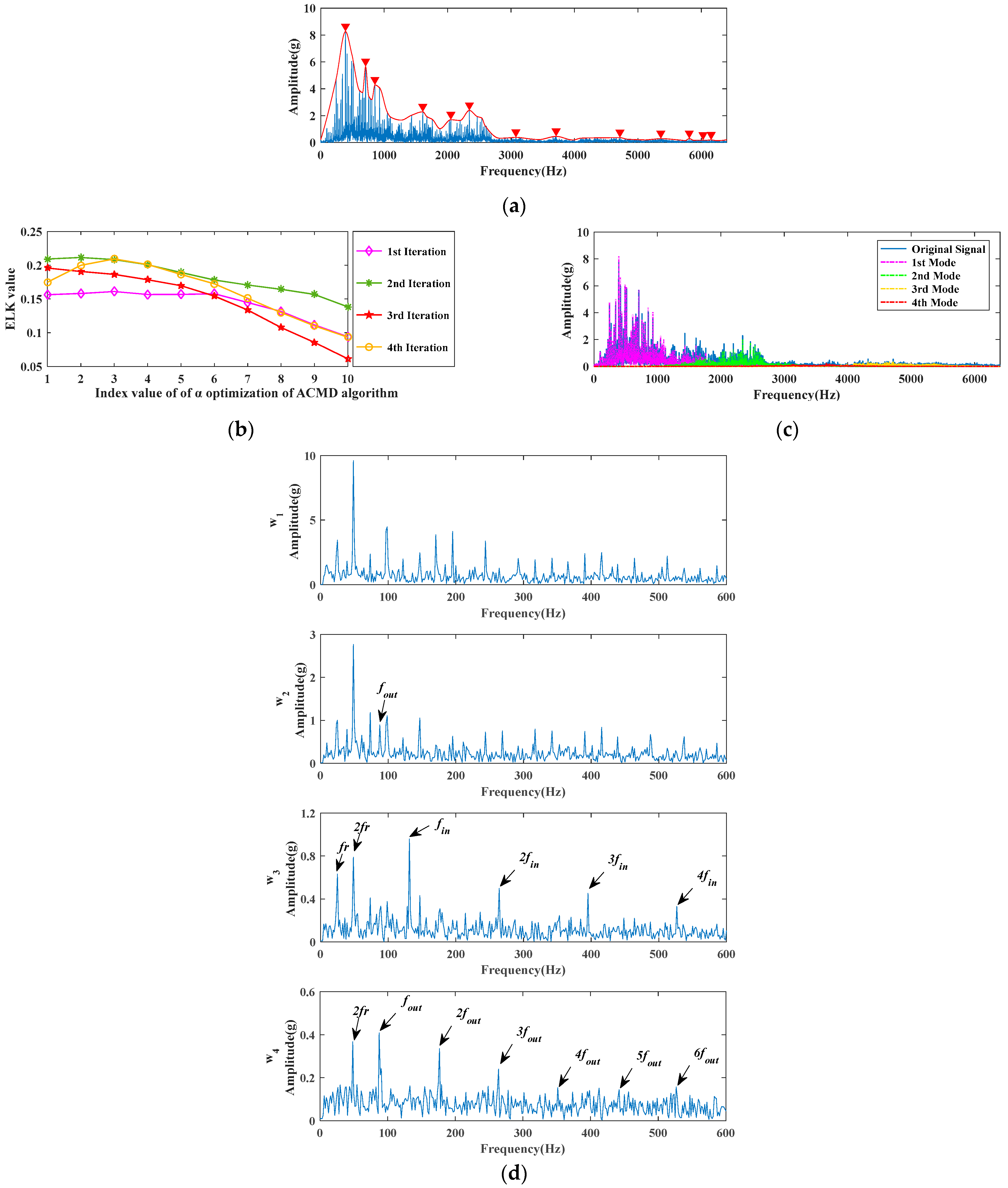
3.3. Weight Factor (α) Selection for ACMD

As mentioned, the selection of the weight factor (α) is also an important issue in ACMD. However, in rolling bearing signals, random impulses and harmonic components usually exist simultaneously. Consequently, different bandwidths should be provided to match each component. Additionally, in the actual signal, the energy of the random shocks, the harmonic components, and the noises is much more than that of the fault information. The aforementioned two points make it unreasonable to set a constant α to directly extract the fault information from the original signal or to progressively acquire the characteristic information of all the potential modes. Therefore, according to N2(f, A)K×2 obtained in Section 3.1, the complex components are separated step by step through the cyclic iteration. The optimization procedure of the parameter α for each component is shown in Figure 6 (see the blue box) and can be described as follows:
(1) Initialize the parameters k2 = 0.5, k3 = 1, f = fm. where fm is the instantaneous frequency obtained in Section 3.1.
(2) Calculate αk3 = 10k2.
(3) The parameters fc and αk3 of ACMD are set, and then the filtered signal Z3 can be obtained.
(4) Calculate the ELK of Z3, denoted as Lk3.
(5) Judge whether k2 = 5. If yes, go to step 6. If no, k2 = k2 + 0.5, k3 = k3 + 1, repeat steps (2–5).
(6) The α value corresponding to the maximum ELK is the optimal weight factor, which is denoted as αm.

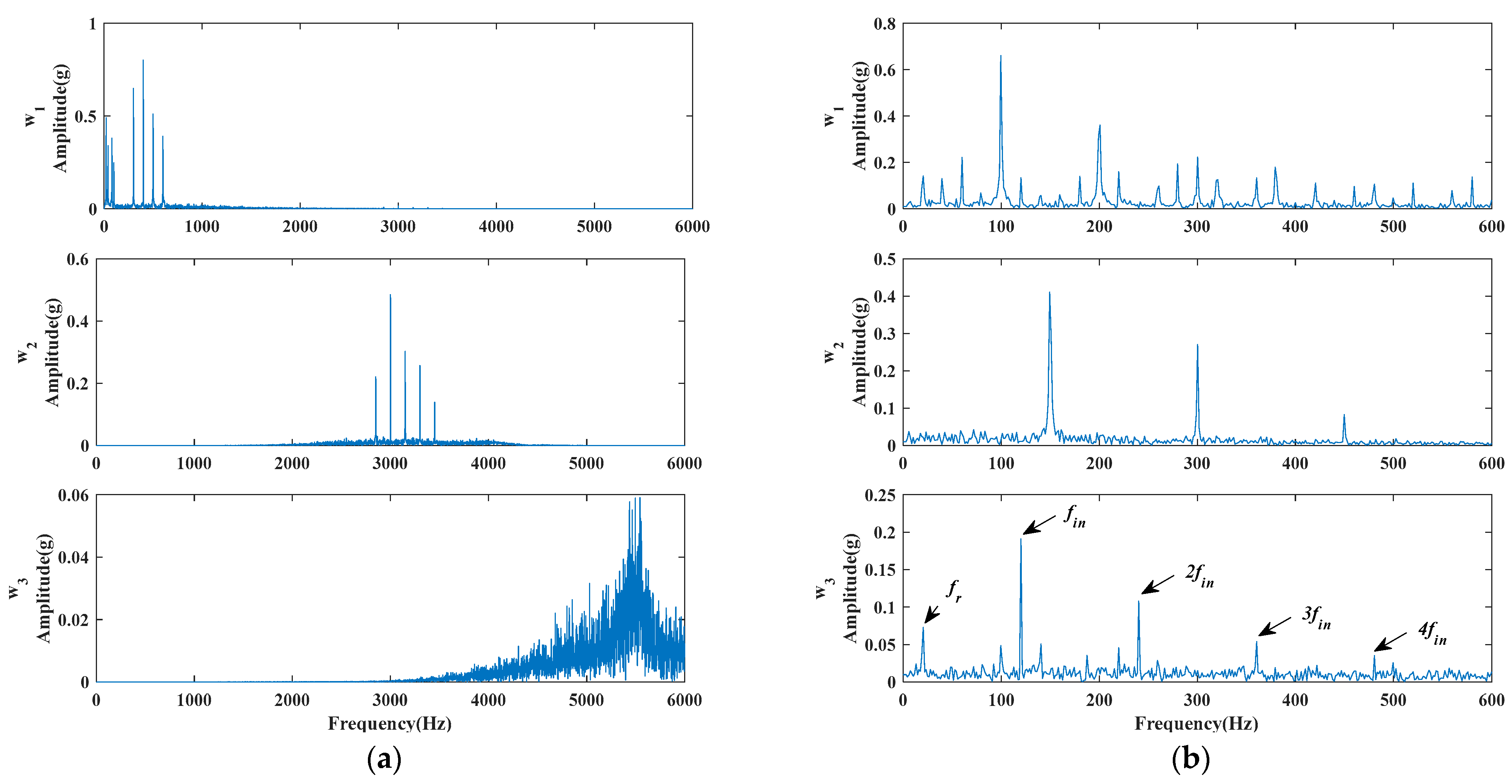
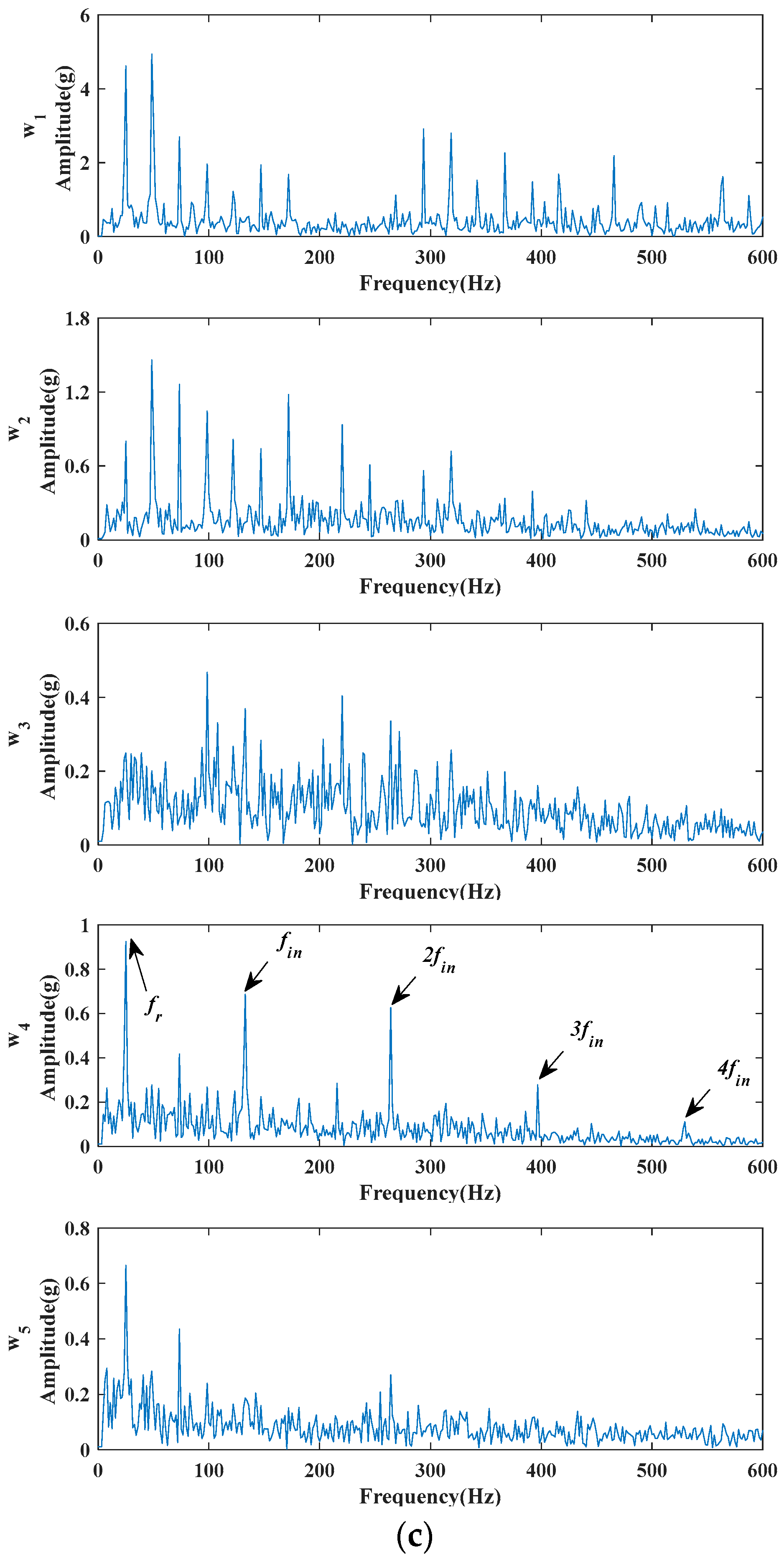
3.4. Feature Extraction Results of Each Iteration

The iteration output procedure is indicated in Figure 6 (see the dark blue dotted box) and can be summarized as follows:
(1) Load N2(f, A)K×2.
(2) Initialize the parameters m = 1, f = fm.
(3) Initialize the input signal of the iteration Fin(m, :) = x.
(4) As described in Section 3.2, calculate the ELK values with different α values in Fin(m, :). In this iteration, the optimal weight factor of ACMD is obtained at the largest ELK, denoted as αm.
(5) ACMD parameters fm and αm are set, and Fin(m, :) is processed to obtain the m-th filtered signal Fout(m, :).
(6) Calculate the remanent signal Fin(m + 1, :) = Fin(m, :)−Fout(m, :).
(7) Calculate the remanent energy ratio of Fin(m + 1, :) to the original signal x, denoted as
ε = F in 2 ( m + 1 , : ) x 2
(8) Judge whether ε < 0.1% and whether m = K. If yes, end the iteration process, and the filtered signals of m modes are stored in Fout. If no, m = m + 1 and repeat steps (4–8).
(9) Calculate the envelope spectra of the estimated m modes to determine whether the fault characteristic frequency of the bearing exists or not.
Similarly, taking the simulation signal as an example, x is further decomposed iteratively on the basis of N2(f, A). ELK values in different α cases for each Fin are calculated, as shown in Figure 10. Then the corresponding α(m) of each mode can be obtained.
The spectra of the three extracted target modes by ACMD with the instantaneous frequencies of 400 Hz, 3000 Hz, and 5543 Hz, respectively, are shown in the left column of Figure 11a. It is shown that the decomposition results were quite satisfactory because of the low correlation between each mode. The corresponding envelope spectra of the three extracted modes are displayed in the right column of Figure 11b. It can be found that the features of the different characteristic signals were successfully separated by the proposed method. The characteristic components of the rotating frequency (fr), the harmonic interference, and the inner race fault information (fin) are indicated in modes w1, w2, and w3, respectively. Based on the above analysis, it can be judged that the bearing had an inner race fault.

4. Application Procedures of the Proposed Method

The entire flowchart of the proposed IMACMD method is displayed in Figure 12, and the specific steps to apply the method for bearing fault diagnosis are given below:
Step 1: Load the collected vibration signal x.
Step 2: Use the envelope interpolation method to reduce the number of local maximum values of the original signal in the frequency domain. All local maximum values are stored in the array N1(f, A)kn×2.
Step 3: Determine the maximum iteration number (K) and the instantaneous frequencies (fc) of the ACMD algorithm by the correlation analysis method, denoted as N2(f, A)K×2.
Step 4: Initialize m = 1, f = fm, and input signal Fin(m, :) = x.
Step 5: For Fin(m, :), the optimal weight factor (αm) of ACMD is obtained based on the ELK indicator.
Step 6: Based on fm and αm, the filtered signal Fout(m, :) and the residual signal Fin(m + 1, :) are obtained.
Step 7: Calculate the remanent energy ratio (ε) of Fin(m + 1, :) to the original signal x.
Step 8: Judge whether ε < 0.1% or whether m = K. If yes, end the iteration process and store all the modes in Fout. Else, m = m + 1 and repeat steps (5–8).
Step 9: All the fault types are determined by the envelope spectrum of each mode.

5. Experimental Signal Verification

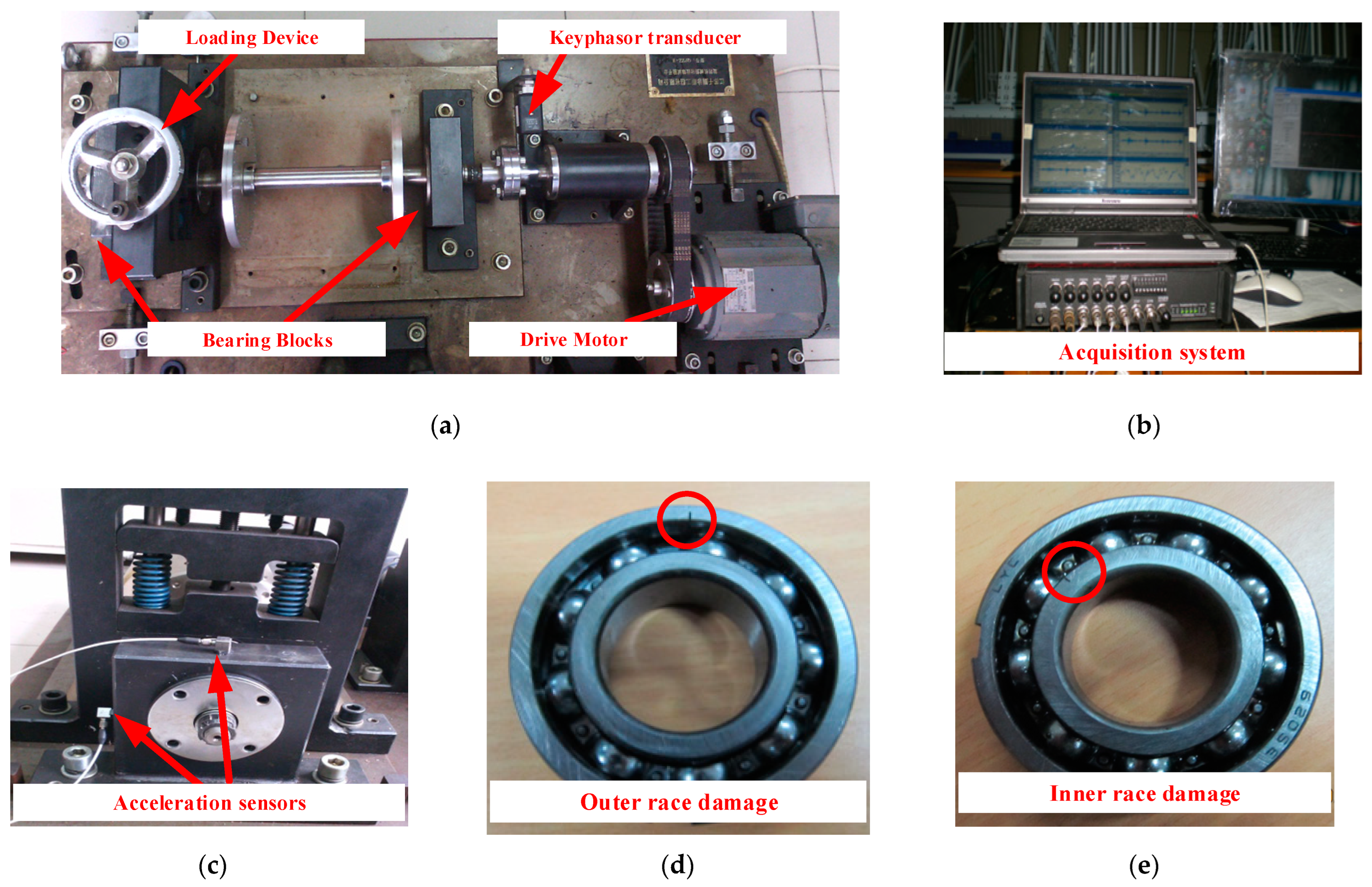
5.1. Experimental Setup Introduction

The effectiveness of the presented diagnostic frame was investigated by the vibration signals that were sampled from a QPZZ rotary machinery fault simulator. The details of the experimental fault simulator can be seen in Figure 13a. There was a loading device, an eddy current sensor, a drive motor, and several bearing blocks. As shown in Figure 13d,e, two of the same SKF6025 type bearings with an outer race and an inner race defect were used in the experiments. Electrical discharge machining was employed to produce a tiny groove on the races of the bearing. During the vibration signal measurement, the sampling frequency was set to 12,800 Hz. The rotating speed was set to 1470 rpm, with the rotating frequency set as fr = 24.5 Hz. According to the listed parameters of the SKF6205 bearings in Table 2, the theoretical fault characteristic frequencies of the inner race, the outer race, the roller, and the cage were calculated as fin = 132.67 Hz, fout = 87.83 Hz, froller = 115.48 Hz, and fcage = 9.76 Hz, respectively.

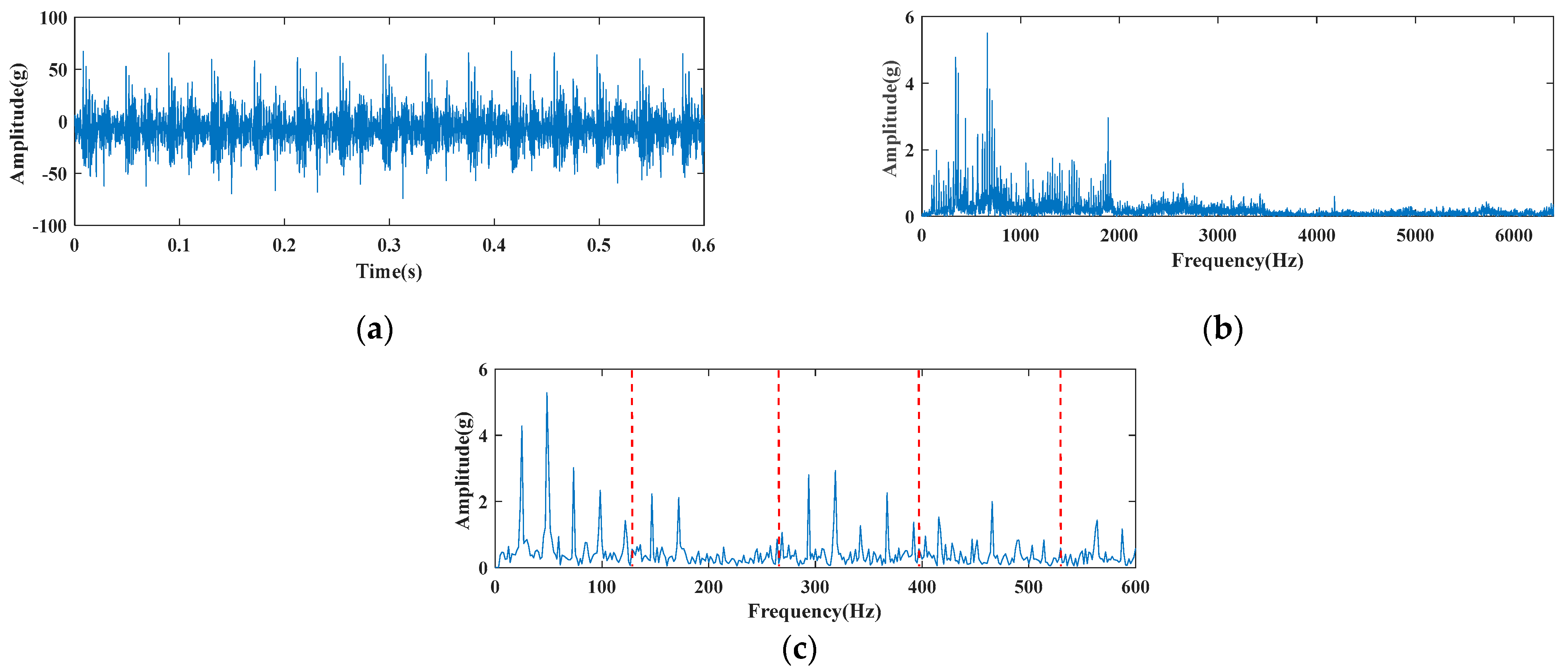
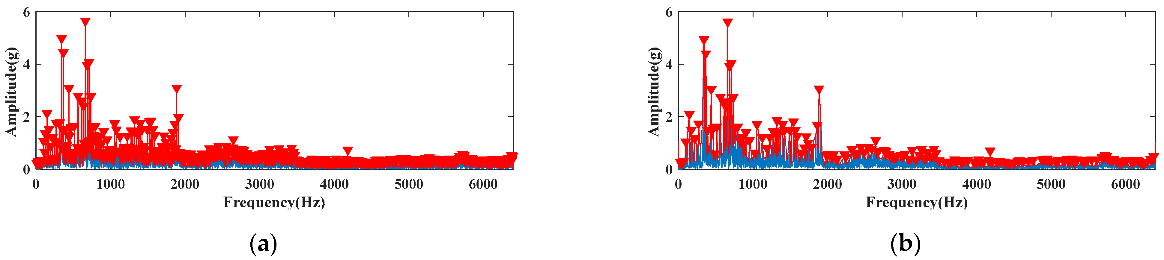
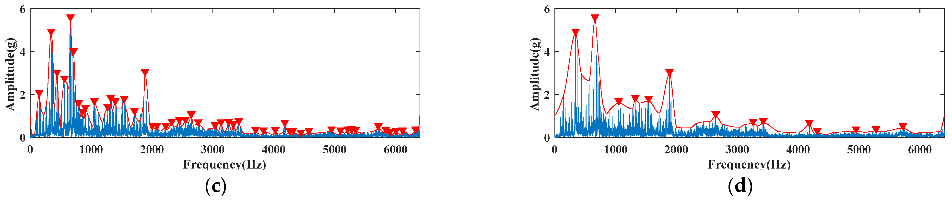
5.2. Single Fault Signal Analysis and Comparison

A dataset of the original inner race fault signal with 8192 points, whose frequency resolution and local stability were satisfied, was selected for the single fault analysis. In Figure 14a, some periodic impacts can be seen from the waveform of the experimental signal. However, the interval between two adjacent impacts was about 0.04 s, which corresponds to the shaft-rotating period.
The spectrum is shown in Figure 14b. It shows that the frequency components with high energy were mainly distributed below 3000 Hz, which means the resonance range was relatively wide. Moreover, the peak of 132.67 Hz, which was associated with the inner race defect, could not be observed. According to the envelope spectrum lines displayed in Figure 14c, no obvious spectral peaks could be found at the characteristic frequency of the inner race fault; see the red dotted line. On the contrary, the rotation frequency and its harmonics were obvious and in good accordance with the information in the time-domain waveform.
In the spectrum of the inner race fault signal, the number of local maximum values was 1304. As shown in Figure 15, the envelope interpolation method was performed four times on the original spectrum, and the local maximum values for each execution on the spectrum are marked by the red inverted triangles. It can be seen that the local maximum values after one, two, three, and four interpolations were 463, 156, 49, and 14, respectively.
According to the ACMD filtering effect on the local extremum points of different frequencies, the maximum values with strong correlation to the filtering results were reduced from 16 to 5, which is also the upper limit of the loop iteration. Therefore, the instantaneous frequencies of ACMD in each iteration were 661, 1886, 3259, 4313, and 5719, respectively. Based on the principle of the largest ELK, the optimal weight factor (α) of ACMD in each iteration was also captured, as shown in Figure 16a. Through the above optimization, the important parameters of the ACMD algorithm were set to complete the five time iterations. The inner race fault signal was decomposed into five modes, and the spectrum distribution is illustrated in Figure 16b. After processing by the IMACMD diagnosis method, the envelope spectrum of each mode is illustrated in Figure 16c, where the rotating frequency and its harmonics could be obviously found in modes w1 and w2, whereas the inner race fault feature frequency and its harmonics could be clearly observed in mode w4.
For comparison purpose, the widely used methods of singular spectrum decomposition (SSD) and spectral kurtosis (SK) were also applied to the experimental single fault signal.
SSD requests the mode decomposition quantitative parameters be preset in advance. In order to make the comparison results convincing, the number of singular spectrum components (SSC) was also set to 5, which is the output mode number of IMACMD. In Figure 17, the analysis results of SSD show that the inner race fault component had a very low amplitude and was only included in the envelope spectrum of SSC1. The rotating characteristics were widespread in all SSCs. These results show that SSD method was invalid for this experimental signal.
Then the experimental signal was processed by using the SK method. According to the SK kurtogram in Figure 18a, the optimal filtering frequency band was at level 5.5 and the center frequency was 2800 Hz. The envelope spectrum of the filtered signal by the constructed filter is displayed in Figure 18b. As indicated in Figure 18b, a lot of periodic impacts could be seen in the envelope spectrum, and their interval was about 24.5 Hz. Such an interval corresponds to the rotating frequency, but not the fault frequency.
Compared with the two widely used diagnosis methods, IMACMD obtained the most satisfying analysis results and had the advantage in the single bearing damage judgment.

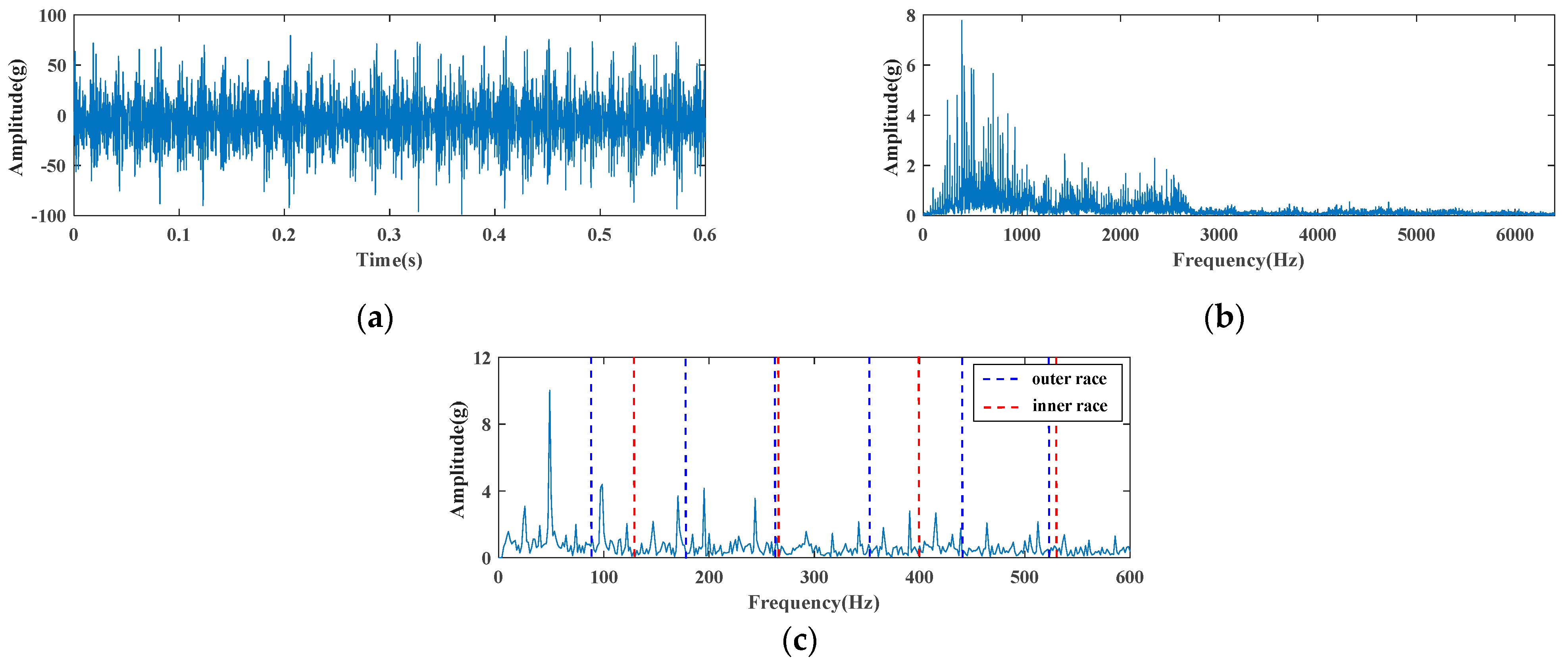
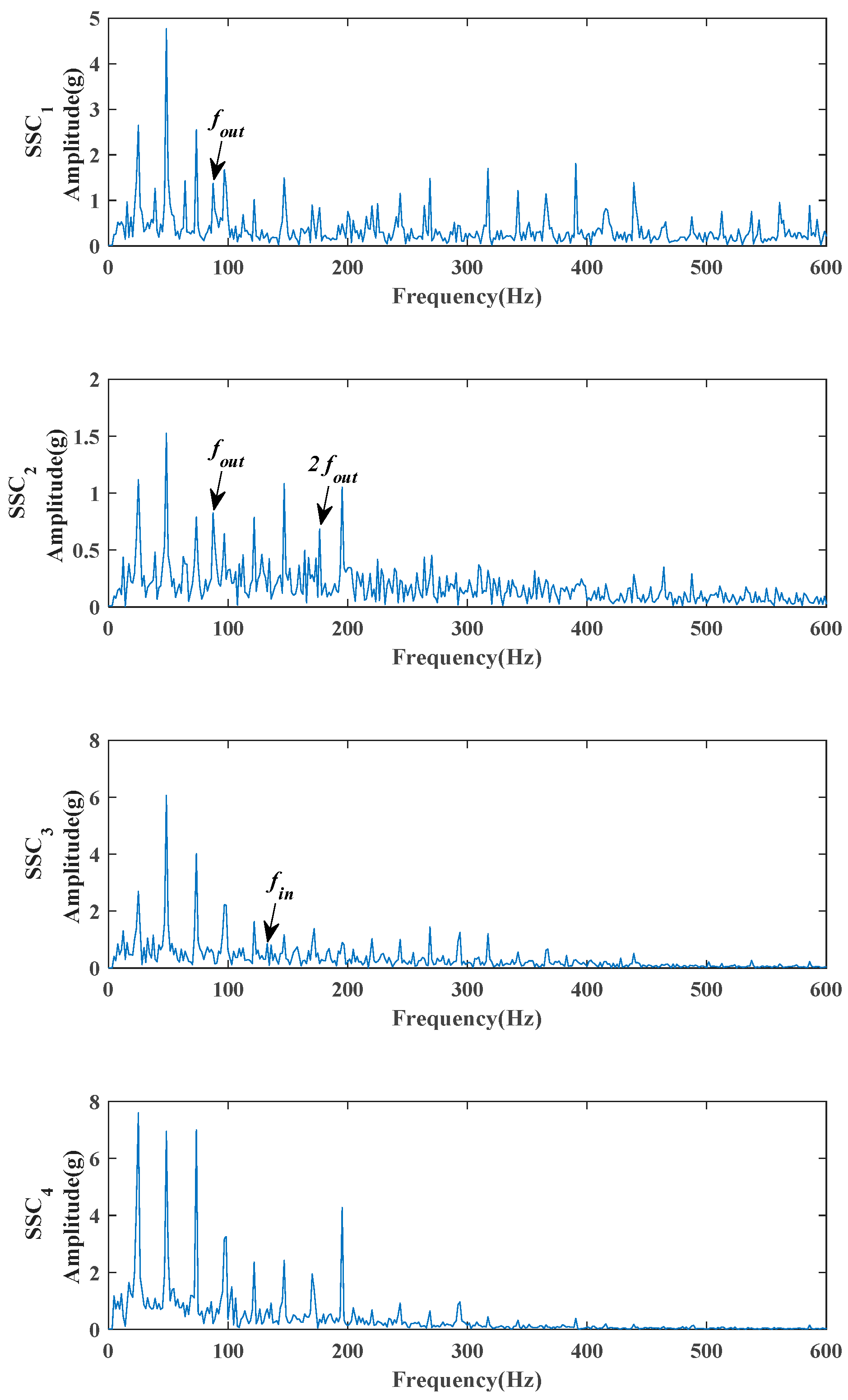
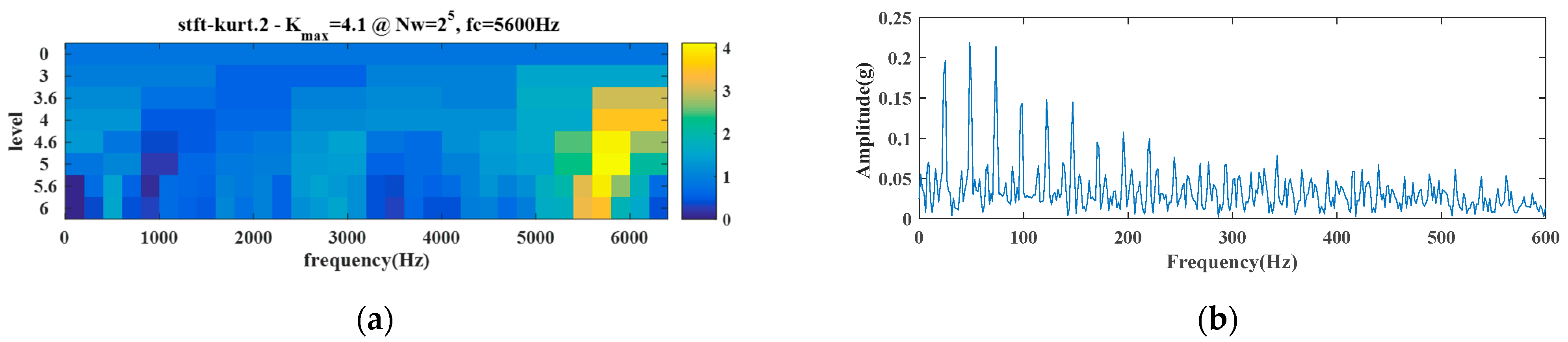
5.3. Compound Fault Signal Analysis and Comparison

In this subsection, the compound race fault was tested to further validate the superiority of the proposed IMACMD method. In Figure 19a, the observable impacts (about 0.02 s) corresponding to the harmonic components were associated with the rotating frequency. Such impact could also be obviously seen in the envelope spectrum in Figure 19c at 24.5 Hz. In Figure 19b, the energy concentration of the spectrum ranged from 0 Hz to 2500 Hz. In the envelope spectrum, the blue dotted line and the red dotted line represent the theoretical frequencies of the outer and the inner race faults, respectively. However, the bearing fault characteristic components of neither the inner nor the outer race fault were detected in the spectrum or the envelope spectrum; see Figure 19b,c.
Then the proposed diagnostic method was also employed in the analysis of the experimental compound fault signal, whose analysis results are displayed in Figure 20. By using the four-time envelope interpolation method, the estimated local maximum values of the spectrum were gradually reduced from the initial 1313 to the final 13, as shown in Figure 20a. By analyzing the similarity of the ACMD filter signals at each extremum point, the maximum iteration number was locked at 5, and meanwhile the instantaneous frequency of each iteration was also obtained, which was 391, 2344, 4717, 3711, and 5809, respectively. However, after the fourth iteration, the residual signal took up less than 0.1% energy of the original signal. It can be considered that the key information of the original signal had been extracted and the iteration ended. Therefore, through the dual constraints of the correlation analysis and the iteration end condition, the compound fault signal was eventually decomposed into four modes. According to Figure 20b, the optimal value of α for each iteration could be obtained. The spectrum distribution of each mode is illustrated in Figure 20c, whereas Figure 20d displays the envelope spectrums of the four separated modes. Modes w1 and w2 showed serial harmonics of fr, whereas the envelope spectrum of mode w3 revealed four harmonics of the inner race fault features. Particularly, the harmonics of the characteristic frequency fout~6fout could also be successfully detected through the envelope spectrum of w4. So far, the IMACMD method proposed in this paper successfully extracted and separated the inner and the outer race faults.
The number of SSCs was set to 4, and the compound fault signal analysis results of the SSD method are shown in Figure 21. Although the envelope spectra of SSC1 and SSC2 showed the fault characteristic frequency fout and the envelope spectrum of SSC3 displayed the fault characteristic frequency fin, the amplitude of the fault characteristic frequencies was quite low. At the same time, the harmonic interference of the rotating frequency was still serious. The fault features of both the inner and the outer race were extracted insufficiently, which means that the SSD method was invalid for handling this experimental compound fault signal.
The SK kurtogram for the compound fault signal analysis is displayed in Figure 22a, based on which the optimal frequency band was confirmed in level 5. Then the optimal filter with a center frequency of 6133.33 Hz was created to get the filtered signal. The corresponding envelope spectrum of the filtered signal is shown in Figure 22b. Obviously, it was easy to identify the harmonics of the rotating frequency at 24.5 Hz, whereas the fault characteristic frequencies of 132.67 Hz and 87.83 Hz could not be detected.
Therefore, for the composite fault signals, the acquired sensitive component using the IMACMD method could better separate the sensitive components and more effectively obtain the fault characteristics information than the SSD and SK methods.

6. Engineering Signal Verification

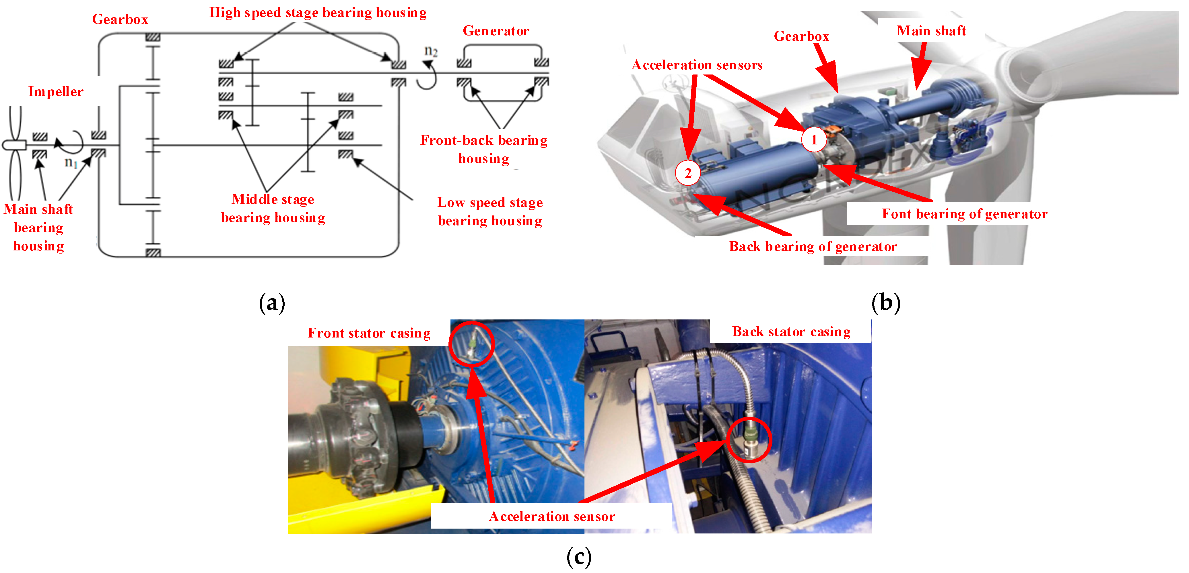
6.1. Wind Turbine Introduction

The proposed IMACMD diagnostic method was further validated through an actual bearing fault signal sampled from a 750 KW wind turbine generator. The schematic diagram of the wind turbine, which was composed of an impeller, a planetary gearbox, and a double-fed asynchronous generator, is illustrated in Figure 23a. The sensor positions are illustrated in Figure 23b, and the generator front–back stator casings are displayed in Figure 23.
Considering that the wind speed frequently varies in a random way, the rotating speed of the wind turbine consequently changes due to the mechanical torque/movement transfer. To validate the proposed method, we selected the data series that were sampled in a more stable wind speed condition, with a sampling frequency of 16,384 Hz. In the meantime, these long sampling data series were divided into several segments. Each segment was about 0.5 s, and within such short period the rotating speed of the wind turbine could be approximately treated as stable. The data segment employed for validation in this paper corresponded to a rotating speed of 1519 r/min.
The parameters of the defective SKF6324 bearing are listed in Table 3. In this practical engineering industrial equipment, local weak damage occurred on the outer race of the front generator bearing during the vibration monitoring. According to the structural details, the rotating frequency of the rotor fr = 25 Hz. Furthermore, the theoretical characteristic frequencies were also computed as fout = 79.2 Hz, fin = 123.2 Hz, froller = 110.9 Hz, and fcage = 15.4 Hz, respectively.

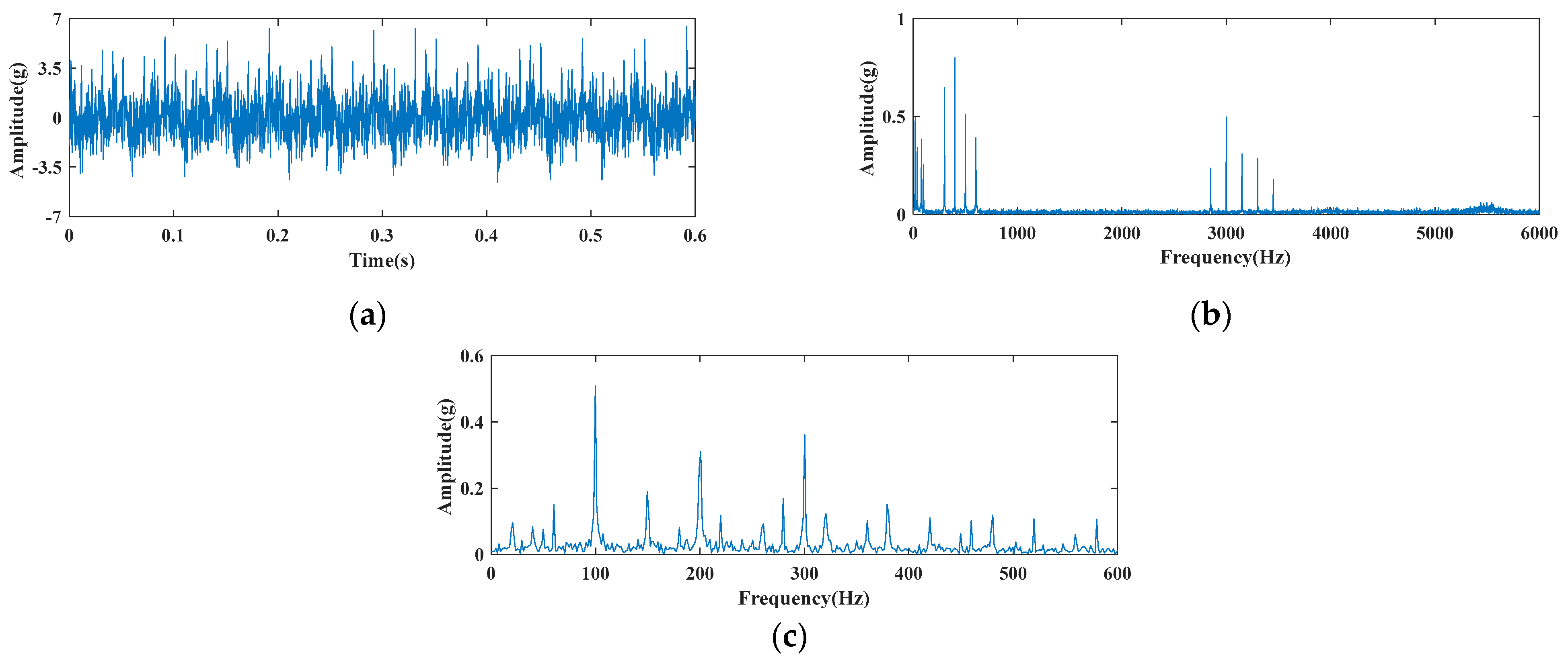
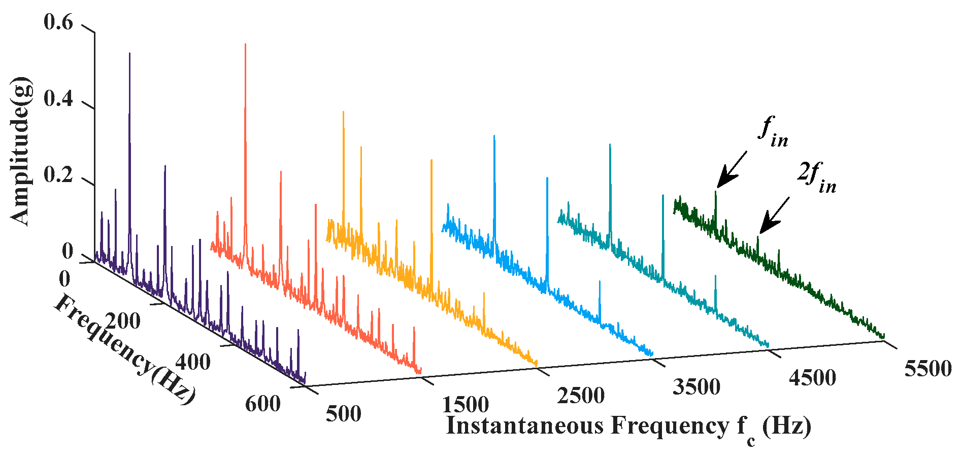
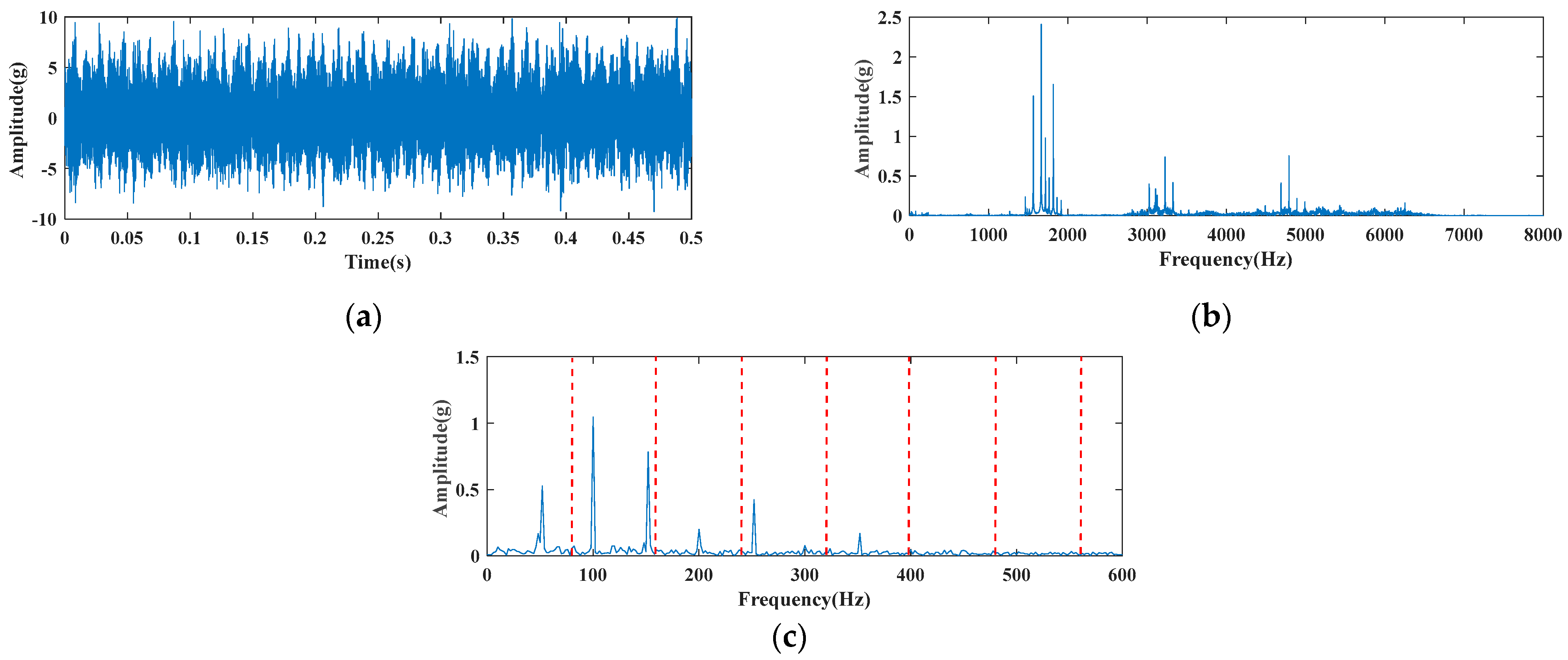
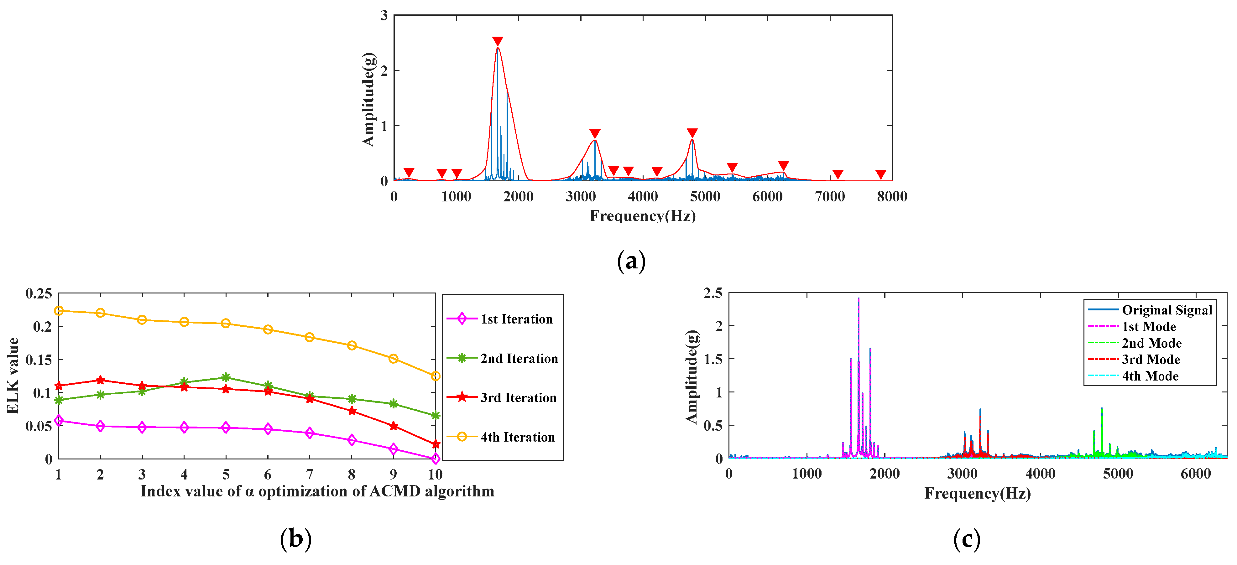
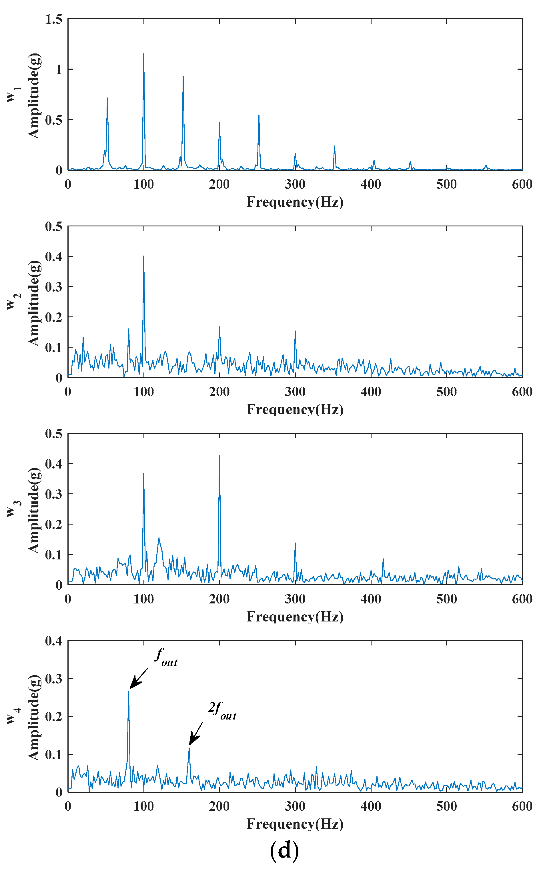
6.2. Engineering Signal Analysis and Comparison

As represented in Figure 24a, the impulsive phenomenon was unable to be observed from the waveform of this measured engineering signal with the data length of 8192 points. Figure 24b is the spectrum of the original signal, where there were only three significant frequency bands. Traditional envelope spectrum analysis was further performed on this vibration signal. In Figure 24c, the red dotted lines denote the fault frequency and its harmonics. Due to the harsh interference of the noise and the harmonics, only a rotating frequency of 25 Hz and its multiples were exhibited, whereas the fault characteristic frequency of the outer race could not be observed from the Hilbert envelope spectrum in Figure 24c. Thus, no diagnosis conclusion was able to be drawn based on the traditional analysis results.
To detect the bearing fault, the IMACMD method was employed to analyze the engineering signal. After four envelope interpolations, the local maximum values in the spectrum of the original signal were reduced from 1327 to 13, as shown in Figure 25a.
From Spearman rank correlation analysis, the modes with strong similarity were combined, and finally four effective local maximum values were left. By sorting the amplitudes of these extreme points, the instantaneous frequencies of the four iterations were 1664 Hz, 4797 Hz, 3226 Hz, and 6254 Hz, respectively. These four modes were defined as the primary ones to constitute the main information of the engineering signal. For each mode, the optimal value of αand the spectrum distribution are shown in Figure 25b,c. As illustrated in Figure 24, the envelope spectra of mode w1w3 contained some harmonics, whereas the envelope spectrum of mode w4 successfully separated the fault feature of the outer race.
To highlight the superiority of the proposed method, two different methods, i.e., SSD and SK, were also applied to analyze the actual engineering data for comparison.
By the SSD method, the engineering fault signal was decomposed into four components, and the envelope spectra of SSCs are illustrated in Figure 26. The characteristic frequency of the outer race fault had a smaller amplitude s to that in w4 in Figure 25d; hence, it could only be picked up in SSC1. Meanwhile, a lot of harmonics of the rotating frequency can be seen in SSC1, SSC2, and SSC3.
The comparison with SK is displayed in Figure 26. On the basis of the kurtogram information in Figure 27a, the optimal frequency bandwidth was at level 6 and the best center frequency was 6656 Hz. Then the envelope spectrum of the filtered signal could be presented, as shown in Figure 27b. It shows that only a feeble basic characteristic frequency was discovered, while its other harmonics were invisible. Obviously, the exhibited analysis of SK method was not as effective as that of IMACMD.
Through the previous engineering case analysis, an exact fault conclusion was unable to be drawn based on the analysis results of the SSD and SK methods. On the contrary, the proposed IMACMD method was more feasible and ascendant for weak fault feature extraction.

7. Conclusions

Strong noise removing and weak signal stripping from the vibration signal are crucial for bearing fault diagnosis, since in many cases the characteristics are often covered by heavy background noise. The ACMD method is a neoteric approach for adaptive signal processing and has a performance advantage in getting the target frequency characteristics. However, it is also greatly affected by some deficiencies. For instance, the detection of all the potential components and the key parameter setting needs prior knowledge. In this paper, a new iterative adaptive method, called IMACMD, is proposed to overcome these limitations. The contribution of this paper is as follows:
(1) As an iterative method, IMACMD can isolate all the modes from the original signal without the request of any prior knowledge about the rotation frequency, the fault frequency, etc. The proposed method is suitable for both single and compound fault signals, and the fault type can be identified successfully by the separated modes.
(2) The main advantage of IMACMD is using the dual constraints of the envelope interpolation as well as the Spearman rank correlation analysis to realize the minimization of the decomposition modes. Meanwhile, the instantaneous frequency parameters of each mode can be obtained.
(3) A new index named ELK is proposed in this paper, which is particularly effective for evaluating the degree of the periodicity from heavy noisy signals. Based on ELK index, the weight factor can be adaptively determined while extracting different mode components.
In the real datasets from experimental and engineering signals, the proposed method is superior to the SSD and SK methods in fault frequency detection, even though there is a variety of interferences from random impulses, large period fluctuations, and heavy noises. In this prospect, the proposed fault diagnosis method for rolling bearings has high potential to be widely applied, especially in multiple-fault and variable-speed cases.
In engineering, our method is qualified to diagnose both single and compound faults of bearings in approximately stable running conditions. However, in intensively varying speed cases, the proposed method is hard to use accurately. This issue will be investigated in future work.

Author Contributions

Conceptualization: G.T.; data curation: A.D.; investigation: A.D. and Y.H.; methodology: X.W.; software: S.F.; validation: Y.H.; writing—original draft: A.D.; writing—review and editing: Y.H. All authors have read and agreed to the published version of the manuscript.

Funding

The project is supported by the National Natural Science Foundation of China (grant No. 52005180); the Science and Technology Project of Hebei Education Department (grant No. QN2022190); the Natural Science Foundation of Hebei Province, China (grant No. E2022502003; No. E2020502031); and the Fundamental Research Funds for the Central Universities of China (grant No. 2021MS069).

Institutional Review Board Statement

Not applicable.

Informed Consent Statement

Not applicable.

Data Availability Statement

Not applicable.

Conflicts of Interest

The authors declare no conflict of interest.

Abbreviations

ACMDadaptive chirp mode decomposition
CYCBDcyclostationary blind deconvolution
EMDempirical mode decomposition
IMACMDiterative modified adaptive chirp mode decomposition
LMDlocal mean decomposition
MCKDmaximum correlated kurtosis deconvolution
MEDminimum entropy deconvolution
MOEDAmultipoint optimal minimum entropy deconvolution adjusted
SKspectral kurtosis
SSDsingular spectrum decomposition
SSCsingular spectrum component
VMDvariational mode decomposition
Notations
Aamplitude value of each local maximum
Anamplitude of cycle impacts
Bjamplitude of jth random impulse
Ckamplitude of kth harmonic component
ddifference between the sequences
ɛremanent energy ratio
fpotential instantaneous frequency
fcinstantaneous frequency
fcagecage fault characteristic frequency
fininner race fault characteristic frequency
fkresonance frequency of kth harmonic component
fmcoefficient of resonance frequency
fnresonance frequency of cycle impacts
foutouter race fault characteristic frequency
frrotating frequency
frollerroller fault characteristic frequency
fssampling frequency
fvresonance frequency of random impulses
Inumber of cycle impacts
Jnumber of random impulses
Kmaximum iteration number
kbboundary value of the local maximum
Kcnumber of harmonic components
knnumber of local maximum values
Nsampling points
qnumber of sequences
smimpulse response function of the rotating machinery system
ttime
Taperiod of cycle impacts
Tjoccurrence time of jth random impulse
wmode of IMACMD
αweight factor
βmcoefficient of resonance damping
γspecifies the slippage characteristic
μrrth L-moment
ρSpearman rank correlation coefficient values
φkphase of kth harmonic component
φmcoefficient of phase

References

  1. Cui, L.; Sun, Y.; Wang, X.; Wang, H. Spectrum-based, full-band preprocessing, and two-dimensional separation of bearing and gear compound faults diagnosis. IEEE Trans. Instrum. Meas. 2021, 70, 3513216. [Google Scholar] [CrossRef]
  2. Cheng, Z.; Wang, R. Enhanced symplectic characteristics mode decomposition method and its application in fault diagnosis of rolling bearing. Measurement 2020, 166, 108108. [Google Scholar] [CrossRef]
  3. Ma, J.; Zhuo, S.; Li, C.; Zhan, L.; Zhang, G. An enhanced intrinsic time-scale decomposition method based on adaptive lévy noise and its application in bearing fault diagnosis. Symmetry 2021, 13, 617. [Google Scholar] [CrossRef]
  4. Wang, T.; Chu, F.; Han, Q.; Kong, Y. Compound faults detection in gearbox via meshing resonance and spectral kurtosis methods. J. Sound Vib. 2017, 392, 367–381. [Google Scholar] [CrossRef]
  5. Guo, J.; Si, Z.; Xiang, J. A compound fault diagnosis method of rolling bearing based on wavelet scattering transform and improved soft threshold denoising algorithm. Measurement 2022, 196, 111276. [Google Scholar] [CrossRef]
  6. Hu, Y.; Zhou, Q.; Gao, J.; Li, J.; Xu, Y. Compound fault diagnosis of rolling bearings based on improved tunable Q-factor wavelet transform. Meas. Sci. Technol. 2021, 32, 105018. [Google Scholar] [CrossRef]
  7. Cao, H.; Su, S.; Jing, X.; Li, D. Vibration mechanism analysis for cylindrical roller bearings with single/multi defects and compound faults. Mech. Syst. Signal Process. 2020, 144, 106903. [Google Scholar] [CrossRef]
  8. Hu, Y.; Bao, W.; Tu, X.; Li, F.; Li, K. An adaptive spectral kurtosis method and its application to fault detection of rolling element bearings. IEEE Trans. Instrum. Meas. 2020, 69, 739–750. [Google Scholar] [CrossRef]
  9. Yang, B.; Lei, Y.; Jia, F.; Xing, S. An intelligent fault diagnosis approach based on transfer learning from laboratory bearings to locomotive bearings. Mech. Syst. Signal Process. 2019, 122, 692–706. [Google Scholar] [CrossRef]
  10. Meng, J.; Wang, H.; Zhao, L.; Yan, R. Compound fault diagnosis of rolling bearing using PWK-sparse denoising and periodicity filtering. Measurement 2021, 181, 109604. [Google Scholar] [CrossRef]
  11. Li, H.; Liu, T.; Wu, X.; Chen, Q.; Hua, L.; Tao, L.; Xing, W.; Qing, C. An enhanced frequency band entropy method for fault feature extraction of rolling element bearings. IEEE Trans. Ind. Inform. 2020, 16, 5780–5791. [Google Scholar] [CrossRef]
  12. Li, C.; Mo, L.; Yan, R. Fault diagnosis of rolling bearing based on WHVG and GCN. IEEE Trans. Instrum. Meas. 2021, 70, 3519811. [Google Scholar] [CrossRef]
  13. Yan, X.; Liu, Y.; Ding, P.; Jia, M. Fault diagnosis of rolling-element bearing using multiscale pattern gradient spectrum entropy coupled with Laplacian score. Complexity 2020, 2020, 4032628. [Google Scholar] [CrossRef]
  14. Cui, L.; Wang, X.; Wang, H.; Ma, J. Research on remaining useful life prediction of rolling element bearings based on time-varying Kalman filter. IEEE Trans. Instrum. Meas. 2020, 69, 2858–2867. [Google Scholar] [CrossRef]
  15. Luo, C.; Mo, Z.; Wang, J.; Jiang, J.; Dai, W.; Miao, Q. Multiple discolored cyclic harmonic ratio diagram based on meyer wavelet filters for rotating machine fault diagnosis. IEEE Sens. J. 2020, 20, 3132–3141. [Google Scholar] [CrossRef]
  16. Wang, T.; Han, Q.; Chu, F.; Feng, Z. A new SKRgram based demodulation technique for planet bearing fault detection. J. Sound Vib. 2016, 385, 330–349. [Google Scholar] [CrossRef]
  17. Antoni, J. The infogram: Entropic evidence of the signature of repetitive transients. Mech. Syst. Signal Process. 2016, 74, 73–94. [Google Scholar] [CrossRef]
  18. Moshrefzadeh, A.; Fasana, A. The Autogram: An effective approach for selecting the optimal demodulation band in rolling element bearings diagnosis. Mech. Syst. Signal Process. 2018, 105, 294–318. [Google Scholar] [CrossRef]
  19. Liu, Z.; Jin, Y.; Zuo, M.J.; Peng, D. Accugram: A novel approach based on classification to frequency band selection for rotating machinery fault diagnosis. ISA Trans. 2019, 95, 346–357. [Google Scholar] [CrossRef]
  20. Naima, G.; Elias, H.A.; Salah, S. An improved fast kurtogram based on an optimal wavelet coefficient for wind turbine gear fault detection. J. Electr. Eng. Technol. 2022, 17, 1335–1346. [Google Scholar] [CrossRef]
  21. Zhang, B.; Miao, Y.; Lin, J.; Yi, Y. Adaptive maximum second-order cyclostationarity blind deconvolution and its application for locomotive bearing fault diagnosis. Mech. Syst. Signal Process. 2021, 158, 107736. [Google Scholar] [CrossRef]
  22. Sen, D.; Long, J.; Sun, H.; Campman, X.; Buyukozturk, O. Multi-component deconvolution interferometry for data-driven prediction of seismic structural response. Eng. Struct. 2021, 241, 112405. [Google Scholar] [CrossRef]
  23. Luo, Y.; Cui, L.; Zhang, J.; Ma, J. Vibration mechanism and improved phenomenological model of the planetary gearbox with broken ring gear fault. J. Mech. Sci. Technol. 2021, 35, 1867–1879. [Google Scholar] [CrossRef]
  24. Cheng, Y.; Chen, B.; Zhang, W. Adaptive multipoint optimal minimum entropy deconvolution adjusted and application to fault diagnosis of rolling element bearings. IEEE Sens. J. 2019, 19, 12153–12164. [Google Scholar] [CrossRef]
  25. Wang, X.; Yan, X.; He, Y. Weak fault detection for wind turbine bearing based on ACYCBD and IESB. J. Mech. Sci. Technol. 2020, 34, 1399–1413. [Google Scholar] [CrossRef]
  26. Chen, B.; Zhang, W.; Song, D.; Cheng, Y. Blind deconvolution assisted with periodicity detection techniques and its application to bearing fault feature enhancement. Measurement 2020, 159, 107804. [Google Scholar] [CrossRef]
  27. Pang, B.; Nazari, M.; Tang, G. Recursive variational mode extraction and its application in rolling bearing fault diagnosis. Mech. Syst. Signal Process. 2022, 165, 108321. [Google Scholar] [CrossRef]
  28. Miao, Y.; Zhao, M.; Lin, J. Identification of mechanical compound-fault based on the improved parameter-adaptive variational mode decomposition. ISA Trans. 2019, 84, 82–95. [Google Scholar] [CrossRef]
  29. Peng, D.; Liu, Z.; Jin, Y.; Qin, Y. Improved EMD with a soft sifting stopping criterion and its application to fault diagnosis of rotating machinery. J. Mech. Eng. 2019, 55, 122–132. [Google Scholar] [CrossRef]
  30. Wang, L.; Liu, Z.; Miao, Q.; Zhang, X. Complete ensemble local mean decomposition with adaptive noise and its application to fault diagnosis for rolling bearings. Mech. Syst. Signal Process. 2018, 106, 24–39. [Google Scholar] [CrossRef]
  31. Wang, X.; Tang, G.; He, Y. Application of RSSD-OCYCBD strategy in enhanced fault detection of rolling bearing. Complexity 2020, 2020, 5424236. [Google Scholar] [CrossRef]
  32. Wang, R.; Xu, L.; Liu, F. Bearing fault diagnosis based on improved VMD and DCNN. J. Vibroeng. 2020, 22, 1055–1068. [Google Scholar] [CrossRef]
  33. Huang, W.; Li, N.; Selesnick, I.; Shi, J.; Wang, J.; Mao, L.; Jiang, X.; Zhu, Z. Nonconvex group sparsity signal decomposition via convex optimization for bearing fault diagnosis. IEEE Trans. Instrum. Meas. 2019, 69, 4863–4872. [Google Scholar] [CrossRef]
  34. Wang, X.; He, Y.; Wang, H.; Hu, A.; Zhang, X. A novel hybrid approach for damage identification of wind turbine bearing under variable speed condition. Mech. Mach. Theory 2022, 169, 104629. [Google Scholar] [CrossRef]
  35. Chen, S.; Dong, X.; Peng, Z.; Zhang, W.; Meng, G. Nonlinear chirp mode decomposition: A variational method. IEEE Trans. Signal Process. 2017, 65, 6024–6037. [Google Scholar] [CrossRef]
  36. Chen, S.; Yang, Y.; Peng, Z.; Wang, S.; Zhang, W.; Chen, X. Detection of rub-impact fault for rotor-stator systems: A novel method based on adaptive chirp mode decomposition. J. Sound Vib. 2019, 440, 83–99. [Google Scholar] [CrossRef]
  37. Ma, Z.; Lu, F.; Liu, S.; Li, X. A parameter-adaptive ACMD method based on particle swarm optimization algorithm for rolling bearing fault diagnosis under variable speed. J. Mech. Sci. Technol. 2021, 35, 1851–1865. [Google Scholar] [CrossRef]
  38. Liu, Q.; Wang, Y.; Wang, X. Two-step Adaptive Chirp Mode Decomposition for time-varying bearing fault diagnosis. IEEE Trans. Instrum. Meas. 2021, 70, 3055291. [Google Scholar] [CrossRef]
  39. Wang, X.; Tang, G.; Yan, X.; He, Y.; Zhang, X.; Zhang, C. Fault diagnosis of wind turbine bearing based on optimized Adaptive Chirp Mode Decomposition. IEEE Sens. J. 2021, 21, 13649–13666. [Google Scholar] [CrossRef]
  40. Chen, S.; Yang, Y.; Peng, Z.; Dong, X.; Zhang, W.; Meng, G. Adaptive chirp mode pursuit: Algorithm and applications. Mech. Syst. Signal Process. 2019, 116, 566–584. [Google Scholar] [CrossRef]
  41. Yang, Q.; Ruan, J.; Zhuang, Z. Fault diagnosis for circuit-breakers using adaptive chirp mode decomposition and attractor’s morphological characteristics. Mech. Syst. Signal Process. 2020, 145, 106921. [Google Scholar] [CrossRef]
  42. Liang, K.; Zhao, M.; Lin, J.; Ding, C.; Jiao, J.; Zhang, Z. A novel indicator to improve fast kurtogram for the health monitoring of rolling bearing. IEEE Sens. J. 2020, 20, 12252–12261. [Google Scholar] [CrossRef]
  43. Bao, W.; Tu, X.; Hu, Y.; Li, F. Envelope spectrum L-Kurtosis and its application for fault detection of rolling element bearings. IEEE Trans. Instrum. Meas. 2020, 69, 1993–2002. [Google Scholar] [CrossRef]
  44. Gao, Q.; Xiang, J.; Hou, S.; Tang, H.; Zhong, Y.; Ye, S. Method using L-Kurtosis and enhanced clustering-based segmentation to detect faults in axial piston pumps. Mech. Syst. Signal Process. 2021, 147, 107130. [Google Scholar] [CrossRef]
  45. Song, H.Y.; Park, S. An analysis of correlation between personality and visiting place using Spearman’s rank correlation coefficient. KSII Trans. Internet Inf. Syst. 2020, 14, 1951–1966. [Google Scholar]
Figure 1. Components of the simulated signal: (a) fault feature signal; (b) random impulses; (c) harmonic components; (d) white noise.
Machines 10 00704 g001
Figure 2. Comparison of the four indexes.
Machines 10 00704 g002
Figure 3. Simulated signal: (a) waveform; (b) frequency spectrum; (c) envelope spectrum.
Machines 10 00704 g003
Figure 4. The envelope spectrums of filtering signals by ACMD with different fc.
Machines 10 00704 g004
Figure 5. Filtering signals by ACMD with different α: (a) envelope spectrums; (b) ELK value.
Machines 10 00704 g005
Figure 6. Implementation steps of the proposed IMACMD.
Machines 10 00704 g006
Figure 7. The local maximum values in the frequency spectrum of the original signal.
Machines 10 00704 g007
Figure 8. Envelope interpolation process: (a) 1st time execution; (b) 2nd time execution; (c) 3rd time execution; (d) 4th time execution; (e) 5th time execution.
Machines 10 00704 g008
Figure 9. Adjustment process.
Machines 10 00704 g009
Figure 10. ELK values with different α at each Fin.
Machines 10 00704 g010
Figure 11. Analysis results of each mode of the simulated inner race fault signal: (a) frequency spectrum; (b) envelope spectrum.
Machines 10 00704 g011
Figure 12. Fault diagnosis steps based on the proposed IMACMD method.
Machines 10 00704 g012
Figure 13. The local machinery fault simulator: (a) The experimental fault simulation operation platform; (b) signal acquisition display; (c) acceleration sensor locations; (d) outer race fault bearing; (e) inner race fault bearing.
Machines 10 00704 g013
Figure 14. Experimental signal of bearing inner race single fault: (a) waveform; (b) frequency spectrum; (c) envelope spectrum.
Machines 10 00704 g014
Figure 15. The envelope interpolation method process of experimental inner race failure signal: (a) 1st time execution; (b) 2nd time execution; (c) 3rd time execution; (d) 4th time execution.
Machines 10 00704 g015aMachines 10 00704 g015b
Figure 16. Proposed diagnostic strategy analysis results of experimental inner race fault signal: (a) ELK values with different α at each Fin; (b) frequency spectrum distribution results of the obtained modes; (c) envelope spectrums of the obtained modes.
Machines 10 00704 g016aMachines 10 00704 g016b
Figure 17. SSD decomposing results of the experimental inner race fault signal.
Machines 10 00704 g017
Figure 18. SK filtering result of experimental inner race fault signal: (a) kurtogram; (b) envelope spectrum of the filtered signal.
Machines 10 00704 g018
Figure 19. Experimental signal of bearing races compound fault: (a) waveform; (b) frequency spectrum; (c) envelope spectrum.
Machines 10 00704 g019
Figure 20. Proposed diagnostic strategy analysis results of experimental compound fault signal: (a) envelope and interpolation results; (b) ELK values with different α at each Fin; (c) frequency spectrum distribution results of the obtained modes; (d) envelope spectrums of the obtained modes.
Machines 10 00704 g020
Figure 21. SSD decomposing results of the experimental compound fault signal.
Machines 10 00704 g021
Figure 22. SK analysis results of experimental compound fault signal: (a) kurtogram; (b) envelope spectrum of the filtered signal.
Machines 10 00704 g022
Figure 23. Wind turbine: (a) schematic diagram; (b) accelerometers positions; (c) front-stator casing and back-stator casing.
Machines 10 00704 g023
Figure 24. Engineering fault signal: (a) waveform; (b) frequency spectrum; (c) envelope spectrum.
Machines 10 00704 g024
Figure 25. Proposed diagnostic strategy analysis results of engineering fault signal: (a) envelope and interpolation results; (b) ELK values with different α at each Fin; (c) spectrum distribution results of the obtained modes; (d) envelope spectrums of the obtained modes.
Machines 10 00704 g025aMachines 10 00704 g025b
Figure 26. SSD decomposing results of the engineering fault signal.
Machines 10 00704 g026
Figure 27. SK analysis results of the engineering fault signal: (a) kurtogram; (b) envelope spectrum of the filtered signal.
Machines 10 00704 g027
Table 1. Setting of the simulated signal.
ParameterMeaningValue
Fault feature signal
INumber of cycle impacts165
AAmplitude of cycle impacts1.1
fnResonance frequency of cycle impacts5500 Hz
TaPeriod of cycle impacts0.0083 s
γSpecifies the slippage characteristicrandom value in 1–2% Ta
Random impulses
JNumber of random impulses3
B1, B2, B3Amplitude of jth random impulse2, 3, 4
fvResonance frequency of random impulses4000 Hz
T1, T2, T3Occurrence time of jth random impulse0.08 s, 0.20 s, 0.25 s
Harmonic components
KNumber of harmonic components8
C1C8Amplitude of kth harmonic component0.7, 0.8, 0.6, 0.5
0.3, 0.5, 0.4, 0.3
f1f8Resonance frequency of kth harmonic component300, 400, 500, 600,
2850, 3000, 3150, 3300
φkPhase of kth harmonic componentπ/2
Table 2. Parameters of the SKF6205 bearing.
Ball NumberBall DiameterPitch DiameterContact Angle
97.94 mm39.04 mm
Table 3. Parameters of the SKF6324 bearing.
Ball NumberBall DiameterPitch DiameterContact Angle
841.275 mm190 mm
Publisher’s Note: MDPI stays neutral with regard to jurisdictional claims in published maps and institutional affiliations.

