
Adaptive Band Extraction Based on Low Rank Approximated Nonnegative Tucker Decomposition for Anti-Friction Bearing Faults Diagnosis Using Measured Vibration Data


Abstract
:1. Introduction
- (1)
- For CPD, the rank-one decomposition property requires the same number of lower ranks for each tensor mode (the dimensions of a tensor are often referred to as modes), which might be incompatible to express the inherent correlations where each mode has various number of latent components;
- (2)
- Although different low-rank dimensions are allowed, the Tucker decomposition is often criticized for its poor uniqueness and the curse of dimensionality (i.e., the core tensor is dense whose entry number scales exponentially with the tensor order) [30];
- (3)
- Diverse ways of representing vibration data as tensors can be found while a physically interpretable way is needed. To this end, the multi-dimensional correlation across different modes (such as the spectral, temporal, and spatial modes) might need more intuitive illustrations for diagnostic purposes.
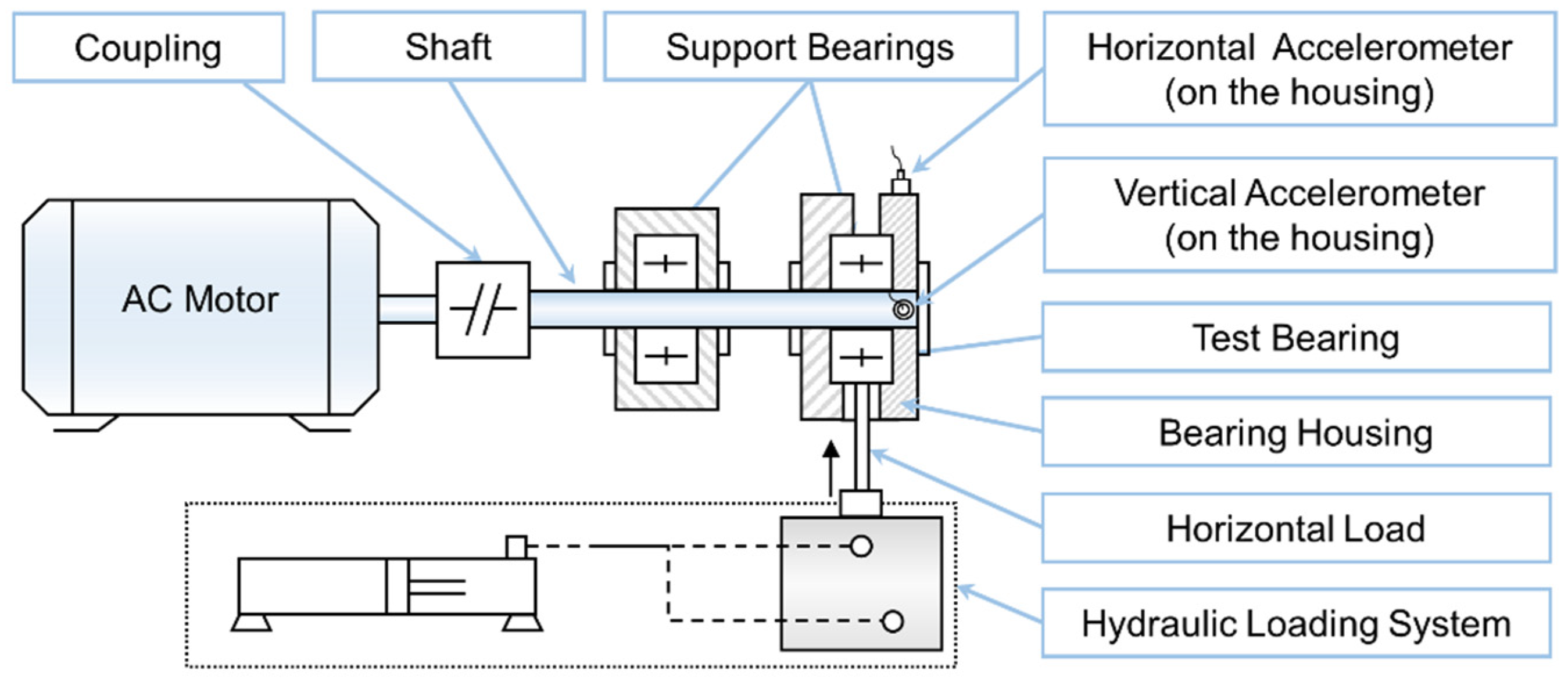
2. Experimental Rig and Measured Vibration
3. Proposed Method
3.1. Nonnegative Tucker Decomposition Based on Low-Rank Approximation
3.1.1. Standard Nonnegative Tucker Decomposition (NTD)
3.1.2. The Low Rank Approximated NTD (LRANTD) Model
- (1)
- LRA. Perform unconstrained Tucker decomposition as in (1) using HOSVD to obtain an approximation of the original tensor, , which givesand the mode- unfolding of the LRA tensor, ,
- (2)
- NTD. Minimize the new cost functions with the nonnegativity constraints on the factors as in (8). Note that given the tensor order , a total of unfolding forms from are defined in (7) and the sequence of minimization problems should be calculated for each factor matrix, .
3.1.3. Optimization Algorithms
- The iterative update rule for mode- (factor) matrices
- The iterative update rule for core tensor
3.2. Diagnostic Scope of the LRANTD Model
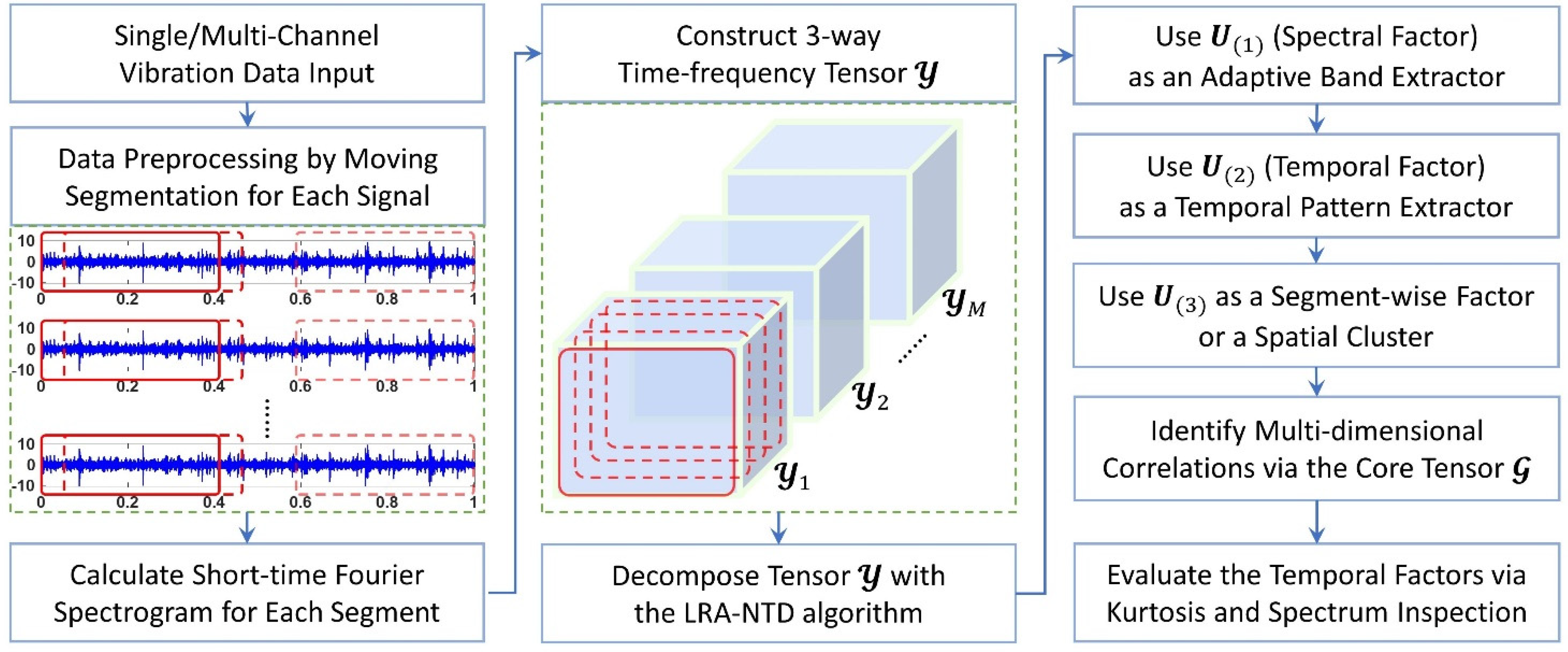
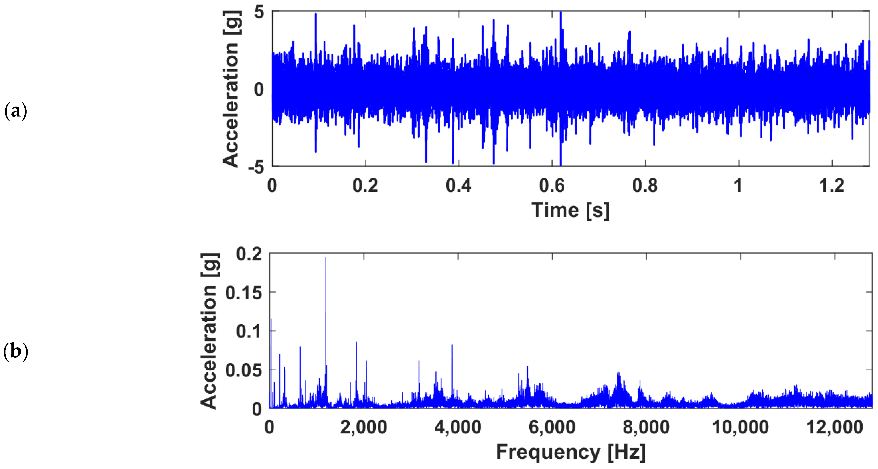
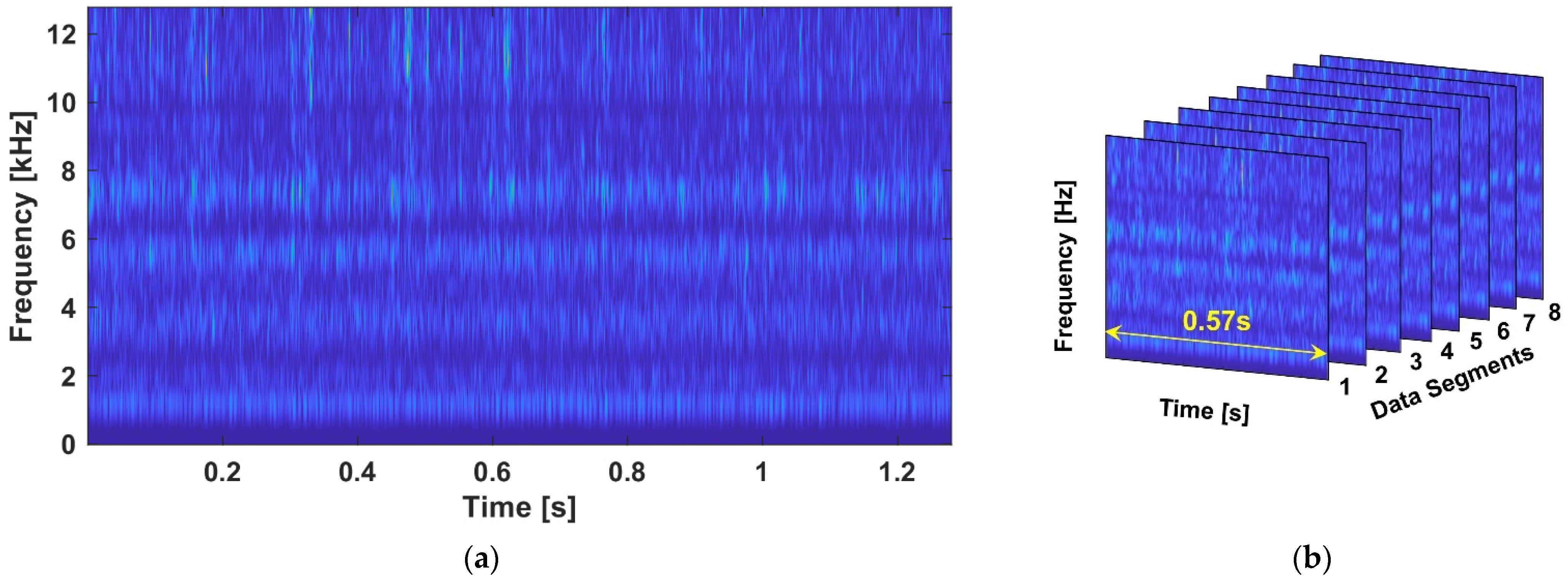
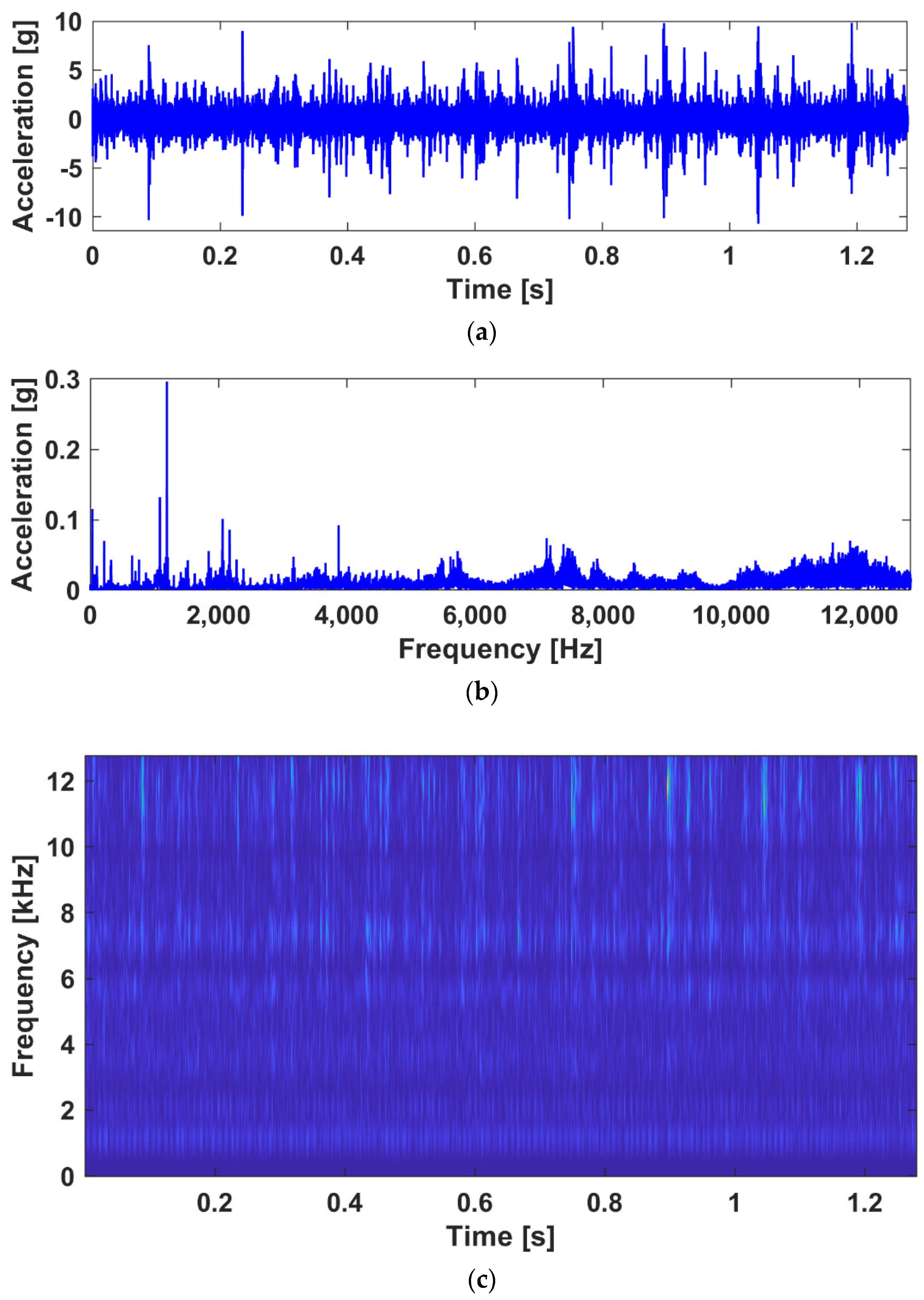
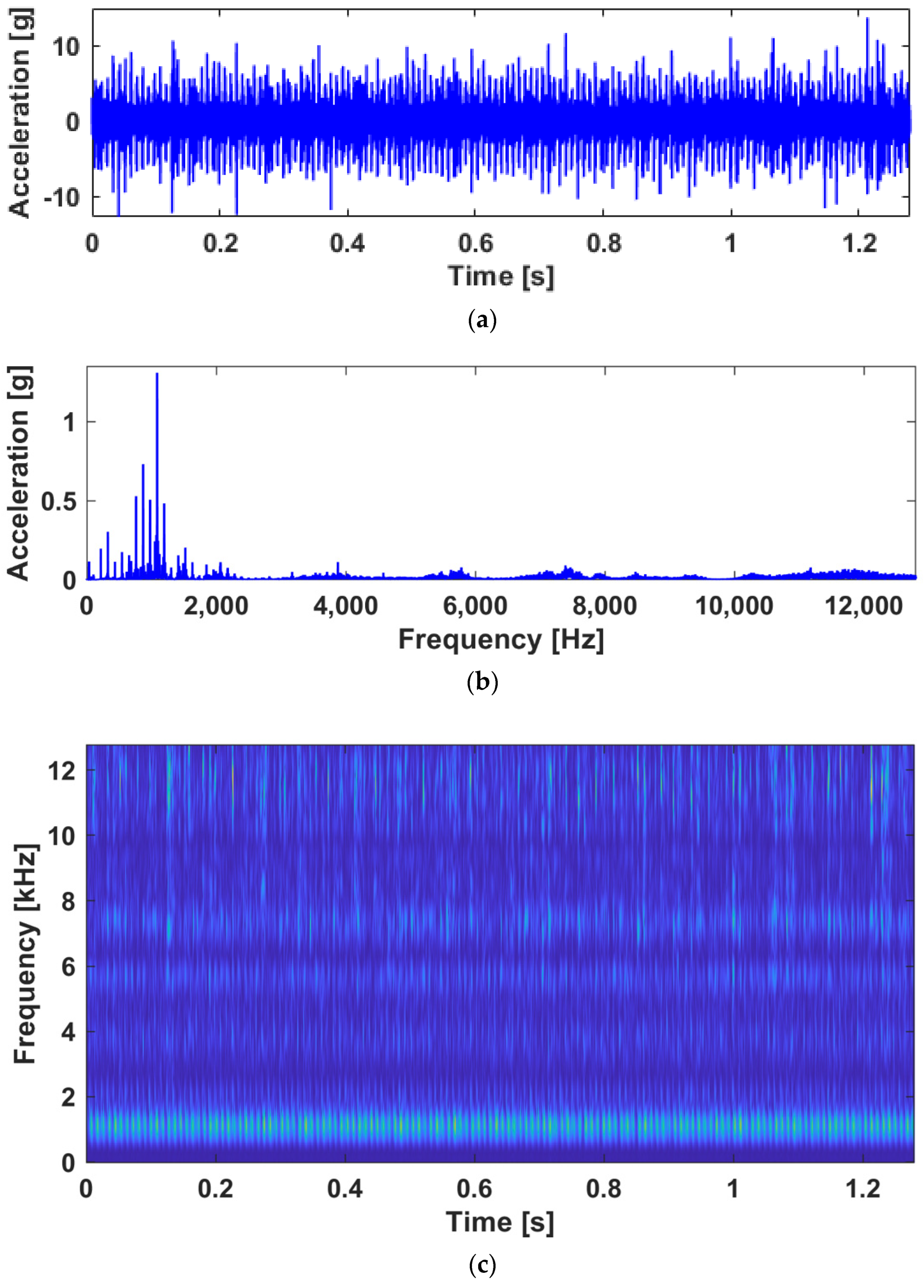
3.2.1. Data Pre-Processing: Moving Segmentation
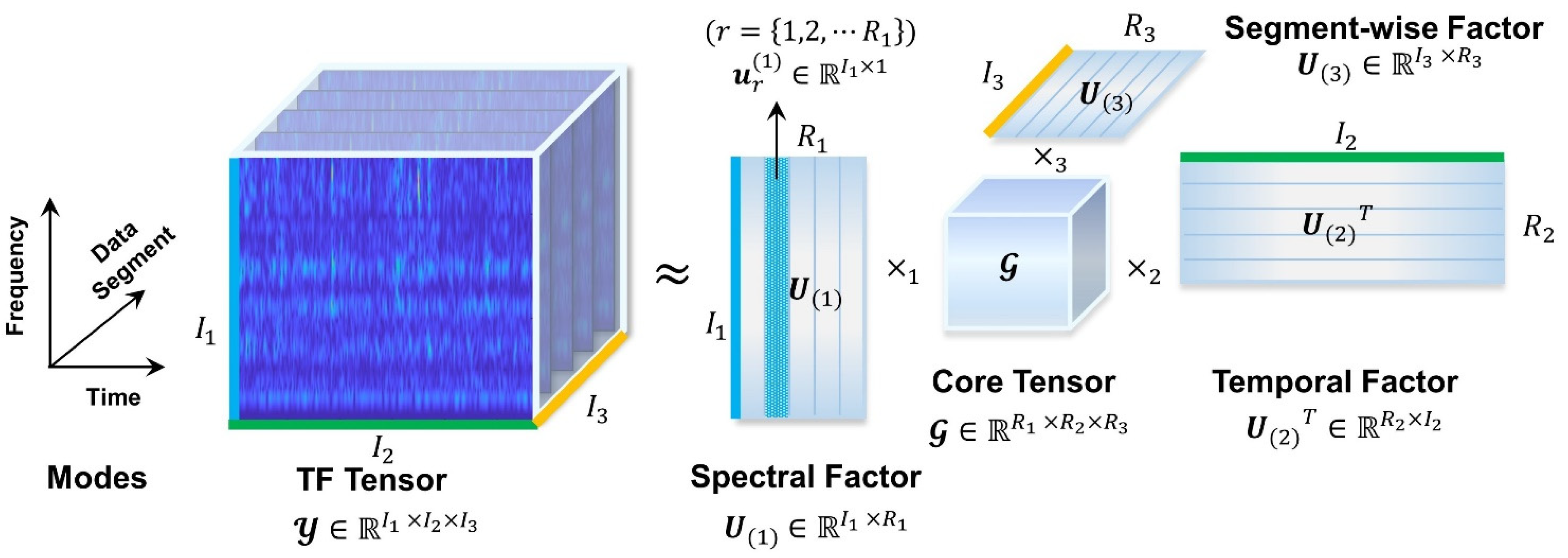
3.2.2. Tensorization: Generating the Time-Frequency Tensor
- Tensors are natural representations for multi-way data beyond the dimensional restriction of matrix analysis, which makes possible the data mining for higher-order connections among multi-channel vibration measurements;
- The time-frequency signatures of localized faults in AFBs are likely to be low-rank, as inherited by the repetitive occurrences of the impact-like structures in the TF spectrogram. It is therefore straight-forward to represent the signature-of-interest through low-rank learning models.
3.2.3. Tensor Decomposition by LRANTD
- (1)
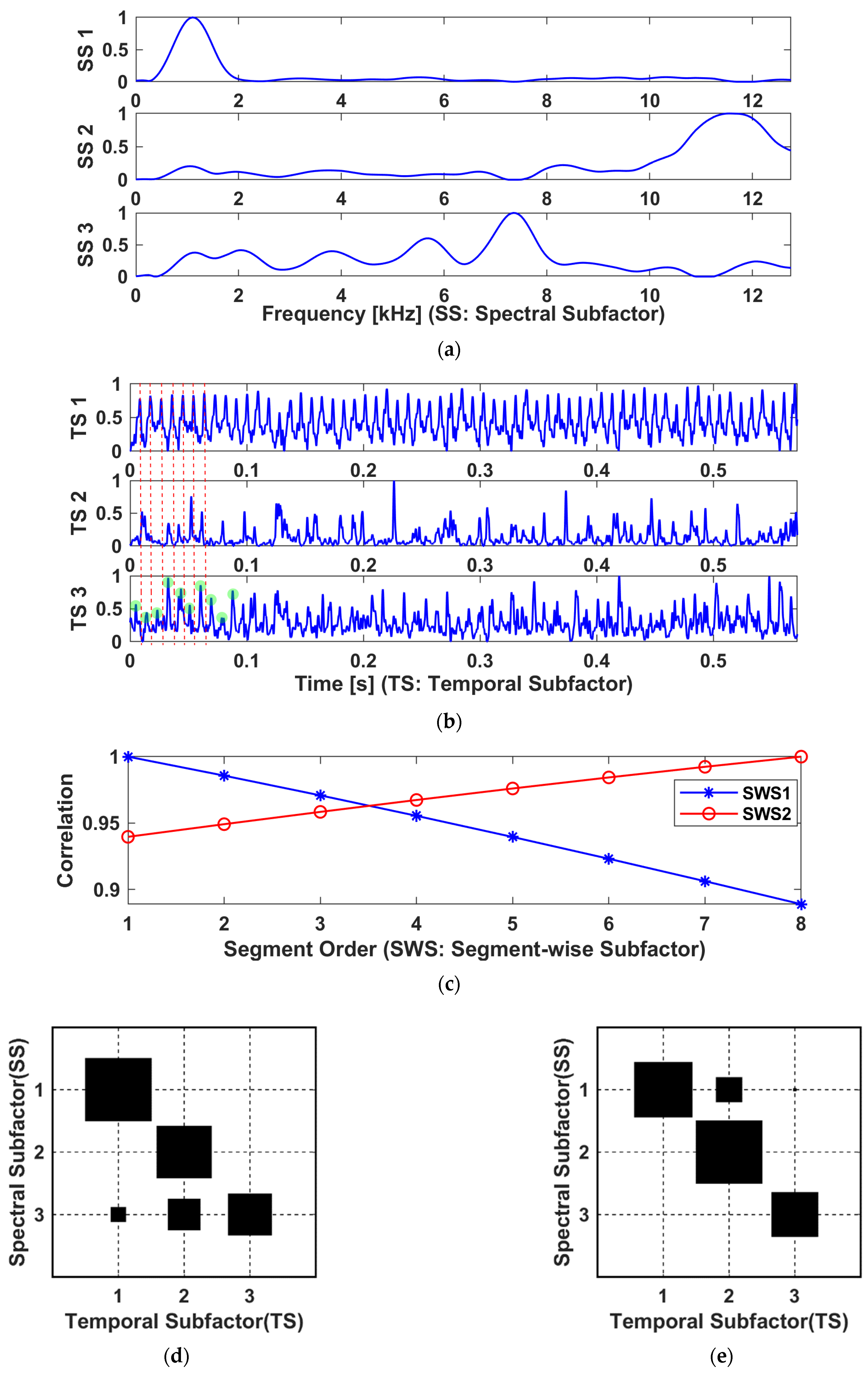
- Based on the proposed method, the latent frequency bands of the TF spectrograms can be automatically extracted without subjective selection. The mode- matrix is called the spectral factor that preserves the dominant frequency bands or spectral subfactors (SS) in its columns, . Each SS is normalized within the interval to indicate the informative bands, which in turn rescales the corresponding temporal pattern to have meaningful amplitude;
- (2)
- The mode- matrix serves as the temporal factor that adaptively identifies the principal encoding patterns or the temporal subfactors (TS) embedded in the corresponding frequency bands. Essentially, these temporal components are the envelope profiles that reveal the variation in TF energy within the informative bands as extracted in the corresponding SS;
- (3)
- Similarly, the mode- matrix clusters data segments into segment-wise subfactors (SWS). Each SWS gives a hint about its relevance to the segments and sensor channels (or spatial locations). For multi-sensor measurements, the multiple SWS represent the dominating spatial components;
- (4)
- Therefore, the entries of the core tensor reflects the correlations across the spectral, the temporal, and the spatial dimensions, which can be visualized intuitively. In other words, the core tensor provides direct information about the spectral locations of the linked temporal patterns.
3.2.4. Evaluation Based on Spectrum Inspection
4. Data Analysis and Case Studies
4.1. Case A
- (1)
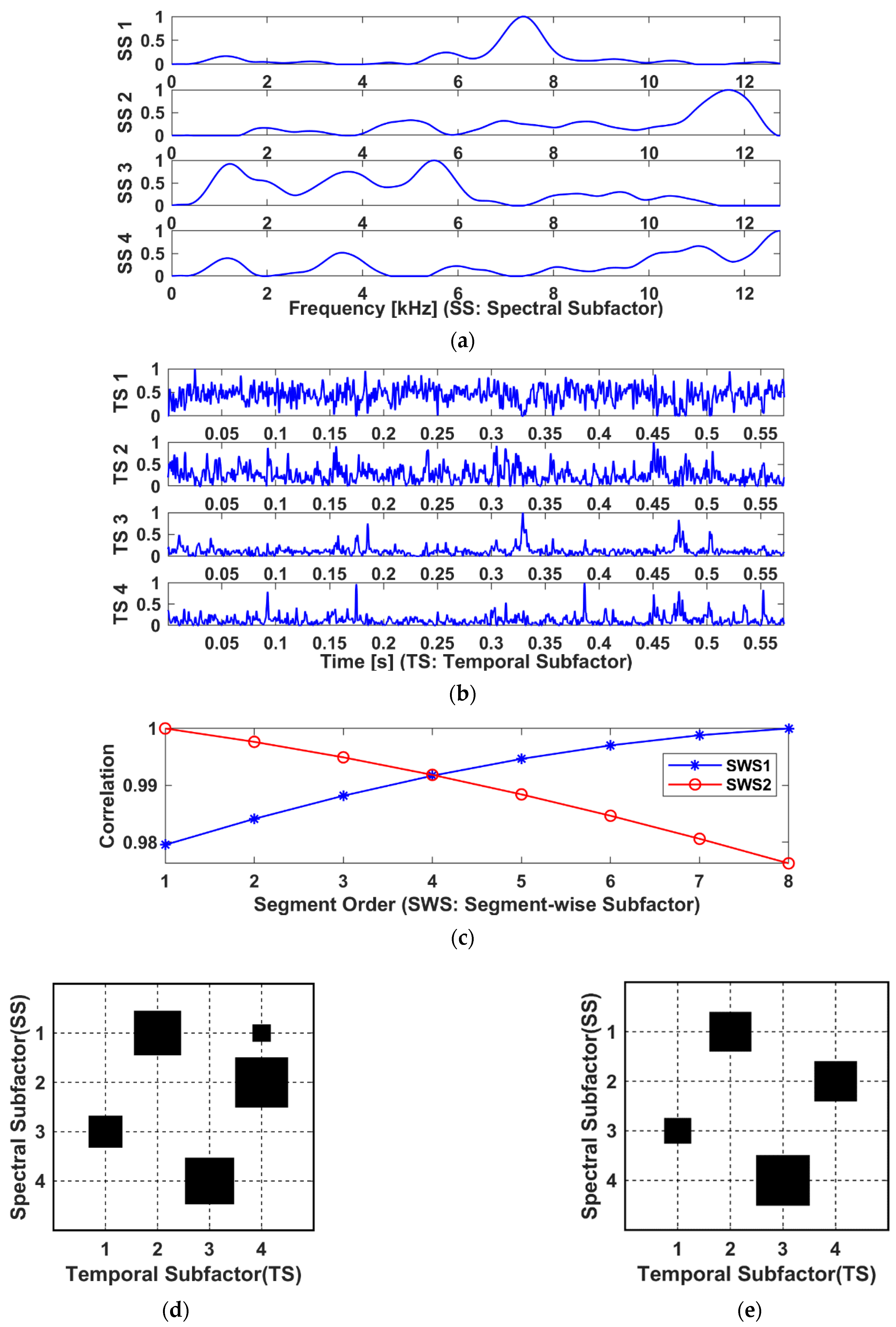
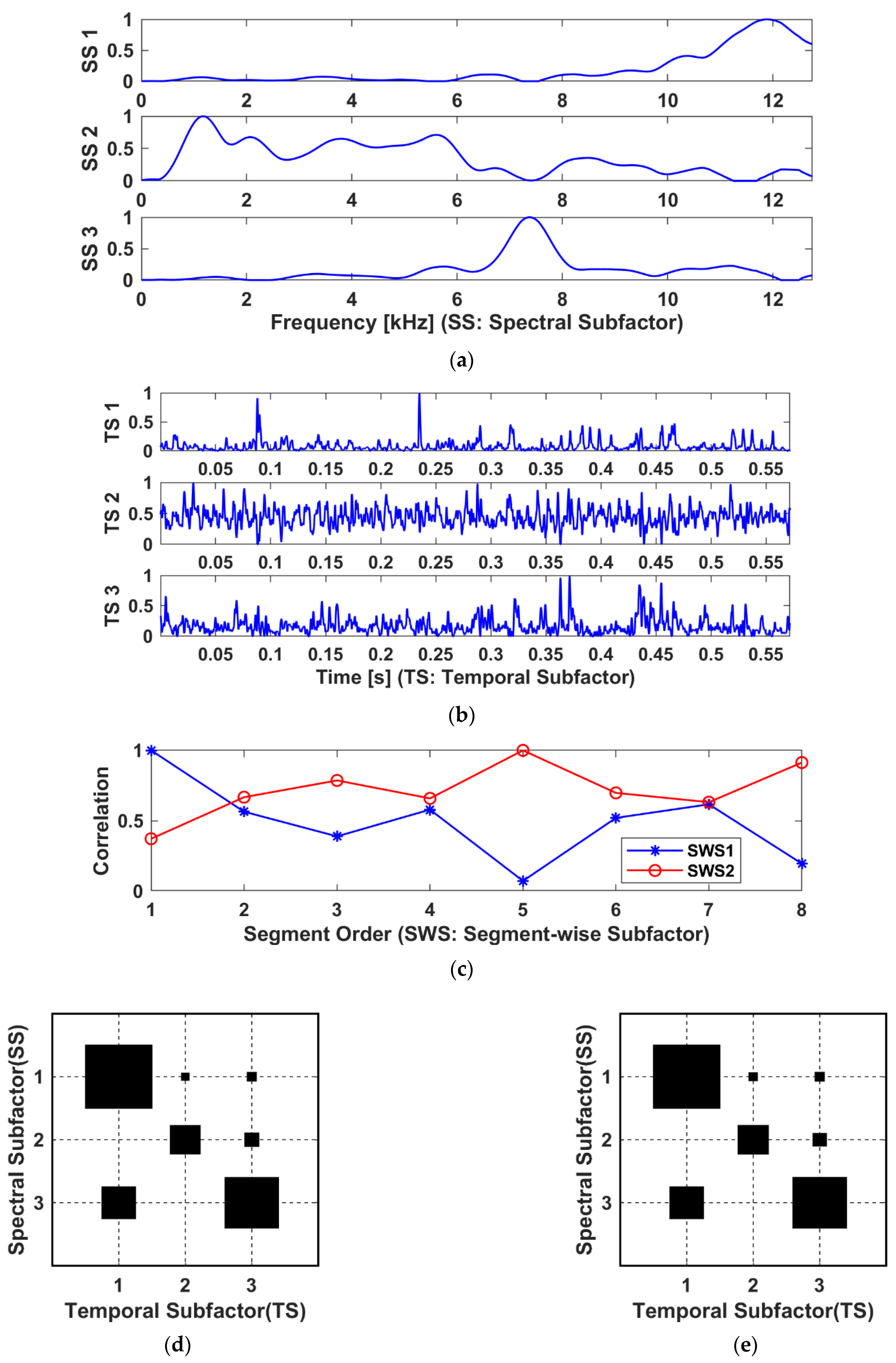
- Note that each SS in had been normalized to intuitively reveal the spectral weight of the correlated TS, thereby adaptively extracted multiple dominant bands from the TF tensor, as shown in Figure 7a;
- (2)
- For the temporal factor , it was found that the TS 3 and TS 4 exhibit apparent impulsive features and have relatively higher kurtosis, as shown in Figure 7b:
- (3)
- Each SWS in the segment-wise factor was found to have a correlation of over 97% to all data segments. This is because all data segments are sampled from the same channel measurement and hence resemble one another;
- (4)
- Unlike the NMF factors, the mode matrices of LRANTD are implicitly linked with one another due to the flexible choice of lower rank dimensions. Such interconnections are embedded in entries of the core tensor, . For visualization, the Hinton diagram of each frontal slice of the core tensor is shown in Figure 7d,e. For example, from Figure 7d, TS 4 was found to have a more distinctive correlation with SS 2 against SS 1, indicating TS 4 is more likely to contain high-frequency components as inferred from Figure 7a.
4.2. Case B
4.3. Case C
5. Comparisons with Benchmark Methods
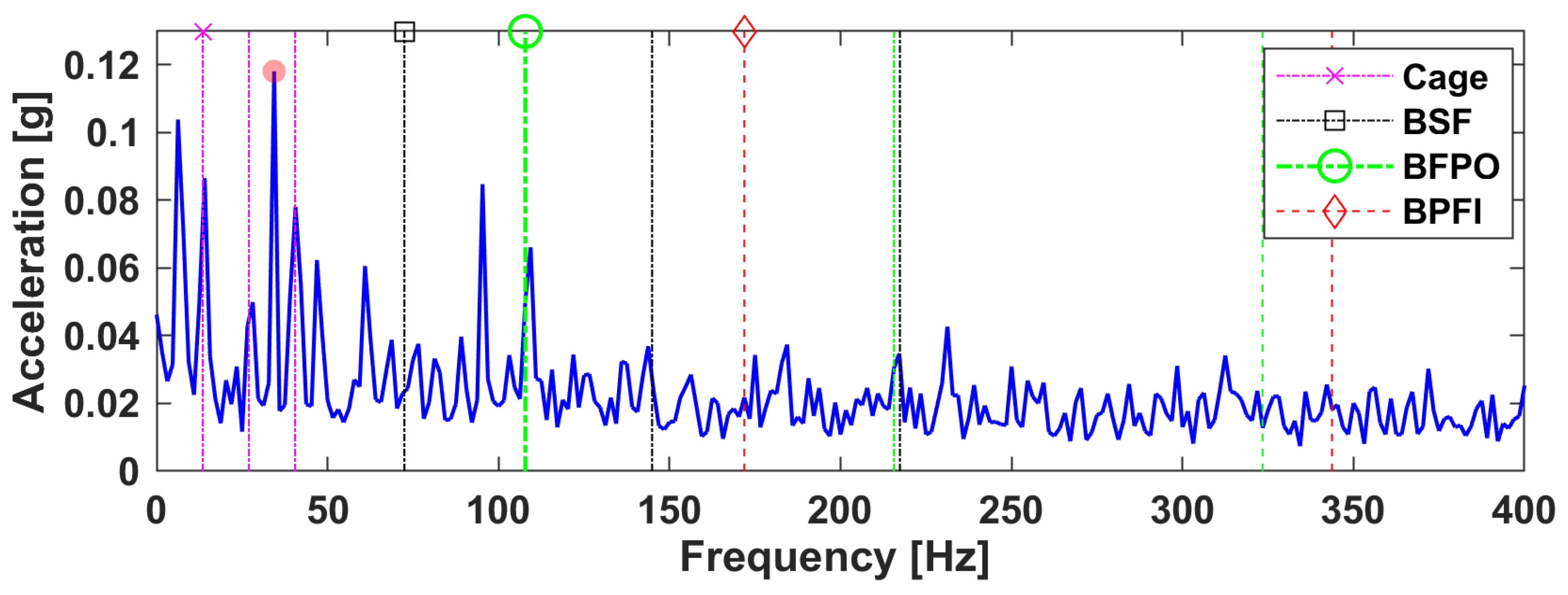
5.1. Envelope Analysis
5.2. Fast Kurtogram
5.3. Empirical Mode Decomposition
6. Cross-Spectrum Methods Based on Sensor Fusion
6.1. The Cross-Spectrum Based on LRANTD
6.2. The Conventional Method
7. Summary of Observations
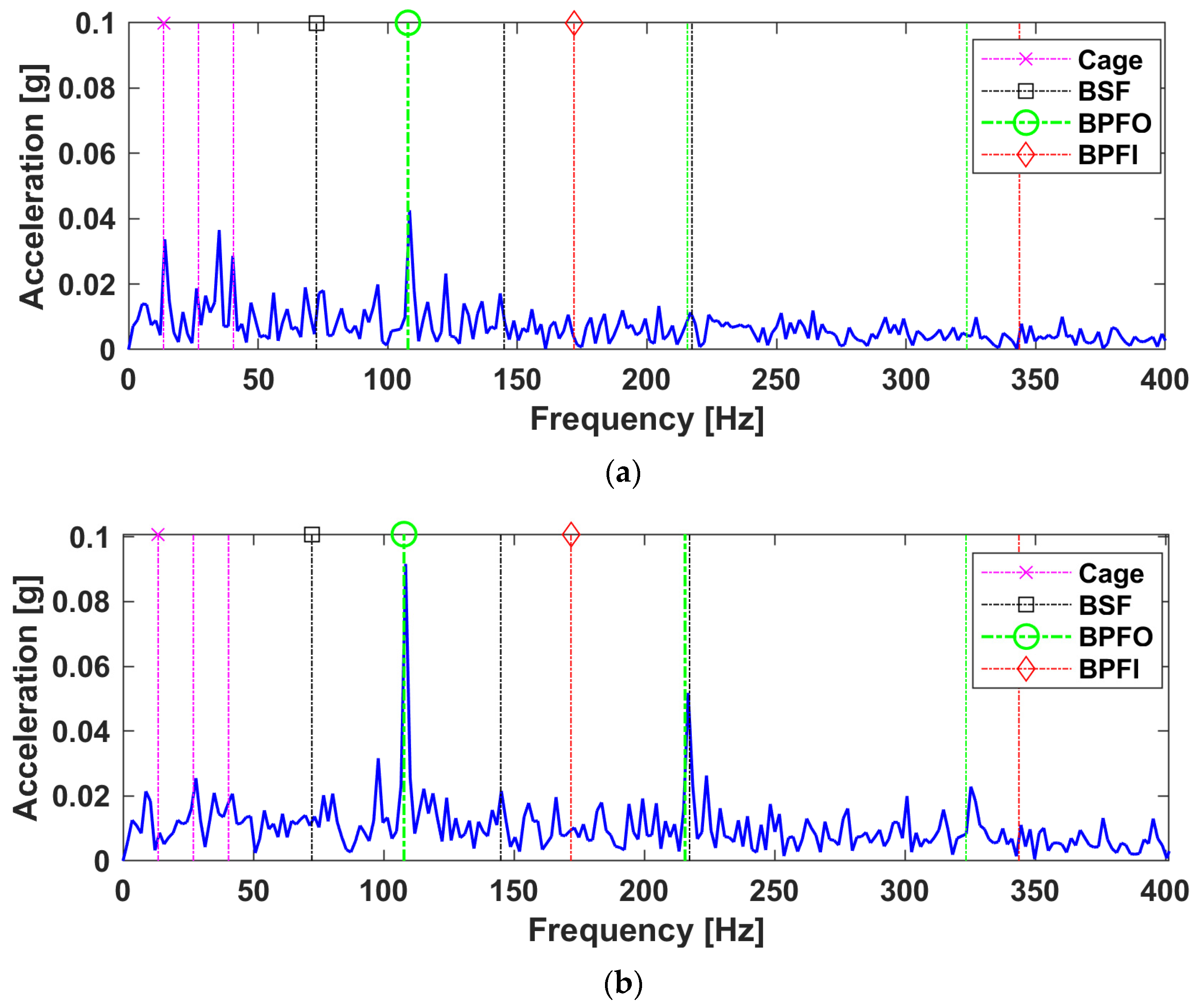
- (i)
- Reducing the presence of the shaft speed related frequency;
- (ii)
- The signal-to-noise ratio is much better for the proposed LRANTD method, hence improving the appearance of the bearing defect frequencies in the spectrum;
- (iii)
- Significant improvements in the BPFO amplitude, generally in the order of 90% for the sensor fusion cases (B and C) compared to the envelope cross-spectrum.
8. Conclusions
Author Contributions
Funding
Institutional Review Board Statement
Informed Consent Statement
Data Availability Statement
Acknowledgments
Conflicts of Interest
References
- Wang, J.; Xu, C.; Zhang, J.; Zhong, R. Big Data Analytics for Intelligent Manufacturing Systems: A Review. J. Manuf. Syst. 2022, 62, 738–752. [Google Scholar] [CrossRef]
- Loutas, T.H.; Roulias, D.; Georgoulas, G. Remaining Useful Life Estimation in Rolling Bearings Utilizing Data-Driven Probabilistic E-Support Vectors Regression. IEEE Trans. Reliab. 2013, 62, 821–832. [Google Scholar] [CrossRef]
- McDonald, G.L.; Zhao, Q. Multipoint Optimal Minimum Entropy Deconvolution and Convolution Fix: Application to Vibration Fault Detection. Mech. Syst. Signal Process. 2017, 82, 461–477. [Google Scholar] [CrossRef]
- Antoni, J. Fast Computation of the Kurtogram for the Detection of Transient Faults. Mech. Syst. Signal Process. 2007, 21, 108–124. [Google Scholar] [CrossRef]
- Antoni, J.; Xin, G.; Hamzaoui, N. Fast Computation of the Spectral Correlation. Mech. Syst. Signal Process. 2017, 92, 248–277. [Google Scholar] [CrossRef]
- Randall, R.B.; Antoni, J.; Gryllias, K. Alternatives to Kurtosis as an Indicator of Rolling Element Bearing Faults. In Proceedings of the ISMA 2016—International Conference on Noise and Vibration Engineering and USD2016—International Conference on Uncertainty in Structural Dynamics, Leuven, Belgium, 19–21 September 2016. [Google Scholar]
- Ding, Y.; He, W.; Chen, B.; Zi, Y.; Selesnick, I.W. Detection of Faults in Rotating Machinery Using Periodic Time-Frequency Sparsity. J. Sound Vib. 2016, 382, 357–378. [Google Scholar] [CrossRef]
- Feng, Z.; Zhou, Y.; Zuo, M.J.; Chu, F.; Chen, X. Atomic Decomposition and Sparse Representation for Complex Signal Analysis in Machinery Fault Diagnosis: A Review with Examples. Measurement 2017, 103, 106–132. [Google Scholar] [CrossRef]
- Chen, Z. Rolling Bearing Fault Diagnosis with Compressed Signals Based on Hybrid Compressive Sensing. J. Vibroeng. 2022, 24, 18–29. [Google Scholar] [CrossRef]
- Yang, B.; Liu, R.; Chen, X. Fault Diagnosis for a Wind Turbine Generator Bearing via Sparse Representation and Shift-Invariant K-SVD. IEEE Trans. Ind. Inform. 2017, 13, 1321–1331. [Google Scholar] [CrossRef]
- Arcos Jiménez, A.; Zhang, L.; Gómez Muñoz, C.Q.; García Márquez, F.P. Maintenance Management Based on Machine Learning and Nonlinear Features in Wind Turbines. Renew. Energy 2020, 146, 316–328. [Google Scholar] [CrossRef]
- Senanayaka, J.S.L.; Van Khang, H.; Robbersmyr, K.G. Toward Self-Supervised Feature Learning for Online Diagnosis of Multiple Faults in Electric Powertrains. IEEE Trans. Ind. Inform. 2021, 17, 3772–3781. [Google Scholar] [CrossRef]
- Sepulveda, N.E.; Sinha, J. Parameter Optimisation in the Vibration-Based Machine Learning Model for Accurate and Reliable Faults Diagnosis in Rotating Machines. Machines 2020, 8, 66. [Google Scholar] [CrossRef]
- Espinoza-Sepulveda, N.; Sinha, J. Mathematical Validation of Experimentally Optimised Parameters Used in a Vibration-Based Machine-Learning Model for Fault Diagnosis in Rotating Machines. Machines 2021, 9, 155. [Google Scholar] [CrossRef]
- Luwei, K.C.; Sinha, J.K.; Yunusa-Kaltungo, A.; Elbhbah, K. Data Fusion of Acceleration and Velocity Features (DFAVF) Approach for Fault Diagnosis in Rotating Machines. MATEC Web Conf. 2018, 211, 21005. [Google Scholar] [CrossRef]
- Wodecki, J.; Kruczek, P.; Bartkowiak, A.; Zimroz, R.; Wyłomańska, A. Novel Method of Informative Frequency Band Selection for Vibration Signal Using Nonnegative Matrix Factorization of Spectrogram Matrix. Mech. Syst. Signal Process. 2019, 130, 585–596. [Google Scholar] [CrossRef]
- Wodecki, J.; Michalak, A.; Zimroz, R.; Wyłomańska, A. Separation of Multiple Local-Damage-Related Components from Vibration Data Using Nonnegative Matrix Factorization and Multichannel Data Fusion. Mech. Syst. Signal Process. 2020, 145, 106954. [Google Scholar] [CrossRef]
- Liang, L.; Ding, X.; Wen, H.; Liu, F. Impulsive Components Separation Using Minimum-Determinant KL-Divergence NMF of Bi-Variable Map for Bearing Diagnosis. Mech. Syst. Signal Process. 2022, 175, 109129. [Google Scholar] [CrossRef]
- Liang, L.; Shan, L.; Liu, F.; Niu, B.; Xu, G. Sparse Envelope Spectra for Feature Extraction of Bearing Faults Based on NMF. Appl. Sci. 2019, 9, 755. [Google Scholar] [CrossRef]
- He, Q.; Ding, X. Time-Frequency Manifold for Machinery Fault Diagnosis. In Smart Sensors, Measurement and Instrumentation; Structural Health Monitoring; Springer: Cham, Switzerland, 2017; Volume 26, pp. 131–154. [Google Scholar]
- Harshman, R. A Foundations of the PARAFAC Procedure: Models and Conditions for an “Explanatory” Multimodal Factor Analysis. UCLA Work. Pap. Phon. 1970, 16, 1–84. [Google Scholar]
- Tucker, L.R. Some Mathematical Notes on Three-Mode Factor Analysis. Psychometrika 1966, 31, 279–311. [Google Scholar] [CrossRef]
- Cichocki, A.; Mandic, D.; De Lathauwer, L.; Zhou, G.; Zhao, Q.; Caiafa, C.; PHAN, H.A. Tensor Decompositions for Signal Processing Applications: From Two-Way to Multiway Component Analysis. IEEE Signal Process. Mag. 2015, 32, 145–163. [Google Scholar] [CrossRef]
- Miron, S.; Zniyed, Y.; Boyer, R.; de Almeida, A.L.F.; Favier, G.; Brie, D.; Comon, P. Tensor Methods for Multisensor Signal Processing. IET Signal Process. 2020, 14, 693–709. [Google Scholar] [CrossRef]
- Zhao, H.; Zhang, W.; Wang, G. Fault Diagnosis Method for Wind Turbine Rolling Bearings Based on Hankel Tensor Decomposition. IET Renew. Power Gener. 2019, 13, 220–226. [Google Scholar] [CrossRef]
- He, Z.; Shao, H.; Cheng, J.; Zhao, X.; Yang, Y. Support Tensor Machine with Dynamic Penalty Factors and Its Application to the Fault Diagnosis of Rotating Machinery with Unbalanced Data. Mech. Syst. Signal Process. 2020, 141, 106441. [Google Scholar] [CrossRef]
- Hu, C.; Wang, Y. Multidimensional Denoising of Rotating Machine Based on Tensor Factorization. Mech. Syst. Signal Process. 2019, 122, 273–289. [Google Scholar] [CrossRef]
- Liang, L.; Wen, H.; Liu, F.; Li, G.; Li, M. Feature Extraction of Impulse Faults for Vibration Signals Based on Sparse Non-Negative Tensor Factorization. Appl. Sci. 2019, 9, 3642. [Google Scholar] [CrossRef]
- Wen, H.; Liang, L.; Niu, B.; Shan, L.; Li, M.; Li, G. The Separation of Vibration Components Based on Sparse Nonnegative Tensor Factorization. In Smart Innovation, Systems and Technologies: Advances in Asset Management and Condition Monitoring; Springer: Berlin/Heidelberg, Germany, 2020; pp. 1297–1306. ISBN 9783030577445. [Google Scholar]
- Zhou, G.; Cichocki, A.; Zhao, Q.; Xie, S. Efficient Nonnegative Tucker Decompositions: Algorithms and Uniqueness. IEEE Trans. Image Process. 2015, 24, 4990–5003. [Google Scholar] [CrossRef]
- Zhou, G.; Cichocki, A.; Xie, S. Fast Nonnegative Matrix/Tensor Factorization Based on Low-Rank Approximation. IEEE Trans. Signal Process. 2012, 60, 2928–2940. [Google Scholar] [CrossRef]
- Wang, B.; Lei, Y.; Li, N.; Li, N. A Hybrid Prognostics Approach for Estimating Remaining Useful Life of Rolling Element Bearings. IEEE Trans. Reliab. 2018, 69, 401–412. [Google Scholar] [CrossRef]
- Kim, Y.D.; Choi, S. Nonnegative Tucker Decomposition. In Proceedings of the IEEE Computer Society Conference on Computer Vision and Pattern Recognition 2007, Minneapolis, MN, USA, 17–22 June 2007. [Google Scholar]
- Lee, D.D.; Seung, H.S. Algorithms for Non-Negative Matrix Factorization. Adv. Neural Inf. Process. Syst. 2001, 13, 556–562. [Google Scholar]
- Phan, A.H.; Cichocki, A. Extended HALS Algorithm for Nonnegative Tucker Decomposition and Its Applications for Multiway Analysis and Classification. Neurocomputing 2011, 74, 1956–1979. [Google Scholar] [CrossRef]
- Cichocki, A.; Zdunek, R.; Amari, S.I. Hierarchical ALS Algorithms for Nonnegative Matrix and 3D Tensor Factorization. In Proceedings of the 7th International Conference, ICA 2007, London, UK, 9–12 September 2007; Volume 4666, pp. 169–176. [Google Scholar] [CrossRef]
- Kim, H.; Park, H. Nonnegative Matrix Factorization Based on Alternating Nonnegativity Constrained Least Squares and Active Set Method. SIAM J. Matrix Anal. Appl. 2008, 30, 713–730. [Google Scholar] [CrossRef]
- Antoni, J.; Randall, R.B. Differential Diagnosis of Gear and Bearing Faults. J. Vib. Acoust. Trans. ASME 2002, 124, 165–171. [Google Scholar] [CrossRef]


| 0 | The vector/matrix with all its entries being zero. |
| , | Nonnegative matrix and its -th column vector. |
| , | Mode- matrix and its -th column vector, . |
| N-way arrays or tensor and its mode- matricizaton. | |
| , | Core tensor and its mode- matricizaton. |
| Low-rank dimensions for NTD, | |
| The index set of positive integers, . | |
| Mode- product, | |
| Kronecker product of and yields | |
| Element-wise multiplication, division | |
| is equal to . If , then . | |
| , | The -th channel acceleration with points in length, within sensors measurement. |
| , | The -th segment resampled from the -th channel signal, the -th entry of . |
| , | Spectrogram matrix with frequency bins and time points, -entry of |
| , | The number of data segments resampled from one signal, the length of each segmentation, the total number of segments |
| Parameter | Value | Characteristics | Value |
|---|---|---|---|
| Mean diameter | 34.55 mm | 35 Hz | |
| Ball diameter | 7.92 mm | 13.49 Hz | |
| Number of balls | 8 | 72.33 Hz | |
| Contact angle | 0° | 107.91 Hz | |
| Load rating | 12 kN | 172.09 Hz |
| Case A (Single-Channel) | Case A (Sensor-Fusion) | |||||
|---|---|---|---|---|---|---|
| Component | Envelope Spectrum | Fast Kurtogram | EMD | LRANTD | (Envelope) CPSD | LRANTD |
| Shaft Speed fr | 0.1115 (5.21) | 0.0138 (6.27) | 0.1181 (5.15) | 0.0211 (2.63) | 0.043 (5.58) | 0.0214 (2.05) |
| Cage Freq. fc | 0.0819 (3.82) | 0.0109 (4.95) | 0.0866 (3.78) | 0.0292 (3.65) | 0.0362 (4.70) | 0.0416 (4.00) |
| BSF fb | 0.0202 (0.94) | 0.0019 (0.86) | 0.0244 (1.06)) | 0.0090 (1.12) | 0.0103 (1.33) | 0.0069 (0.66) |
| BPFOfo | 0.0656 (3.06) | 0.0096 (4.36) | 0.0661 (2.88) | 0.0375 (4.68) | 0.0332 (4.31) | 0.0597 (5.74) * |
| BPFO 2x | 0.0388 (1.81) | 0.0047 (2.13) | 0.0348 (1.51) | 0.0211 (2.63) | 0.0226 (2.93) | 0.0294 (2.82) * |
| BPFO 3x | 0.0230 (1.07) | 0.0021 (0.95) | 0.018 (0.78) | 0.0060 (0.75) | 0.0080 (1.03) | 0.0118 (1.13) * |
| BPFI fi | 0.0209 (0.97) | 0.0043 (1.95) | 0.0218 (0.95) | 0.0123 (1.53) | 0.0117 (1.51) | 0.0115 (1.10) |
| Background Noise | 0.0214 | 0.0022 | 0.0229 | 0.008 | 0.0077 | 0.0104 |
| Remark | BPFO Baseline | +1.30 (+42.48%) | −0.18 (−5.88%) | +1.62 (+52.94%) | BPFO Baseline | +1.43 (+33.18%) |
| Case B (Sensor-Fusion) | Case C (Sensor-Fusion) | |||
|---|---|---|---|---|
| Component | CPSD | LRANTD | CPSD | LRANTD |
| Shaft Speed fr | 0.1244 (7.36) | 0.0217 (2.08) | 0.0958 (6.02) | 0.0394 (4.37) |
| Cage Freq. fc | 0.112 (6.62) | 0.0205 (1.97) | 0.0562 (3.53) | 0.0157 (1.74) |
| BSF fb | 0.0405 (2.39) | 0.0184 (1.76) | 0.0404 (2.54) | 0.0137 (1.52) |
| BPFOfo | 0.0969 (5.73) | 0.1134 (10.90) * | 0.2335 (14.68) | 0.2525 (28.05) * |
| BPFO 2x | 0.0451 (2.66) | 0.0488 (4.69) * | 0.1021 (6.42) * | 0.0464 (5.15) |
| BPFO 3x | 0.0170 (1.01) | 0.0232 (2.23) * | 0.0690 (4.33) | 0.0405 (4.50) * |
| BPFI fi | 0.0128 (0.75) | 0.0146 (1.40) | 0.0126 (0.79) | 0.0054 (0.60) |
| Background Noise | 0.0169 | 0.0104 | 0.0159 | 0.009 |
| Remark | BPFO Baseline | +5.17 (+90.23%) | BPFO Baseline | +13.37 (+91.07%) |
Publisher’s Note: MDPI stays neutral with regard to jurisdictional claims in published maps and institutional affiliations. |
© 2022 by the authors. Licensee MDPI, Basel, Switzerland. This article is an open access article distributed under the terms and conditions of the Creative Commons Attribution (CC BY) license (https://creativecommons.org/licenses/by/4.0/).
Share and Cite
Wen, H.; Zhang, L.; Sinha, J.K. Adaptive Band Extraction Based on Low Rank Approximated Nonnegative Tucker Decomposition for Anti-Friction Bearing Faults Diagnosis Using Measured Vibration Data. Machines 2022, 10, 694. https://doi.org/10.3390/machines10080694
Wen H, Zhang L, Sinha JK. Adaptive Band Extraction Based on Low Rank Approximated Nonnegative Tucker Decomposition for Anti-Friction Bearing Faults Diagnosis Using Measured Vibration Data. Machines. 2022; 10(8):694. https://doi.org/10.3390/machines10080694
Chicago/Turabian StyleWen, Haobin, Long Zhang, and Jyoti K. Sinha. 2022. "Adaptive Band Extraction Based on Low Rank Approximated Nonnegative Tucker Decomposition for Anti-Friction Bearing Faults Diagnosis Using Measured Vibration Data" Machines 10, no. 8: 694. https://doi.org/10.3390/machines10080694