
Application of the Gray Wolf Optimization Algorithm in Active Disturbance Rejection Control Parameter Tuning of an Electro-Hydraulic Servo Unit


Abstract
:1. Introduction
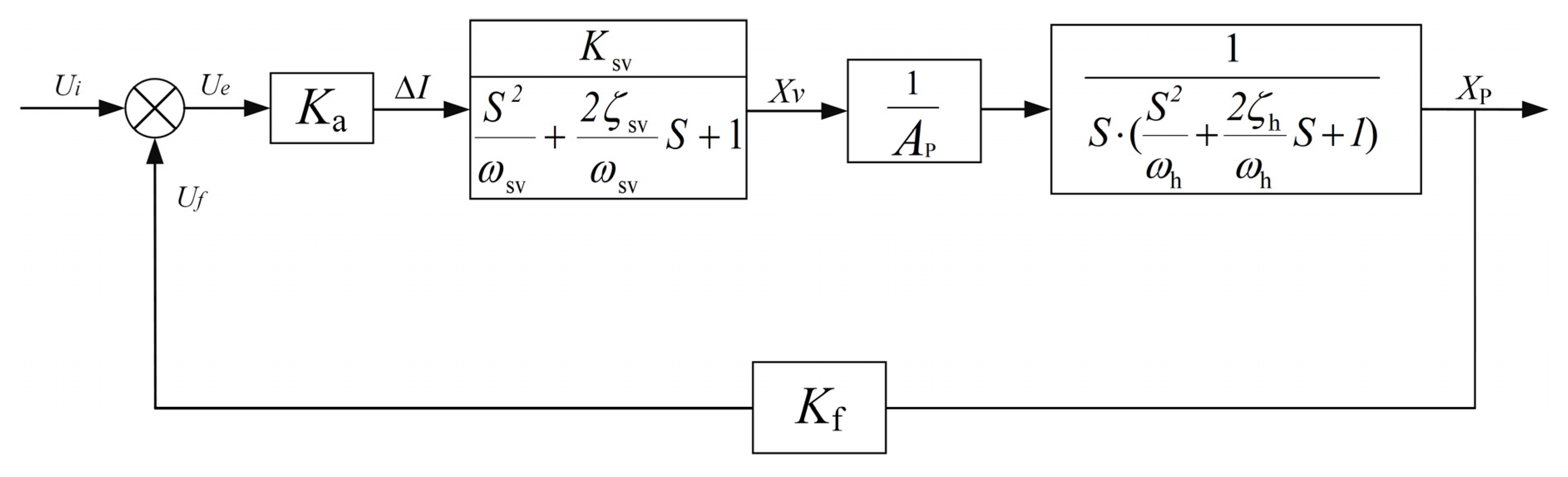
2. Modeling of an Electro-Hydraulic Servo System
3. Design of Auto-Disturbance Rejection Controller Based on Grey Wolf Algorithm
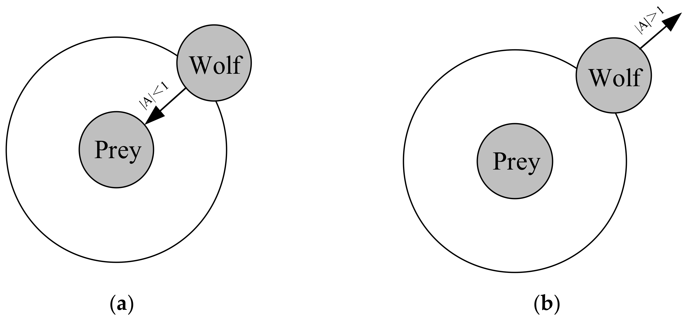
3.1. Grey Wolf Optimization Algorithm
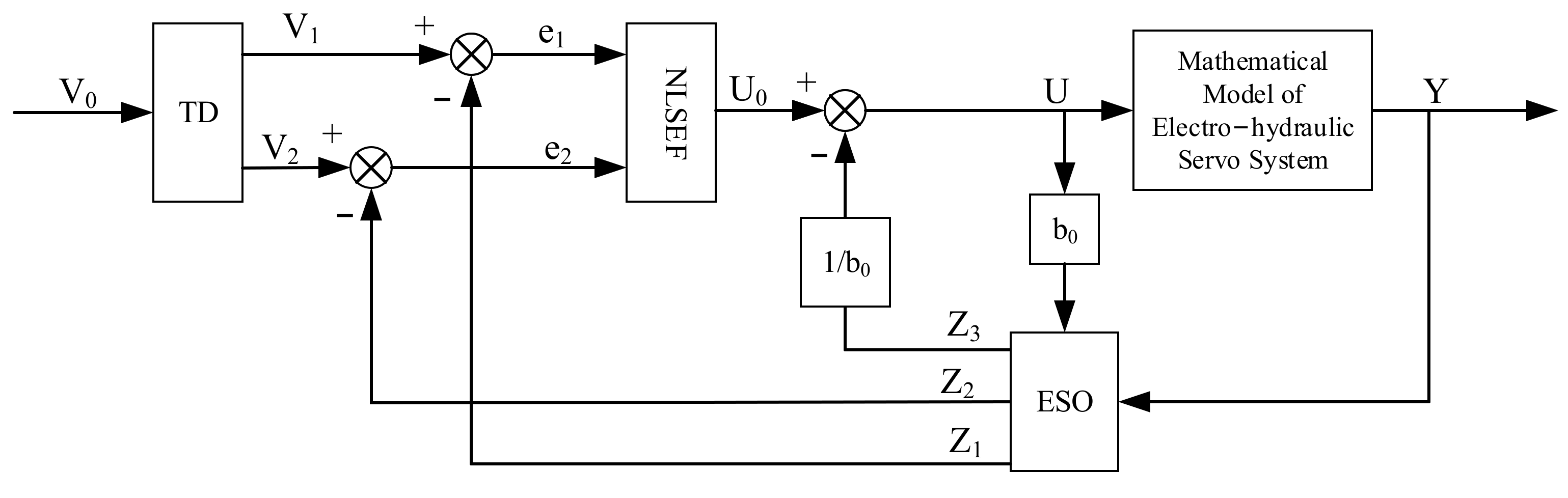
3.2. Design of the Active Disturbance Rejection Controller
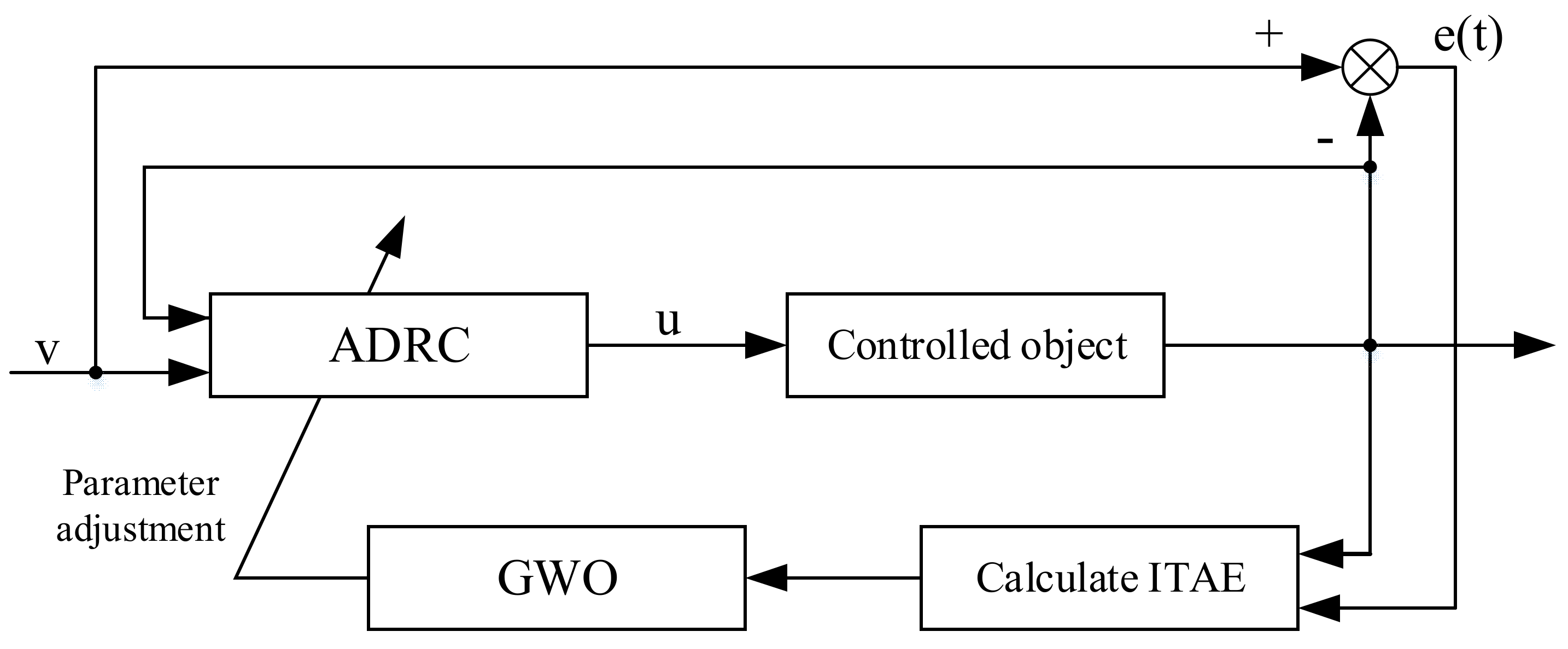
3.3. Parameter Tuning Algorithm Design Based on the Gray Wolf Optimization
3.3.1. Fitness Function
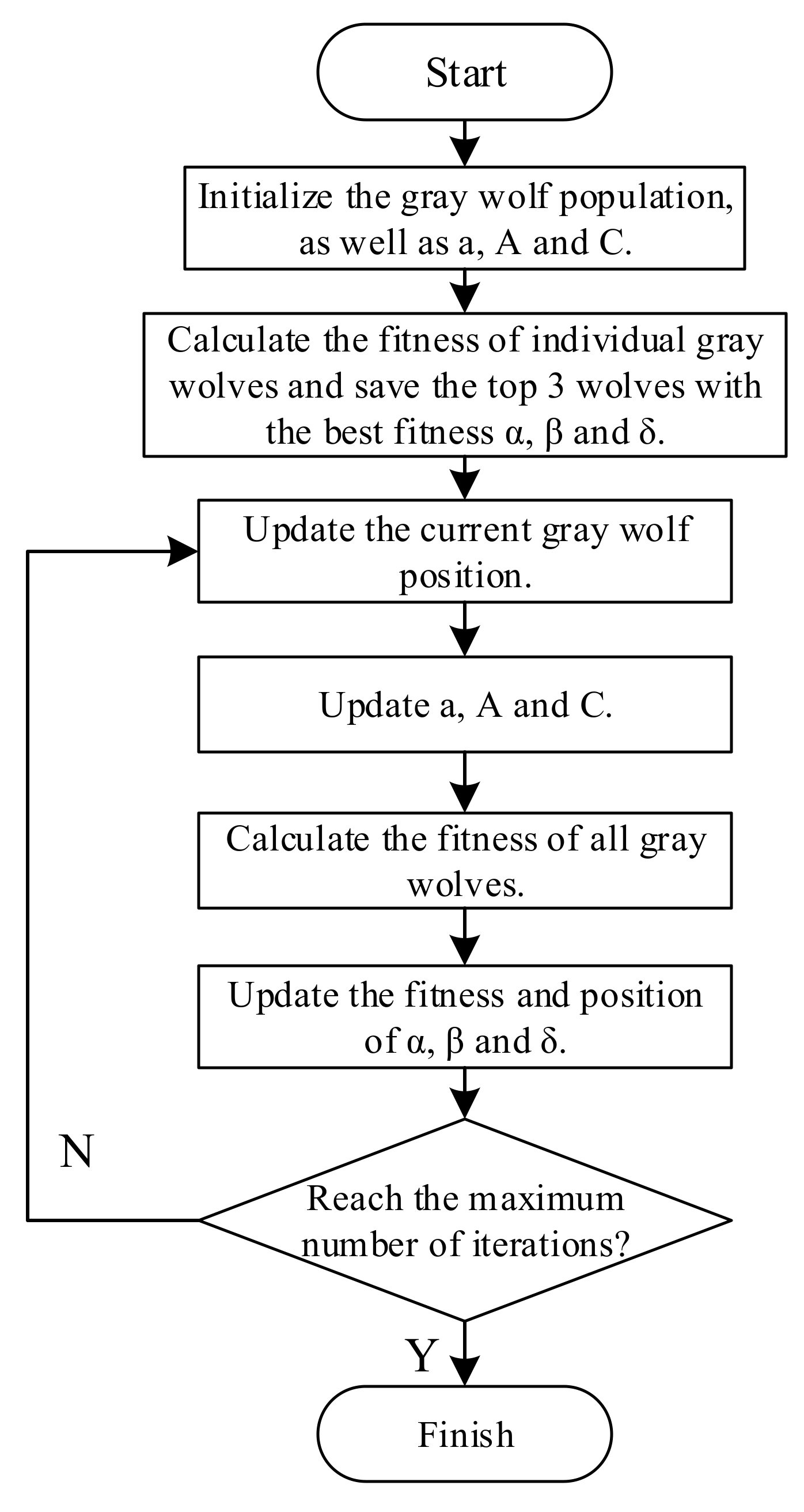
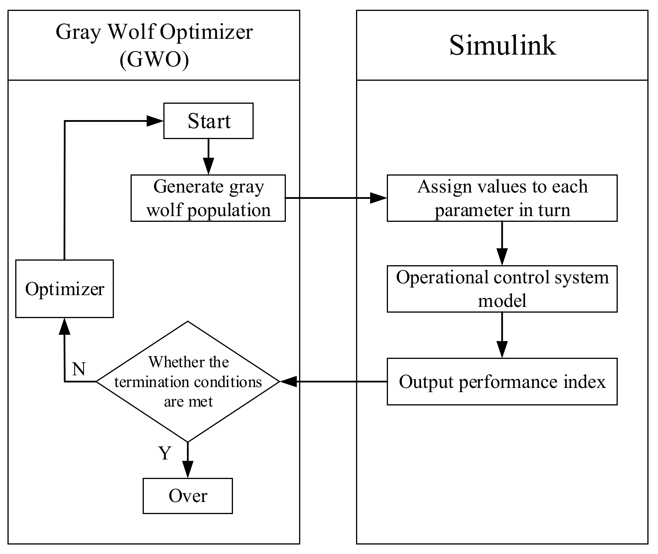
3.3.2. Algorithm Implementation
- Initialize the parameters of the GWO algorithm. Set the population size to 16, the dimension to 5, the maximum number of iterations to 15, and give the value range of each parameter based on the experience value.
- Initialize the location information of the GWO algorithm. Randomly initialize the position information of the artificial gray wolf optimization algorithm (16 parameters of the auto-disturbance rejection controller to be tuned), and use random initialization for the 16 parameters of the auto-disturbance rejection controller, such as, within the range of values. The mechanism initializes the gray wolf position information in the algorithm. Expressed as: . Among them, i is the i-th gray wolf in the population, and corresponds to an auto-disturbance rejection controller parameter to be tuned.
- The Simulink (and AMEsim) program runs. Assign the value to the Simulink module, run the control system model, calculate the corresponding fitness function value, and find the global optimal position in the initialization phase.
- Iterate the algorithm until the termination condition is met. The population is iterated according to Formula (14) to Formula (20), to select the optimal fitness value and its corresponding location information.
- Whether the stop condition is met: generally, a fixed number of iterations or a fitness function value reaching a certain accuracy is selected as the stopping condition of the algorithm.
- Output the position information corresponding to the optimal fitness value and the change of the fitness value during the iteration process. This positional information is the parameter value of of the active disturbance rejection controller. The change curve of the optimal fitness value is the convergence curve of the GWO algorithm.
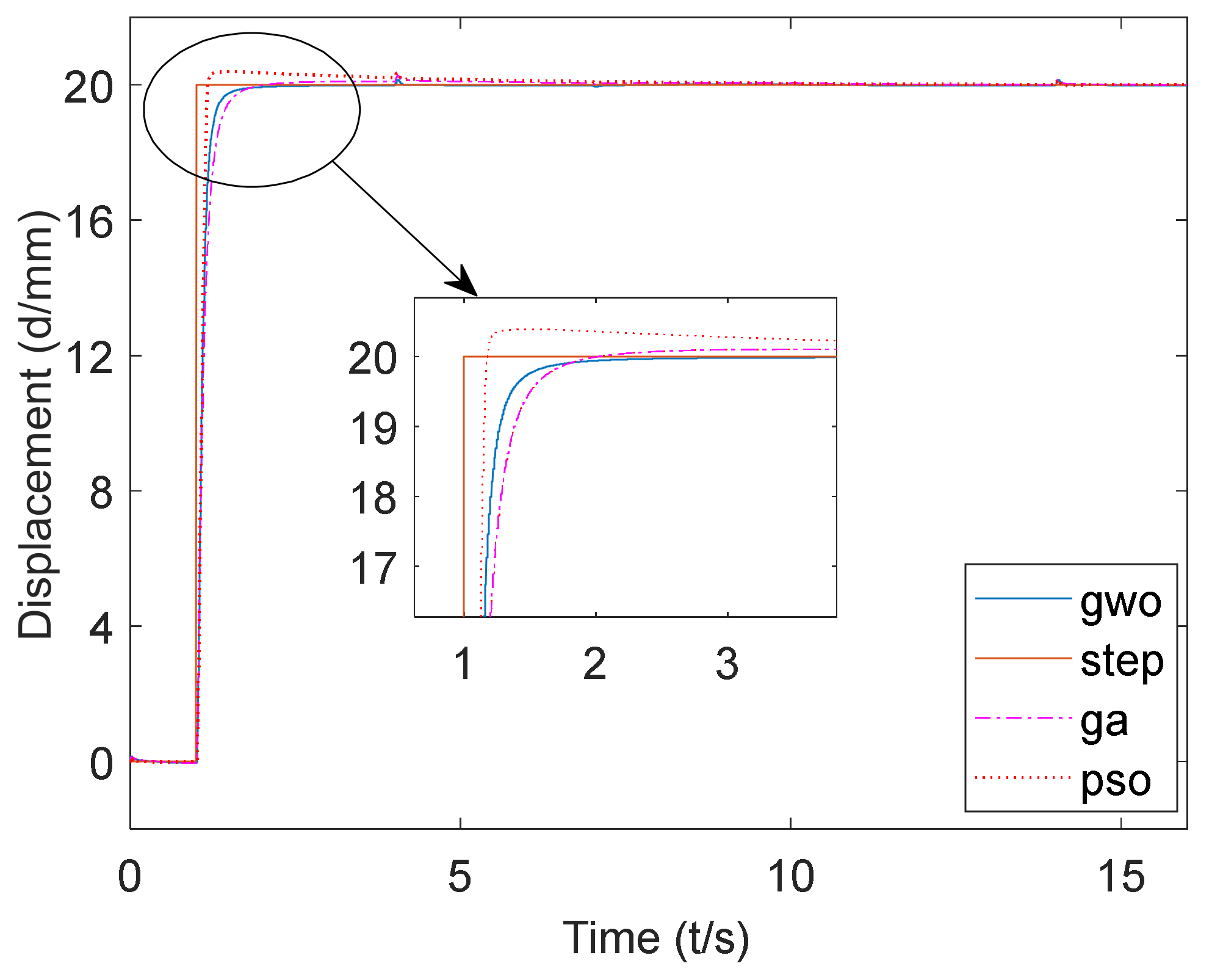
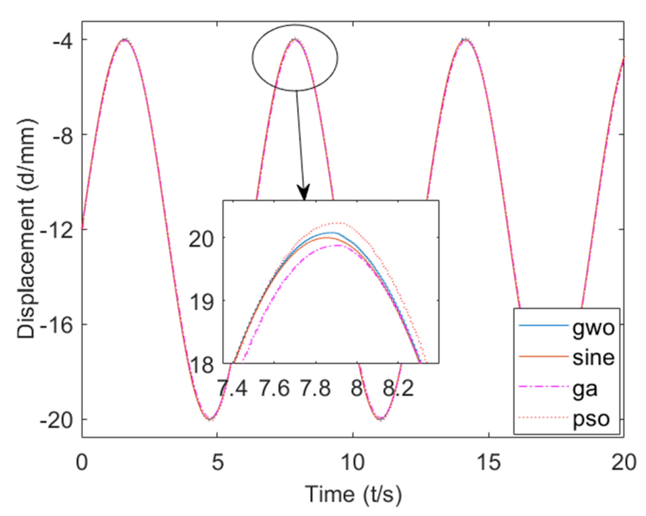
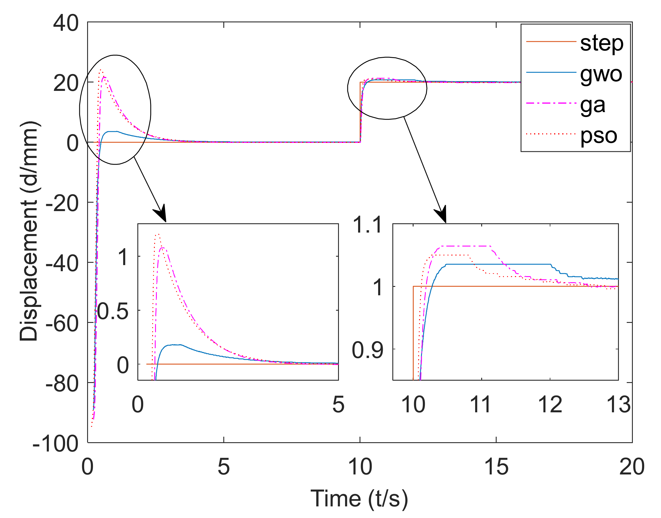
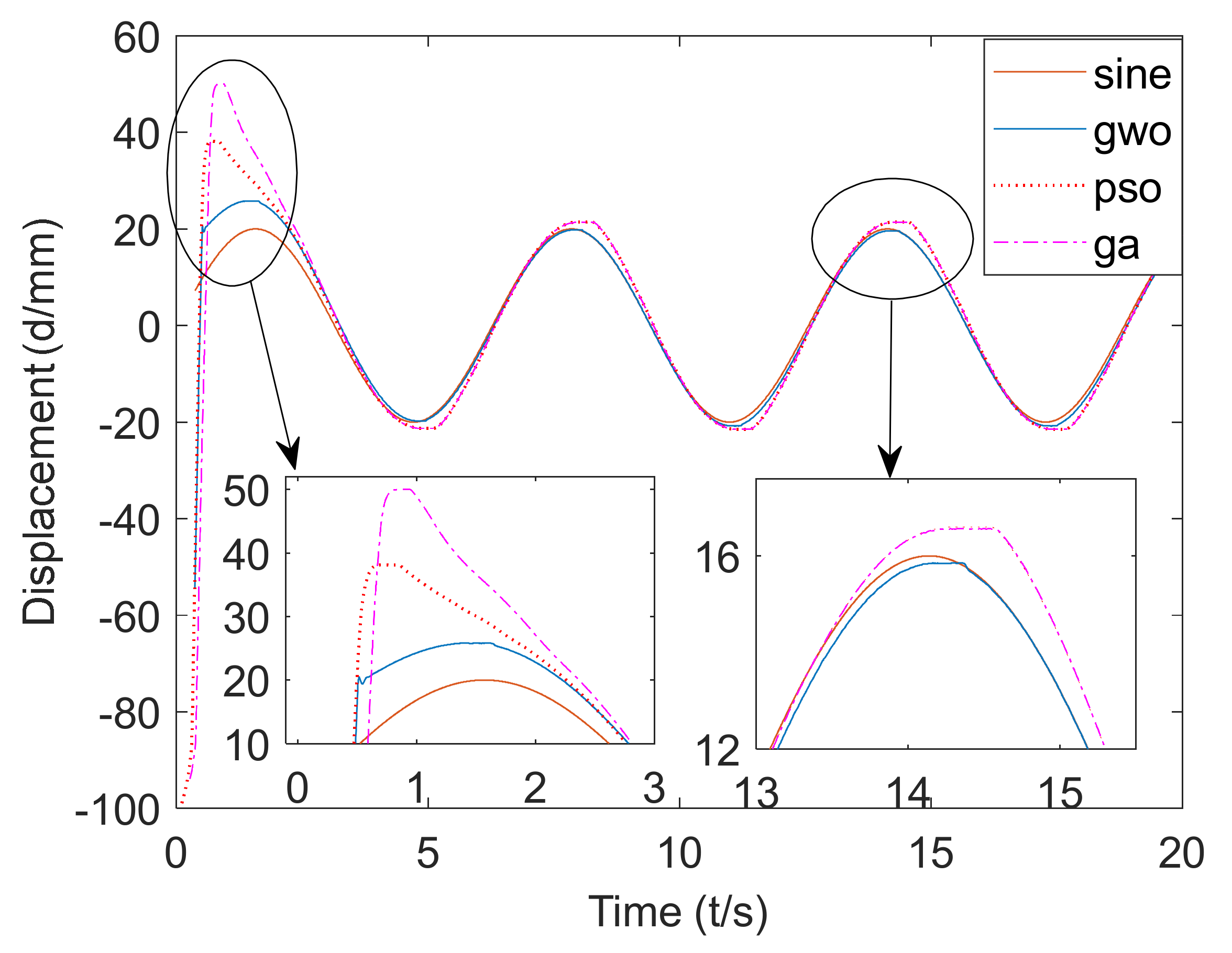
4. Simulation Analysis
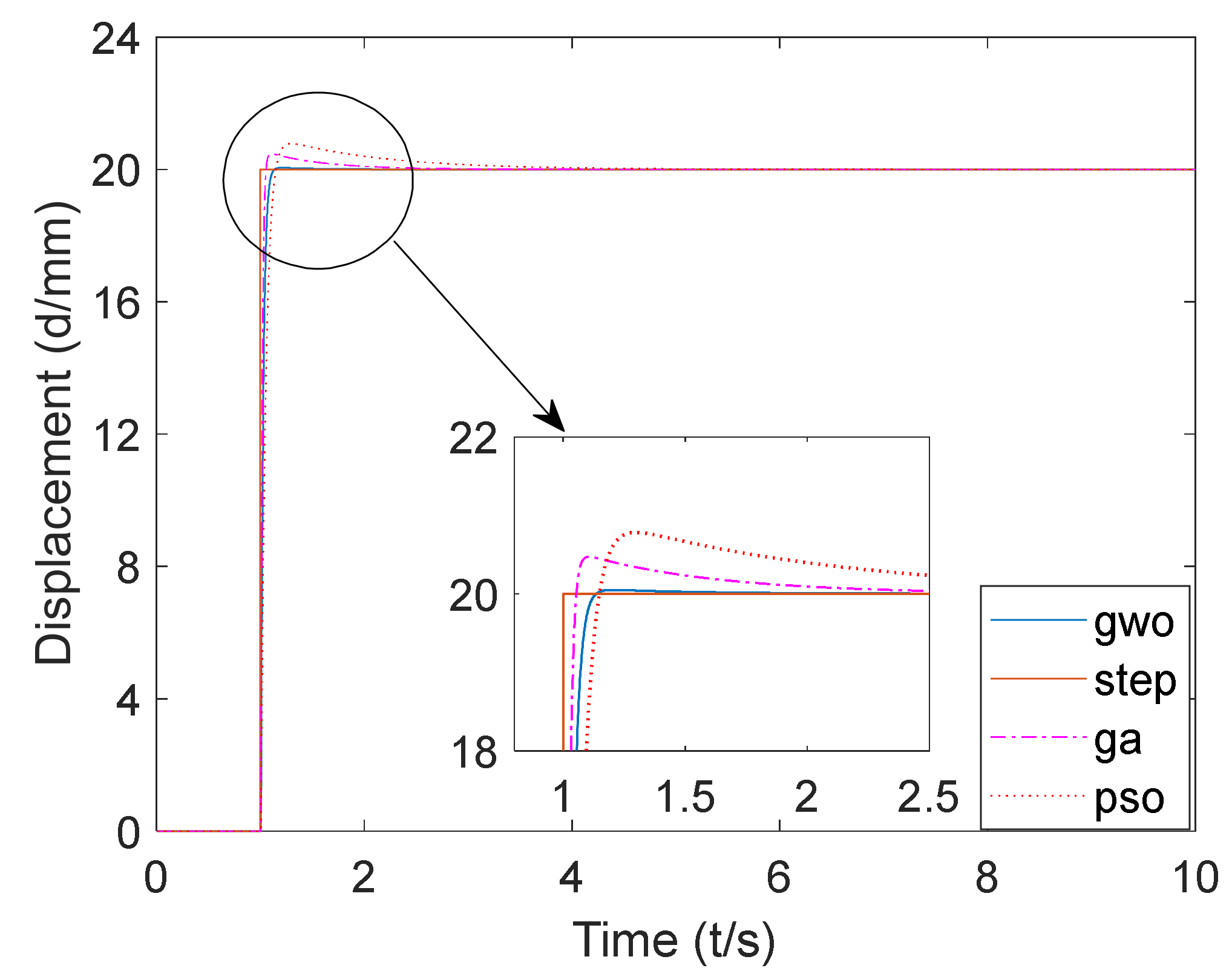
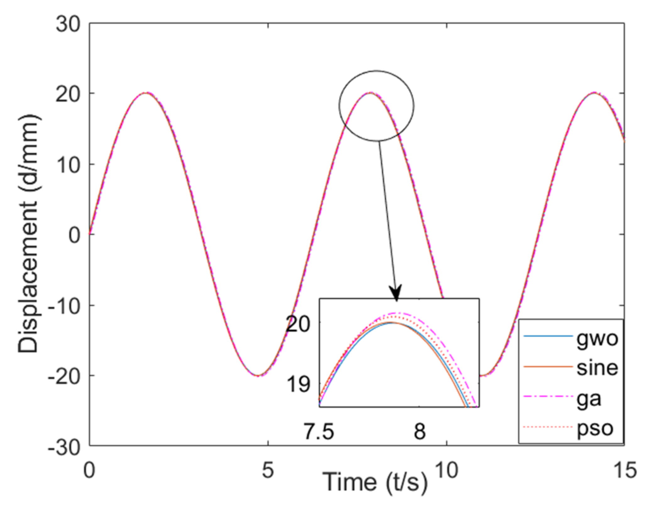
4.1. Simulink Simulation
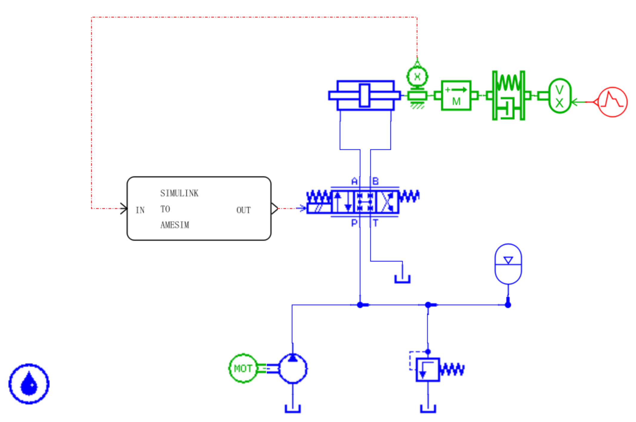
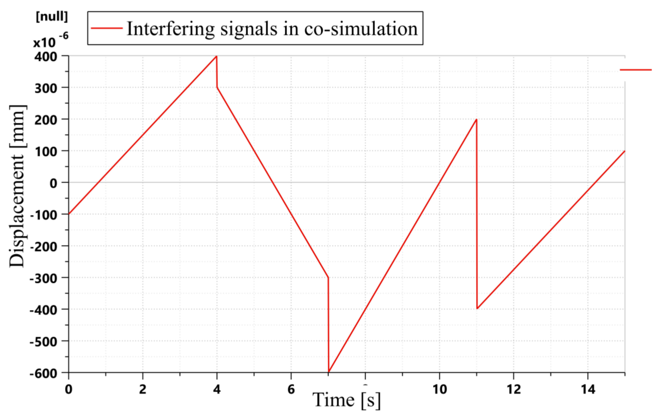
4.2. AMEsim and Simulink Co-Simulation
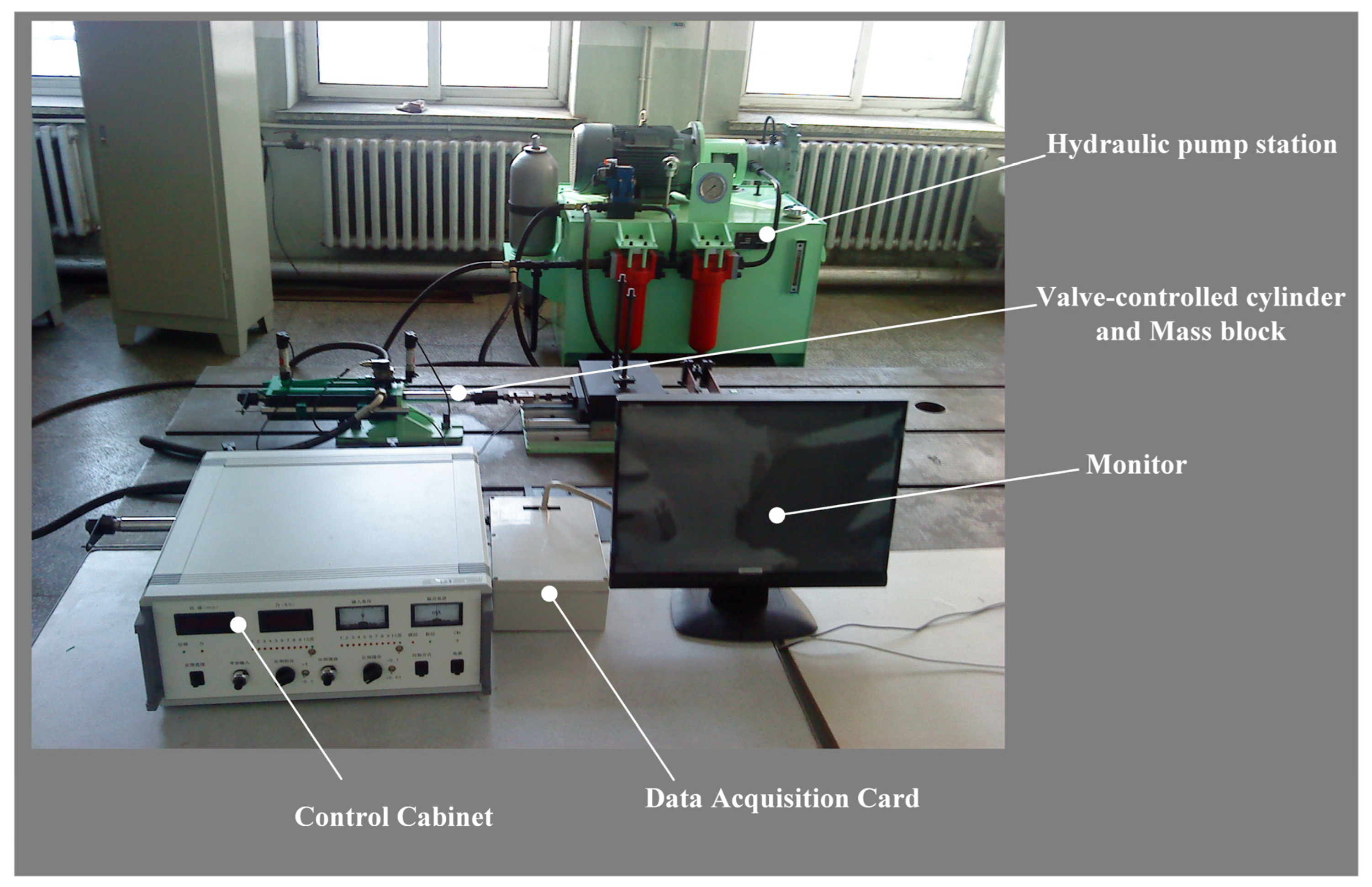
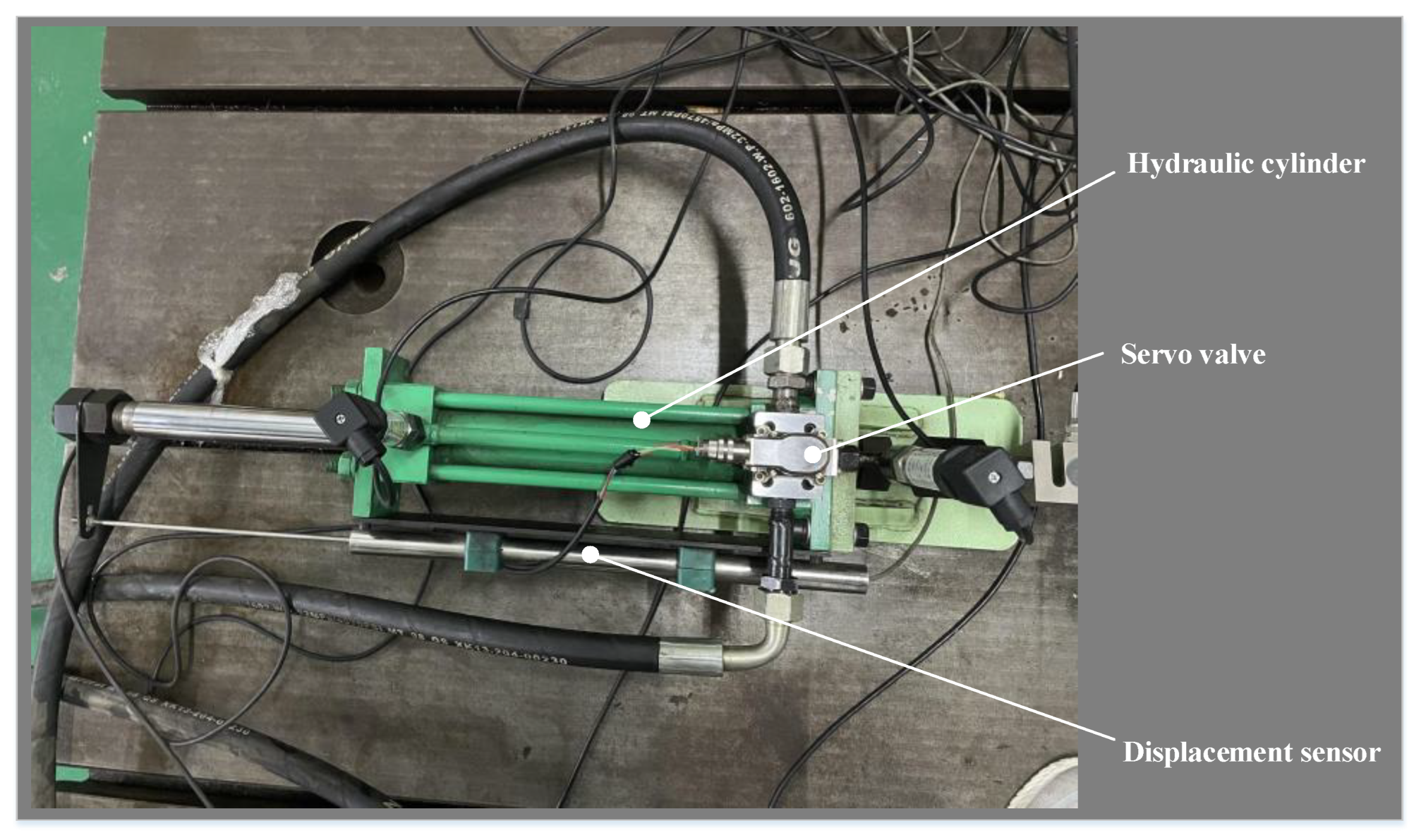
5. Experimental Verification
6. Discussion
7. Conclusions
Author Contributions
Funding
Institutional Review Board Statement
Informed Consent Statement
Data Availability Statement
Conflicts of Interest
References
- Gao, B.; Shen, W.; Guan, H.; Zheng, L.; Zhang, W. Research on Multi-Strategy Improved Evolutionary Sparrow Search Algorithm and its Application. IEEE Access 2022, 10, 62520–62534. [Google Scholar] [CrossRef]
- Wenjie, S.; Honghua, T.; Ming, H.; Jing, Y. Electro-hydraulic Position Servo Control System. Chin. Hydraul. Pneum. 2019, 6, 116–121. [Google Scholar]
- Xuchao, Z. Fault diagnosis of hydraulic servo control system for construction machinery. Wirel. Int. Tech. 2018, 15, 125–126. [Google Scholar]
- Rodríguez-Abreo, O.; Velásquez, F.A.C.; de Paz, J.P.Z.; Godoy, J.L.M.; Guendulain, C.G. Sensorless Estimation Based on Neural Networks Trained with the Dynamic Response Points. Sensors 2021, 21, 6719. [Google Scholar] [CrossRef] [PubMed]
- Rodríguez-Abreo, O.; Garcia-Guendulain, J.M.; Hernández-Alvarado, R.; Rangel, A.F.; Fuentes-Silva, C. Genetic Algorithm-Based Tuning of Backstepping Controller for a Quadrotor-Type Unmanned Aerial Vehicle. Electronics 2020, 9, 1735. [Google Scholar] [CrossRef]
- Junpeng, S.; Lihua, C.; Zhibin, S. The application of fuzzy control strategy in electro-hydraulic servo system. IEEE Int. Conf. Mechatron. Autom. 2005, 4, 2010–2016. [Google Scholar]
- Gao, B.; Shen, W.; Dai, Y.; Ye, Y.T. Parameter tuning of auto disturbance rejection controller based on improved glowworm swarm optimization algorithm. Assem. Autom. 2022, 42, 427–444. [Google Scholar] [CrossRef]
- Wang, L.; Yan, J.; Cao, T.; Liu, N. Manipulator Control Law Design Based on Backstepping and ADRC Methods. In Proceedings of the 2020 Chinese Intelligent Systems Conference, Shenzhen, China, 24–25 October 2021. [Google Scholar]
- Chu, Z.; Jave, H.; Li, D.; Qi, K. Design of an Active Disturbance Rejection Control for Drag-Free Satellite. Microgravity Sci. Technol. 2019, 31, 31–48. [Google Scholar]
- Mehrnoosh, K.; Mohammad, H.R. Intelligent Sliding Mode Adaptive Controller Design for Wind Turbine Pitch Control System Using PSO-SVM in Presence of Disturbance. J. Control Autom. Electr. Syst. 2020, 31, 912–925. [Google Scholar]
- Mehran, R.; Hossein, K.; Mohammad, R. New Sliding Mode Control of 2-DOF Robot Manipulator Based on Extended Grey Wolf Optimizer. Int. J. Control Autom. Syst. 2020, 18, 1572–1580. [Google Scholar]
- Chaib, L.; Choucha, A.; Arif, S. Optimal design and tuning of novel fractional order pid power system stabilizer using a new metaheuristic bat algorithm. Ain Shams Eng. J. 2017, 8, 113–125. [Google Scholar] [CrossRef] [Green Version]
- Carrillo-Alarcón, J.C.; Morales-Rosales, L.A.; Rodríguez-Rángel, H. A Metaheuristic Optimization Approach for Parameter Estimation in Arrhythmia Classification from Unbalanced Data. Sensors 2020, 20, 3139. [Google Scholar] [CrossRef]
- Dahan, F.; Binsaeedan, W.; Altaf, M.; Al-Asaly, M.S.; Hassan, M.M. An efficient hybrid metaheuristic algorithm for qos-aware cloud service composition problem. IEEE Access 2021, 9, 95208–95217. [Google Scholar] [CrossRef]
- Rodríguez-Abreo, O.; Rodríguez-Reséndiz, J.; Álvarez-Alvarado, J.M.; García-Cerezo, A. Metaheuristic Parameter Identification of Motors Using Dynamic Response Relations. Sensors 2022, 22, 4050. [Google Scholar] [CrossRef]
- Zhang, Y.; Fan, C.; Zhao, F. Parameter tuning of ADRC and its application based on CCCSA. Nonlinear Dyn. 2014, 76, 1185–1194. [Google Scholar] [CrossRef]
- Lixin, W.; Dingxuan, Z.; Fucai, L.; Fanliang, M.; Qian, L. Active Disturbance Rejection Control for Electro-hydraulic Proportional Servo Force Loading. J. Mech. Eng. 2020, 56, 216–225. [Google Scholar] [CrossRef]
- Zhong, S.; Huang, Y.; Guo, L. A parameter formula connecting PID and ADRC. Sci. China Inf. Sci. 2020, 63, 192203. [Google Scholar] [CrossRef]
- Gao, B.; Shen, W.; Zhao, H.; Zhang, W.; Zheng, L. Reverse Nonlinear Sparrow Search Algorithm Based on the Penalty Mechanism for Multi-Parameter Identification Model Method of an Electro-Hydraulic Servo System. Machines 2022, 10, 561. [Google Scholar] [CrossRef]
- Mistry, S.; Bouguettaya, A.; Dong, H.; Qin, A.K. Metaheuristic optimization for long-term iaas service composition. IEEE Trans. Serv. Comput. 2018, 11, 131–143. [Google Scholar] [CrossRef]
- Mann, P.S.; Singh, S. Improved metaheuristic-based energy-efficient clustering protocol with optimal base station location in wireless sensor networks. Soft Comput. 2019, 23, 1021–1037. [Google Scholar] [CrossRef]
- Rodríguez-Abreo, O.; Rodríguez-Reséndiz, J.; Velásquez, F.A.C.; Verdin, A.A.O.; Garcia-Guendulain, J.M.; Garduño-Aparicio, M. Estimation of Transfer Function Coefficients for Second-Order Systems via Metaheuristic Algorithms. Sensors 2021, 21, 4529. [Google Scholar] [CrossRef]
- Gao, B.; Shen, W.; Dai, Y.; Wang, W. A Kind of Electro-hydraulic Servo System Cooperative Control Simulation: An Experimental Research. Recent Adv. Electr. Electron. Eng. 2022; to be published. [Google Scholar] [CrossRef]
- Wen, L.; Shaohong, C.; Jianjun, J.; Teibin, W. An lmproved Grey Wolf Optimization Algorithm. Elec. J. 2019, 47, 169–175. [Google Scholar]
- Xiaofeng, Z.; Xiuying, W. Comprehensive Review of Grey Wolf Optimization Algorithm. Comput. Sci. 2019, 46, 30–38. [Google Scholar]
- Nie, Y.; Zhang, Y.; Zhao, Y.; Fang, B.; Zhang, L. Wide-area optimal damping control for power systems based on the itae criterion. Int. J. Electr. Power Energy Syst. 2019, 106, 192–200. [Google Scholar] [CrossRef]
- Marzaki, M.H.; Tajjudin, M.; Rahiman, M.; Adnan, R. Performance of FOPI with error filter based on controllers performance criterion (ISE, IAE and ITAE). In Proceedings of the 10th Asian Control Conference (ASCC), Johor Bahru, Malaysia, 31 May–3 June 2015. [Google Scholar]
- Dongning, C.; Yidan, L.; Chengyu, Y.; Donglin, J.; Kexun, W. Friction Compensation of Proportional Multi-way Valve Based on Modified Viscous Friction LuGre Model. CN Mech. Eng. 2017, 28, 62–68. [Google Scholar]
- Shi, X.H.; Liang, Y.C.; Lee, H.P.; Lu, C.; Wang, L.M. An improved ga and a novel pso-ga-based hybrid algorithm. Inf. Process. Lett. 2005, 93, 255–261. [Google Scholar] [CrossRef]
- Kachitvichyanukul, V. Comparison of Three Evolutionary Algorithms: GA, PSO, and DE. Ind. Eng. Manag. Syst. 2012, 12, 215–223. [Google Scholar] [CrossRef] [Green Version]
- Hu, F.; Lu, Y.; Jin, L.; Liu, J.; Xia, Z.; Zhang, G. Hybrid energy efficiency friendly frequency domain tr algorithm based on pso algorithm evaluated by novel maximizing hpa efficiency evaluation criteria. Energies 2022, 15, 917. [Google Scholar] [CrossRef]
- Dali, A.; Bouharchouche, A.; Diaf, S. Parameter identification of photovoltaic cell/module using genetic algorithm (GA) and particle swarm optimization (PSO). In Proceedings of the 2015 3rd International Conference on Control, Engineering & Information Technology (CEIT), Tlemcen, Algeria, 25–27 May 2015. [Google Scholar]
- Ou, C.; Lin, W. Comparison between PSO and GA for Parameters Optimization of PID Controller. In Proceedings of the 2006 International conference on mechatronics and automation, Luoyang, China, 25–28 June 2006. [Google Scholar]
- Chuei, R.; Cao, Z. Extreme learning machine-based super-twisting repetitive control for aperiodic disturbance, parameter uncertainty, friction, and backlash compensations of a brushless DC servo motor. Neural Comput. Appl. 2020, 32, 14483–14495. [Google Scholar] [CrossRef]
- Harish, G. A hybrid pso-ga algorithm for constrained optimization problems. Appl. Math. Comput. 2016, 274, 292–305. [Google Scholar]
- Sun, X.; Hu, C.; Lei, G.; Guo, Y.; Zhu, J. State feedback control for a pm hub motor based on gray wolf optimization algorithm. IEEE Trans. Power Electron. 2020, 35, 1136–1146. [Google Scholar] [CrossRef]
- Saremi, S.; Mirjalili, S.Z.; Mirjalili, S.M. Evolutionary population dynamics and grey wolf optimizer. Neural Comput. Appl. 2015, 26, 1257–1263. [Google Scholar] [CrossRef]
- Nadimi-Shahraki, M.H.; Taghian, S.; Mirjalili, S. An improved grey wolf optimizer for solving engineering problems. Expert Syst. Appl. 2020, 166, 113917. [Google Scholar] [CrossRef]
- Morris, G.M.; Goodsell, D.S.; Halliday, R.S.; Huey, R.; Hart, W.E.; Belew, R.K. Automated docking using a lamarckian genetic algorithm and an empirical binding free energy function. J. Comput. Chem. 2015, 19, 1639–1662. [Google Scholar] [CrossRef] [Green Version]
- De Moura Oliveira, P.B.; Freire, H.; Solteiro Pires, E.J. Grey wolf optimization for PID controller design with prescribed robustness margins. Soft Comp. 2016, 20, 4243–4255. [Google Scholar] [CrossRef]
- Lambora, A.; Gupta, K.; Chopra, K. Genetic Algorithm- A Literature Review. In Proceedings of the 2019 International Conference on Machine Learning, Big Data, Cloud and Parallel Computing (COMITCon), Taiyuan, China, 8 November 2019. [Google Scholar]
- Ji, Y.; Liu, S.; Zhou, M.; Zhao, Z.; Guo, X.; Qi, L. A machine learning and genetic algorithm-based method for predicting width deviation of hot-rolled strip in steel production systems. Inf. Sci. 2022, 589, 360–375. [Google Scholar] [CrossRef]
- Deng, C.; Li, H.; Peng, D.; Liu, L.; Zhu, Q.; Li, C. Modelling the coupling evolution of the water environment and social economic system using pso-svm in the yangtze river economic belt, china. Ecol. Indic. 2021, 129, 108012. [Google Scholar] [CrossRef]
- Al-Betar, M.A.; Awadallah, M.A.; Faris, H.; Aljarah, I.; Hammouri, A.I. Natural selection methods for grey wolf optimizer. Expert Syst. Appl. 2018, 113, 484–498. [Google Scholar] [CrossRef]
- Moradi, S.; Vosoughi, A.R.; Anjabin, N. Maximum buckling load of stiffened laminated composite panel by an improved hybrid pso-ga optimization technique. Thin-Walled Struct. 2021, 160, 107382. [Google Scholar] [CrossRef]
- Chen, B.; Niu, Y.; Liu, H. Input-to-state stabilization of stochastic markovian jump systems under communication constraints: Genetic algorithm-based performance optimization. IEEE Trans. Cybern. 2021, 99, 1–14. [Google Scholar] [CrossRef]
- Gao, B.; Shen, W.; Guan, H.; Zhang, W.; Zheng, L. Review and Comparison of Clearance Control Strategies. Machines 2022, 10, 492. [Google Scholar] [CrossRef]
- Sira-Ramírez, H.; Zurita-Bustamante, E.W. On the equivalence between adrc and flat filter based controllers: A frequency domain approach. Control Eng. Pract. 2021, 107, 104656. [Google Scholar] [CrossRef]
- Xiangyang, Z.; Hao, G.; Beilei., Z.; Libo., Z. A ga-based parameters tuning method for an adrc controller of isp for aerial remote sensing applications. ISA Trans. 2018, 81, 318–328. [Google Scholar]
- Jingqing, H. Auto-disturbances-rejection Controller and Its Applications. Control Decis. 1998, 13, 19–23. [Google Scholar]
- Li, W.; Zhang, M.; Deng, Y. Consensus-based distributed secondary frequency control method for ac microgrid using adrc technique. Energies 2022, 15, 3184. [Google Scholar] [CrossRef]
- Yang, J.H.; Fu, L.C. Nonlinear adaptive control for manipulator system with gear backlash. IEEE Conf. Decis. Control 1996, 4, 4369–4374. [Google Scholar]
- Farouki, R.T.; Swett, J.R. Real-time compensation of backlash positional errors in CNC machines by localized feedrate modulation. Int J. Adv. Manuf. Technol. 2022, 119, 5763–5776. [Google Scholar] [CrossRef]
- Peng, W. Research on the Hydraulic Cylinder Friction Test Based on LuGre Model. Master’s Thesis, Yanshan University, Qinhuangdao, China, 2018. [Google Scholar]
- Lijun, F.; Hao, Y. Nonlinear Adaptive Robust Control of Valve-Controlled Symmetrical Cylinder System. J. Beijing Inst. Technol. 2021, 30, 171–178. [Google Scholar]
- Nikoli, M.; Elmi, M.; Macura, D.; Ali, J. Bee colony optimization metaheuristic for fuzzy membership functions tuning. Expert Syst. Appl. 2020, 158, 113601. [Google Scholar] [CrossRef]


| Algorithm | Population Size | Number of Populations | Number of Iterations | Convergence Factor |
|---|---|---|---|---|
| GWO | 16 | 5 | 15 | 2~0 |
| Algorithm | Population Size | Number of Populations | Number of Iterations | Inertia Weight | Learning Factor | |
|---|---|---|---|---|---|---|
| C1 | C2 | |||||
| PSO | 16 | 5 | 15 | 1 | 2 | 2 |
| Algorithm | Population Size | Number of Populations | Number of Iterations | Crossover Probability | Mutation Probability |
|---|---|---|---|---|---|
| GA | 16 | 5 | 15 | 0.8 | 0.1 |
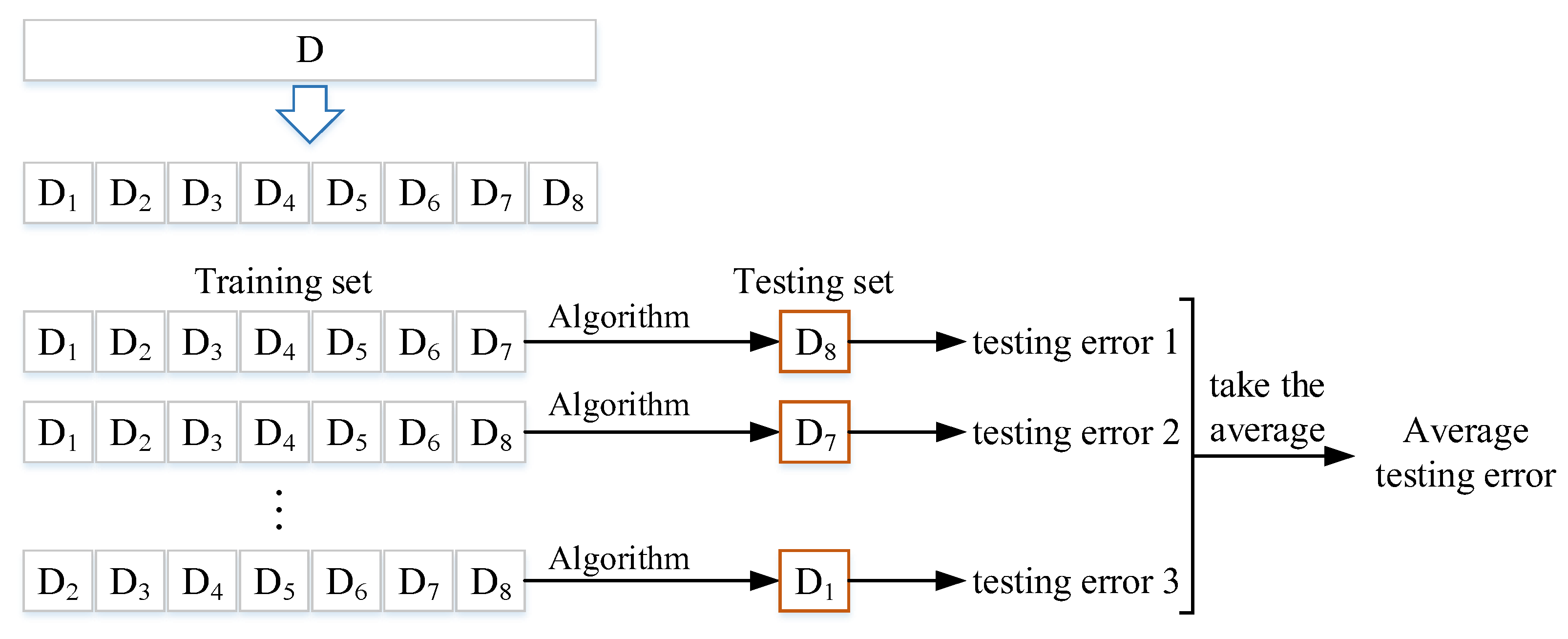
| Algorithm | Average Testing Error |
|---|---|
| GWO | 135.81 |
| PSO | 190.32 |
| GA | 205.14 |
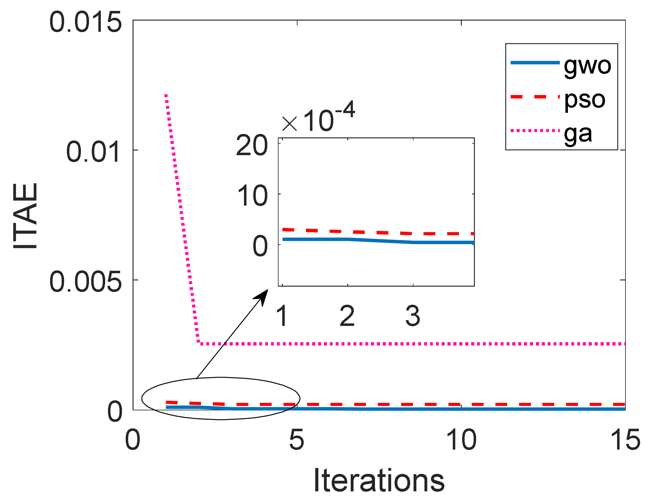
| Algorithm | Parameter Setting Time | Fitness Value | Number of Iterations |
|---|---|---|---|
| GWO | 64.86 s | 3.875 × 10⁻⁵ | 15 |
| PSO | 82.77 s | 2.15 × 10⁻⁴ | 15 |
| GA | 40.25 s | 2.55 × 10⁻³ | 15 |

| Parameters of ADRC | Algorithm | Parameters of ADRC | Algorithm | ||||
|---|---|---|---|---|---|---|---|
| GWO | PSO | GA | GWO | PSO | GA | ||
| r | 2.44 × 10⁻⁴ | 1 × 10⁻² | 9.87 × 10⁻² | b01 | 2.55 × 10² | 7.94 × 10³ | 4.58 × 10³ |
| h | 7.53 × 10³ | 3.11 × 10³ | 4.18 × 10³ | b02 | 6.48 × 10² | 3.73 × 10³ | 9.44 × 10³ |
| δ | 2.65 × 10³ | 2.78 × 10² | 5.9 × 10³ | b1 | 1.69 × 10³ | 7.5 × 10³ | 1.13 × 10² |
| hNLSEF | 2.15 × 10² | 7.47 × 10² | 3.76 × 10² | b5 | 2.85 × 10³ | 7.53 × 10³ | 8.86 × 10³ |
| b0 | 4.40 × 10³ | 1.67 × 10³ | 2.82 × 10³ | b2 | 0.034757 | 6.21 × 10³ | 0.0242 |
| d1 | 1.25 × 10³ | 1.16 × 10³ | 2.11 × 10³ | b3 | 0.09000 | 0.0500 | 0.0376 |
| d2 | 1.04 × 10³ | 5.4 × 10³ | 5.96 × 10³ | b4 | 0.015020 | 0.0500 | 0.0566 |
| d3 | 3.58 × 10³ | 3.61 × 10³ | 1.79 × 10³ | b6 | 0.016928 | 1 × 10⁻³⁵ | 0.0372 |
Publisher’s Note: MDPI stays neutral with regard to jurisdictional claims in published maps and institutional affiliations. |
© 2022 by the authors. Licensee MDPI, Basel, Switzerland. This article is an open access article distributed under the terms and conditions of the Creative Commons Attribution (CC BY) license (https://creativecommons.org/licenses/by/4.0/).
Share and Cite
Gao, B.; Guan, H.; Shen, W.; Ye, Y. Application of the Gray Wolf Optimization Algorithm in Active Disturbance Rejection Control Parameter Tuning of an Electro-Hydraulic Servo Unit. Machines 2022, 10, 599. https://doi.org/10.3390/machines10080599
Gao B, Guan H, Shen W, Ye Y. Application of the Gray Wolf Optimization Algorithm in Active Disturbance Rejection Control Parameter Tuning of an Electro-Hydraulic Servo Unit. Machines. 2022; 10(8):599. https://doi.org/10.3390/machines10080599
Chicago/Turabian StyleGao, Bingwei, Hao Guan, Wei Shen, and Yongtai Ye. 2022. "Application of the Gray Wolf Optimization Algorithm in Active Disturbance Rejection Control Parameter Tuning of an Electro-Hydraulic Servo Unit" Machines 10, no. 8: 599. https://doi.org/10.3390/machines10080599