
Advanced Motor Control for Improving the Trajectory Tracking Accuracy of a Low-Cost Mobile Robot
 , , and
Abstract
:1. Introduction
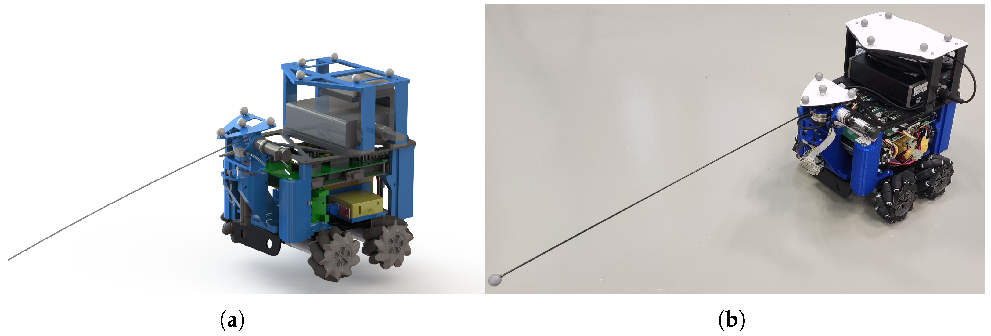
2. Robot Setup
- The chassis, which is equipped with four DC motors with incremental encoders and reduction gears that drive four mecanum wheels (Swedish wheels with rollers at ). The motors (model GM25-370-24140-75-14.5D10) operate at a voltage control signal within ±9 V, and their reduction gear ratio is 1:75. The encoder resolution is 4 pulses per turn of the motor axle, which corresponds to around 300 pulses per turn of the omni wheel. Hence, the wheel angular position can be measured with an accuracy of .
- A National Instruments Field Programmable Gate Array (FPGA) compactRIO control board, model sbRIO-9631. This card is used to command the motor controllers of the robot (four for the MWMR and two for the whisker), read sensor measurements (encoders and force-torque sensor) and communicate with a host computer via .
- Four servo controller boards Maxon ESCON Module . These controllers are mounted on a shield board connected on top of the FPGA and close the inner current loops of the motors, so that the electrical model of each motor can be reduced to a Thevenin equivalent, and the electrical dynamics can be neglected because they are much faster than the mechanical dynamics. They receive the control signals from the FPGA through digital ports and provide the power needed by the motors to operate.
- A router (model GL.iNet GL-MT300N-V2). This is used to establish wireless communication between the FPGA and an external host computer using a protocol.
- Two 3500 mAh, 3-cell (11.1 V) batteries connected in series to deliver nominal 22.2 V. They supply the power to the FPGA, the ESCON modules and, using step-down converter from 22 to 5 V, the router.
3. Modeling and Identification
3.1. Analytical Model
3.2. Identification of the Linear Model
3.3. Identification of Non-Linearities
3.3.1. Friction Phenomena
- The viscous friction, which is proportional to through the viscous friction coefficient . It is a linear effect that has already been included in the linear model (7).
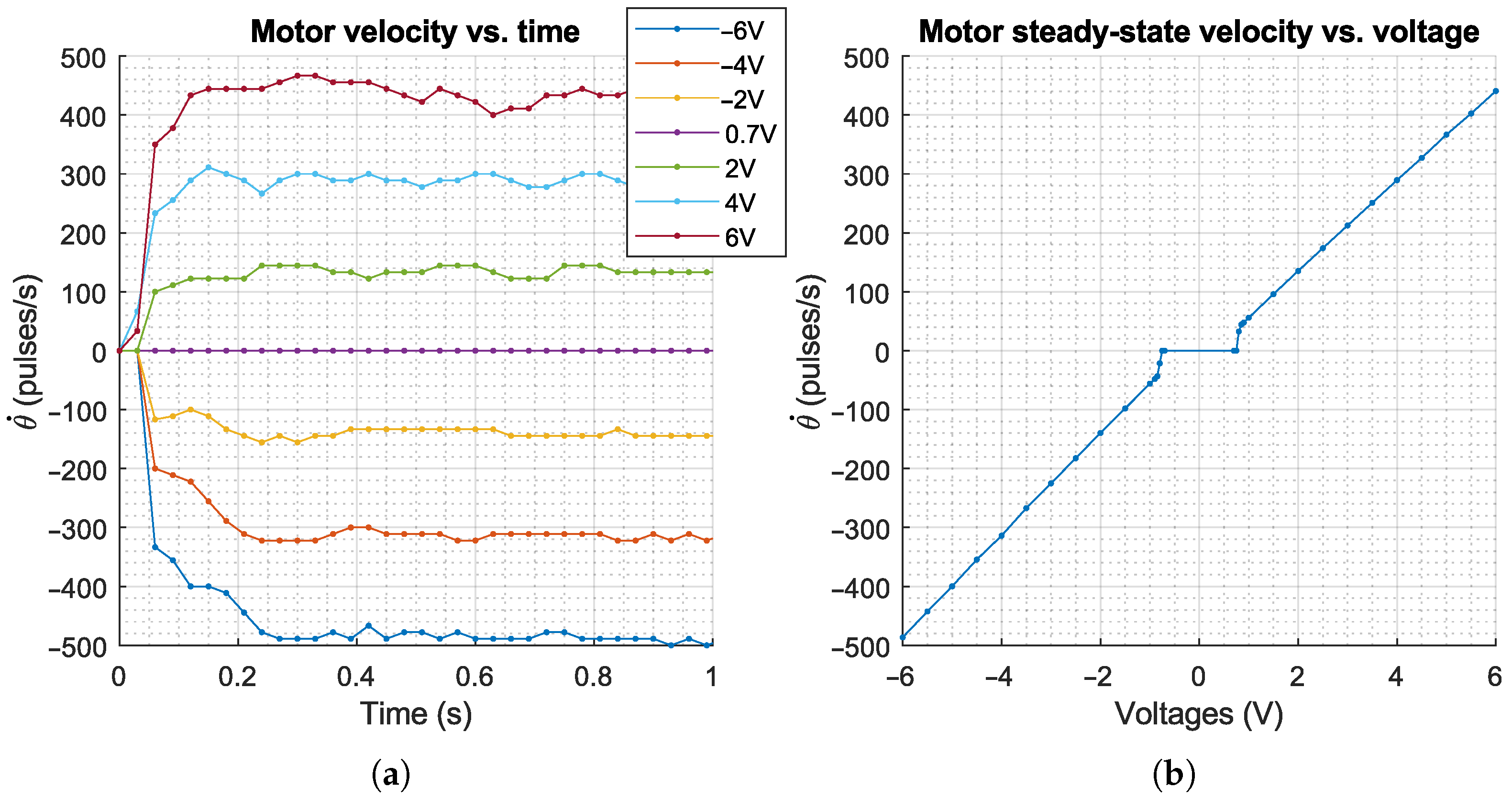
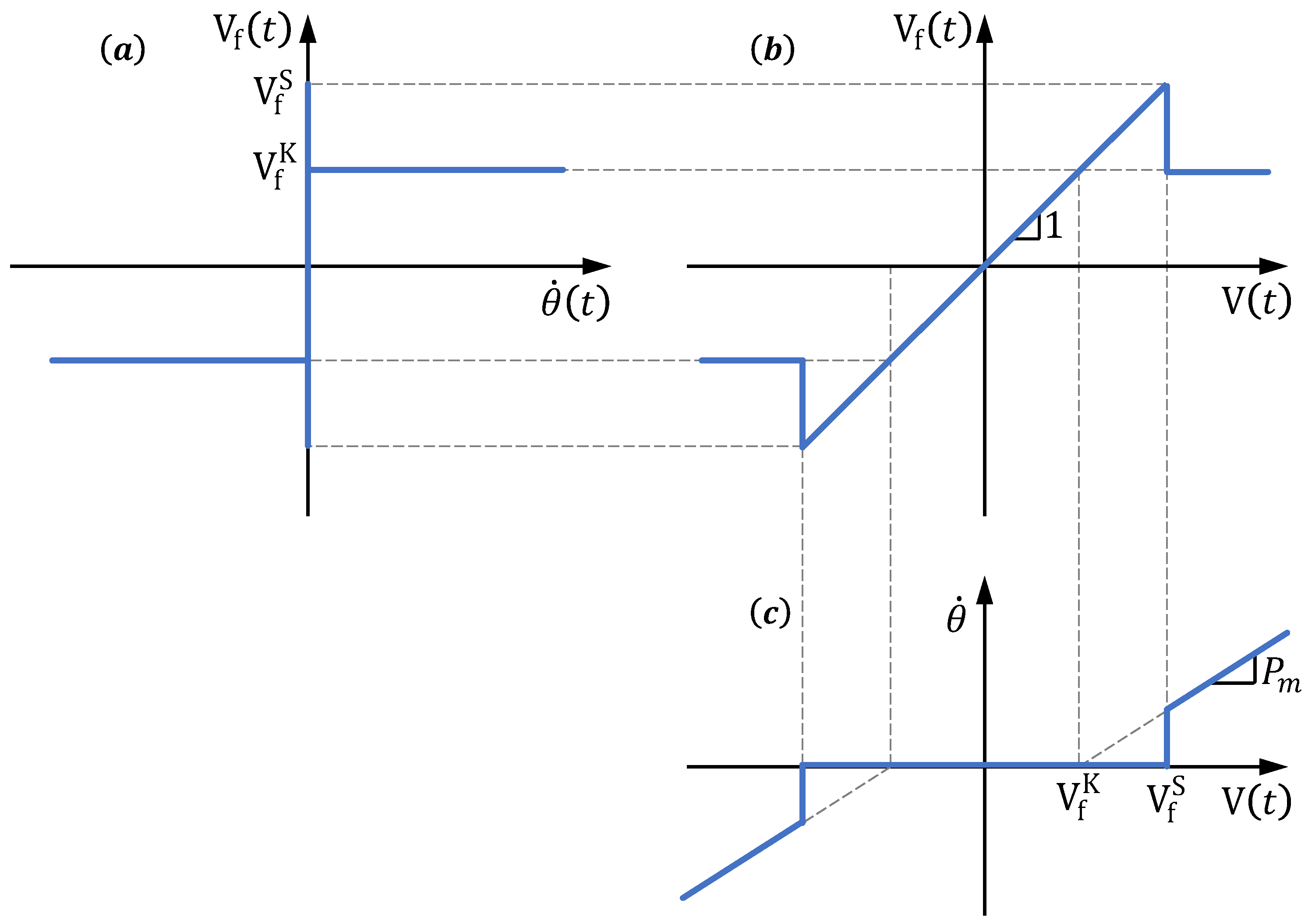
- The static friction (stiction) and break-away force. This effect has been observed in Figure 3b, where a discontinuity in appears near ±1 V. It occurs when the applied motor torque —expressed in terms of the supplied voltage as expressed in (3)—is lower than the maximum torque generated by the static motor and gearbox internal frictions. This causes the motor to remain stuck without movement. Once is big enough, the motor starts moving. That is the point where the break-away force is overcome. This phenomenon defines a region called motor dead-zone in which the motor remains stuck when applying torques lower than the break-away torque.
- The Coulomb friction. This friction force appears when the motor is running with non-zero velocity. Its magnitude, which is denoted as the kinetic friction, is constant and its direction is opposite to the motion.
- The Stribeck friction, which is the transition between the stiction and the Coulomb friction. When overcomes the break-away value, the motor starts running at very low speed and the friction value decreases rapidly. The rapid decrease in the friction value causes an increase in motor velocity, what again causes a friction decrease. This is repeated until the Coulomb friction value is reached. This phenomenon is continuous, depends on the velocity, and occurs in a very short range of velocities.
3.3.2. Saturation
3.3.3. Encoder Resolution
3.4. Identification Results
3.5. Complete Model of the System
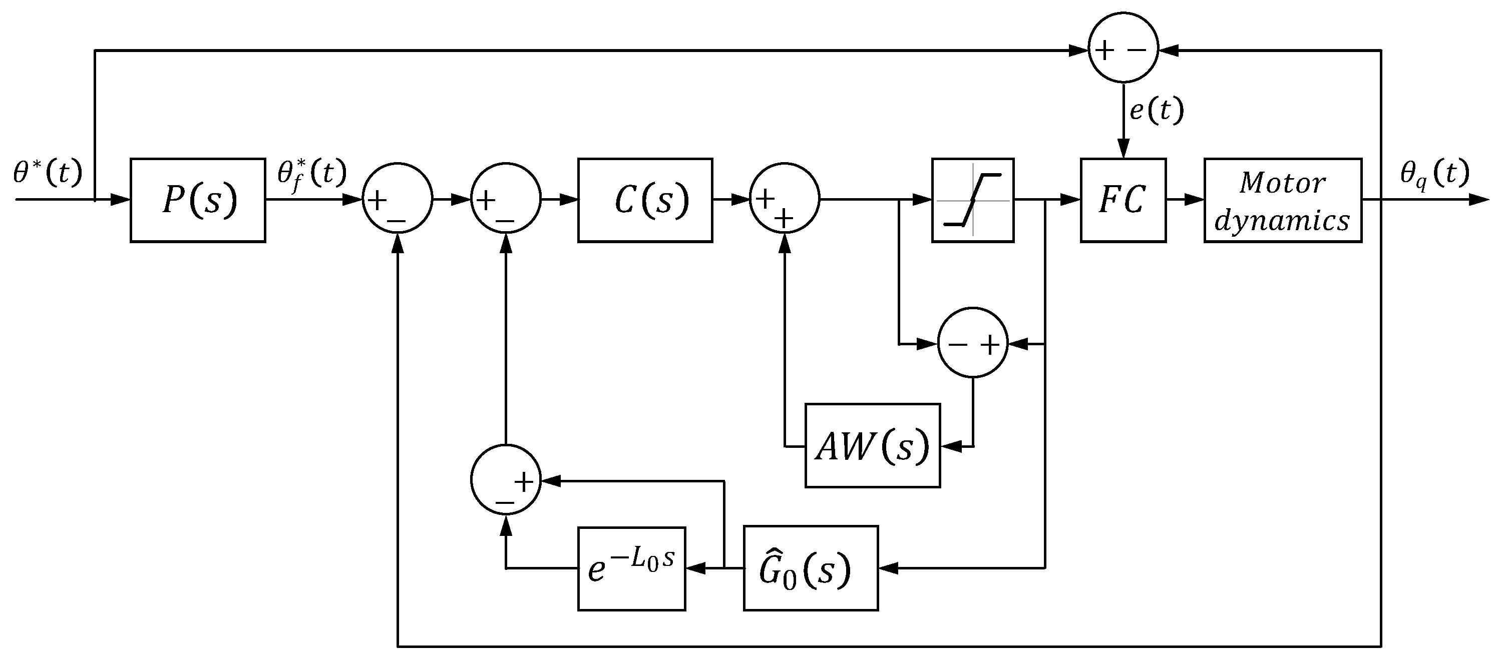
4. Control Scheme Design
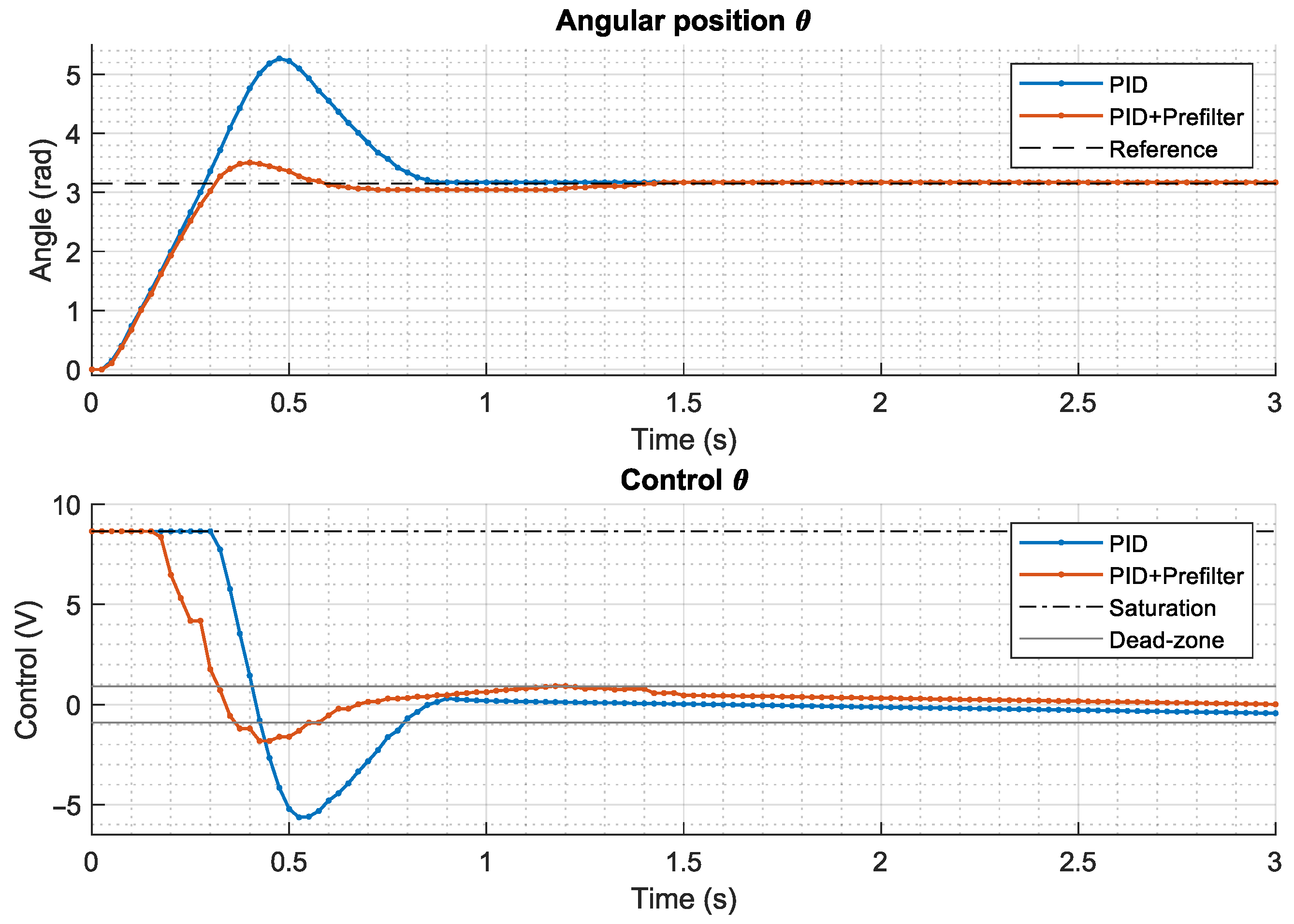
4.1. PID Regulator with Prefilter
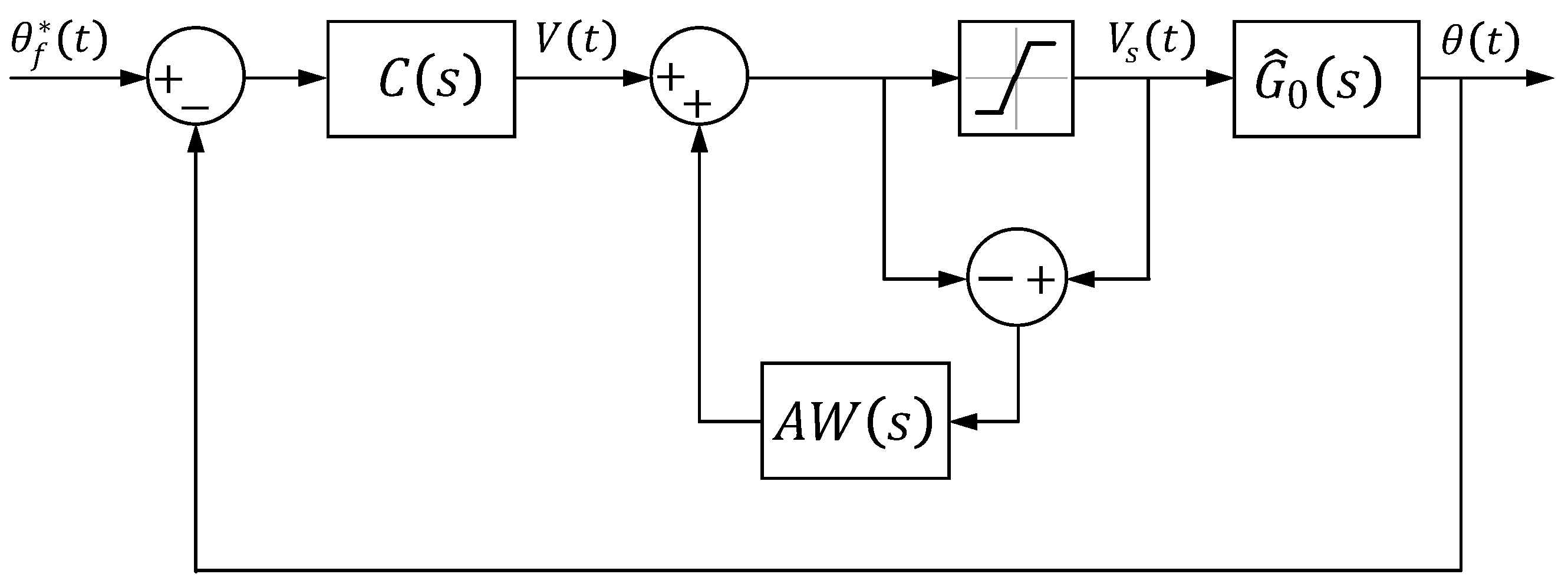
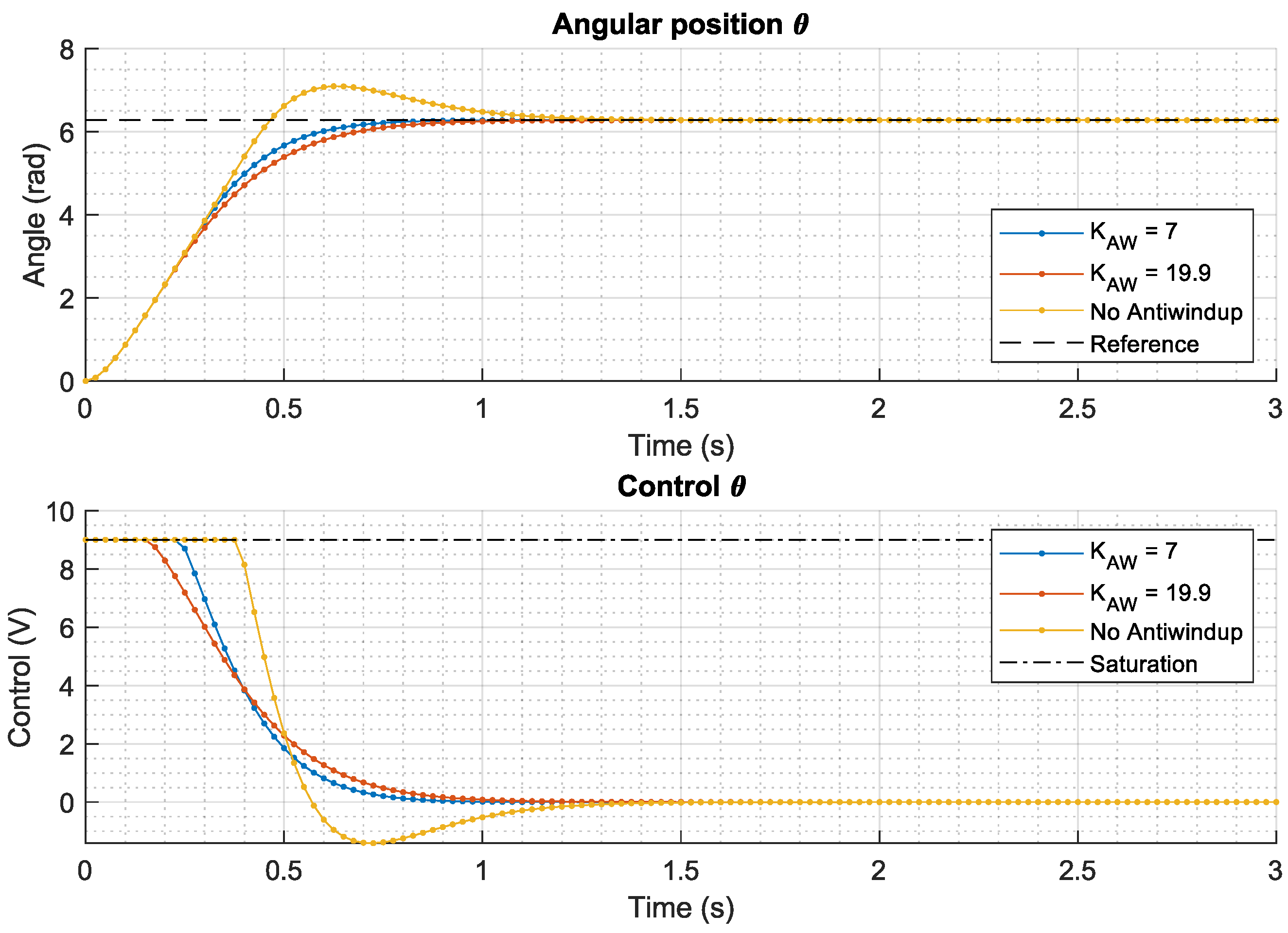
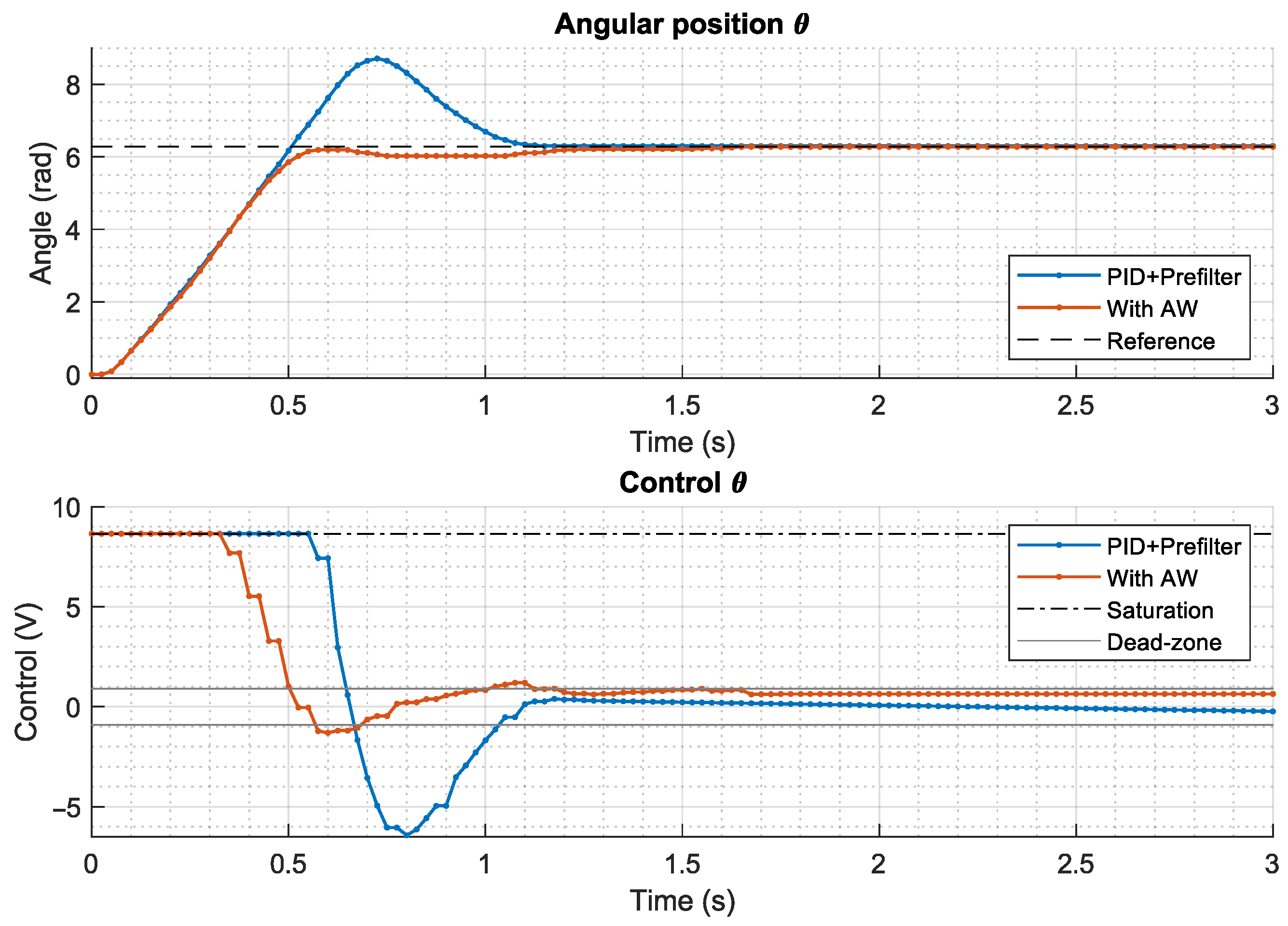
4.2. Antiwindup
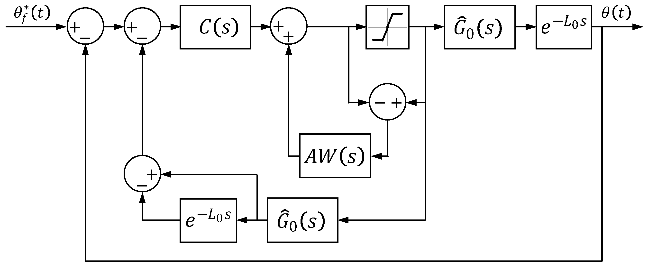
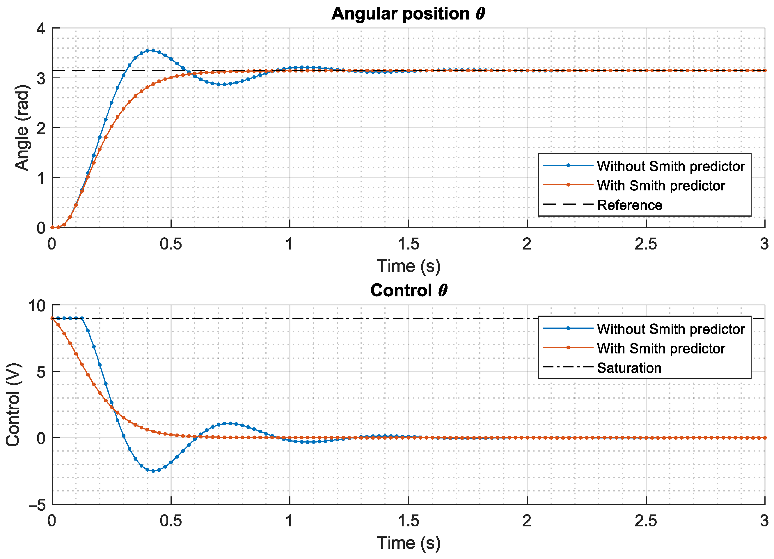
4.3. Smith Predictor
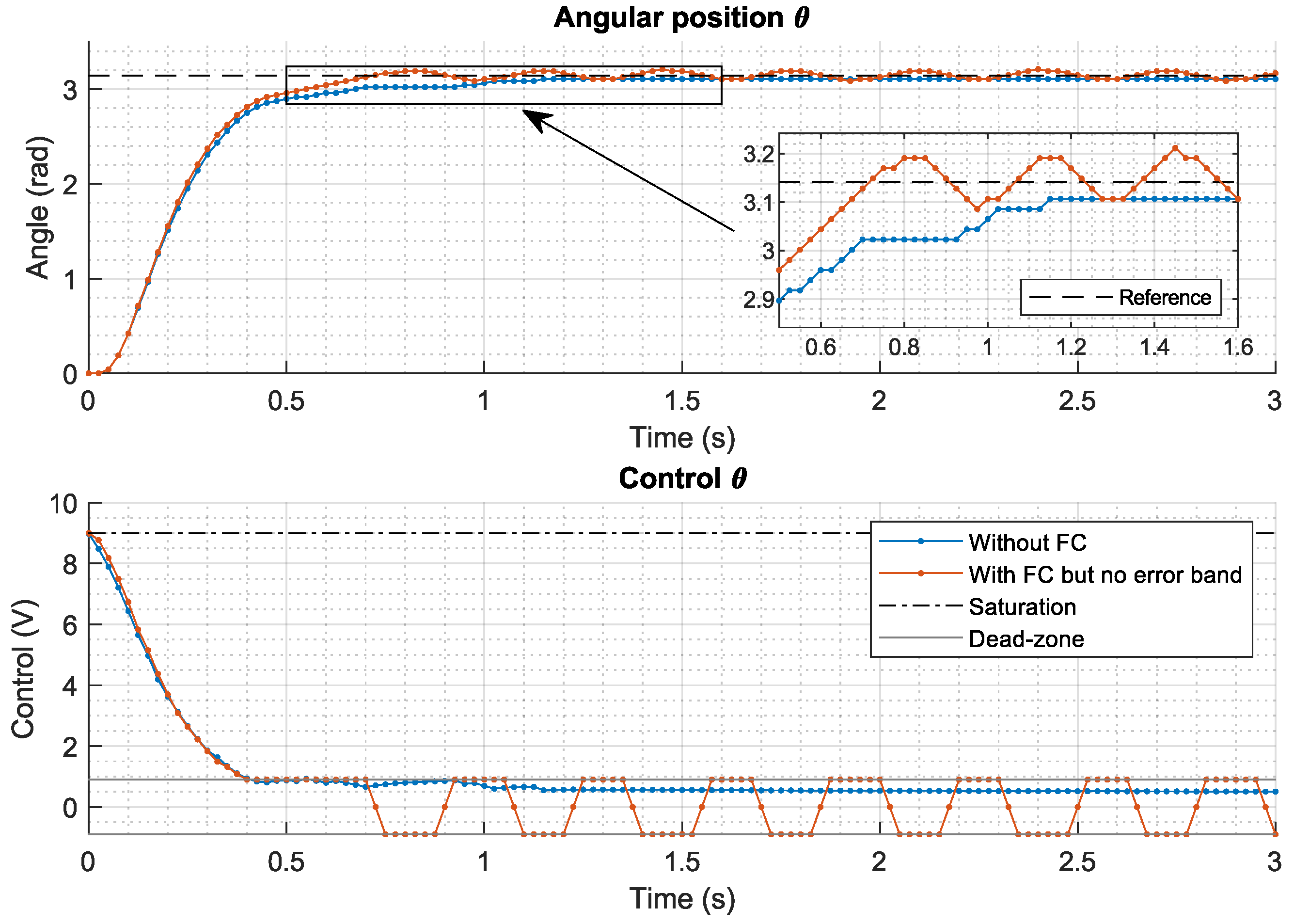
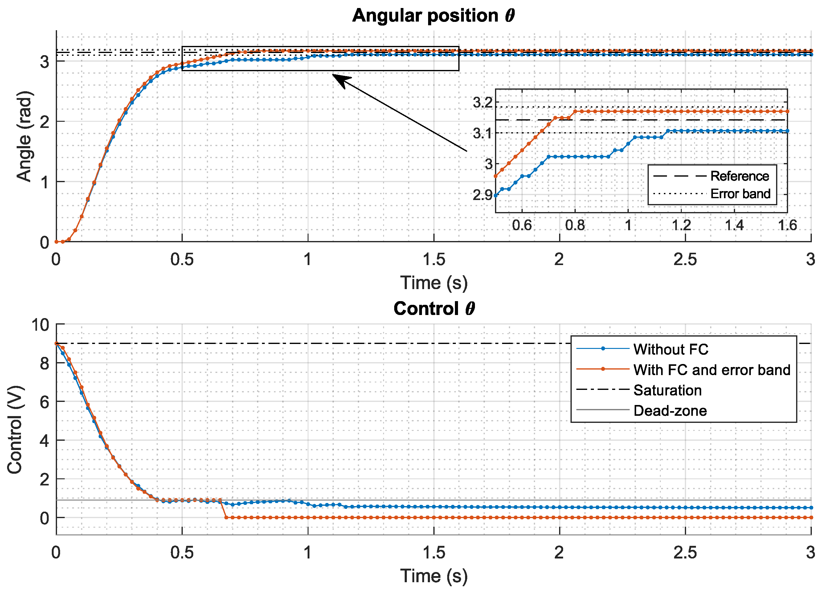
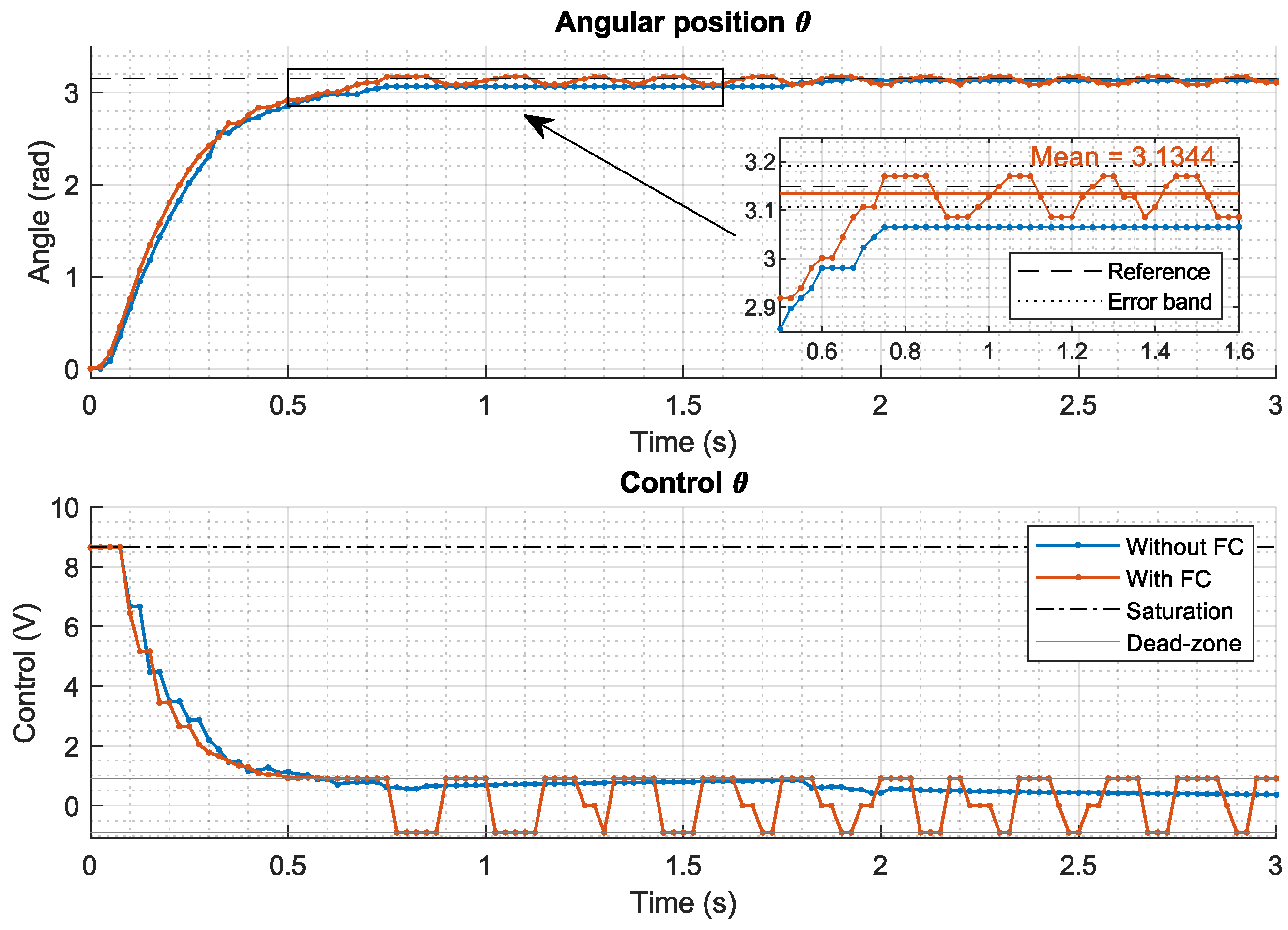
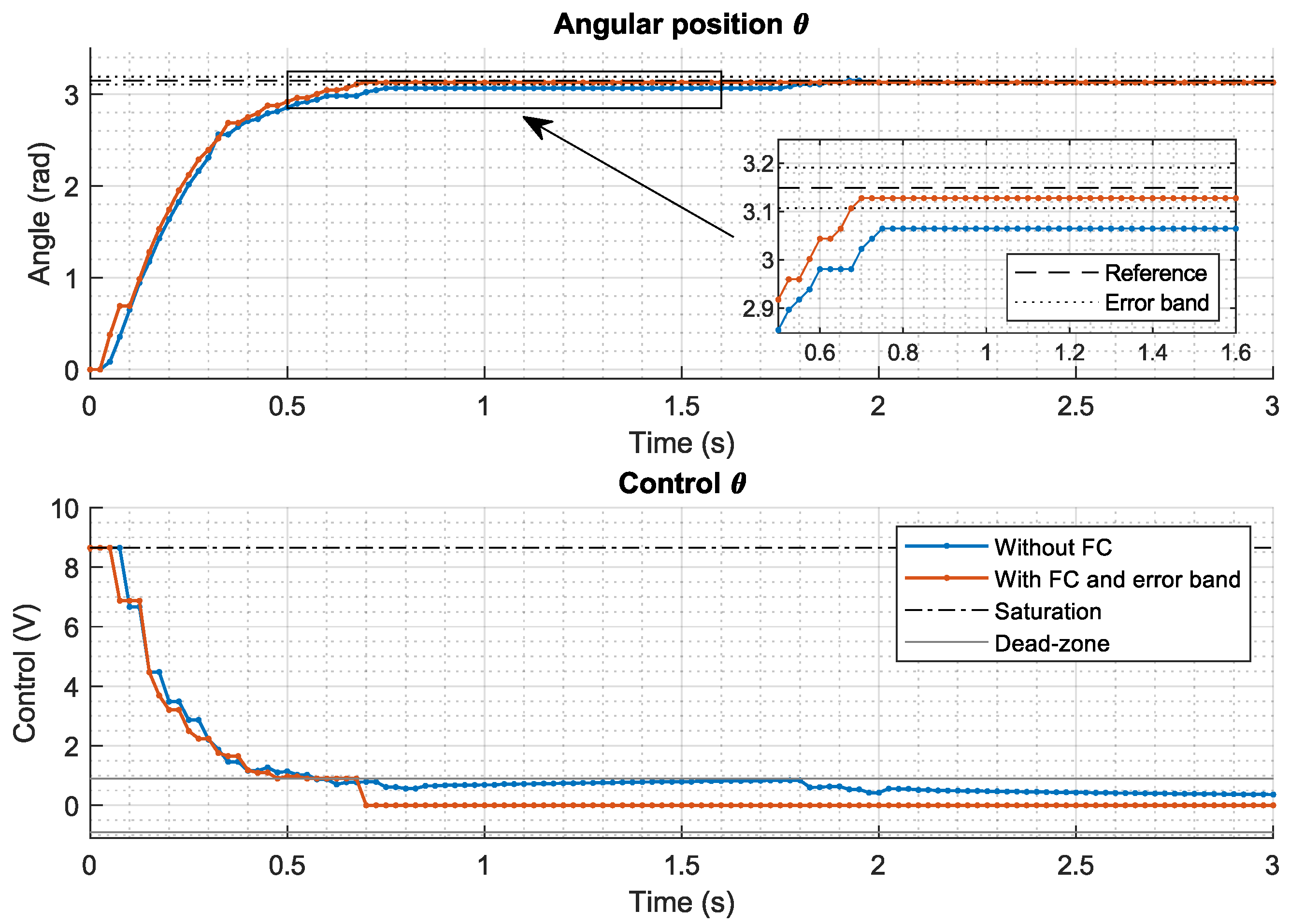
4.4. Friction Compensator
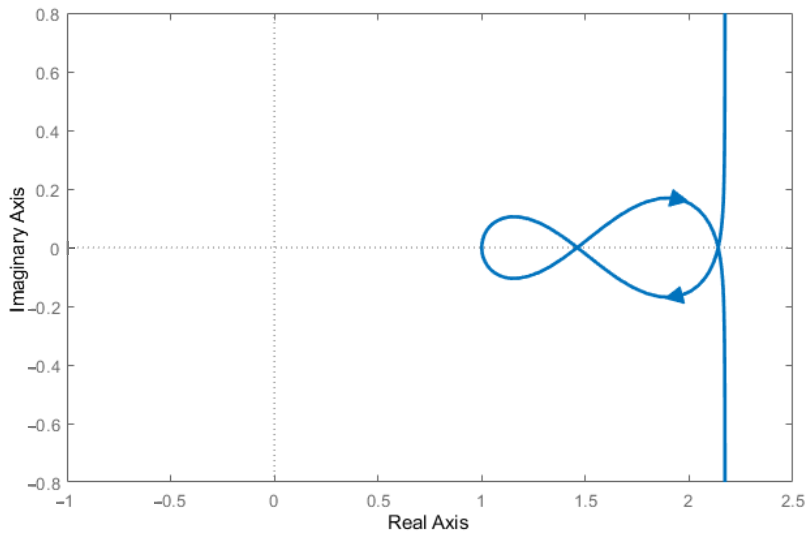
4.5. Stability Analysis
5. Results
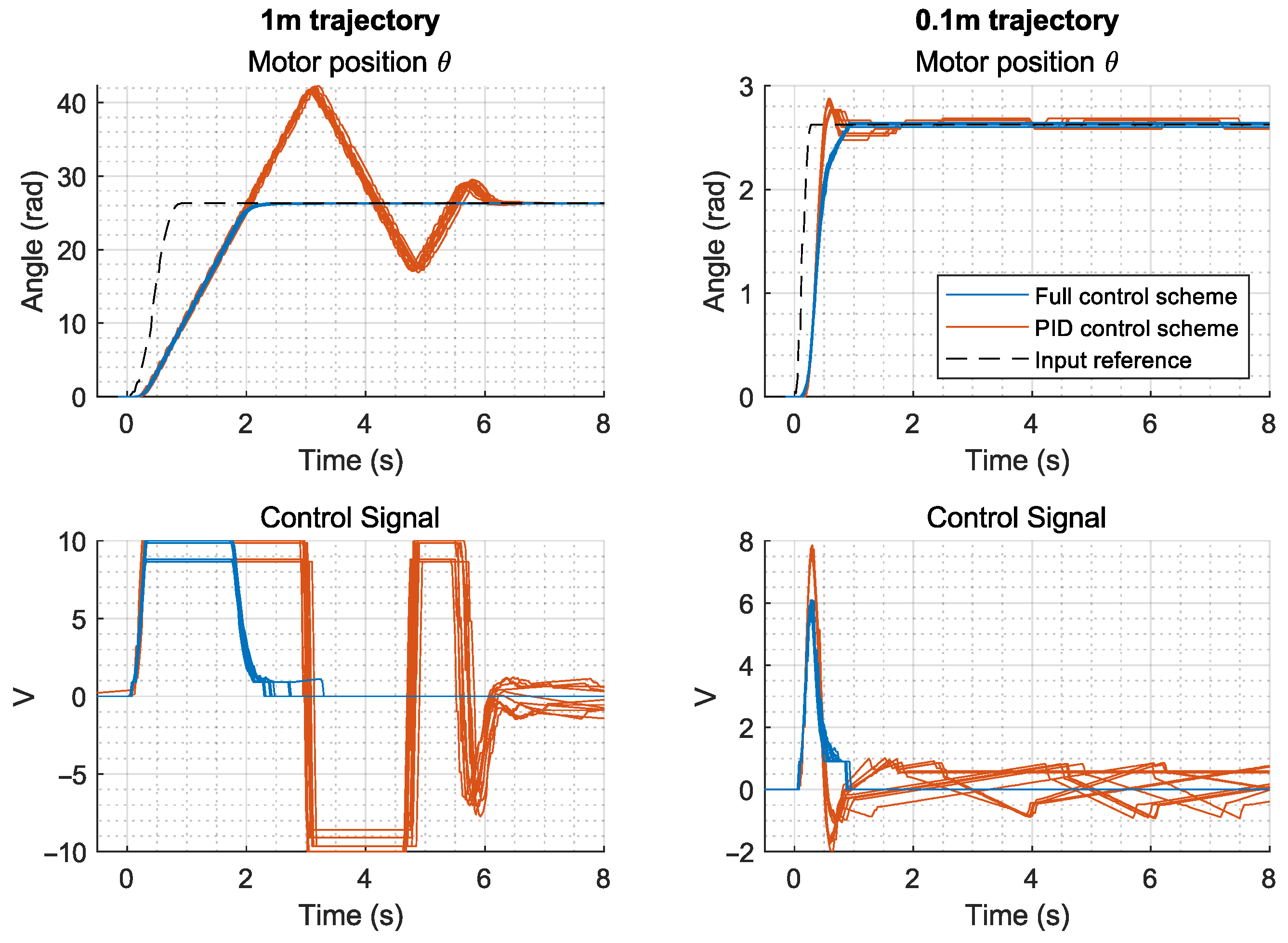
5.1. Motor Control System
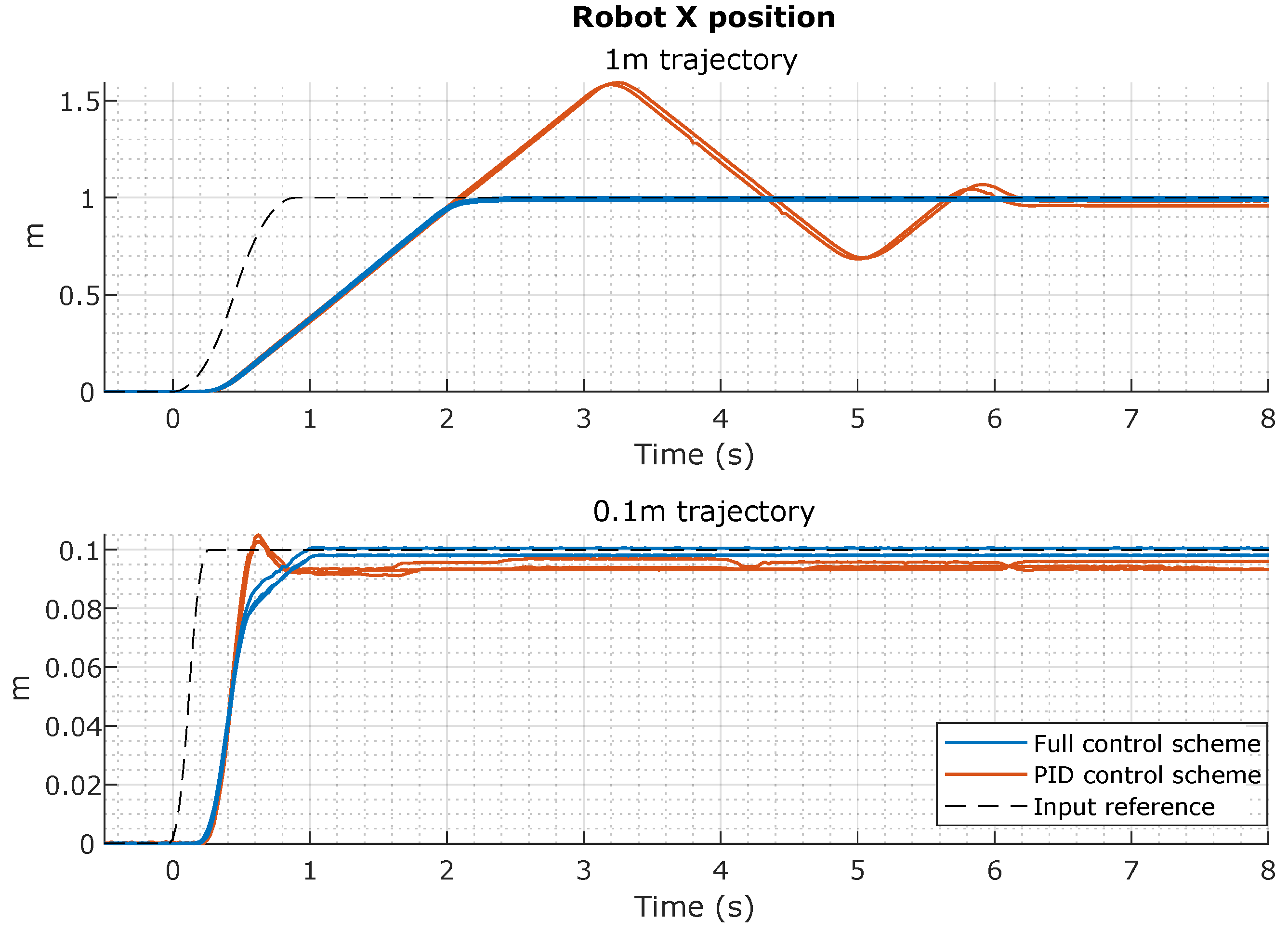
5.2. Robot Trajectory Tracking
6. Conclusions
Author Contributions
Funding
Informed Consent Statement
Data Availability Statement
Conflicts of Interest
Abbreviations
| PID | Proportional–Integral–Derivative controller |
| DC | Direct-Current |
| MWMR | Mecanum-Wheeled Mobile Robot |
| dof | degrees-of-freedom |
| PTP | Point-To-Point |
| HID | Hardware-Induced Delay |
| ACP | Advanced Control Process |
| FPGA | Field Programmable Gate Array |
| FB | Friction Block |
| ER | Encoder Resolution block |
| FC | Friction Compensator |
| SPR | Strictly Positive Real |
| Motor torque | |
| Motor torque without reduction gear | |
| n | Reduction gear ratio |
| Motor electromechanical constant | |
| V | Input voltage |
| Motor inertia | |
| Robot inertia | |
| J | Total inertia |
| Motor angle | |
| Motor viscous friction | |
| Non-linear motor friction | |
| Motor transfer function between V and | |
| A, B | Motor identified parameters |
| Motor transfer function between V and motor angular velocity | |
| Settling time | |
| Relation between applied voltage and angular velocity in steady-state | |
| L | Time delay |
| G | Motor transfer function including time delay |
| Coulomb friction voltage | |
| Stiction brake-away equivalent voltage | |
| Kinetic friction equivalent voltage | |
| Load torque in terms of voltage | |
| Motor saturation voltage | |
| Encoder measure | |
| Saturated input voltage | |
| Motor nominal transfer function between V and | |
| , | Motor nominal identified parameters |
| Nominal time delay | |
| Motor nominal transfer function between V and | |
| Motor desired trajectory | |
| P | Prefilter |
| Output signal of the prefilter | |
| C | PID controller |
| , , , | PID parameters |
| , , , , p | Poles of the system |
| Closed loop transfer function of the system without prefilter | |
| Closed loop transfer function of the system with prefilter | |
| Antiwindup transfer function | |
| N, K, , | PID parameters in standard form |
| Antiwindup coefficient | |
| Compensated input voltage | |
| Control signal modified by the antiwindup | |
| Minimum voltage provided to the motor | |
| Minimum motor angular displacement defining the error band | |
| e | Error signal |
| F, H, Q, , G, , D | Vectors and matrices of the state-space system of PID and antiwindup |
| Linearized PID and antiwindup system | |
| W, | Functions of the linearized system |
References
- de Wit, C.C.; Lischinsky, P. Adaptive Friction Compensation with Dynamic Friction Model. IFAC Proc. Vol. 1996, 29, 2078–2083. [Google Scholar] [CrossRef]
- Bona, B.; Indri, M. Friction compensation in robotics: An overview. In Proceedings of the 44th IEEE Conference on Decision and Control (CDC-ECC ’05), Seville, Spain, 15 December 2005; pp. 4360–4367. [Google Scholar] [CrossRef]
- Conceição, A.S.; Moreira, P.A.; Costa, P.J. Practical approach of modeling and parameters estimation for omnidirectional mobile robots. IEEE/ASME Trans. Mechatron. 2009, 14, 377–381. [Google Scholar] [CrossRef]
- Rubaai, A.; Kotaru, R. Online Identification and Control of a DC Motor Using Learning Adaptation of Neural Networks. IEEE Trans. Ind. Appl. 2000, 36, 935. [Google Scholar] [CrossRef]
- Ramos, F.; Feliu, V. New online payload identification for flexible robots. Application to adaptive control. J. Sound Vib. 2008, 315, 34–57. [Google Scholar] [CrossRef]
- Mamani, G.; Becedas, J.; Feliu-Batlle, V.; Sira-Ramírez, H. Open-and closed-loop algebraic identification method for adaptive control of DC motors. Int. J. Adapt. Control Signal Process. 2009, 23, 1097–1103. [Google Scholar] [CrossRef]
- Hendzel, Z.; Kolodziej, M. Robust Tracking Control of Omni-Mecanum Wheeled Robot. Adv. Intell. Syst. Comput. 2021, 1390, 219–229. [Google Scholar] [CrossRef]
- Tu, K.Y. A linear optimal tracker designed for omnidirectional vehicle dynamics linearized based on kinematic equations. Robotica 2010, 28, 1033–1043. [Google Scholar] [CrossRef]
- Bouzoualegh, S.; Guechi, E.H.; Kelaiaia, R. Model Predictive Control of a Differential-Drive Mobile Robot. Acta Univ. Sapientiae Electr. Mech. Eng. 2018, 10, 20–41. [Google Scholar] [CrossRef] [Green Version]
- Moreno-Caireta, I.; Celaya, E.; Ros, L. Model Predictive Control for a Mecanum-wheeled Robot Navigating among Obstacles. IFAC-PapersOnLine 2021, 54, 119–125. [Google Scholar] [CrossRef]
- Ovalle, L.; Ríos, H.; Llama, M.; Santibáñez, V.; Dzul, A. Omnidirectional mobile robot robust tracking: Sliding-mode output-based control approaches. Control Eng. Pract. 2019, 85, 50–58. [Google Scholar] [CrossRef]
- Szeremeta, M.; Szuster, M. Neural Tracking Control of a Four-Wheeled Mobile Robot with Mecanum Wheels. Appl. Sci. 2022, 12, 5322. [Google Scholar] [CrossRef]
- Dhaouadi, R.; Hatab, A.A. Dynamic Modelling of Differential-Drive Mobile Robots using Lagrange and Newton-Euler Methodologies: A Unified Framework. Adv. Robot. Autom. 2013, 2, 1–7. [Google Scholar] [CrossRef] [Green Version]
- Hendzel, Z.; Rykała, Ł. Modelling of dynamics of a wheeled mobile robot with mecanum wheels with the use of lagrange equations of the second kind. Int. J. Appl. Mech. Eng. 2017, 22, 81–99. [Google Scholar] [CrossRef] [Green Version]
- Alakshendra, V.; Chiddarwar, S. Adaptive robust control of Mecanum-wheeled mobile robot with uncertainties. Nonlinear Dyn. 2017, 87, 2147–2169. [Google Scholar] [CrossRef]
- Ruderman, M.; Iwasaki, M. Observer of nonlinear friction dynamics for motion control. IEEE Trans. Ind. Electron. 2015, 62, 5941–5949. [Google Scholar] [CrossRef]
- Comasolivas, R.; Quevedo, J.; Escobet, T.; Escobet, A.; Romera, J. Modeling and Robust Low Level Control of an Omnidirectional Mobile Robot. J. Dyn. Syst. Meas. Control Trans. ASME 2017, 139, 041011. [Google Scholar] [CrossRef]
- Shao, K.; Tang, R.; Xu, F.; Wang, X.; Zheng, J. Adaptive sliding mode control for uncertain Euler–Lagrange systems with input saturation. J. Frankl. Inst. 2021, 358, 8356–8376. [Google Scholar] [CrossRef]
- Wu, W. DC motor parameter identification using speed step responses. Model. Simul. Eng. 2012, 2012, 189757. [Google Scholar] [CrossRef] [Green Version]
- Rodriguez, A.S.M.; Hosseini, M.; Paik, J. Hybrid Control Strategy for Force and Precise End Effector Positioning of a Twisted String Actuator. IEEE/ASME Trans. Mechatron. 2021, 26, 2791–2802. [Google Scholar] [CrossRef]
- Gruzman, M.; Weber, H.I.; Menegaldo, L.L. Time Domain Simulation of a Target Tracking System with Backlash Compensation. Math. Probl. Eng. 2010, 2010, 973482. [Google Scholar] [CrossRef]
- Santos, J.; Conceição, A.G.; Santos, T.L. Trajectory tracking of Omni-directional Mobile Robots via Predictive Control plus a Filtered Smith Predictor. IFAC-PapersOnLine 2017, 50, 10250–10255. [Google Scholar] [CrossRef]
- Castillo-Berrio, C.F.; Feliu-Batlle, V. Vibration-free position control for a two degrees of freedom flexible-beam sensor. Mechatronics 2015, 27, 1–12. [Google Scholar] [CrossRef]
- Mérida-Calvo, L.; Feliu-Talegón, D.; Feliu-Batlle, V. Improving the Detection of the Contact Point in Active Sensing Antennae by Processing Combined Static and Dynamic Information. Sensors 2021, 21, 1808. [Google Scholar] [CrossRef] [PubMed]
- Ogata, K. Modern Control Engineering; Prentice Hall: Upper Saddle River, NJ, USA, 2010; Volume 5. [Google Scholar]
- Olsson, H.; Åström, K.J.; Canudas De Wit, C.; Gäfvert, M.; Lischinsky, P. Friction Models and Friction Compensation. Eur. J. Control 1998, 4, 176–195. [Google Scholar] [CrossRef] [Green Version]
- Pennestrì, E.; Rossi, V.; Salvini, P.; Valentini, P.P. Review and comparison of dry friction force models. Nonlinear Dyn. 2016, 83, 1785–1801. [Google Scholar] [CrossRef]
- Virgala, I.; Frankovský, P.; Kenderová, M. Friction Effect Analysis of a DC Motor. Am. J. Mech. Eng. 2013, 1, 1–5. [Google Scholar] [CrossRef] [Green Version]
- Olejnik, P.; Awrejcewicz, J.; Fečkan, M. Modeling, Analysis and Control of Dynamical Systems with Friction and Impacts; World Scientific Publishing Co.: Singapore, 2017; pp. 1–262. [Google Scholar] [CrossRef]
- Åström, T.K. PID Controllers: Theory, Design, and Tunning, 2nd ed.; Instrument Society of America (ISA): Research Triangle Park, NC, USA, 1995. [Google Scholar]
- Bahill, A.T. Simple Adaptive Smith-Predictor for Controlling Time-Delay Systems. IEEE Control Syst. Mag. 1983, 3, 16–22. [Google Scholar] [CrossRef]
- Rundqwist, L. Anti-reset Windup for PID Controllers. IFAC Proc. Vol. 1990, 23, 453–458. [Google Scholar] [CrossRef]
- Åström, K.J.; Wittenmark, B. Computer-Controlled Systems: Theory and Design; Courier Corporation: Englewood Cliffs, NJ, USA, 2013. [Google Scholar]
- Narendra, K.S.; Taylor, J.H. Frequency Domain Criteria for Absolute Stability; Academic Press, Inc.: New York, NY, USA, 1973. [Google Scholar]
- Popov, V. Absolute stability of nonlinear systems of automatic control. Autom. Remote Control 1962, 22, 857–875. [Google Scholar]
- Cho, Y.S.; Narendra, K.S. An Off-Axis Circle Criterion for the Stability of Feedback Systems with a Monotonic Nonlinearity. IEEE Trans. Autom. Control 1968, 13, 413–416. [Google Scholar] [CrossRef]


| Parameters | A | B | L (s) | (V) | (V) |
|---|---|---|---|---|---|
| Mean value | 1631.32 | 19.97 | 0.0539 | 0.85 | 0.2898 |
| S. deviation | 68.66 | 0.83 | 0.004 | 0.00 | 0.0163 |
| % variance | 9.89% | 10.81% | 14.44% | 0% | 9.19% |
Disclaimer/Publisher’s Note: The statements, opinions and data contained in all publications are solely those of the individual author(s) and contributor(s) and not of MDPI and/or the editor(s). MDPI and/or the editor(s) disclaim responsibility for any injury to people or property resulting from any ideas, methods, instructions or products referred to in the content. |
© 2022 by the authors. Licensee MDPI, Basel, Switzerland. This article is an open access article distributed under the terms and conditions of the Creative Commons Attribution (CC BY) license (https://creativecommons.org/licenses/by/4.0/).
Share and Cite
Mérida-Calvo, L.; Rodríguez, A.S.-M.; Ramos, F.; Feliu-Batlle, V. Advanced Motor Control for Improving the Trajectory Tracking Accuracy of a Low-Cost Mobile Robot. Machines 2023, 11, 14. https://doi.org/10.3390/machines11010014
Mérida-Calvo L, Rodríguez AS-M, Ramos F, Feliu-Batlle V. Advanced Motor Control for Improving the Trajectory Tracking Accuracy of a Low-Cost Mobile Robot. Machines. 2023; 11(1):14. https://doi.org/10.3390/machines11010014
Chicago/Turabian StyleMérida-Calvo, Luis, Andrés San-Millán Rodríguez, Francisco Ramos, and Vicente Feliu-Batlle. 2023. "Advanced Motor Control for Improving the Trajectory Tracking Accuracy of a Low-Cost Mobile Robot" Machines 11, no. 1: 14. https://doi.org/10.3390/machines11010014