
Robust Reduced-Order Active Disturbance Rejection Control Method: A Case Study on Speed Control of a One-Dimensional Gimbal

 ,
,
Abstract
:1. Introduction
2. ADRC Algorithm
2.1. Classical ADRC Algorithm
2.2. Reduced-Order ADRC Algorithm
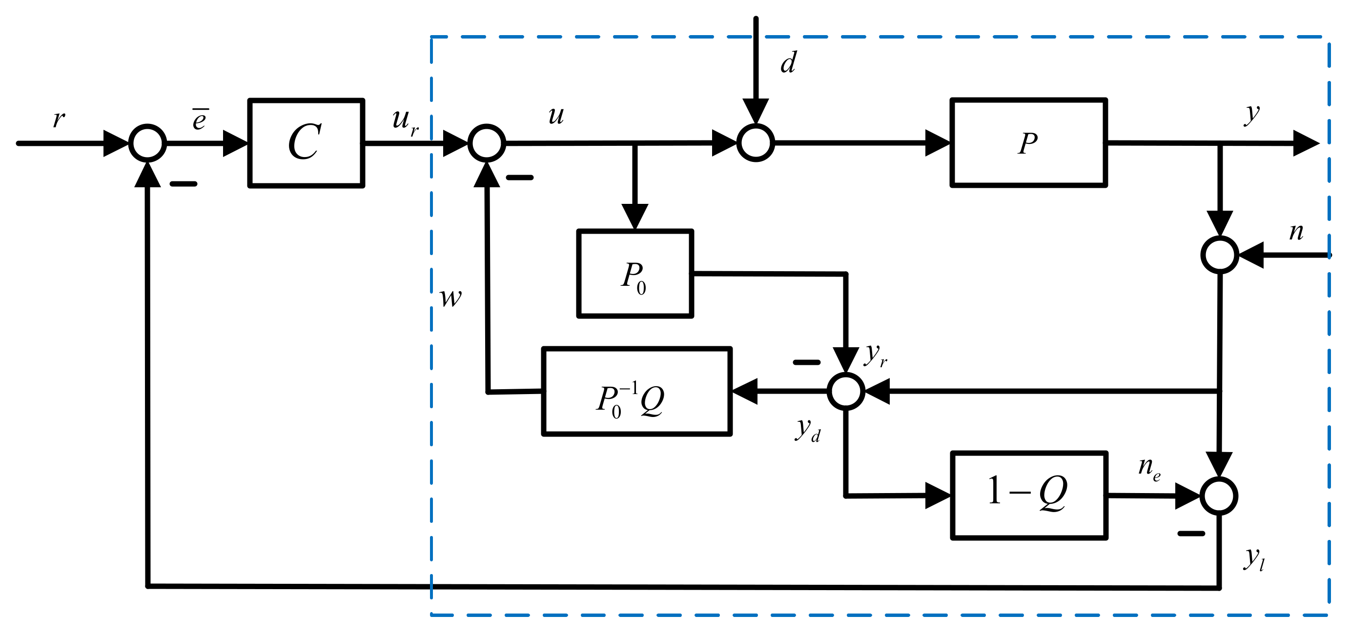
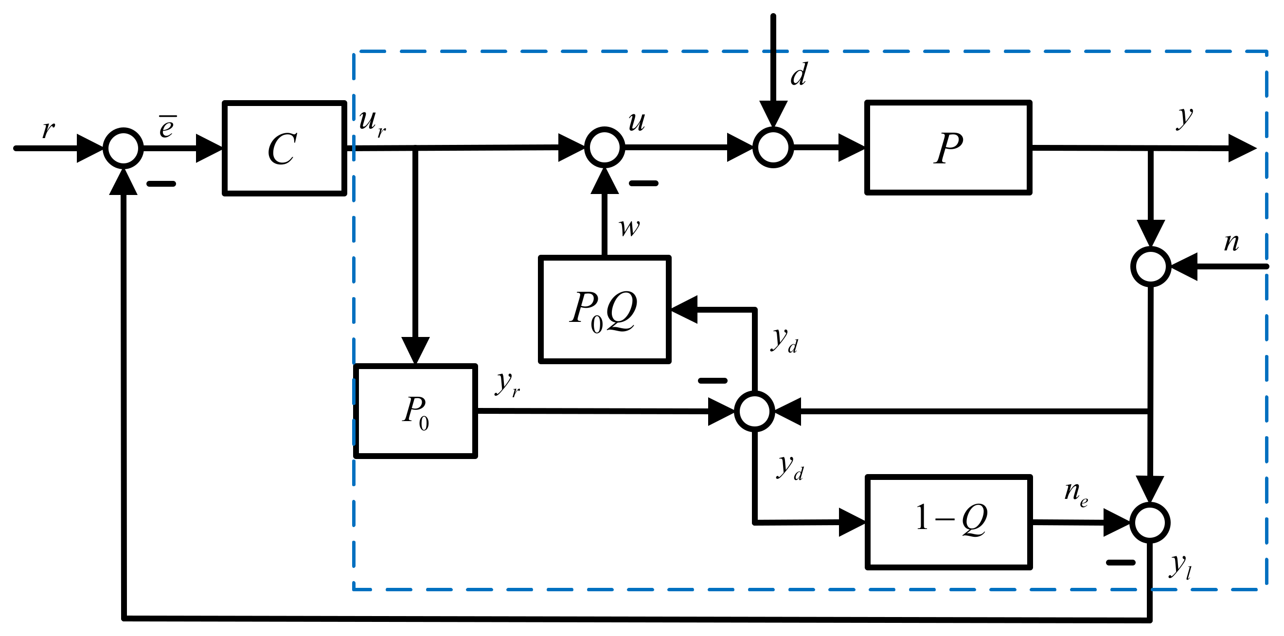
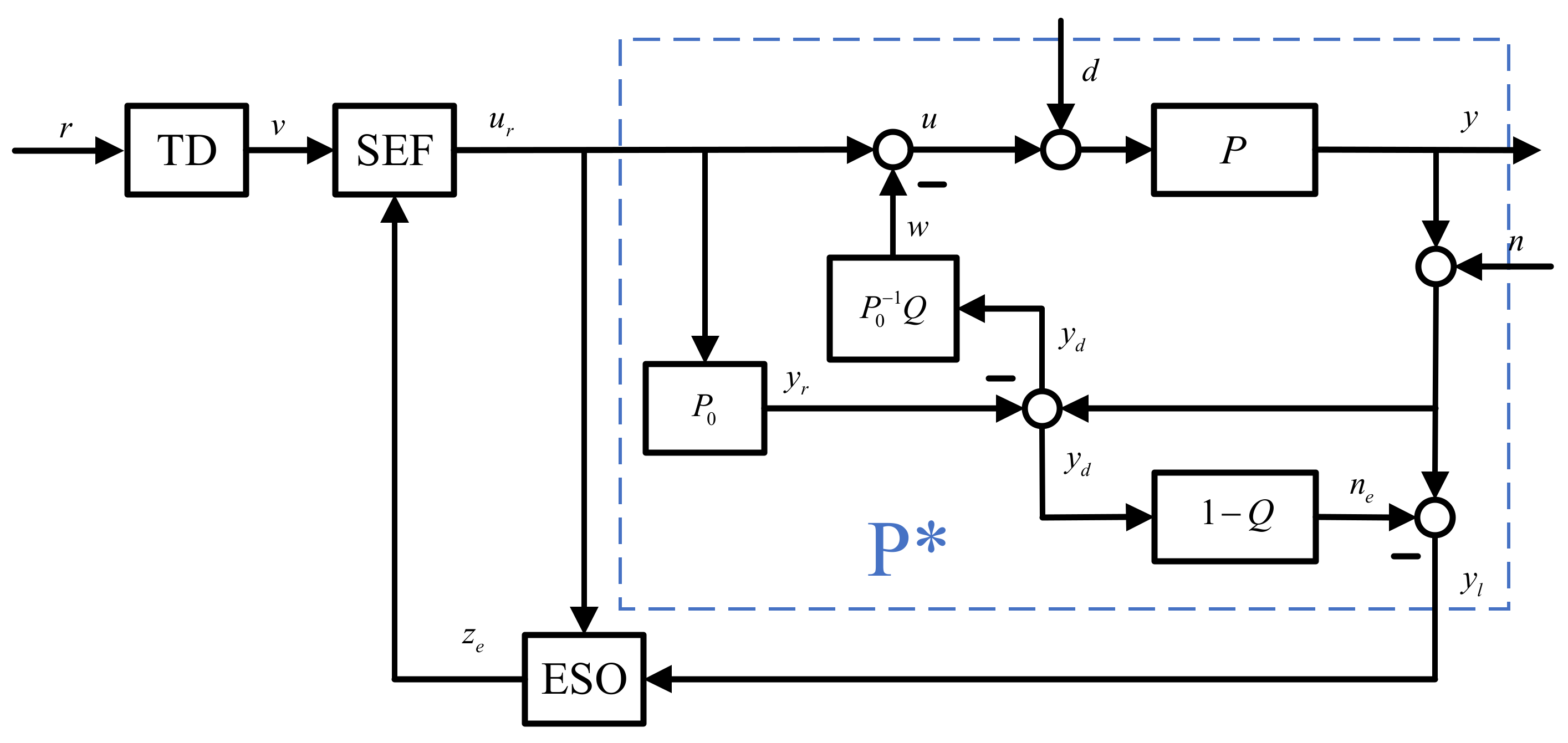
3. MNRDOB-Based ADRC
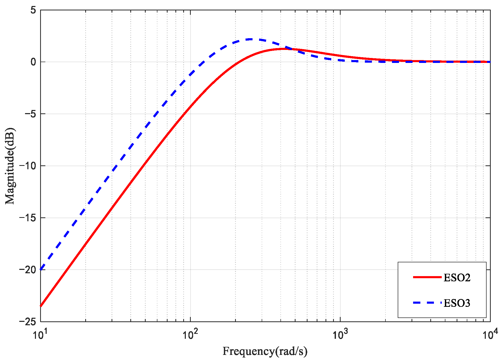
3.1. Modified Noise Reduction Disturbance Observer
3.2. Robust Stability Analysis
4. Simulation and Analysis
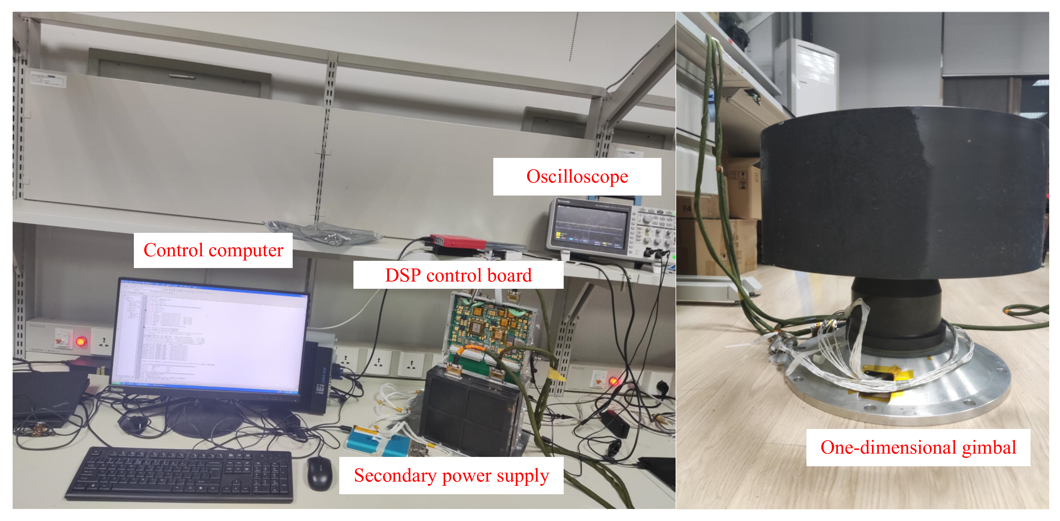
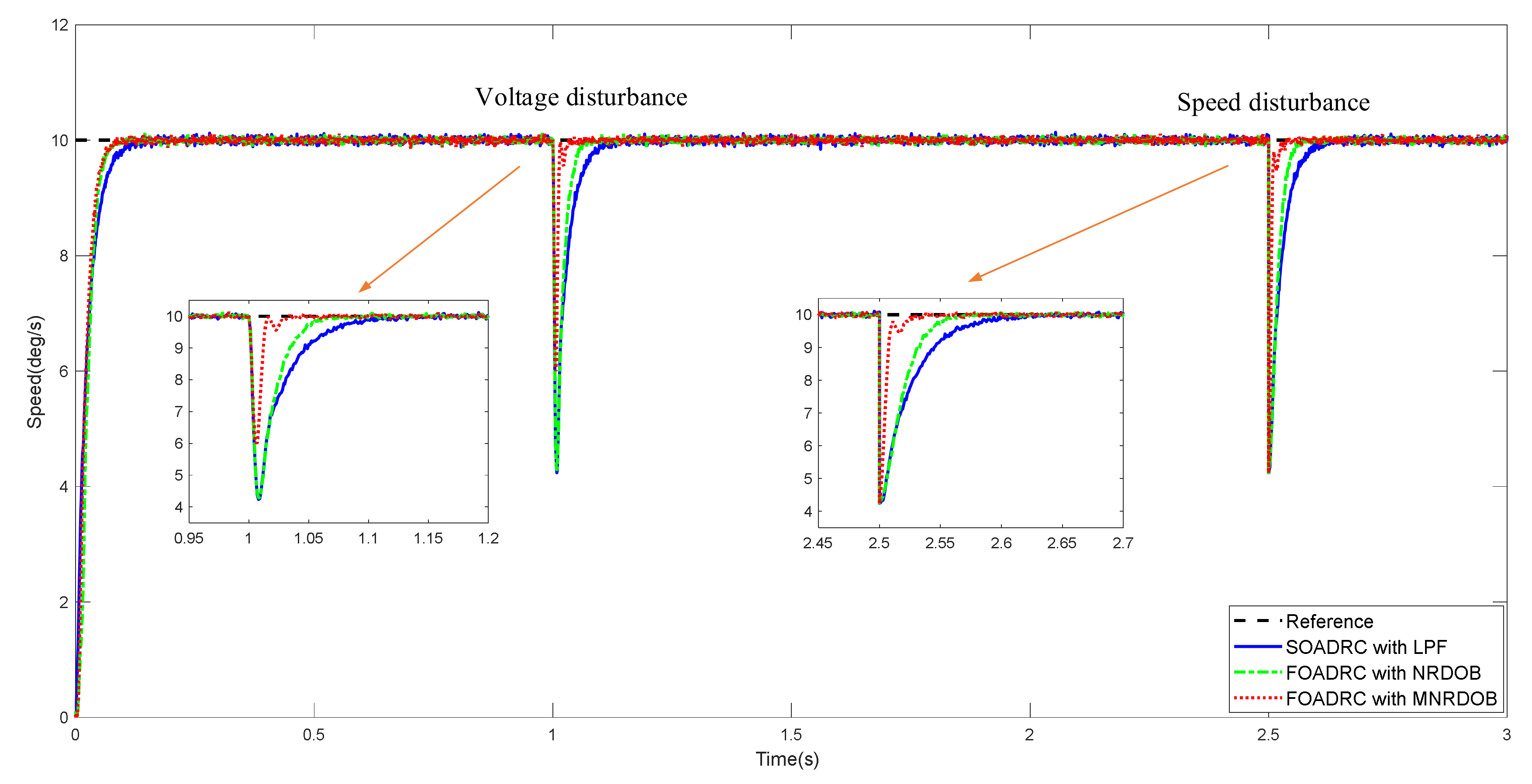
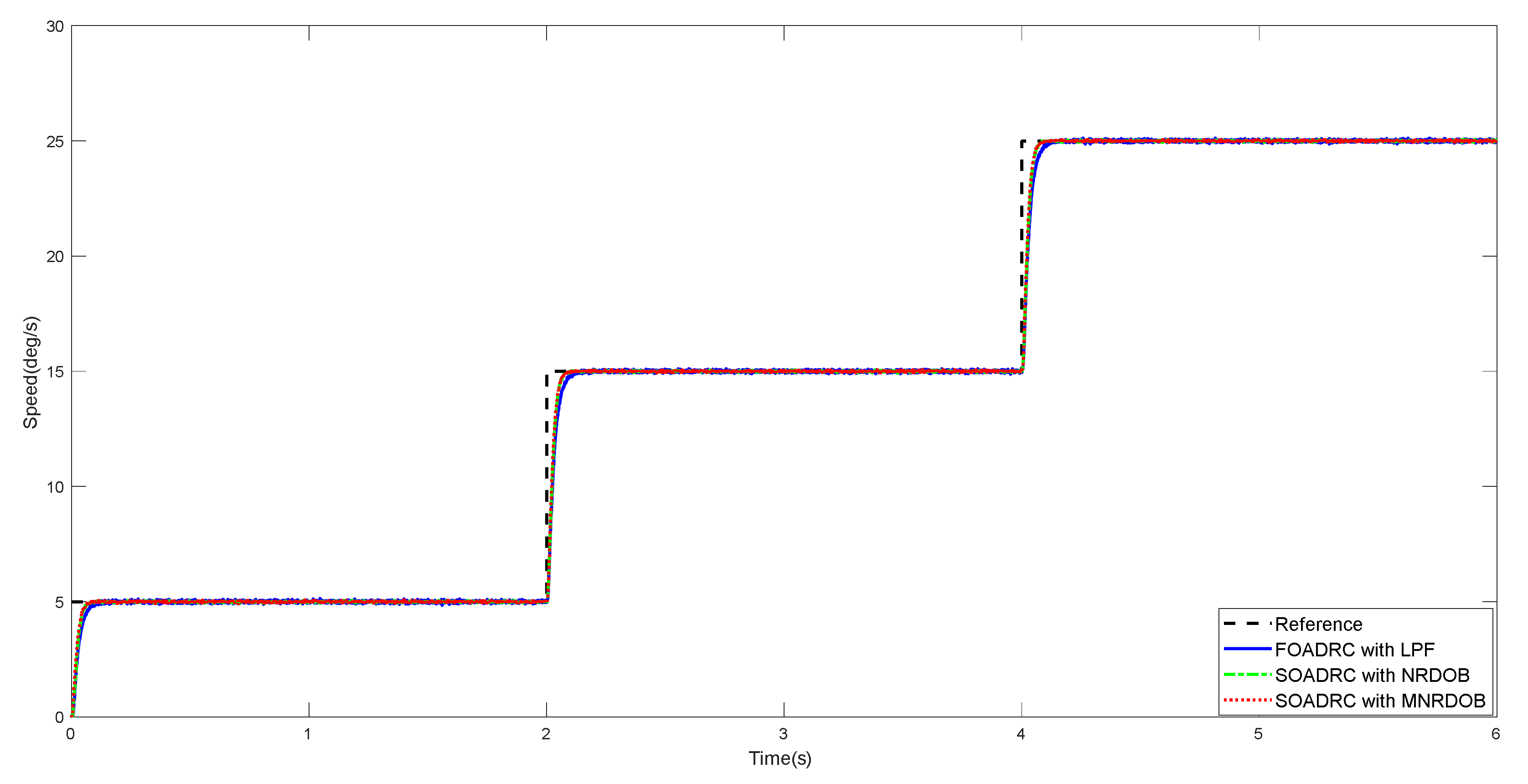
5. Experimental Results
6. Conclusions
Author Contributions
Funding
Acknowledgments
Conflicts of Interest
References
- Gao, Z. Active disturbance rejection control for nonlinear fractional-order systems. Int. J. Robust Nonlinear Control 2015, 26, 876–892. [Google Scholar] [CrossRef]
- Behzad, A.; Amin, N. Hardware Implementation of an ADRC Controller on a Gimbal Mechanism. IEEE Trans. Control Syst. Technol. 2018, 26, 2268–2275. [Google Scholar]
- Han, J. Active disturbance rejection controller and its applications. Control. Decis. 1998, 13, 19–23. (In Chinese) [Google Scholar]
- Han, J. From PID to Active Disturbance Rejection Control. IEEE Trans. Ind. Electron. 2009, 56, 900–906. [Google Scholar] [CrossRef]
- Gao, Z. Scaling and Bandwidth-Parameterization Based Controller Tuning. In Proceedings of the 2003 American Control Conference, Denver, CO, USA, 4–6 June 2003; pp. 4989–4996. [Google Scholar] [CrossRef]
- Yin, Z.; Du, C.; Liu, J.; Sun, X.; Zhong, Y. Research on Auto disturbance Rejection Control of Induction Motors Based on an Ant Colony Optimization Algorithm. IEEE Trans. Electron. 2018, 65, 3077–3094. [Google Scholar] [CrossRef]
- Qu, L.; Qiao, W.; Qu, L. Active-Disturbance-Rejection-Based Sliding-Mode Current Control for Permanent-Magnet Synchronous Motors. IEEE Trans. Power Electron. 2021, 36, 751–760. [Google Scholar] [CrossRef]
- Garrido, R.; Luna, L. Robust ultra-precision motion control of linear ultrasonic motors: A combined ADRC-Luenberger ob-server approach. Control Eng. Pract. 2021, 111, 104812. [Google Scholar] [CrossRef]
- Huang, Z.; Liu, Y.; Zheng, H.; Wang, S.; Ma, J.; Liu, Y. A self-searching optimal ADRC for the pitch angle control of an underwater thermal glider in the vertical plane motion. Ocean Eng. 2018, 159, 98–111. [Google Scholar] [CrossRef]
- Guo, T.; Song, D.; Li, K.; Li, C.; Yang, H. Pitch Angle Control with Model Compensation Based on Active Disturbance Rejection Controller for Underwater Gliders. J. Coast. Res. 2020, 36, 424. [Google Scholar] [CrossRef]
- Meng, Q.; Hou, Z. Active Disturbance Rejection Based Repetitive Learning Control with Applications in Power Inverters. IEEE Trans. Control. Syst. Technol. 2021, 29, 2038–2048. [Google Scholar] [CrossRef]
- Huang, D.; Min, Y.; Jian, Y.; Li, Y. Current-Cycle Iterative Learning Control for High-Precision Position Tracking of Piezo-electric Actuator System via Active Disturbance Rejection Control for Hysteresis Compensation. IEEE Trans. Ind. Electron. 2020, 67, 8680–8690. [Google Scholar] [CrossRef]
- Yue, M.; An, C.; Li, Z. Constrained Adaptive Robust Trajectory Tracking for WIP Vehicles Using Model Predictive Control and Extended State Observer. IEEE Trans. Syst. Man, Cybern. Syst. 2016, 48, 733–742. [Google Scholar] [CrossRef]
- Shyu, K.-K.; Lai, C.-K.; Tsai, Y.-W.; Yang, D.-I. A newly robust controller design for the position control of permanent-magnet synchronous motor. IEEE Trans. Ind. Electron. 2002, 49, 558–565. [Google Scholar] [CrossRef]
- Qi, L.; Shi, H. Adaptive position tracking control of permanent magnet synchronous motor based on RBF fast terminal sliding mode control. Neurocomputing 2013, 115, 23–30. [Google Scholar] [CrossRef]
- Sira-Ramírez, H.; Zurita-Bustamante, E. On the equivalence between ADRC and Flat Filter based controllers: A frequency domain approach. Control Eng. Pract. 2020, 107, 104656. [Google Scholar] [CrossRef]
- Ren, C.; Li, X.; Yang, X.; Ma, S. Extended State Observer-Based Sliding Mode Control of an Omnidirectional Mobile Robot With Friction Compensation. IEEE Trans. Ind. Electron. 2019, 66, 9480–9489. [Google Scholar] [CrossRef]
- Jo, N.H.; Jeon, C.; Shim, H. Noise Reduction Disturbance Observer for Disturbance Attenuation and Noise Suppression. IEEE Trans. Ind. Electron. 2016, 64, 1381–1391. [Google Scholar] [CrossRef]
- Wang, F.; Wang, R.; Liu, E.; Zhang, W. Stabilization Control Mothed for Two-Axis Inertially Stabilized Platform Based on Active Disturbance Rejection Control with Noise Reduction Disturbance Observer. IEEE Access 2019, 7, 99521–99529. [Google Scholar] [CrossRef]
- Zheng, Q.; Gaol, L.Q.; Gao, Z. On Stability Analysis of Active Disturbance Rejection Control for Nonlinear Time-Varying Plants with Unknown Dynamics. In Proceedings of the 2007 46th IEEE Conference on Decision and Control, New Orleans, LA, USA, 12–14 December 2007; pp. 3501–3506. [Google Scholar] [CrossRef]
- Ye, J.; Roy, S.; Godjevac, M.; Baldi, S. A Switching Control Perspective on the Offshore Construction Scenario of Heavy-Lift Ves-sels. IEEE Trans. Control Syst. Technol. 2021, 29, 470–477. [Google Scholar] [CrossRef]
- Roy, S.; Baldi, S.; Ioannou, P.A. An Adaptive Control Framework for Underactuated Switched Euler-Lagrange Systems. IEEE Trans. Autom. Control 2021, PP, 1. [Google Scholar] [CrossRef]
- Godbole, A.; Kolhe, J.; Talole, S. Performance Analysis of Generalized Extended State Observer in Tackling Sinusoidal Dis-turbances. IEEE Trans. Control Syst. Technol. 2013, 21, 2212–2223. [Google Scholar] [CrossRef]
- Moura, J.T.; Elmali, H.; Olgac, N. Sliding Mode Control with Sliding Perturbation Observer. J. Dyn. Syst. Meas. Control 1997, 119, 657–665. [Google Scholar] [CrossRef]
- Ohnishi, K.; Shibata, M.; Murakami, T. Motion control for advanced mechatronics. IEEE/ASME Trans. Mechatron. 1996, 1, 56–67. [Google Scholar] [CrossRef]
- Asignacion, A.; Haninger, K.; Oh, S.; Lee, H. High-Stiffness Control of Series Elastic Actuators Using a Noise Reduction Disturbance Observer. IEEE Trans. Ind. Electron. 2021, 69, 8212–8219. [Google Scholar] [CrossRef]
- Shim, H.; Jo, N.H. An almost necessary and sufficient condition for robust stability of closed-loop systems with disturbance observer. Automatica 2009, 45, 296–299. [Google Scholar] [CrossRef]
- Zhu, Q. Complete model-free siding mode control (CMFSMC). Sci. Rep. 2021, 111, 22565. [Google Scholar] [CrossRef] [PubMed]
- Nguyen, A.T.; Rafaq, M.S.; Choi, H.H.; Jung, J.-W. A Model Reference Adaptive Control Based Speed Controller for a Surface-Mounted Permanent Magnet Synchronous Motor Drive. IEEE Trans. Ind. Electron. 2018, 65, 9399–9409. [Google Scholar] [CrossRef]
- Zhang, Y.; Yin, Z.; Li, W.; Liu, J. Adaptive Sliding-Mode-Based Speed Control in Finite Control Set Model Predictive Torque Control for Induction Motors. IEEE Trans. Power Electron. 2020, 36, 8076–8087. [Google Scholar] [CrossRef]
- Alfehaid, A.A.; Strangas, E.G.; Khalil, H.K. Speed Control of Permanent Magnet Synchronous Motor With Uncertain Parameters and Unknown Disturbance. IEEE Trans. Control Syst. Technol. 2020, 29, 2639–2646. [Google Scholar] [CrossRef]
- Yang, Z.; Wang, D.; Sun, X.; Wu, J. Speed sensorless control of a bearingless induction motor with combined neural network and fractional sliding mode. Mechatronics 2021, 82, 102721. [Google Scholar] [CrossRef]
- Sami, I.; Ullah, S.; Basit, A.; Ullah, N.; Ro, J.-S. Integral Super Twisting Sliding Mode Based Sensorless Predictive Torque Control of Induction Motor. IEEE Access 2020, 8, 186740–186755. [Google Scholar] [CrossRef]


| Parameters | ||
|---|---|---|
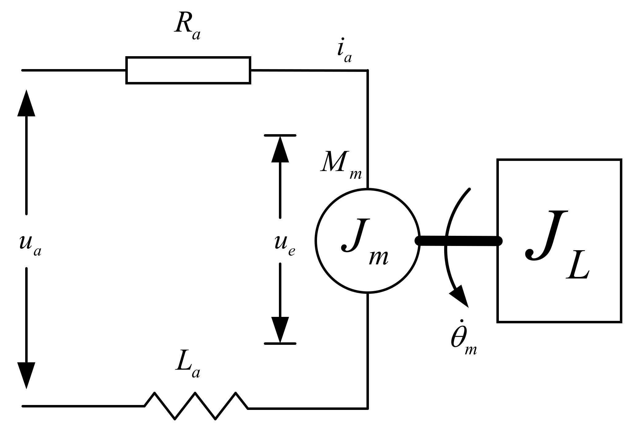
| Armature resistance | 2.25 (Ω) | |
| Armature inductance | 0.0067 (H) | |
| Total inertia | 0.011 (kg × m2) | |
| Back EMF coefficient | 2.67 (V/(rad/s)) | |
| Moment coefficient | 4.5 (N m/A) | |
| Viscous damping coefficient | 0.002 (N m/(rad/s)) | |
| Power amplification ratio | 5.4 |
| Control Methods | Noise in System Output (RMS/deg/s) | Noise in Control Input (RMS/V) |
|---|---|---|
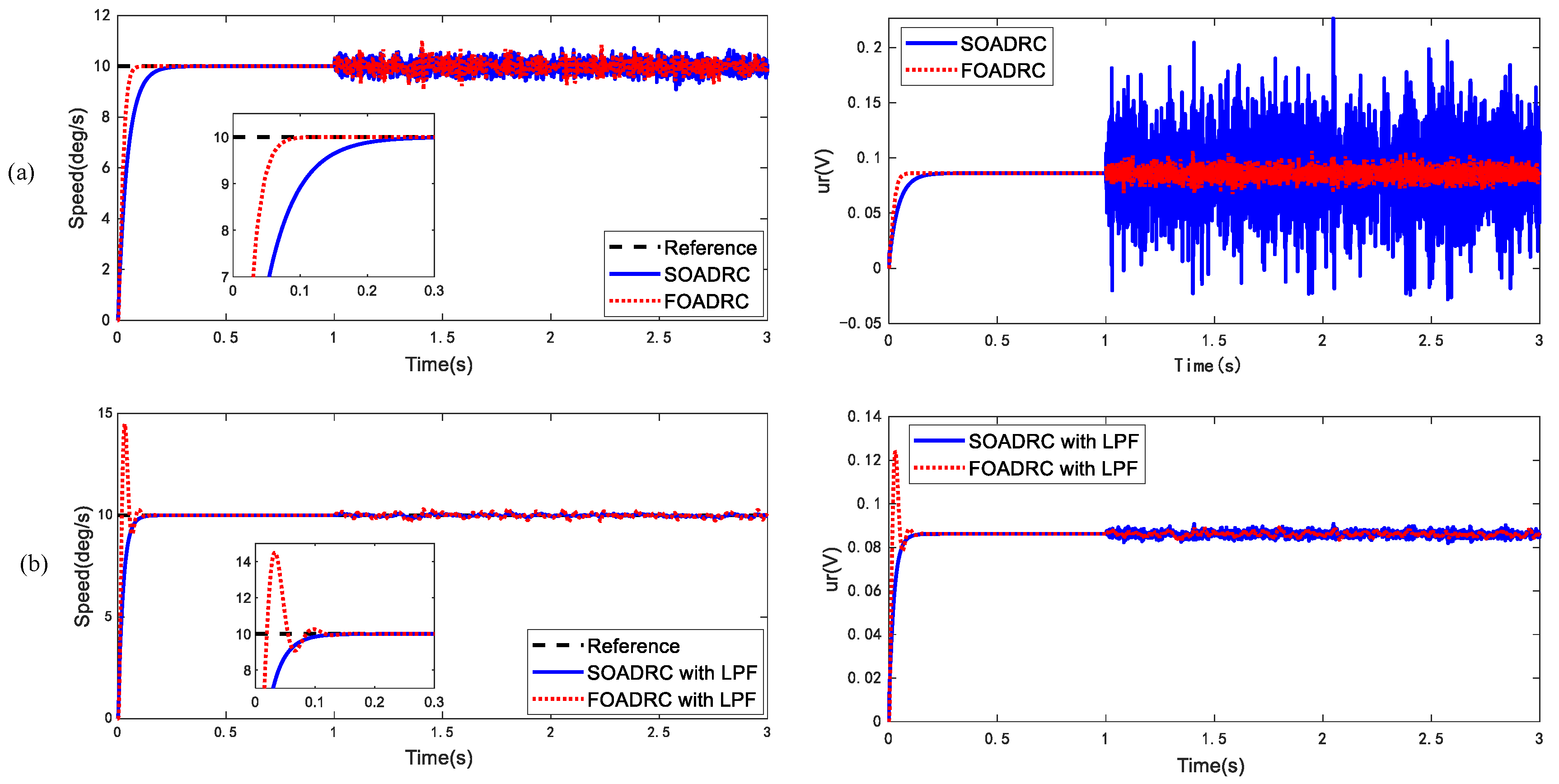
| SOADRC | 0.4079 | 0.0305 |
| SOADRC with LPF | 0.0577 | 0.0012 |
| FOADRC | 0.2298 | 0.0059 |
| FOADRC with LPF | 0.1654 | 0.0015 |
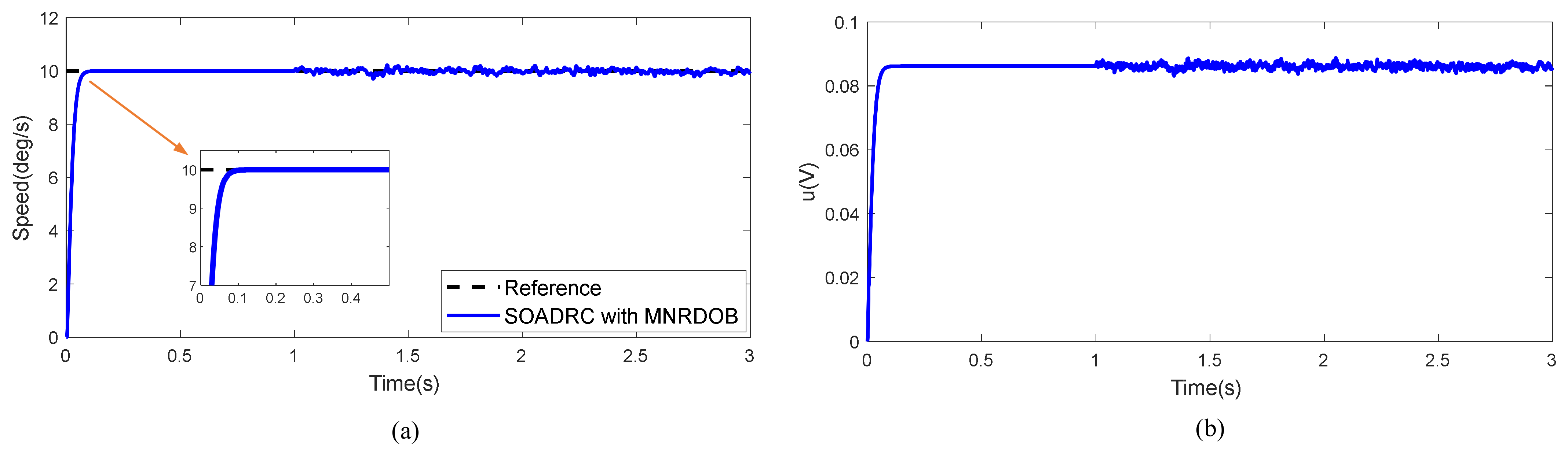
| FOADRC with MNRDOB | 0.0848 | 0.0008 |
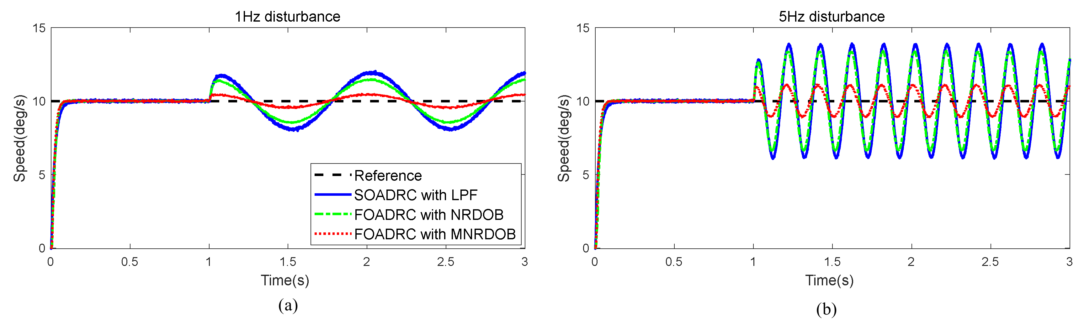
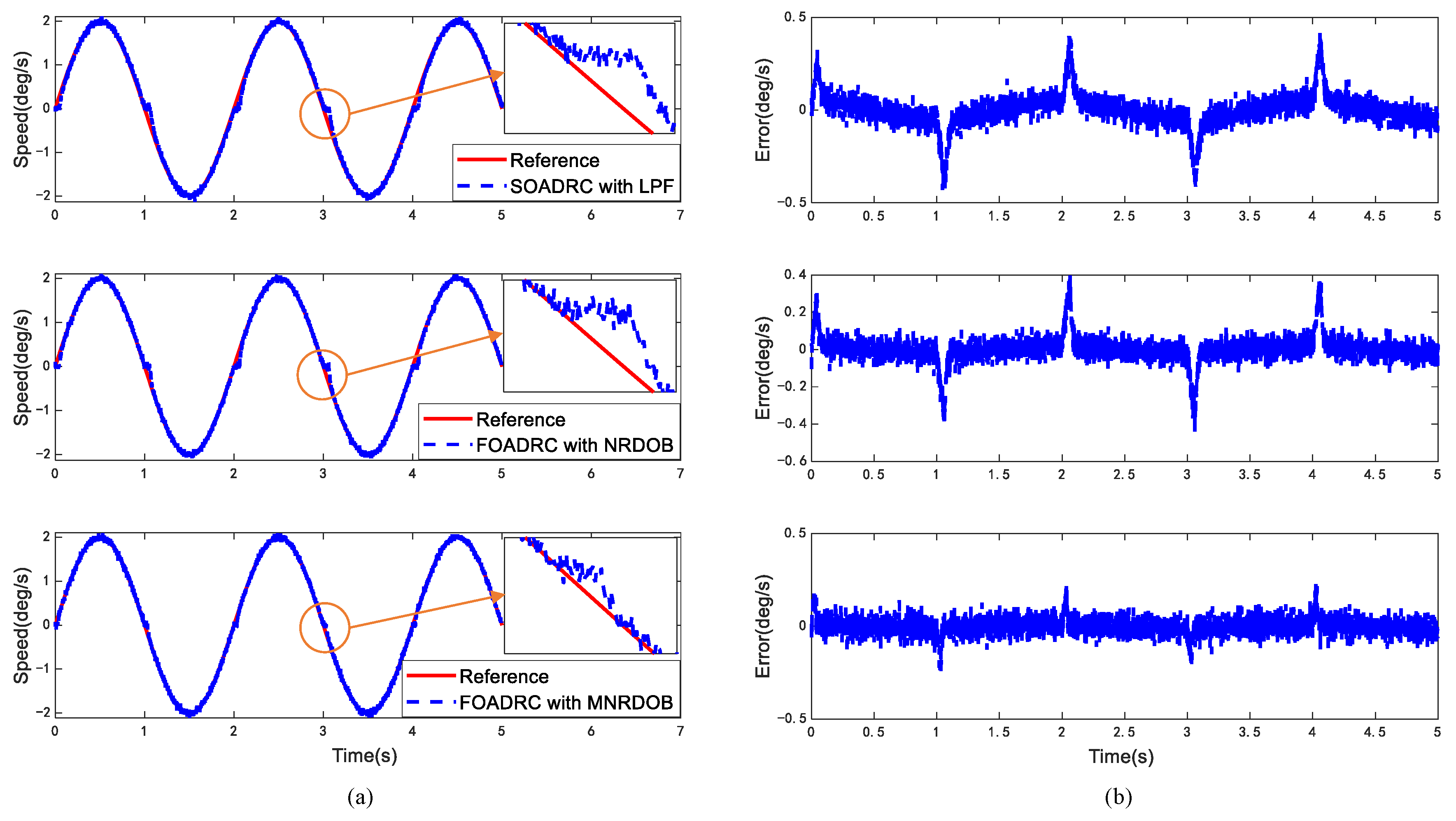
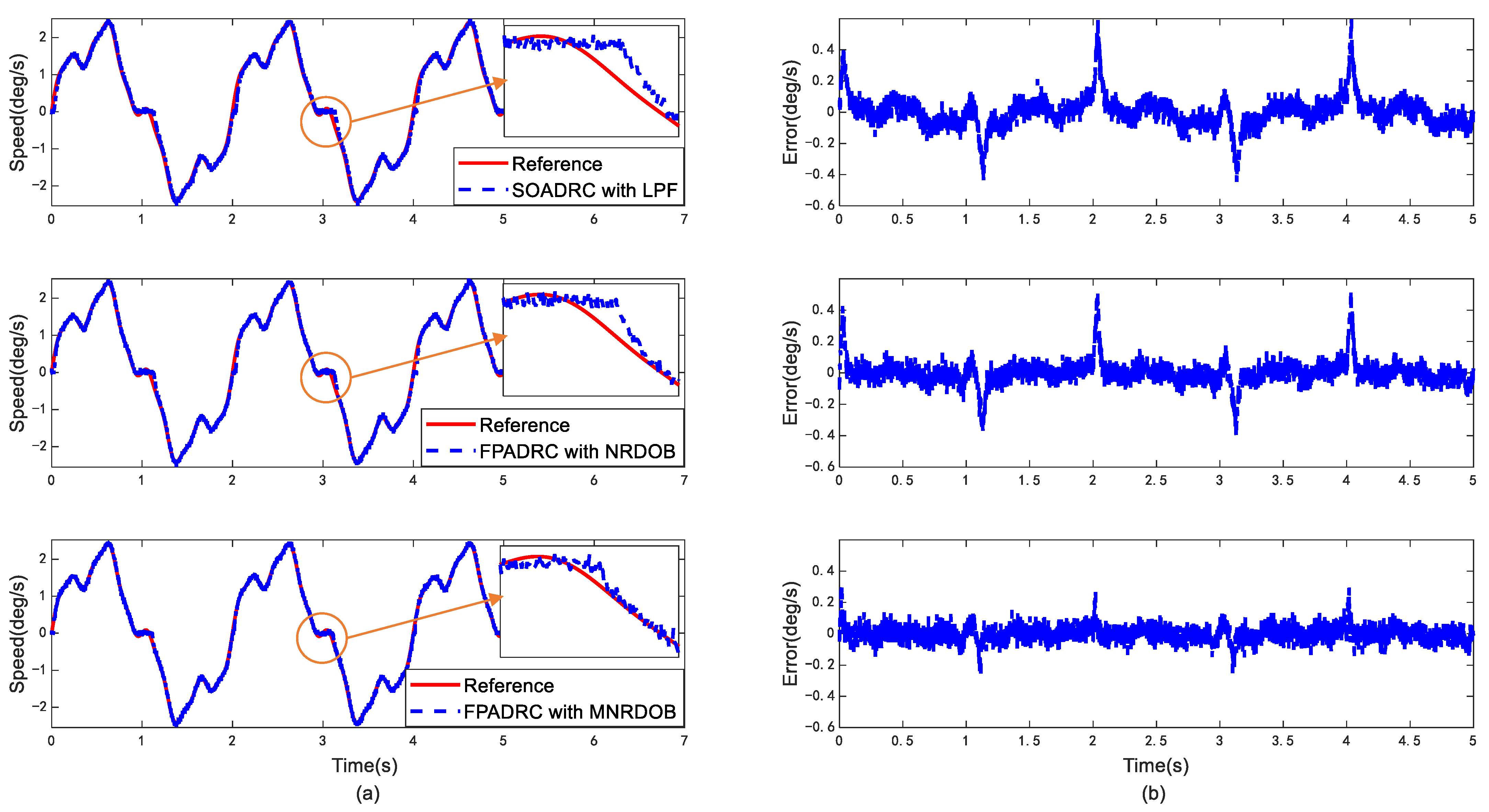
| Control Methods | Maximum Tracking Error (deg/s) | Tracking Error (deg/s) | ||||
|---|---|---|---|---|---|---|
| Sinusoidal Disturbance | Sine Signal | Mixed Signal | ||||
| 1 Hz | 5 Hz | Maximum | RMS | Maximum | RMS | |
| SOADRC with LPF | 2.021 | 3.914 | 0.416 | 0.0897 | 0.594 | 0.1043 |
| FOADRC with NRDOB | 1.537 | 3.462 | 0.397 | 0.0739 | 0.539 | 0.0865 |
| FOADRC with MNRDOB | 0.531 | 1.169 | 0.254 | 0.0485 | 0.292 | 0.0560 |
Publisher’s Note: MDPI stays neutral with regard to jurisdictional claims in published maps and institutional affiliations. |
© 2022 by the authors. Licensee MDPI, Basel, Switzerland. This article is an open access article distributed under the terms and conditions of the Creative Commons Attribution (CC BY) license (https://creativecommons.org/licenses/by/4.0/).
Share and Cite
Wang, F.; Liu, P.; Xie, M.; Jing, F.; Liu, B.; Cao, Y.; Ma, C. Robust Reduced-Order Active Disturbance Rejection Control Method: A Case Study on Speed Control of a One-Dimensional Gimbal. Machines 2022, 10, 592. https://doi.org/10.3390/machines10070592
Wang F, Liu P, Xie M, Jing F, Liu B, Cao Y, Ma C. Robust Reduced-Order Active Disturbance Rejection Control Method: A Case Study on Speed Control of a One-Dimensional Gimbal. Machines. 2022; 10(7):592. https://doi.org/10.3390/machines10070592
Chicago/Turabian StyleWang, Fan, Peng Liu, Meilin Xie, Feng Jing, Bo Liu, Yu Cao, and Caiwen Ma. 2022. "Robust Reduced-Order Active Disturbance Rejection Control Method: A Case Study on Speed Control of a One-Dimensional Gimbal" Machines 10, no. 7: 592. https://doi.org/10.3390/machines10070592