
Flatness-Based Active Disturbance Rejection Control for a PVTOL Aircraft System with an Inverted Pendular Load

 , , , , and
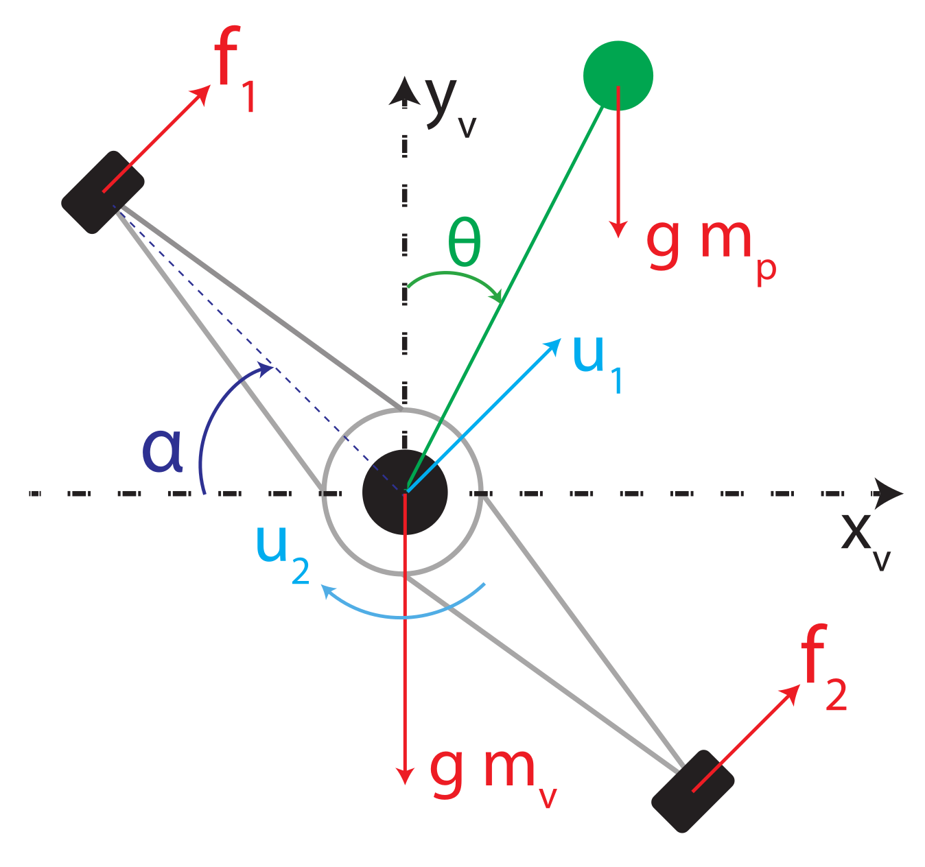
Abstract
:1. Introduction
- (i)
- a control strategy that uses the differential flatness property in the PVTOL aircraft system with an inverted pendular load in order to design a control for the height, roll attitude, horizontal position, and roll angle simultaneously, even in the presence of a crosswind;
- (ii)
- a control algorithm, which is robust against the presence of external disturbances and whose performance is competitive with respect to another robust controller of discontinuous nature; and
- (iii)
- a set of convenient transformations (cascade structure [3]), in which the linearized high-order system can be expressed as a various tandem lower-order systems depending on measurable variables that allow a controller formed by the combination of linear extended state observer-based ADRCs.
2. Mathematical Model
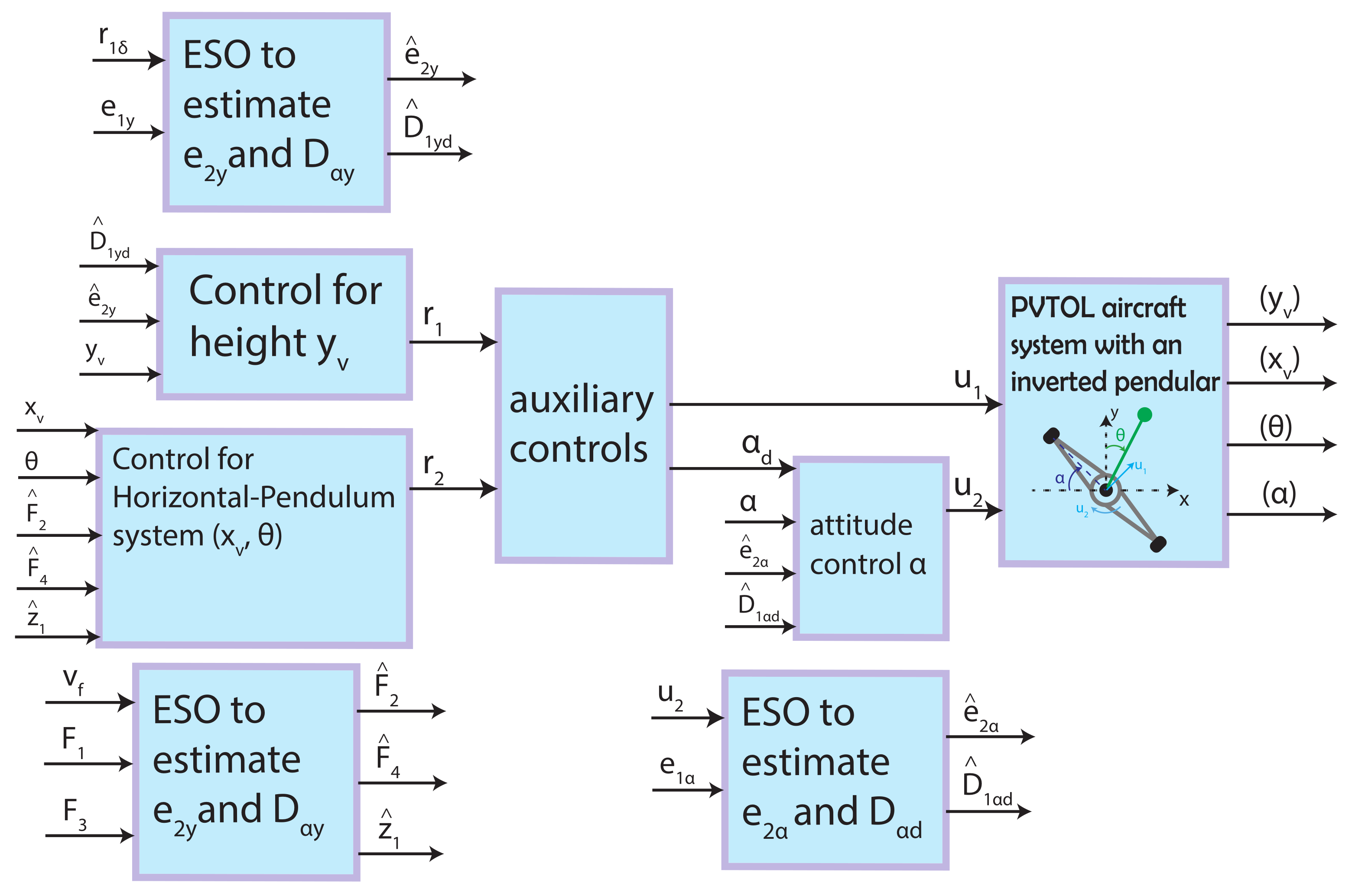
3. Control Scheme
3.1. Control for Angle
Linearized PVTOL Aircraft System with an Inverted Pendular Load
3.2. Height Control
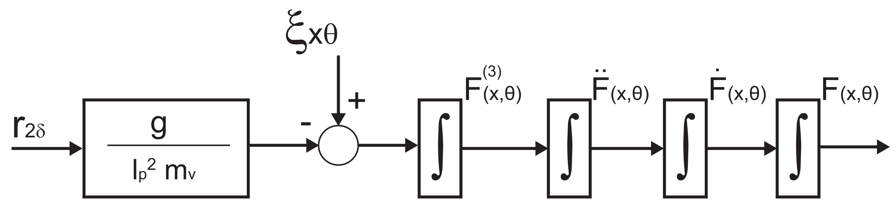
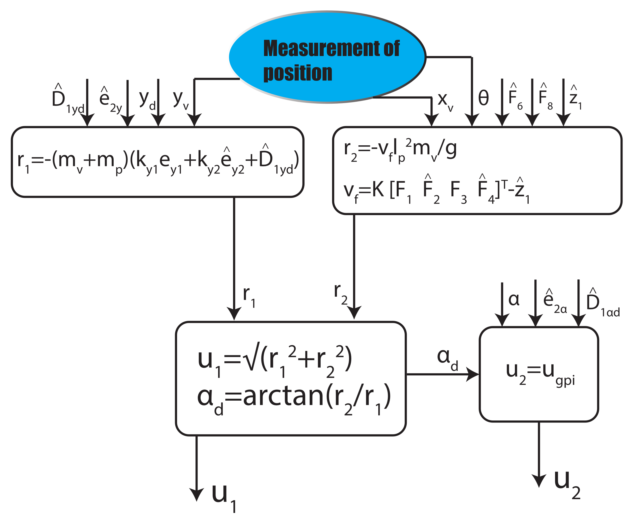
3.3. Control for Horizontal Displacement and Pendulum’s Angle
4. Numerical Simulations
5. Conclusions
Author Contributions
Funding
Institutional Review Board Statement
Informed Consent Statement
Data Availability Statement
Acknowledgments
Conflicts of Interest
Appendix A. Design of the Sliding Mode Control
Appendix A.1. Stability Proof for Height Dynamics
Appendix A.2. Stability Proof for (α,x v, θ) Dynamics
References
- Boubaker, O. The inverted pendulum: A fundamental benchmark in control theory and robotics. In Proceedings of the International Conference on Education and e-Learning Innovations, Sousse, Tunisia, 1–3 July 2012; pp. 1–6. [Google Scholar]
- Shkolnik, A.; Tedrake, R. High-dimensional underactuated motion planning via task space control. In Proceedings of the 2008 IEEE/RSJ International Conference on Intelligent Robots and Systems, Nice, France, 22–26 September 2008; pp. 3762–3768. [Google Scholar]
- Ramírez-Neria, M.; Sira-Ramírez, H.; Garrido-Moctezuma, R.; Luviano-Juarez, A. Linear active disturbance rejection control of underactuated systems: The case of the Furuta pendulum. ISA Trans. 2014, 53, 920–928. [Google Scholar] [CrossRef] [PubMed]
- Gómez-Estern, F.; Van der Schaft, A.J. Physical damping in IDA-PBC controlled underactuated mechanical systems. Eur. J. Control. 2004, 10, 451–468. [Google Scholar] [CrossRef] [Green Version]
- Jabbari Asl, H.; Oriolo, G.; Bolandi, H. Output feedback image-based visual servoing control of an underactuated unmanned aerial vehicle. Proc. Inst. Mech. Eng. Part I J. Syst. Control. Eng. 2014, 228, 435–448. [Google Scholar] [CrossRef]
- Rodríguez-Seda, E.J.; Tang, C.; Spong, M.W.; Stipanović, D.M. Trajectory tracking with collision avoidance for nonholonomic vehicles with acceleration constraints and limited sensing. Int. J. Robot. Res. 2014, 33, 1569–1592. [Google Scholar] [CrossRef]
- Ramirez-Neria, M.; Ochoa-Ortega, G.; Lozada-Castillo, N.; Trujano-Cabrera, M.A.; Campos-Lopez, J.P.; Luviano-Juárez, A. On the robust trajectory tracking task for flexible-joint robotic arm with unmodeled dynamics. IEEE Access 2016, 4, 7816–7827. [Google Scholar] [CrossRef]
- Furut, K.; Ochiai, T.; Ono, N. Attitude control of a triple inverted pendulum. Int. J. Control 1984, 39, 1351–1365. [Google Scholar] [CrossRef]
- Haddad, N.K.; Chemori, A.; Belghith, S. Robustness enhancement of IDA-PBC controller in stabilising the inertia wheel inverted pendulum: Theory and real-time experiments. Int. J. Control 2018, 91, 2657–2672. [Google Scholar] [CrossRef] [Green Version]
- Fantoni, I.; Lozano, R. Global stabilization of the cart-pendulum system using saturation functions. In Proceedings of the 42nd IEEE International Conference on Decision and Control (IEEE Cat. No. 03CH37475), Maui, HI, USA, 9–12 December 2003; Volume 5, pp. 4393–4398. [Google Scholar]
- Aguilar-Ibañez, C.; Suárez-Castañón, M.S.; Gutiérres-Frias, O.O. The direct Lyapunov method for the stabilisation of the Furuta pendulum. Int. J. Control 2010, 83, 2285–2293. [Google Scholar] [CrossRef]
- Moeini, A.; Lynch, A.F.; Zhao, Q. A backstepping disturbance observer control for multirotor UAVs: Theory and experiment. Int. J. Control 2021. [Google Scholar] [CrossRef]
- Hua, M.D.; Hamel, T.; Morin, P.; Samson, C. Introduction to feedback control of underactuated VTOLvehicles: A review of basic control design ideas and principles. IEEE Control. Syst. Mag. 2013, 33, 61–75. [Google Scholar]
- Liu, C.; Pan, J.; Chang, Y. PID and LQR trajectory tracking control for an unmanned quadrotor helicopter: Experimental studies. In Proceedings of the 2016 35th Chinese Control Conference (CCC), Chengdu, China, 27–29 July 2016; pp. 10845–10850. [Google Scholar]
- Xiong, L.; Yu, Z.; Wang, Y.; Yang, C.; Meng, Y. Vehicle dynamics control of four in-wheel motor drive electric vehicle using gain scheduling based on tyre cornering stiffness estimation. Veh. Syst. Dyn. 2012, 50, 831–846. [Google Scholar] [CrossRef]
- Lozano Hernández, Y.; Gutiérrez Frías, O.; Lozada-Castillo, N.; Luviano Juárez, A. Control algorithm for taking off and landing manoeuvres of quadrotors in open navigation environments. Int. J. Control. Autom. Syst. 2019, 17, 2331–2342. [Google Scholar] [CrossRef]
- Azinheira, J.R.; Moutinho, A. Hover control of an UAV with backstepping design including input saturations. IEEE Trans. Control. Syst. Technol. 2008, 16, 517–526. [Google Scholar] [CrossRef]
- Das, A.; Lewis, F.; Subbarao, K. Backstepping approach for controlling a quadrotor using lagrange form dynamics. J. Intell. Robot. Syst. 2009, 56, 127–151. [Google Scholar] [CrossRef]
- Zheng, E.H.; Xiong, J.J.; Luo, J.L. Second order sliding mode control for a quadrotor UAV. ISA Trans. 2014, 53, 1350–1356. [Google Scholar] [CrossRef] [PubMed]
- Hauser, J.; Sastry, S.; Meyer, G. Nonlinear control design for slightly non-minimum phase systems: Application to V/STOL aircraft. Automatica 1992, 28, 665–679. [Google Scholar] [CrossRef]
- Escobar, J.C.; Lozano, R.; Bonilla Estrada, M. PVTOL control using feedback linearisation with dynamic extension. Int. J. Control 2021, 94, 1794–1803. [Google Scholar] [CrossRef]
- Zavala-Rio, A.; Fantoni, I.; Lozano, R. Global stabilization of a PVTOL aircraft model with bounded inputs. Int. J. Control 2003, 76, 1833–1844. [Google Scholar] [CrossRef]
- López-Araujo, D.J.; Zavala-Río, A.; Fantoni, I.; Salazar, S.; Lozano, R. Global stabilisation of the PVTOL aircraft with lateral force coupling and bounded inputs. Int. J. Control 2010, 83, 1427–1441. [Google Scholar] [CrossRef]
- Aguilar-Ibanez, C.; Suarez-Castanon, M.S.; Meda-Campaña, J.; Gutierrez-Frias, O.; Merlo-Zapata, C.; Martinez-Castro, J.A. A simple approach to regulate a pvtol system using matching conditions. J. Intell. Robot. Syst. 2020, 98, 511–524. [Google Scholar] [CrossRef]
- Munoz, L.E.; Santos, O.; Castillo, P. Robust nonlinear real-time control strategy to stabilize a PVTOL aircraft in crosswind. In Proceedings of the 2010 IEEE/RSJ International Conference on Intelligent Robots and Systems, Taipei, Taiwan, 18–22 October 2010; pp. 1606–1611. [Google Scholar]
- Hehn, M.; D’Andrea, R. A flying inverted pendulum. In Proceedings of the 2011 IEEE International Conference on Robotics and Automation, Shangai, China, 9–13 May 2011; pp. 763–770. [Google Scholar]
- Krafes, S.; Chalh, Z.; Saka, A. Vision-based control of a flying spherical inverted pendulum. In Proceedings of the 2018 4th International Conference on Optimization and Applications (ICOA), Mohammedia, Morocco, 26–27 April 2018; pp. 1–6. [Google Scholar]
- Chen, H.; Yang, Y.; Sun, J. Improved Genetic Algorithm Based Optimal Control for A Flying Inverted Pendulum. In Proceedings of the 2019 3rd International Conference on Electronic Information Technology and Computer Engineering (EITCE), Xiamen, China, 18–20 October 2019; pp. 1428–1432. [Google Scholar]
- Nayak, A.; Banavar, R.N.; Maithripala, D. Stabilizing a spherical pendulum on a quadrotor. Asian J. Control 2020, 24, 1112–1121. [Google Scholar] [CrossRef]
- Aguilar-Ibanez, C.; Sira-Ramirez, H.; Suarez-Castanon, M.S.; Garrido, R. Robust trajectory-tracking control of a PVTOL under crosswind. Asian J. Control 2019, 21, 1293–1306. [Google Scholar] [CrossRef]
- Zhang, C.; Hu, H.; Gu, D.; Wang, J. Cascaded control for balancing an inverted pendulum on a flying quadrotor. Robotica 2017, 35, 1263–1279. [Google Scholar] [CrossRef] [Green Version]
- Ramírez-Neria, M.; Sira-Ramírez, H.; Garrido-Moctezuma, R.; Luviano-Juárez, A. Active disturbance rejection control of the inertia wheel pendulum through a tangent linearization approach. Int. J. Control. Autom. Syst. 2019, 17, 18–28. [Google Scholar] [CrossRef]
- Ramírez-Neria, M.; Sira-Ramírez, H.; Garrido-Moctezuma, R.; Luviano-Juárez, A. On the linear control of underactuated nonlinear systems via tangent flatness and active disturbance rejection control: The case of the ball and beam system. J. Dyn. Syst. Meas. Control 2016, 138, 104501. [Google Scholar] [CrossRef]
- Sira-Ramirez, H.; Agrawal, S.K. Differentially Flat systems; Crc Press: Boca Raton, FL, USA, 2018. [Google Scholar]
- Sira-Ramírez, H.; Luviano-Juárez, A.; Ramírez-Neria, M.; Zurita-Bustamante, E.W. Active Disturbance Rejection Control of Dynamic Systems: A Flatness Based Approach; Butterworth-Heinemann: Oxford, UK, 2018. [Google Scholar]
- Diop, S.; Fliess, M. Nonlinear observability, identifiability, and persistent trajectories. In Proceedings of the 30th IEEE Conference on Decision and Control, Brighton, UK, 11–13 December 1991; pp. 714–719. [Google Scholar]
- Ramírez-Neria, M.; Sira-Ramírez, H.; Garrido-Moctezuma, R.; Luviano-Juárez, A.; Gao, Z. Active Disturbance Rejection Control for Reference Trajectory Tracking Tasks in the Pendubot System. IEEE Access 2021, 9, 102663–102670. [Google Scholar] [CrossRef]


Publisher’s Note: MDPI stays neutral with regard to jurisdictional claims in published maps and institutional affiliations. |
© 2022 by the authors. Licensee MDPI, Basel, Switzerland. This article is an open access article distributed under the terms and conditions of the Creative Commons Attribution (CC BY) license (https://creativecommons.org/licenses/by/4.0/).
Share and Cite
Villaseñor Rios, C.A.; Luviano-Juárez, A.; Lozada-Castillo, N.B.; Carvajal-Gámez, B.E.; Mújica-Vargas, D.; Gutiérrez-Frías, O. Flatness-Based Active Disturbance Rejection Control for a PVTOL Aircraft System with an Inverted Pendular Load. Machines 2022, 10, 595. https://doi.org/10.3390/machines10070595
Villaseñor Rios CA, Luviano-Juárez A, Lozada-Castillo NB, Carvajal-Gámez BE, Mújica-Vargas D, Gutiérrez-Frías O. Flatness-Based Active Disturbance Rejection Control for a PVTOL Aircraft System with an Inverted Pendular Load. Machines. 2022; 10(7):595. https://doi.org/10.3390/machines10070595
Chicago/Turabian StyleVillaseñor Rios, Cesar Alejandro, Alberto Luviano-Juárez, Norma Beatriz Lozada-Castillo, Blanca Esther Carvajal-Gámez, Dante Mújica-Vargas, and Octavio Gutiérrez-Frías. 2022. "Flatness-Based Active Disturbance Rejection Control for a PVTOL Aircraft System with an Inverted Pendular Load" Machines 10, no. 7: 595. https://doi.org/10.3390/machines10070595