
Design Issues of Heavy Fuel APUs Derived from Automotive Turbochargers Part III: Combustor Design Improvement


Abstract
:1. Introduction
Summary of Previous Papers
2. Materials and Methods
2.1. Small Turbogas Issues
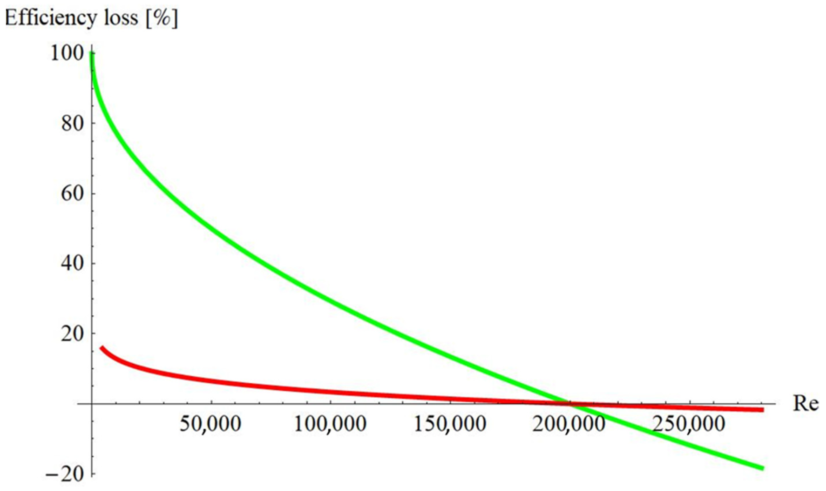
2.1.1. Small Axial Compressors Losses
2.1.2. Small Centrifugal Compressors Losses
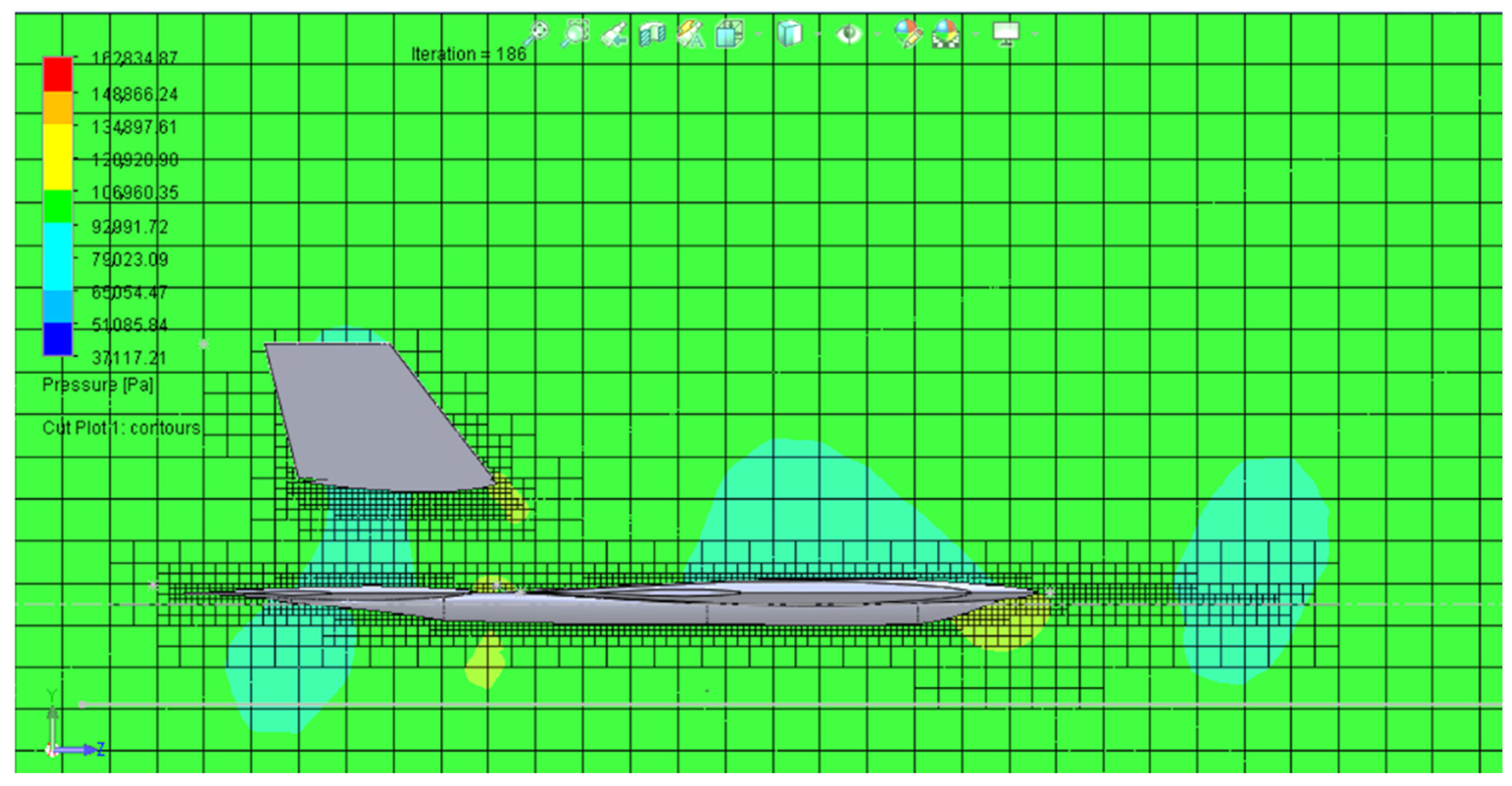
2.2. CFD Implementation
2.3. Reference Cycle of the Turbogas
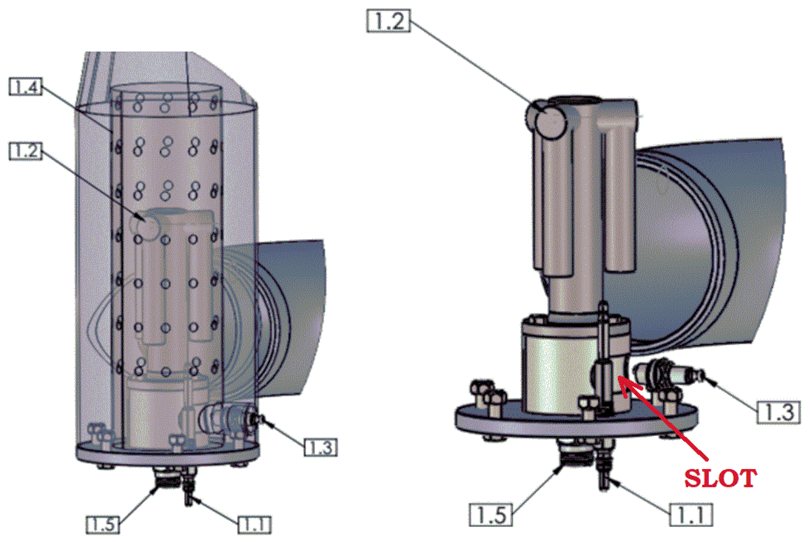
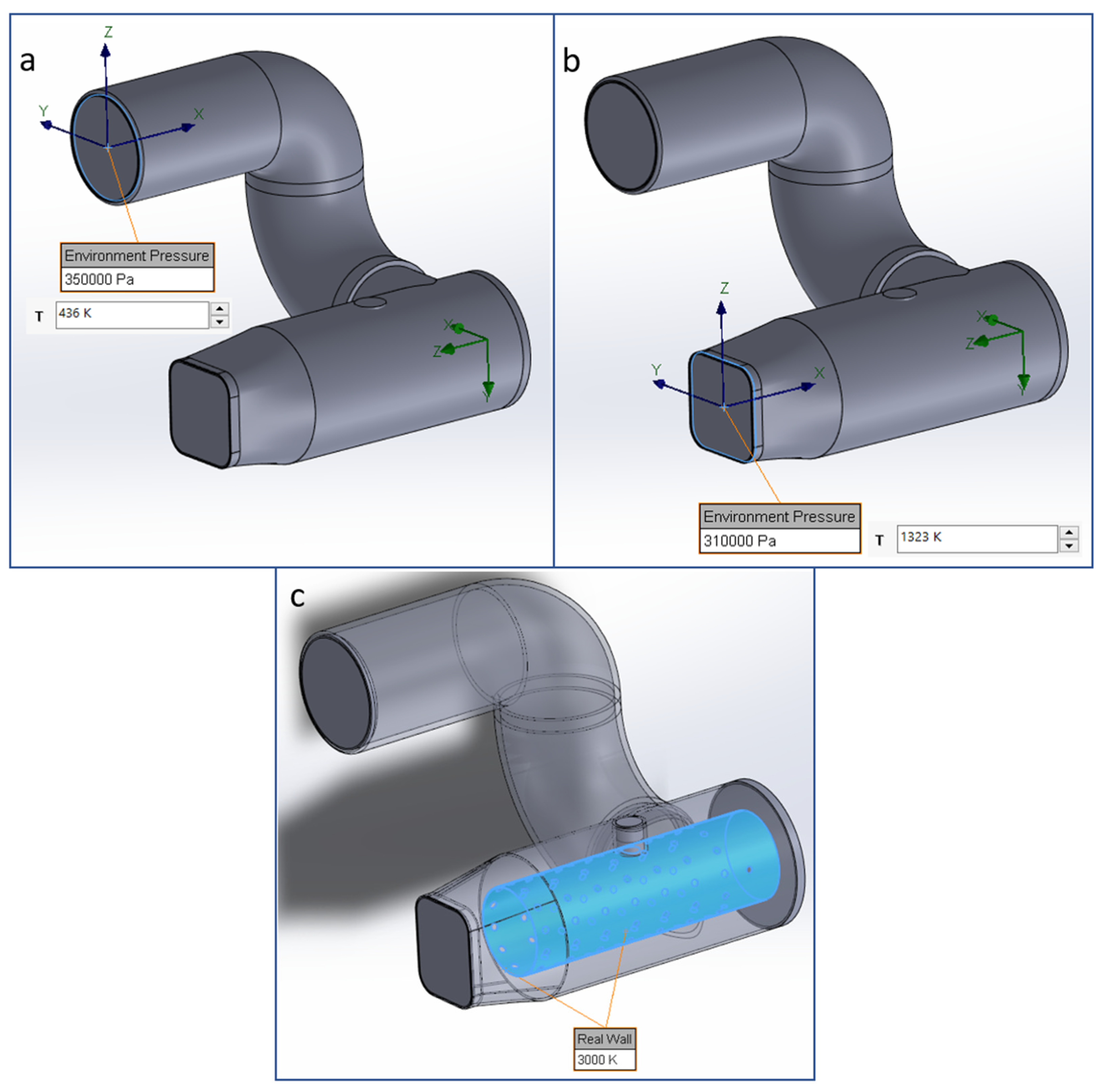
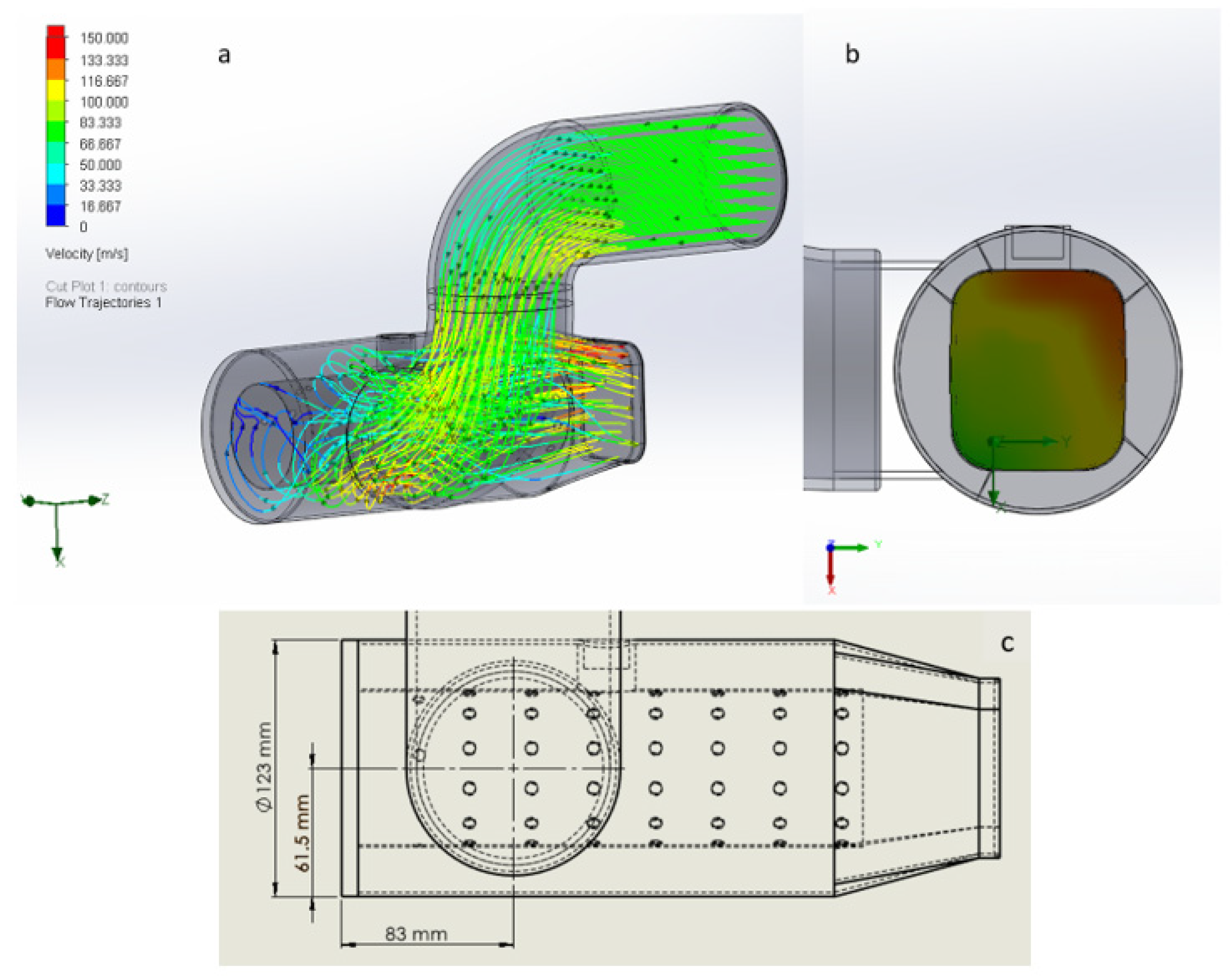
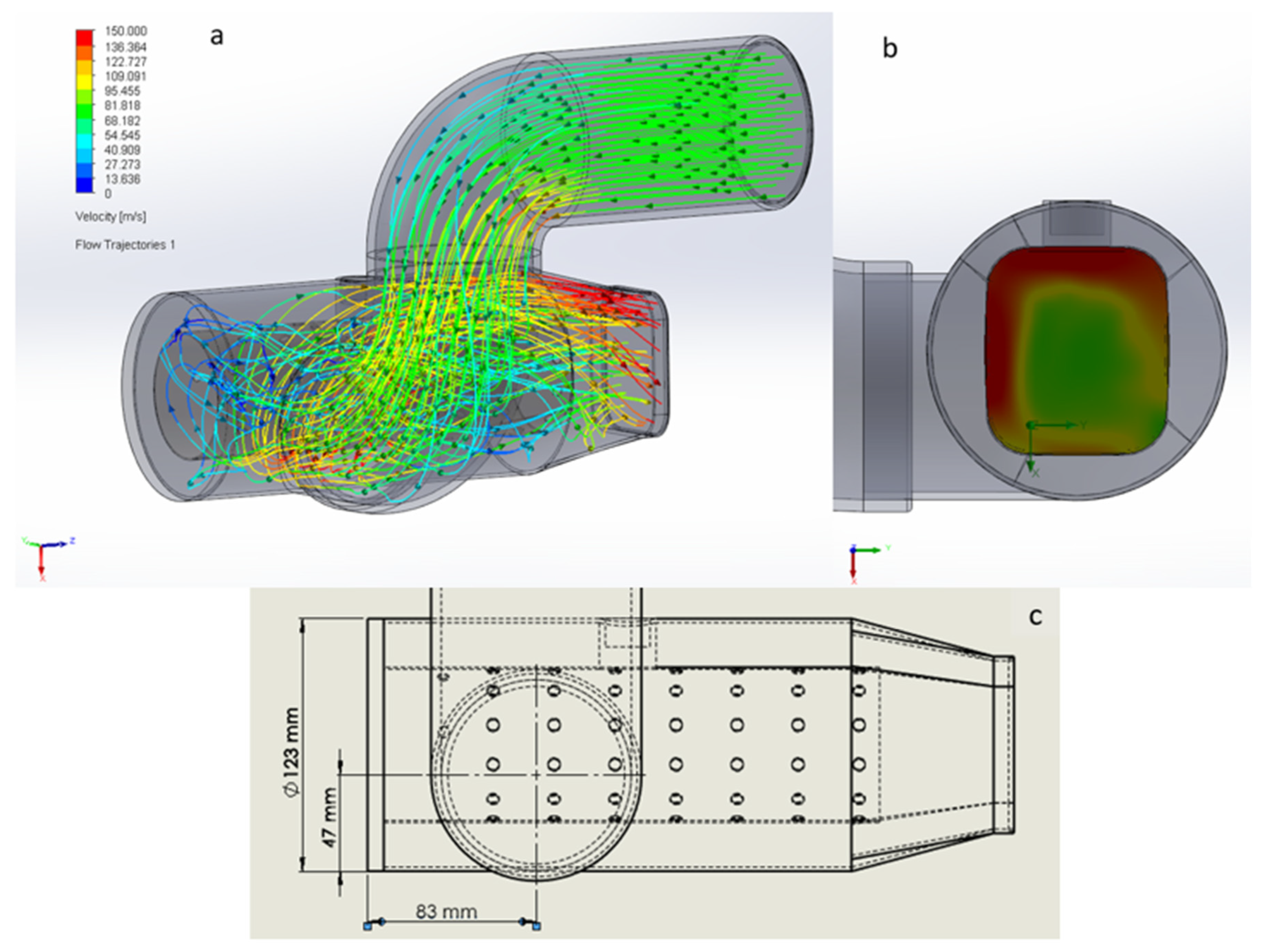
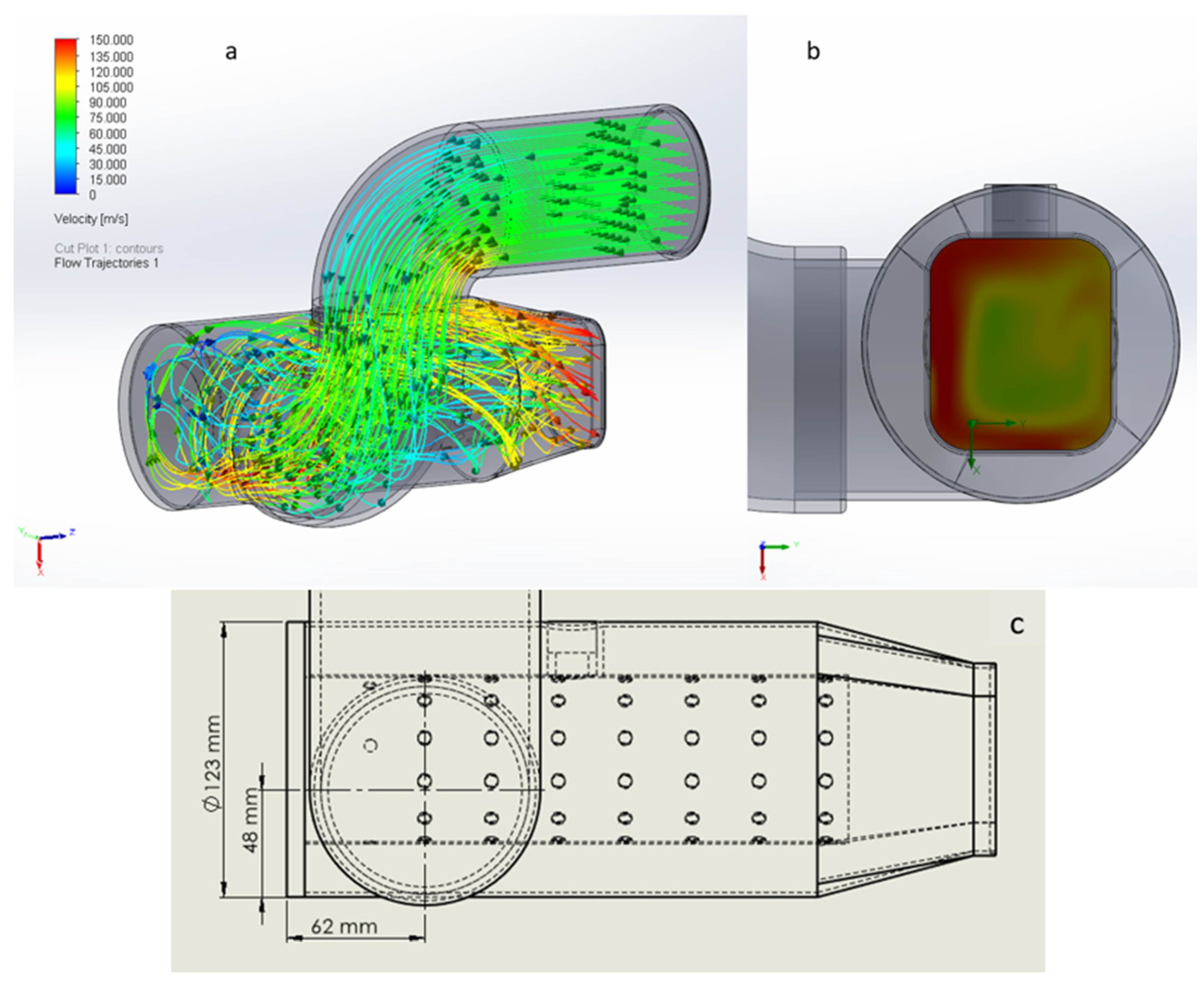
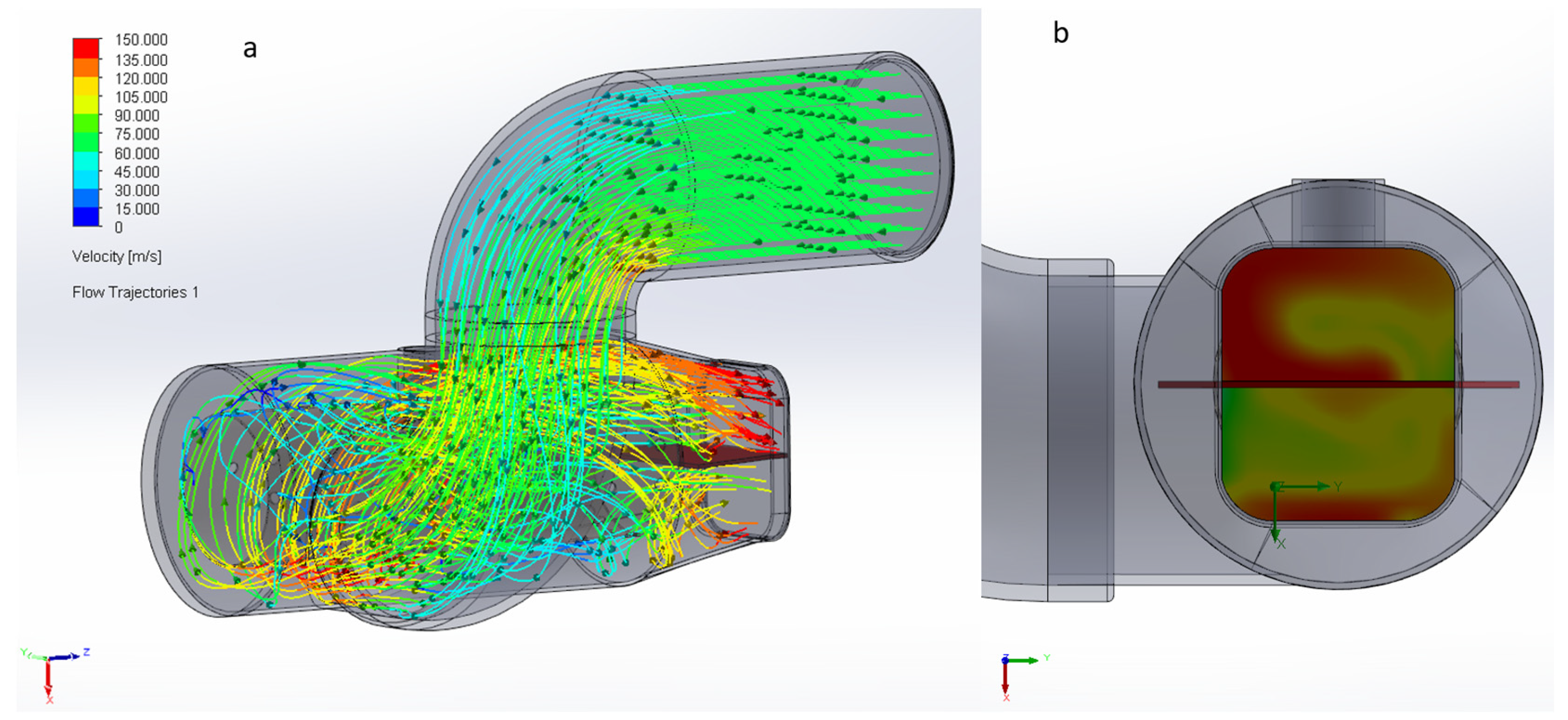
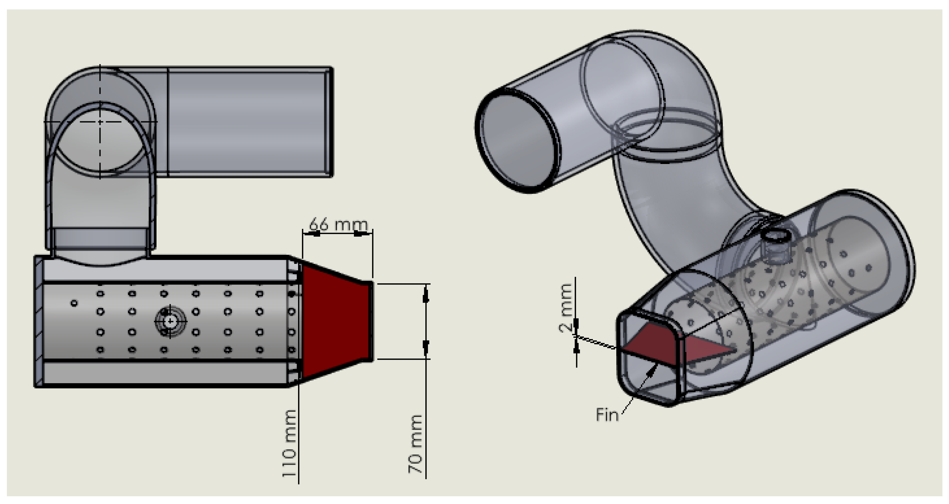
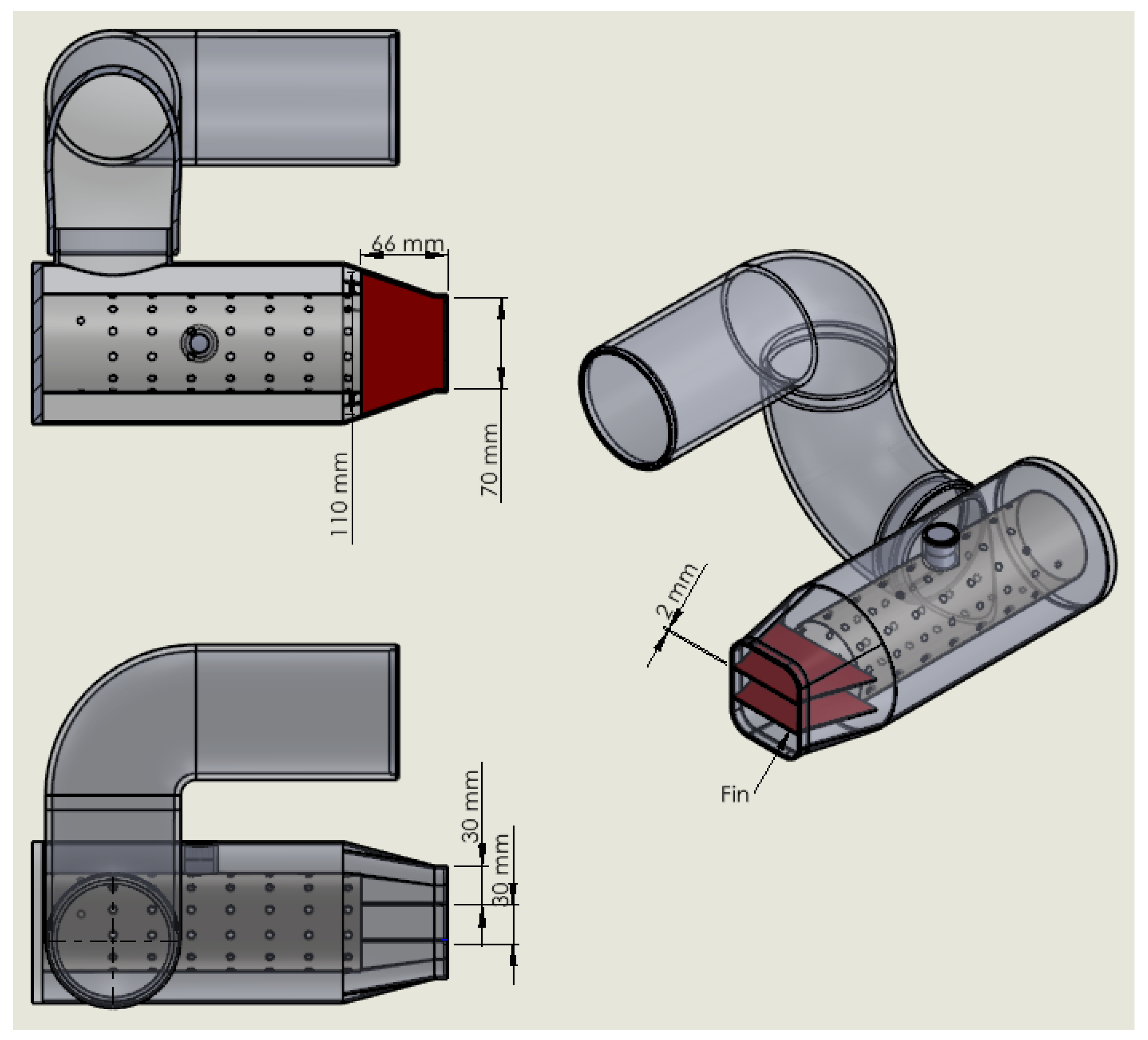
2.4. Improvement of Combustion Chamber Design
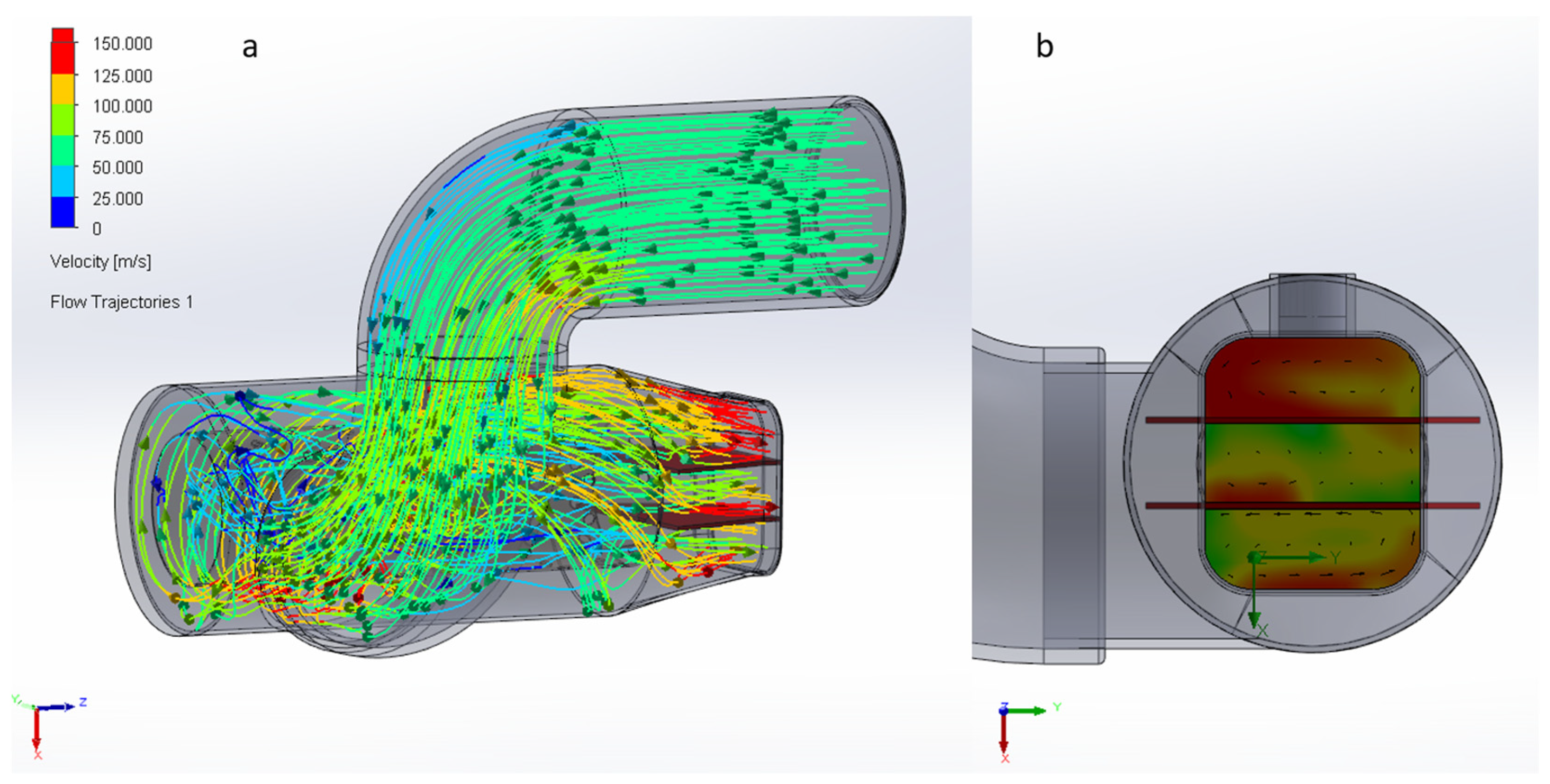
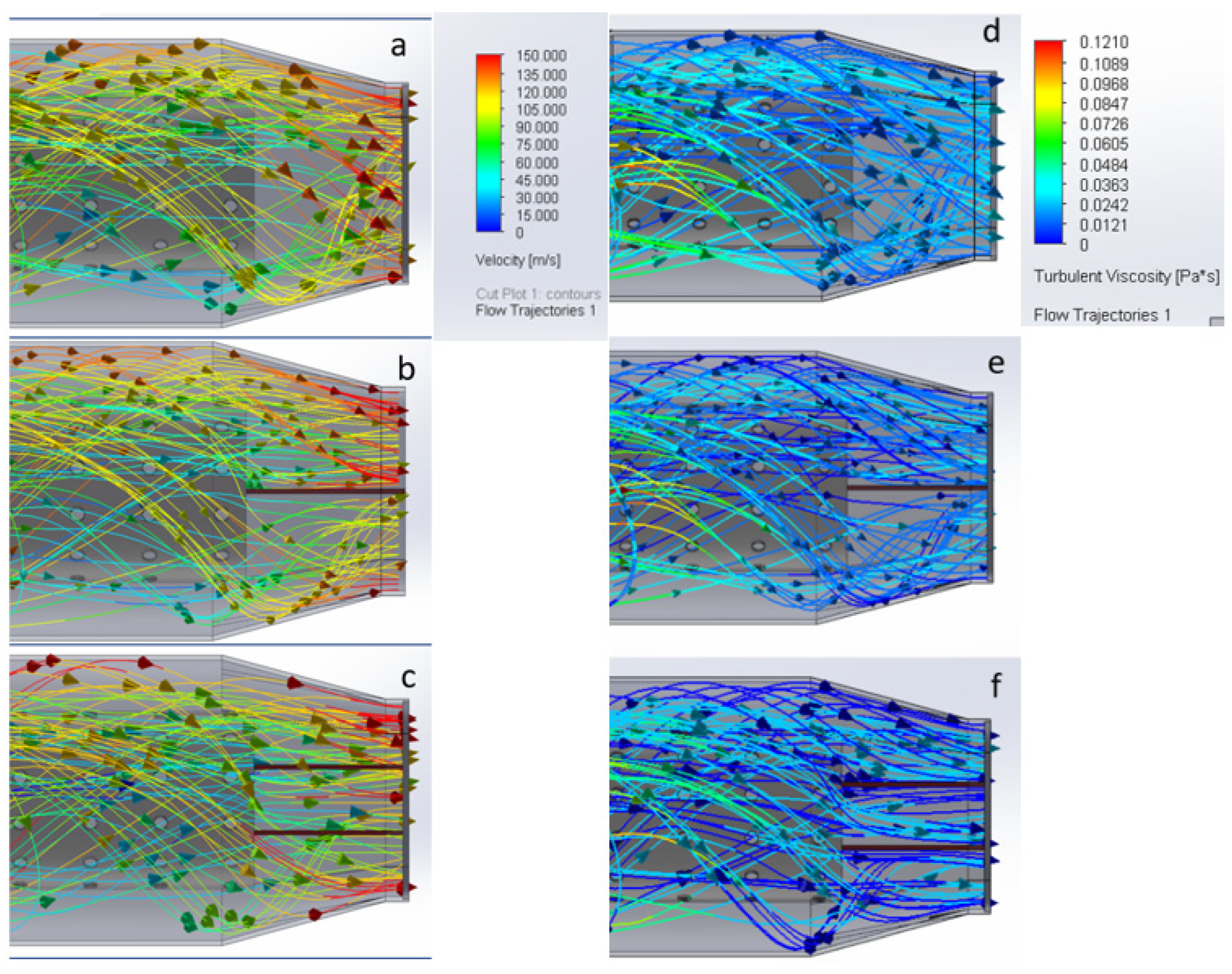
CFD Analysis with Distinctive Design Solutions
3. Results
4. Discussion
5. Conclusions
- The best configuration proved to be positioning the combustor intake at the bottom of the combustor to the most offset position from the combustor axis. A variation of the length of the combustor or the diameter has an extremely limited effect on the swirl motion and the turbine intake velocity pattern.
- Putting the combustion intake pipe at the bottom and the rearmost position helped increase the swirl motion of air inside the combustion chamber. However, additional solutions are required to reduce the outflow vortex.
- The insertion of fins at the turbine intake is proved to be beneficial in the case of making the airflow more stable and straighter. Additionally, due to the double fin solution, the design has straighter airflow.
- Overall values prove that there is not much pressure difference at turbine intake between the designs even if the outflow area slightly decreased because of fin parts.
- Further design solutions for this concept can be developed with the addition of enthalpy values of the combustion chamber by using equations and some additional boundary conditions in the simulation to analyze the thermal effects in this design.
Author Contributions
Funding
Institutional Review Board Statement
Informed Consent Statement
Data Availability Statement
Conflicts of Interest
References
- Piancastelli, L.; Ferretti, P.; Santi, G.M.; Scaltrini, A.; Cassani, S.; Calzini, F. Critical Design Issues of Heavy Fuel APUs Derived from Automotive Turbochargers. Part 1: Nominal Ambient Conditions. Technol. Ital. J. Eng. Sci. 2021, 65, 53–57. [Google Scholar] [CrossRef]
- Piancastelli, L.; Scaltrini, A.; Santi, G.M.; Risorgimento, V. Critical Design Issues of Heavy Fuel Turbogas Generators Derived from Automotive Turbochargers. Part II: The Improved Mach Method for off Design Performance Tuning. Technol. Ital. J. Eng. Sci. 2020, 64, 325–330. [Google Scholar] [CrossRef]
- Tiainen, J. Losses in Low-Reynolds-Number Centrifugal Compressors; LUT Yliopistopaino: Lappeenranta, Finland, 2018; ISBN 9789523352490. [Google Scholar]
- Piancastelli, L.; Gatti, A.; Frizziero, L.; Ragazzi, L.; Cremonini, M. CFD Analysis of the Zimmerman’s V173 Stol Aircraft. ARPN J. Eng. Appl. Sci. 2015, 10, 8063–8070. [Google Scholar]
- Frizziero, L.; Rocchi, I.; Donnici, G.; Pezzuti, E. Aircraft diesel engine turbocompound optimized. JP J. Heat Mass Transf. 2015, 11, 133–150. [Google Scholar] [CrossRef]
- Piancastelli, L.; Frizziero, L.; Bombardi, T. Bézier Based Shape Parameterization in High Speed Mandrel Design. Int. J. Heat Technol. 2014, 32, 57–63. [Google Scholar]
- Casey, M.; Robinson, C. A method to estimate the performance map of a centrifugal compressor stage. In Turbo Expo: Power for Land, Sea, and Air; ASME: New York, NY, USA, 2011; Volume 54679, pp. 1981–1993. [Google Scholar] [CrossRef]
- Xiao, G.; Yang, T.; Liu, H.; Ni, D.; Ferrari, M.L.; Li, M.; Luo, Z.; Cen, K.; Ni, M. Recuperators for Micro Gas Turbines: A Review. Appl. Energy 2017, 197, 83–99. [Google Scholar] [CrossRef]
- Ansaldo Energia AE-T100E Datasheet. 2017. Available online: https://www.ansaldoenergia.com/microturbines/Pages/Products.aspx (accessed on 4 July 2022).
- Ferretti, P.; Santi, G.M.; Leon-Cardenas, C.; Fusari, E.; Donnici, G.; Frizziero, L. Representative Volume Element (RVE) Analysis for Mechanical Characterization of Fused Deposition Modeled Components. Polymers 2021, 13, 3555. [Google Scholar] [CrossRef] [PubMed]
- Ferretti, P.; Santi, G.M.; Leon-Cardenas, C.; Freddi, M.; Donnici, G.; Frizziero, L.; Liverani, A. Molds with Advanced Materials for Carbon Fiber Manufacturing with 3D Printing Technology. Polymers 2021, 13, 3700. [Google Scholar] [CrossRef] [PubMed]
- Gavrilyuk, V.N.; Denisov, O.P.; Nakonechnyj, V.P.; Odintsov, E.V.; Sergienko, A.A.; Sobach, R. Numerical Simulation of Working Processes in Rocket Engine Combustion Chamber. In Proceedings of the Graz International Astronautical Federation Congress, Graz, Austria, 16–22 October 1993. [Google Scholar]
- Kalitzin, G.; Iaccarino, G. Turbulence Modeling in an Immersed-Boundary RANS Method. Cent. Turbul. Res. Annu. Res. Briefs 2002, 29, 415–426. [Google Scholar]
- Franke, R. Scattered Data Interpolation: Tests of Some Method. Math. Comput. 1982, 38, 181–200. [Google Scholar] [CrossRef]
- Ferziger, J.H.; Perić, M.; Street, R.L. Computational Methods for Fluid Dynamics; Springer: Berlin/Heidelberg, Germany, 2002; ISBN 3540420746. [Google Scholar]
- Van Driest, E.R. On Turbulent Flow near a Wall. J. Aeronaut. Sci. 1956, 23, 1007–1011. [Google Scholar] [CrossRef]
- Lam, C.K.G.; Bremhorst, K. A Modified Form of the K-ε Model for Predicting Wall Turbulence. J. Fluids Eng. 1981, 103, 456–460. [Google Scholar] [CrossRef]
- Wilcox, D.C. Turbulence Modeling for CFD, 3rd ed.; DCW Industries: Mumbai, India, 2006; Volume 2006. [Google Scholar]
- Silva, R.; Lacava, P. Preliminary Design of a Combustion Chamber for Microturbine Based in an Automotive Turbocharger. In Proceedings of the 22nd International Congress of Mechanical Engineering (COBEM 2013), Ribeirão Preto, Brazil, 3–7 November 2013. [Google Scholar]


| Symbol | Value | Unit |
|---|---|---|
| p1 (intake pressure) | 0.94 | bar |
| T1 (intake temperature) | 302.6 | K |
| p2 (pressure at compressor exit) | 3.32 | bar |
| T2 (temperature at compressor exit) | 457 | K |
| p3 (pressure at combustor exit) | 3.15 | bar |
| T3 (temperature at combustor exit) | 1323.15 | K |
| p4 (exhaust pressure) | 0.97 | bar |
| T4 (exhaust temperature) | 817.77 | K |
| m’(mass flow) | 1.21 | kg s−1 |
| P (output shaft power) | 141 | kW |
| Goal Name | Unit | Value | Averaged Value | Minimum Value | Maximum Value |
|---|---|---|---|---|---|
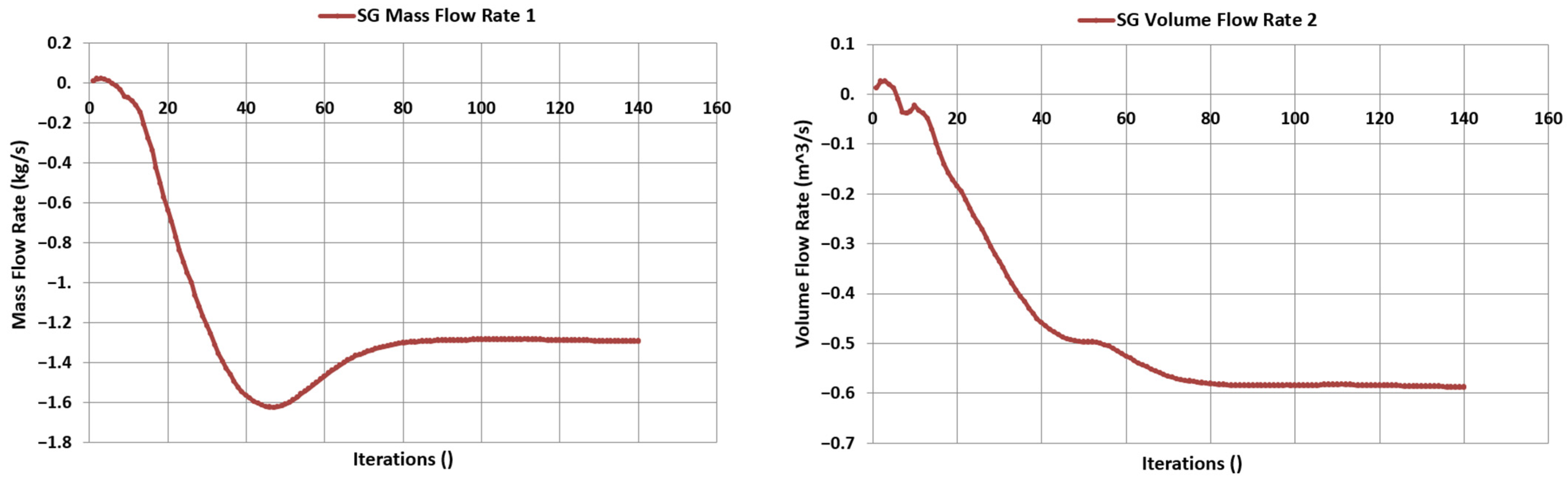
| SG Mass Flow Rate 1 | (kg/s) | −1.29894736 | −1.296344045 | −1.313922885 | −1.291387856 |
| SG Volume Flow Rate 2 | (m^3/s) | −0.59033924 | −0.588312778 | −0.590339241 | −0.587038829 |
| SG Average Velocity 3 | (m/s) | 119.0214988 | 119.2987803 | 118.831868 | 120.0288098 |
| SG Average Velocity (Z) 4 | (m/s) | 105.318486 | 104.9226897 | 104.6312092 | 105.318486 |
| SG Average Total Pressure 5 | (Pa) | 326610.8889 | 326729.0462 | 326577.5293 | 327025.5368 |
| Goal Name | Unit | Value | Averaged Value | Minimum Value | Maximum Value |
|---|---|---|---|---|---|
| SG Mass Flow Rate 1 | (kg/s) | −1.29093201 | −1.286113602 | −1.297684575 | −1.281673877 |
| SG Volume Flow Rate 2 | (m^3/s) | −0.58655097 | −0.58391615 | −0.58655097 | −0.58097484 |
| SG Average Velocity (Z) 3 | (m/s) | 107.341039 | 106.8365691 | 106.1400335 | 107.341039 |
| SG Average Velocity 4 | (m/s) | 119.1442447 | 119.1310012 | 118.670228 | 119.4863988 |
| SG Average Total Pressure 5 | (Pa) | 326678.4807 | 326692.9987 | 326592.1427 | 326884.9492 |
| Goal Name | Unit | Value | Averaged Value | Minimum Value | Maximum Value |
|---|---|---|---|---|---|
| SG Mass Flow Rate 1 | (kg/s) | −1.27298502 | −1.270702895 | −1.284514901 | −1.26641105 |
| SG Volume Flow Rate 2 | (m^3/s) | −0.57997544 | −0.578348927 | −0.579975437 | −0.57573282 |
| SG Average Velocity 3 | (m/s) | 116.6769594 | 116.4695425 | 115.9648319 | 116.6789374 |
| SG Average Velocity (Z) 4 | (m/s) | 108.969416 | 108.6195082 | 107.9705526 | 108.969416 |
| SG Average Total Pressure 5 | (Pa) | 325990.2905 | 325976.462 | 325882.7309 | 326185.7234 |
Publisher’s Note: MDPI stays neutral with regard to jurisdictional claims in published maps and institutional affiliations. |
© 2022 by the authors. Licensee MDPI, Basel, Switzerland. This article is an open access article distributed under the terms and conditions of the Creative Commons Attribution (CC BY) license (https://creativecommons.org/licenses/by/4.0/).
Share and Cite
Piancastelli, L.; Sali, M.; Leon-Cardenas, C. Design Issues of Heavy Fuel APUs Derived from Automotive Turbochargers Part III: Combustor Design Improvement. Machines 2022, 10, 583. https://doi.org/10.3390/machines10070583
Piancastelli L, Sali M, Leon-Cardenas C. Design Issues of Heavy Fuel APUs Derived from Automotive Turbochargers Part III: Combustor Design Improvement. Machines. 2022; 10(7):583. https://doi.org/10.3390/machines10070583
Chicago/Turabian StylePiancastelli, Luca, Merve Sali, and Christian Leon-Cardenas. 2022. "Design Issues of Heavy Fuel APUs Derived from Automotive Turbochargers Part III: Combustor Design Improvement" Machines 10, no. 7: 583. https://doi.org/10.3390/machines10070583