
An End-to-End Deep Learning Method for Dynamic Job Shop Scheduling Problem


Abstract
:1. Introduction
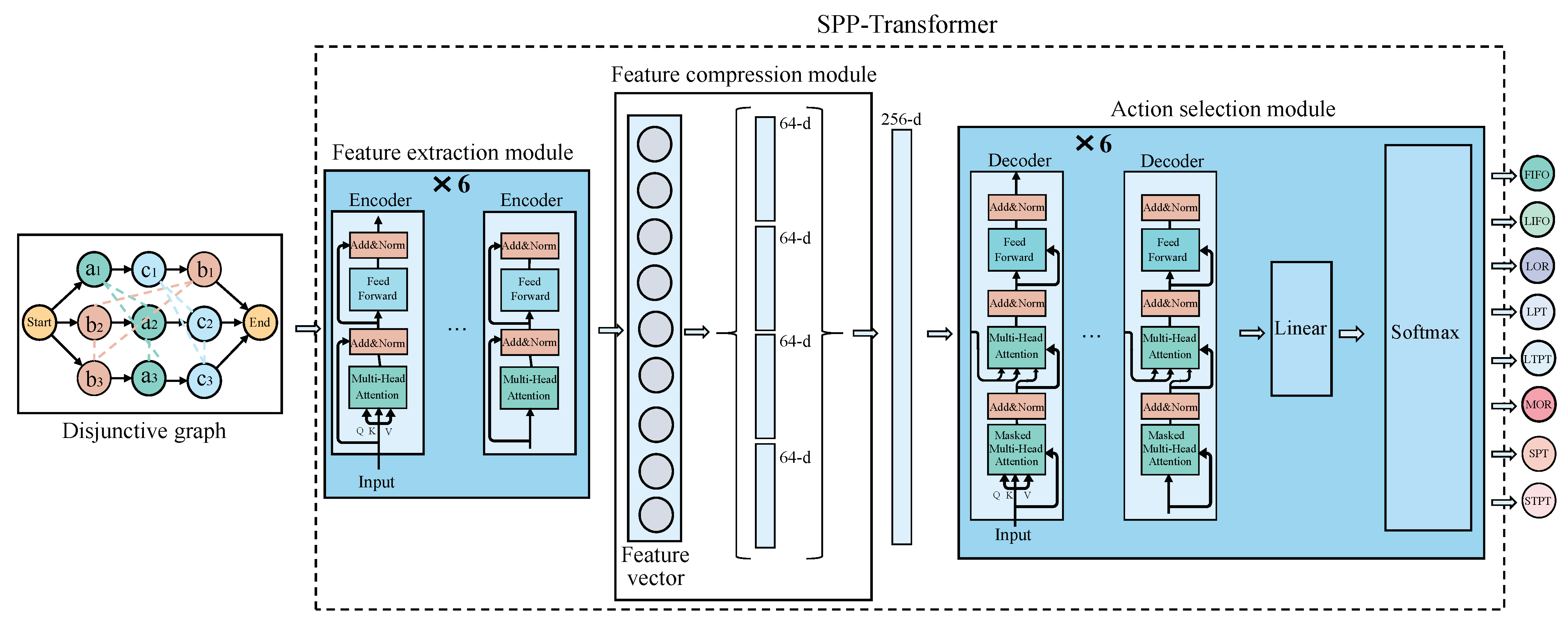
- An end-to-end transformer-based method is proposed, which takes the disjunctive graph as input and outputs the simple priority rule that can directly be applied in the production, providing a total data-driven method to solve DJSSP.
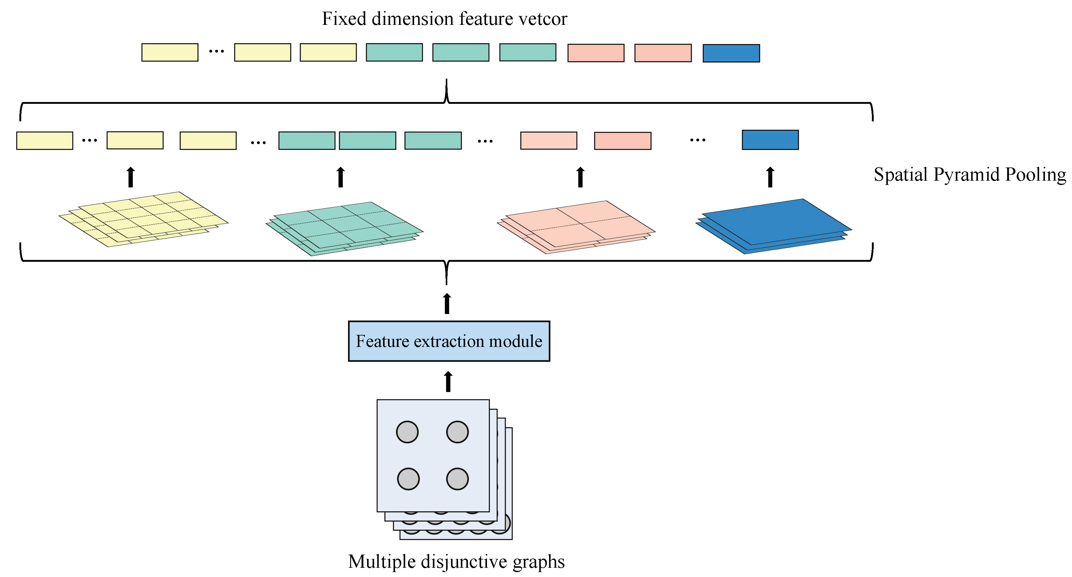
- A feature compression module that contains a spatial pyramid pooling (SPP) [33] layer is presented to enhance the generalizability of the proposed model. The feature compression module enables the proposed model to be applied to DJSSP instances of different sizes and be trained on the various-sized instances represented by the disjunctive graph. Thus, there is no need to train the model instance-by-instance.
- A sequence-to-action model that effectively deal with dynamic events is presented. Different from the conventional sequence-to-sequence deep learning models, the proposed sequence-to-action deep learning model reacts to the environment at each step according to the real-time states of the production environment. Thus, dynamic events that happen at an uncertain step can be well tackled without extra measures.
2. Materials and Methods
2.1. Problem Description
- (1)
- Each machine can only process one operation at the same time;
- (2)
- An operation is processed by only one machine at a time;
- (3)
- All jobs and machines are available at time 0;
- (4)
- An operation can not be interrupted if it has started unless machine breakdown;
- (5)
- The processing time of each operation may change during machining;
- (6)
- An operation cannot be processed until its preceding operations are completed.
2.2. Mathematical Model
3. Proposed Method
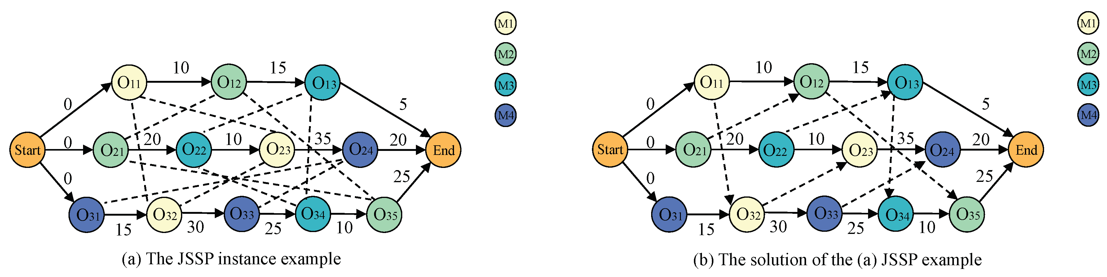
3.1. Input and Output Representation
3.1.1. Input Representation
- (1)
- Operation identified number: The corresponding serial number of this operation in the job is added to the vertex;
- (2)
- Job identified number: If a job includes the operation, its serial number is added to the vertex;
- (3)
- Machine identified number: If a machine can process this operation, its serial number is added to the vertex. And 0 is added if there are no machines that can process this operation;
- (4)
- Node situation: 1, 0, and −1 represent that the operation is finished, being processed, and unfinished, respectively;
- (5)
- Completion rate: When this operation is finished, the completion rate of the entire job;
- (6)
- Number of subsequent operations: The number of remaining operations to be finished;
- (7)
- Time for waiting: The amount of time that has elapsed since the start before this operation can be processed;
- (8)
- Processing time: The time required to process the operation;
- (9)
- Remaining time: The remaining processing time of the operation (0 for unprocessed);
- (10)
- Doable: It is “True” if the operation is doable.
3.1.2. Output Representation
- (1)
- First In First Out (FIFO): The machine will first process the job that first arrived at the queue of the machine;
- (2)
- Last In Last Out (LIFO): The machine will first process the job that last arrived at the queue of the machine;
- (3)
- Most Operations Remaining (MOR): The machine will first process the job that has the most remaining operations;
- (4)
- Least Operations Remaining (LOR): The machine will first process the job that has the least remaining operations;
- (5)
- Longest Processing Time (LPT): The machine will first process the job that has the longest processing time;
- (6)
- Shortest Processing Time (SPT): The machine will first process the job that has the shortest processing time;
- (7)
- Longest Total Processing Time (LTPT): The machine will first process the job that has the longest total processing time;
- (8)
- Shortest Total Processing Time (STPT): The machine will first process the job that has the shortest total processing time.
3.2. Transformer Layer
3.2.1. Feature Extraction Module
3.2.2. Feature Compression Module
3.2.3. Action Selection Module
3.3. Training Procedure
4. Numerical Experiments
4.1. Experimental Setup
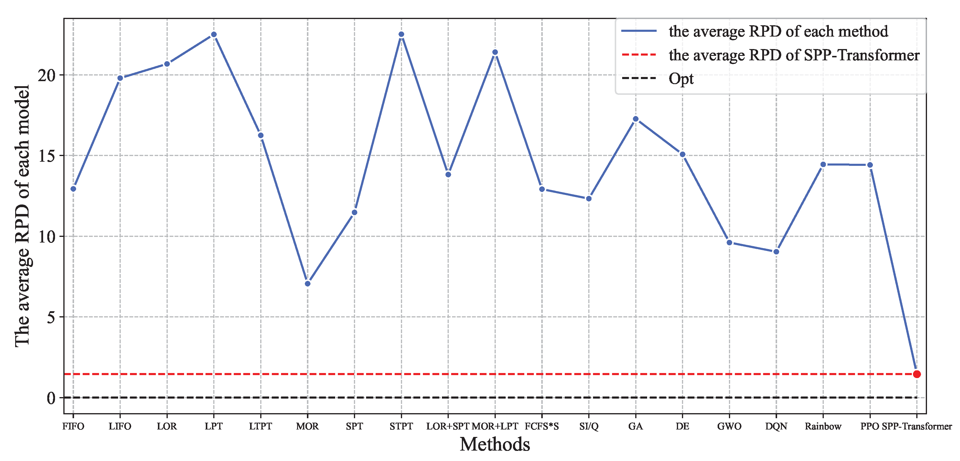
4.2. Performance Analysis
4.3. Data Ablation
5. Conclusions
Author Contributions
Funding
Institutional Review Board Statement
Informed Consent Statement
Data Availability Statement
Conflicts of Interest
Appendix A

| Instance | Size | Opt | Methods | ||||||||
|---|---|---|---|---|---|---|---|---|---|---|---|
| FIFO | LIFO | LOR | LPT | LTPT | MOR | SPT | STPT | SPP-Transformer | |||
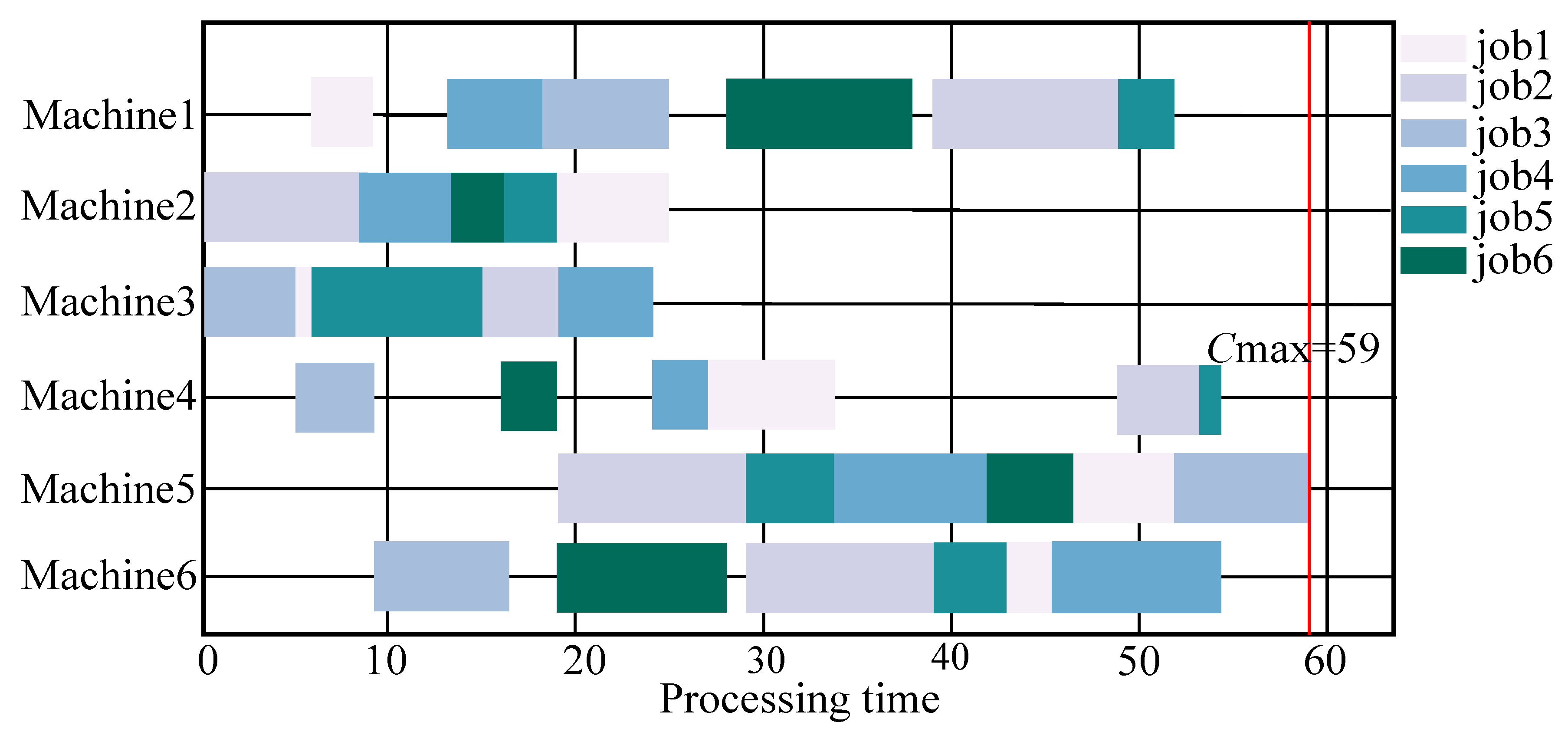
| FT06 | 6 × 6 | 59 | 65 | 70 | 68 | 77 | 68 | 59 | 88 | 83 | 59 |
| FT10 | 10 × 10 | 1002 | 1230 | 1201 | 1352 | 1295 | 1190 | 1163 | 1074 | 1262 | 1180 |
| FT20 | 5 × 20 | 1205 | 1658 | 1304 | 1487 | 1631 | 1495 | 1601 | 1267 | 1309 | 1231 |
| LA01 | 5 × 10 | 666 | 848 | 772 | 941 | 822 | 835 | 763 | 751 | 933 | 699 |
| LA02 | 5 × 10 | 684 | 821 | 799 | 982 | 990 | 881 | 812 | 821 | 761 | 716 |
| LA03 | 5 × 10 | 615 | 734 | 765 | 758 | 825 | 696 | 726 | 672 | 811 | 651 |
| LA04 | 5 × 10 | 615 | 737 | 827 | 745 | 818 | 887 | 706 | 711 | 874 | 670 |
| LA05 | 5 × 10 | 593 | 593 | 681 | 704 | 693 | 658 | 593 | 610 | 677 | 593 |
| LA06 | 5 × 15 | 926 | 1014 | 1246 | 1095 | 1125 | 1098 | 926 | 1200 | 1012 | 926 |
| LA07 | 5 × 15 | 920 | 1105 | 1156 | 1137 | 1069 | 1025 | 1001 | 1034 | 1105 | 956 |
| LA08 | 5 × 15 | 866 | 982 | 1101 | 995 | 1035 | 952 | 925 | 942 | 995 | 863 |
| LA09 | 5 × 15 | 952 | 1011 | 1089 | 1149 | 1183 | 1304 | 951 | 1045 | 1220 | 951 |
| LA10 | 5 × 15 | 958 | 1035 | 1132 | 1032 | 1132 | 1033 | 958 | 1049 | 1312 | 958 |
| LA11 | 5 × 20 | 1222 | 1229 | 1488 | 1586 | 1467 | 1416 | 1222 | 1473 | 1446 | 1222 |
| LA12 | 5 × 20 | 1039 | 1039 | 1329 | 1295 | 1240 | 1126 | 1039 | 1203 | 1358 | 1039 |
| LA13 | 5 × 20 | 1151 | 1160 | 1519 | 1320 | 1230 | 1252 | 1150 | 1275 | 1267 | 1150 |
| LA14 | 5 × 20 | 1292 | 1321 | 1505 | 1567 | 1434 | 1419 | 1292 | 1427 | 1646 | 1292 |
| LA15 | 5 × 20 | 1336 | 1471 | 1519 | 1598 | 1612 | 1394 | 1436 | 1339 | 1632 | 1321 |
| LA16 | 10 × 10 | 1108 | 1297 | 1306 | 1119 | 1229 | 1165 | 1108 | 1156 | 1268 | 1074 |
| LA17 | 10 × 10 | 844 | 908 | 987 | 948 | 1082 | 993 | 844 | 924 | 1120 | 812 |
| LA18 | 10 × 10 | 942 | 1057 | 1178 | 1154 | 1114 | 1198 | 942 | 981 | 1111 | 942 |
| LA19 | 10 × 10 | 952 | 1062 | 992 | 1004 | 1062 | 1004 | 1088 | 940 | 981 | 935 |
| LA20 | 10 × 10 | 1026 | 1243 | 1092 | 1207 | 1272 | 1086 | 1130 | 1000 | 1201 | 979 |
| Average | 912 | 1027 | 1089 | 1098 | 1106 | 1051 | 975 | 999 | 1104 | 923 | |
| Instance | Size | Methods | ||||||||
|---|---|---|---|---|---|---|---|---|---|---|
| FIFO | LIFO | LOR | LPT | LTPT | MOR | SPT | STPT | SPP-Transformer | ||
| FT06 | 6 × 6 | 10.17 | 18.64 | 15.25 | 30.51 | 15.25 | 0 | 49.15 | 40.68 | 0 |
| FT10 | 10 × 10 | 22.75 | 19.86 | 34.93 | 29.24 | 18.76 | 16.07 | 7.19 | 25.95 | 17.76 |
| FT20 | 5 × 20 | 37.59 | 8.22 | 23.4 | 35.35 | 24.07 | 32.86 | 5.15 | 8.63 | 2.16 |
| LA01 | 5 × 10 | 27.33 | 15.92 | 41.29 | 23.42 | 25.38 | 14.56 | 12.76 | 40.09 | 4.95 |
| LA02 | 5 × 10 | 20.03 | 16.81 | 43.57 | 44.74 | 28.8 | 18.71 | 20.03 | 11.26 | 4.68 |
| LA03 | 5 × 10 | 19.35 | 24.39 | 23.25 | 34.15 | 13.17 | 18.05 | 9.27 | 31.87 | 5.85 |
| LA04 | 5 × 10 | 19.84 | 34.47 | 21.14 | 33.01 | 44.23 | 14.8 | 15.61 | 42.11 | 8.94 |
| LA05 | 5 × 10 | 0 | 14.84 | 18.72 | 16.86 | 10.96 | 0 | 2.87 | 14.17 | 0 |
| LA06 | 5 × 15 | 9.5 | 34.56 | 18.25 | 21.49 | 18.57 | 0 | 29.59 | 9.29 | 0 |
| LA07 | 5 × 15 | 20.11 | 25.65 | 23.59 | 16.2 | 11.41 | 8.8 | 12.39 | 20.11 | 3.91 |
| LA08 | 5 × 15 | 13.39 | 27.14 | 14.9 | 19.52 | 9.93 | 6.81 | 8.78 | 14.9 | −0.35 |
| LA09 | 5 × 15 | 6.2 | 14.39 | 20.69 | 24.26 | 36.97 | −0.11 | 9.77 | 28.15 | −0.11 |
| LA10 | 5 × 15 | 8.04 | 18.16 | 7.72 | 18.16 | 7.83 | 0 | 9.5 | 36.95 | 0 |
| LA11 | 5 × 20 | 0.57 | 21.77 | 29.79 | 20.05 | 15.88 | 0 | 20.54 | 18.33 | 0 |
| LA12 | 5 × 20 | 0 | 27.91 | 24.64 | 19.35 | 8.37 | 0 | 15.78 | 30.7 | 0 |
| LA13 | 5 × 20 | 0.78 | 31.97 | 14.68 | 6.86 | 8.77 | −0.09 | 10.77 | 10.08 | −0.09 |
| LA14 | 5 × 20 | 2.24 | 16.49 | 21.28 | 10.99 | 9.83 | 0 | 10.45 | 27.4 | 0 |
| LA15 | 5 × 20 | 10.1 | 13.7 | 19.61 | 20.66 | 4.34 | 7.49 | 0.22 | 22.16 | −1.12 |
| LA16 | 10 × 10 | 17.06 | 17.87 | 0.99 | 10.92 | 5.14 | 0 | 4.33 | 14.44 | −3.07 |
| LA17 | 10 × 10 | 7.58 | 16.94 | 12.32 | 28.2 | 17.65 | 0 | 9.48 | 32.7 | −3.79 |
| LA18 | 10 × 10 | 12.21 | 25.05 | 22.51 | 18.26 | 27.18 | 0 | 4.14 | 17.94 | 0 |
| LA19 | 10 × 10 | 11.55 | 4.2 | 5.46 | 11.55 | 5.46 | 14.29 | −1.26 | 3.05 | −1.79 |
| LA20 | 10 × 10 | 21.15 | 6.43 | 17.64 | 23.98 | 5.85 | 10.14 | −2.53 | 17.06 | −4.58 |
| Average | 12.94 | 19.8 | 20.68 | 22.51 | 16.25 | 7.06 | 11.48 | 22.52 | 1.45 | |
| Instance | Size | Opt | Methods | ||||
|---|---|---|---|---|---|---|---|
| LOR+SPT | MOR+LPT | FCFS∗S | SI/Q | SPP-Transformer | |||
| FT06 | 6 × 6 | 59 | 85 | 68 | 78 | 84 | 59 |
| FT10 | 10 × 10 | 1002 | 1100 | 1284 | 1176 | 1114 | 1180 |
| FT20 | 5 × 20 | 1205 | 1280 | 1616 | 1358 | 1279 | 1231 |
| LA01 | 5 × 10 | 666 | 761 | 818 | 869 | 775 | 699 |
| LA02 | 5 × 10 | 684 | 796 | 952 | 773 | 778 | 716 |
| LA03 | 5 × 10 | 615 | 745 | 807 | 770 | 711 | 651 |
| LA04 | 5 × 10 | 615 | 703 | 865 | 722 | 698 | 670 |
| LA05 | 5 × 10 | 593 | 620 | 668 | 623 | 623 | 593 |
| LA06 | 5 × 15 | 926 | 1182 | 1122 | 1022 | 1171 | 926 |
| LA07 | 5 × 15 | 920 | 1021 | 1087 | 1082 | 1023 | 956 |
| LA08 | 5 × 15 | 866 | 959 | 1086 | 902 | 958 | 863 |
| LA09 | 5 × 15 | 952 | 1122 | 1178 | 1015 | 1060 | 951 |
| LA10 | 5 × 15 | 958 | 1090 | 1116 | 1041 | 1077 | 958 |
| LA11 | 5 × 20 | 1222 | 1494 | 1471 | 1318 | 1435 | 1222 |
| LA12 | 5 × 20 | 1039 | 1214 | 1245 | 1168 | 1227 | 1039 |
| LA13 | 5 × 20 | 1151 | 1338 | 1278 | 1234 | 1289 | 1150 |
| LA14 | 5 × 20 | 1292 | 1518 | 1405 | 1426 | 1463 | 1292 |
| LA15 | 5 × 20 | 1336 | 1356 | 1596 | 1429 | 1366 | 1321 |
| LA16 | 10 × 10 | 1108 | 1255 | 1219 | 1144 | 1181 | 1074 |
| LA17 | 10 × 10 | 844 | 956 | 1074 | 1001 | 944 | 812 |
| LA18 | 10 × 10 | 942 | 998 | 1099 | 1029 | 998 | 942 |
| LA19 | 10 × 10 | 952 | 950 | 1068 | 963 | 957 | 935 |
| LA20 | 10 × 10 | 1026 | 1022 | 1210 | 1223 | 1023 | 979 |
| Average | 912 | 1025 | 1101 | 1016 | 1010 | 923 | |
| Instance | Size | Methods | ||||
|---|---|---|---|---|---|---|
| LOR+SPT | MOR+LPT | FCFS∗S | SI/Q | SPP-Transformer | ||
| FT06 | 6 × 6 | 44.07 | 15.25 | 32.2 | 42.37 | 0 |
| FT10 | 10 × 10 | 9.78 | 28.14 | 17.37 | 11.18 | 17.76 |
| FT20 | 5 × 20 | 6.22 | 34.11 | 12.7 | 6.14 | 2.16 |
| LA11 | 5 × 10 | 14.26 | 22.82 | 30.48 | 16.37 | 4.95 |
| LA12 | 5 × 10 | 16.37 | 39.18 | 13.01 | 13.74 | 4.68 |
| LA13 | 5 × 10 | 21.14 | 31.22 | 25.2 | 15.61 | 5.85 |
| LA14 | 5 × 10 | 14.31 | 40.65 | 17.4 | 13.5 | 8.94 |
| LA15 | 5 × 10 | 4.55 | 12.65 | 5.06 | 5.06 | 0 |
| LA16 | 5 × 15 | 27.65 | 21.17 | 10.37 | 26.46 | 0 |
| LA17 | 5 × 15 | 10.98 | 18.15 | 17.61 | 11.2 | 3.91 |
| LA18 | 5 × 15 | 10.74 | 25.4 | 4.16 | 10.62 | −0.35 |
| LA19 | 5 × 15 | 17.86 | 23.74 | 6.62 | 11.34 | −0.11 |
| LA10 | 5 × 15 | 13.78 | 16.49 | 8.66 | 12.42 | 0 |
| LA11 | 5 × 20 | 22.26 | 20.38 | 7.86 | 17.43 | 0 |
| LA12 | 5 × 20 | 16.84 | 19.83 | 12.42 | 18.09 | 0 |
| LA13 | 5 × 20 | 16.25 | 11.03 | 7.21 | 11.99 | −0.09 |
| LA14 | 5 × 20 | 17.49 | 8.75 | 10.37 | 13.24 | 0 |
| LA15 | 5 × 20 | 1.5 | 19.46 | 6.96 | 2.25 | −1.12 |
| LA16 | 10 × 10 | 13.27 | 10.02 | 3.25 | 6.59 | −3.07 |
| LA17 | 10 × 10 | 13.27 | 27.25 | 18.6 | 11.85 | −3.79 |
| LA18 | 10 × 10 | 5.94 | 16.67 | 9.24 | 5.94 | 0 |
| LA19 | 10 × 10 | −0.21 | 12.18 | 1.16 | 0.53 | −1.79 |
| LA20 | 10 × 10 | −0.39 | 17.93 | 19.2 | −0.29 | −4.58 |
| Average | 13.82 | 21.41 | 12.92 | 12.33 | 1.45 | |
| Instance | Size | Opt | Methods | |||
|---|---|---|---|---|---|---|
| GA | DE | GWO | SPP-Transformer | |||
| FT06 | 6 × 6 | 59 | 58 | 60 | 59 | 59 |
| FT10 | 10 × 10 | 1002 | 1331 | 1312 | 1219 | 1180 |
| FT20 | 5 × 20 | 1205 | 1634 | 1635 | 1564 | 1231 |
| LA01 | 5 × 10 | 666 | 782 | 769 | 727 | 699 |
| LA02 | 5 × 10 | 684 | 821 | 805 | 768 | 716 |
| LA03 | 5 × 10 | 615 | 737 | 731 | 696 | 651 |
| LA04 | 5 × 10 | 615 | 736 | 728 | 681 | 670 |
| LA05 | 5 × 10 | 593 | 633 | 616 | 599 | 593 |
| LA06 | 5 × 15 | 926 | 1040 | 1025 | 982 | 926 |
| LA07 | 5 × 15 | 920 | 1085 | 1068 | 1014 | 956 |
| LA08 | 5 × 15 | 866 | 1045 | 1024 | 974 | 863 |
| LA09 | 5 × 15 | 952 | 1094 | 1063 | 1021 | 951 |
| LA10 | 5 × 15 | 958 | 1048 | 1020 | 985 | 958 |
| LA11 | 5 × 20 | 1222 | 1400 | 1371 | 1330 | 1222 |
| LA12 | 5 × 20 | 1039 | 1195 | 1182 | 1133 | 1039 |
| LA13 | 5 × 20 | 1151 | 1335 | 1312 | 1261 | 1150 |
| LA14 | 5 × 20 | 1292 | 1377 | 1352 | 1321 | 1292 |
| LA15 | 5 × 20 | 1336 | 1527 | 1498 | 1449 | 1321 |
| LA16 | 10 × 10 | 1108 | 1238 | 1206 | 1138 | 1074 |
| LA17 | 10 × 10 | 844 | 1072 | 1032 | 947 | 812 |
| LA18 | 10 × 10 | 942 | 1149 | 1109 | 1040 | 942 |
| LA19 | 10 × 10 | 952 | 1182 | 1142 | 1066 | 935 |
| LA20 | 10 × 10 | 1026 | 1235 | 1185 | 1118 | 979 |
| Average | 912 | 1076 | 1054 | 1004 | 923 | |
| Instance | Size | Methods | |||
|---|---|---|---|---|---|
| GA | DE | GWO | SPP-Transformer | ||
| FT06 | 6 × 6 | −1.69 | 1.69 | 0 | 0 |
| FT10 | 10 × 10 | 32.83 | 30.94 | 21.66 | 17.76 |
| FT20 | 5 × 20 | 35.6 | 35.68 | 29.79 | 2.16 |
| LA01 | 5 × 10 | 17.42 | 15.47 | 9.16 | 4.95 |
| LA02 | 5 × 10 | 20.03 | 17.69 | 12.28 | 4.68 |
| LA03 | 5 × 10 | 19.84 | 18.86 | 13.17 | 5.85 |
| LA04 | 5 × 10 | 19.67 | 18.37 | 10.73 | 8.94 |
| LA05 | 5 × 10 | 6.75 | 3.88 | 1.01 | 0 |
| LA06 | 5 × 15 | 12.31 | 10.69 | 6.05 | 0 |
| LA07 | 5 × 15 | 17.93 | 16.09 | 10.22 | 3.91 |
| LA08 | 5 × 15 | 20.67 | 18.24 | 12.47 | −0.35 |
| LA09 | 5 × 15 | 14.92 | 11.66 | 7.25 | −0.11 |
| LA10 | 5 × 15 | 9.39 | 6.47 | 2.82 | 0 |
| LA11 | 5 × 20 | 14.57 | 12.19 | 8.84 | 0 |
| LA12 | 5 × 20 | 15.01 | 13.76 | 9.05 | 0 |
| LA13 | 5 × 20 | 15.99 | 13.99 | 9.56 | −0.09 |
| LA14 | 5 × 20 | 6.58 | 4.64 | 2.24 | 0 |
| LA15 | 5 × 20 | 14.3 | 12.13 | 8.46 | −1.12 |
| LA16 | 10 × 10 | 11.73 | 8.84 | 2.71 | −3.07 |
| LA17 | 10 × 10 | 27.01 | 22.27 | 12.2 | −3.79 |
| LA18 | 10 × 10 | 21.97 | 17.73 | 10.4 | 0 |
| LA19 | 10 × 10 | 24.16 | 19.96 | 11.97 | −1.79 |
| LA20 | 10 × 10 | 20.37 | 15.5 | 8.97 | −4.58 |
| Average | 17.28 | 15.08 | 9.61 | 1.45 | |
| Instance | Size | Opt | Methods | |||
|---|---|---|---|---|---|---|
| DQN | Rainbow | PPO | SPP-Transformer | |||
| FT06 | 6 × 6 | 59 | 65 | 63 | 67 | 59 |
| FT10 | 10 × 10 | 1002 | 1289 | 1235 | 1341 | 1180 |
| FT20 | 5 × 20 | 1205 | 1463 | 1378 | 1479 | 1231 |
| LA01 | 5 × 10 | 666 | 785 | 935 | 759 | 699 |
| LA02 | 5 × 10 | 684 | 809 | 804 | 851 | 716 |
| LA03 | 5 × 10 | 615 | 750 | 742 | 713 | 651 |
| LA04 | 5 × 10 | 615 | 684 | 812 | 779 | 670 |
| LA05 | 5 × 10 | 593 | 592 | 660 | 634 | 593 |
| LA06 | 5 × 15 | 926 | 984 | 1066 | 963 | 926 |
| LA07 | 5 × 15 | 920 | 1035 | 991 | 1034 | 956 |
| LA08 | 5 × 15 | 866 | 1014 | 964 | 1125 | 863 |
| LA09 | 5 × 15 | 952 | 1010 | 1121 | 987 | 951 |
| LA10 | 5 × 15 | 958 | 978 | 1045 | 1021 | 958 |
| LA11 | 5 × 20 | 1222 | 1283 | 1480 | 1314 | 1222 |
| LA12 | 5 × 20 | 1039 | 1123 | 1204 | 1121 | 1039 |
| LA13 | 5 × 20 | 1151 | 1198 | 1300 | 1243 | 1150 |
| LA14 | 5 × 20 | 1292 | 1283 | 1290 | 1324 | 1292 |
| LA15 | 5 × 20 | 1336 | 1390 | 1393 | 1516 | 1321 |
| LA16 | 10 × 10 | 1108 | 1102 | 1183 | 1179 | 1074 |
| LA17 | 10 × 10 | 844 | 894 | 900 | 987 | 812 |
| LA18 | 10 × 10 | 942 | 993 | 1147 | 1123 | 942 |
| LA19 | 10 × 10 | 952 | 963 | 958 | 1146 | 935 |
| LA20 | 10 × 10 | 1026 | 1047 | 1183 | 1178 | 979 |
| Average | 912 | 988 | 1037 | 1038 | 923 | |
| Instance | Size | Methods | |||
|---|---|---|---|---|---|
| DQN | Rainbow | PPO | SPP-Transformer | ||
| FT06 | 6 × 6 | 10.17 | 6.78 | 13.56 | 0 |
| FT10 | 10 × 10 | 28.64 | 23.25 | 33.83 | 17.76 |
| FT20 | 5 × 20 | 21.41 | 14.36 | 22.74 | 2.16 |
| LA01 | 5 × 10 | 17.87 | 40.39 | 13.96 | 4.95 |
| LA02 | 5 × 10 | 18.27 | 17.54 | 24.42 | 4.68 |
| LA03 | 5 × 10 | 21.95 | 20.65 | 15.93 | 5.85 |
| LA04 | 5 × 10 | 11.22 | 32.03 | 26.67 | 8.94 |
| LA05 | 5 × 10 | −0.17 | 11.3 | 6.91 | 0 |
| LA06 | 5 × 15 | 6.26 | 15.12 | 4 | 0 |
| LA07 | 5 × 15 | 12.5 | 7.72 | 12.39 | 3.91 |
| LA08 | 5 × 15 | 17.09 | 11.32 | 29.91 | −0.35 |
| LA09 | 5 × 15 | 6.09 | 17.75 | 3.68 | −0.11 |
| LA10 | 5 × 15 | 2.09 | 9.08 | 6.58 | 0 |
| LA11 | 5 × 20 | 4.99 | 21.11 | 7.53 | 0 |
| LA12 | 5 × 20 | 8.08 | 15.88 | 7.89 | 0 |
| LA13 | 5 × 20 | 4.08 | 12.95 | 7.99 | −0.09 |
| LA14 | 5 × 20 | −0.7 | −0.15 | 2.48 | 0 |
| LA15 | 5 × 20 | 4.04 | 4.27 | 13.47 | −1.12 |
| LA16 | 10 × 10 | −0.54 | 6.77 | 6.41 | −3.07 |
| LA17 | 10 × 10 | 5.92 | 6.64 | 16.94 | −3.79 |
| LA18 | 10 × 10 | 5.41 | 21.76 | 19.21 | 0 |
| LA19 | 10 × 10 | 1.16 | 0.63 | 20.38 | −1.79 |
| LA20 | 10 × 10 | 2.05 | 15.3 | 14.81 | −4.58 |
| Average | 9.04 | 14.45 | 14.42 | 1.45 | |
Appendix B
| Instance | Size | Opt | Methods | ||
|---|---|---|---|---|---|
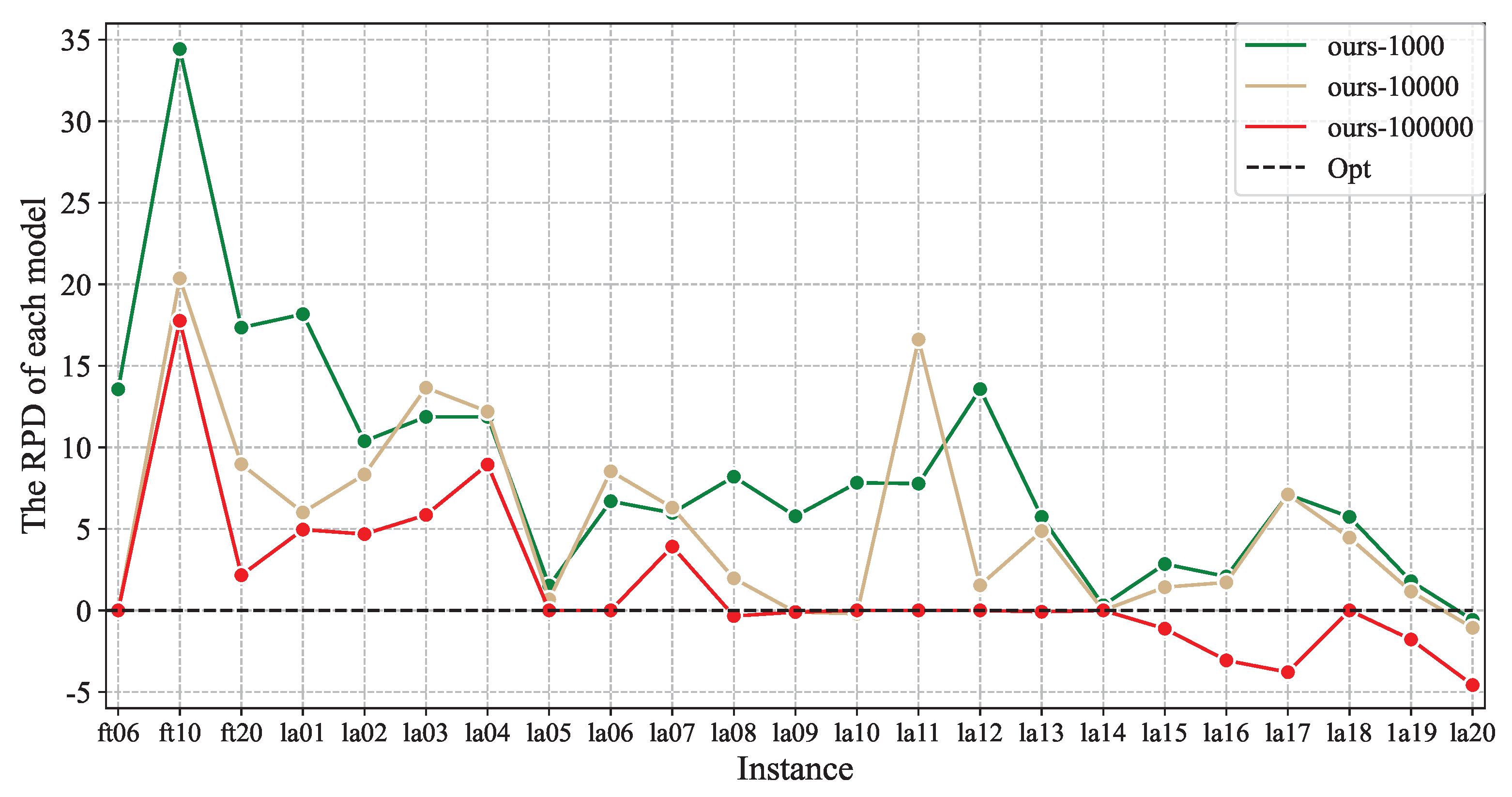
| Ours-1000 | Ours-10000 | Ours-100000 | |||
| FT06 | 6 × 6 | 59 | 67 | 59 | 59 |
| FT10 | 10 × 10 | 1002 | 1347 | 1206 | 1180 |
| FT20 | 5 × 20 | 1205 | 1414 | 1313 | 1231 |
| LA01 | 5 × 10 | 666 | 787 | 706 | 699 |
| LA02 | 5 × 10 | 684 | 755 | 741 | 716 |
| LA03 | 5 × 10 | 615 | 688 | 699 | 651 |
| LA04 | 5 × 10 | 615 | 688 | 690 | 670 |
| LA05 | 5 × 10 | 593 | 602 | 597 | 593 |
| LA06 | 5 × 15 | 926 | 988 | 1005 | 926 |
| LA07 | 5 × 15 | 920 | 975 | 978 | 956 |
| LA08 | 5 × 15 | 866 | 937 | 883 | 863 |
| LA09 | 5 × 15 | 952 | 1007 | 951 | 951 |
| LA10 | 5 × 15 | 958 | 1033 | 956 | 958 |
| LA11 | 5 × 20 | 1222 | 1317 | 1425 | 1222 |
| LA12 | 5 × 20 | 1039 | 1180 | 1055 | 1039 |
| LA13 | 5 × 20 | 1151 | 1217 | 1207 | 1150 |
| LA14 | 5 × 20 | 1292 | 1296 | 1292 | 1292 |
| LA15 | 5 × 20 | 1336 | 1374 | 1355 | 1321 |
| LA16 | 10 × 10 | 1108 | 1131 | 1127 | 1074 |
| LA17 | 10 × 10 | 844 | 904 | 904 | 812 |
| LA18 | 10 × 10 | 942 | 996 | 984 | 942 |
| LA19 | 10 × 10 | 952 | 969 | 963 | 935 |
| LA20 | 10 × 10 | 1026 | 1020 | 1015 | 979 |
| Average | 912 | 988 | 1037 | 923 | |
| Instance | Size | Methods | ||
|---|---|---|---|---|
| Ours-1000 | Ours-10000 | Ours-100000 | ||
| FT06 | 6 × 6 | 13.56 | 0 | 0 |
| FT10 | 10 × 10 | 34.43 | 20.36 | 17.76 |
| FT20 | 5 × 20 | 17.34 | 8.96 | 2.16 |
| LA01 | 5 × 10 | 18.17 | 6.01 | 4.95 |
| LA02 | 5 × 10 | 10.38 | 8.33 | 4.68 |
| LA03 | 5 × 10 | 11.87 | 13.66 | 5.85 |
| LA04 | 5 × 10 | 11.87 | 12.2 | 8.94 |
| LA05 | 5 × 10 | 1.52 | 0.67 | 0 |
| LA06 | 5 × 15 | 6.7 | 8.53 | 0 |
| LA07 | 5 × 15 | 5.98 | 6.3 | 3.91 |
| LA08 | 5 × 15 | 8.2 | 1.96 | −0.35 |
| LA09 | 5 × 15 | 5.78 | −0.11 | −0.11 |
| LA10 | 5 × 15 | 7.83 | −0.21 | 0 |
| LA11 | 5 × 20 | 7.77 | 16.61 | 0 |
| LA12 | 5 × 20 | 13.57 | 1.54 | 0 |
| LA13 | 5 × 20 | 5.73 | 4.87 | −0.09 |
| LA14 | 5 × 20 | 0.31 | 0 | 0 |
| LA15 | 5 × 20 | 2.84 | 1.42 | −1.12 |
| LA16 | 10 × 10 | 2.08 | 1.71 | −3.07 |
| LA17 | 10 × 10 | 7.11 | 7.11 | −3.79 |
| LA18 | 10 × 10 | 5.73 | 4.46 | 0 |
| LA19 | 10 × 10 | 1.79 | 1.16 | −1.79 |
| LA20 | 10 × 10 | −0.58 | −1.07 | −4.58 |
| Average | 8.69 | 5.41 | 1.45 | |
References
- Ma, J.; Chen, H.; Zhang, Y.; Guo, H.; Ren, Y.; Mo, R.; Liu, L. A digital twin-driven production management system for production workshop. Int. J. Adv. Manuf. Technol. 2020, 110, 1385–1397. [Google Scholar] [CrossRef]
- Guo, H.; Zhu, Y.; Zhang, Y.; Ren, Y.; Chen, M.; Zhang, R. A digital twin-based layout optimization method for discrete manufacturing workshop. Int. J. Adv. Manuf. Technol. 2021, 112, 1307–1318. [Google Scholar] [CrossRef]
- Garey, M.R.; Johnson, D.S.; Sethi, R. The complexity of flowshop and jobshop scheduling. Math. Oper. Res. 1976, 1, 117–129. [Google Scholar] [CrossRef]
- Renke, L.; Piplani, R.; Toro, C. A Review of Dynamic Scheduling: Context, Techniques and Prospects. J. Intell. Syst. Ref. Libr. Implement. Ind. 2021, 4, 229–258. [Google Scholar] [CrossRef]
- Tay, J.C.; Ho, N.B. Evolving dispatching rules using genetic programming for solving multi-objective flexible job-shop problems. Comput. Ind. Eng. 2008, 54, 453–473. [Google Scholar] [CrossRef] [Green Version]
- Papakostas, N.; Chryssolouris, G. A scheduling policy for improving tardiness performance. Asian Int. J. Sci. Technol. 2009, 2, 79–89. [Google Scholar]
- Cheng, R.; Gen, M.; Tsujimura, Y. A tutorial survey of job-shop scheduling problems using genetic algorithms—I. Representation. Comput. Ind. Eng. 1996, 30, 983–997. [Google Scholar] [CrossRef]
- Wong, K.P.; Dong, Z.Y. Differential evolution, an alternative approach to evolutionary algorithm. In Proceedings of the 13th International Conference on Intelligent Systems Application to Power Systems, Arlington, VA, USA, 6–10 November 2005; pp. 73–83. [Google Scholar]
- Mirjalili, S.; Mirjalili, S.M.; Lewis, A. Grey wolf optimizer. Adv. Eng. Softw. 2014, 69, 46–61. [Google Scholar] [CrossRef] [Green Version]
- Zhou, R.; Nee, A.; Lee, H. Performance of an ant colony optimisation algorithm in dynamic job shop scheduling problems. Int. J. Prod. Res. 2009, 47, 2903–2920. [Google Scholar] [CrossRef]
- Wang, Z.; Zhang, J.; Yang, S. An improved particle swarm optimization algorithm for dynamic job shop scheduling problems with random job arrivals. Swarm Evol. Comput. 2019, 51, 100594. [Google Scholar] [CrossRef]
- Mazyavkina, N.; Sviridov, S.; Ivanov, S.; Burnaev, E. Reinforcement learning for combinatorial optimization: A survey. Comput. Oper. Res. 2021, 134, 105400. [Google Scholar] [CrossRef]
- Wang, F.Y.; Zhang, J.J.; Zheng, X.; Wang, X.; Yuan, Y.; Dai, X.; Zhang, J.; Yang, L. Where does AlphaGo go: From church-turing thesis to AlphaGo thesis and beyond. IEEE/CAA J. Autom. Sin. 2016, 3, 113–120. [Google Scholar] [CrossRef]
- Jumper, J.; Evans, R.; Pritzel, A.; Green, T.; Figurnov, M.; Ronneberger, O.; Tunyasuvunakool, K.; Bates, R.; Žídek, A.; Potapenko, A.; et al. Highly accurate protein structure prediction with AlphaFold. Nature 2021, 596, 583–589. [Google Scholar] [CrossRef] [PubMed]
- Rinciog, A.; Meyer, A. Towards Standardizing Reinforcement Learning Approaches for Stochastic Production Scheduling. arXiv 2021, arXiv:2104.08196. [Google Scholar] [CrossRef]
- Zhou, T.; Tang, D.; Zhu, H.; Wang, L. Reinforcement learning with composite rewards for production scheduling in a smart factory. IEEE Access 2020, 9, 752–766. [Google Scholar] [CrossRef]
- Turgut, Y.; Bozdag, C.E. Deep Q-network model for dynamic job shop scheduling pproblem based on discrete event simulation. In Proceedings of the 2020 Winter Simulation Conference (WSC), Orlando, FL, USA, 14–18 December 2020; pp. 1551–1559. [Google Scholar]
- Wang, L.; Hu, X.; Wang, Y.; Xu, S.; Ma, S.; Yang, K.; Liu, Z.; Wang, W. Dynamic job-shop scheduling in smart manufacturing using deep reinforcement learning. Comput. Netw. 2021, 190, 107969. [Google Scholar] [CrossRef]
- Liu, C.L.; Chang, C.C.; Tseng, C.J. Actor-critic deep reinforcement learning for solving job shop scheduling problems. IEEE Access 2020, 8, 71752–71762. [Google Scholar] [CrossRef]
- Ghosh, D.; Rahme, J.; Kumar, A.; Zhang, A.; Adams, R.P.; Levine, S. Why Generalization in RL is Difficult: Epistemic POMDPs and Implicit Partial Observability. In Proceedings of the Advances in Neural Information Processing Systems, Virtual, 6–14 December 2021; pp. 25502–25515. [Google Scholar]
- Weckman, G.R.; Ganduri, C.V.; Koonce, D.A. A neural network job-shop scheduler. J. Intell. Manuf. 2008, 19, 191–201. [Google Scholar] [CrossRef]
- Sim, M.H.; Low, M.Y.H.; Chong, C.S.; Shakeri, M. Job Shop Scheduling Problem Neural Network Solver with Dispatching Rules. In Proceedings of the 2020 IEEE International Conference on Industrial Engineering and Engineering Management (IEEM), Singapore, 14–17 December 2020; pp. 514–518. [Google Scholar]
- Zang, Z.; Wang, W.; Song, Y.; Lu, L.; Li, W.; Wang, Y.; Zhao, Y. Hybrid deep neural network scheduler for job-shop problem based on convolution two-dimensional transformation. Comput. Intell. Neurosci. 2019, 2019, 7172842. [Google Scholar] [CrossRef] [Green Version]
- Tian, W.; Zhang, H. A dynamic job-shop scheduling model based on deep learning. Adv. Prod. Eng. Manag. 2021, 16, 23–36. [Google Scholar] [CrossRef]
- Shao, X.; Kim, C.S. Self-Supervised Long-Short Term Memory Network for Solving Complex Job Shop Scheduling Problem. KSII Trans. Internet Inf. Syst. (TIIS) 2021, 15, 2993–3010. [Google Scholar] [CrossRef]
- Morariu, C.; Borangiu, T. Time series forecasting for dynamic scheduling of manufacturing processes. In Proceedings of the 2018 IEEE International Conference on Automation, Quality and Testing, Robotics (AQTR), Cluj-Napoca, Romania, 24–26 May 2018; pp. 1–6. [Google Scholar]
- Zhou, H.; Zhang, S.; Peng, J.; Zhang, S.; Li, J.; Xiong, H.; Zhang, W. Informer: Beyond Efficient Transformer for Long Sequence Time-Series Forecasting. In Proceedings of the AAAI Conference on Artificial Intelligence, Vancouver, BC, Canada, 2–9 February 2021; pp. 11106–11115. [Google Scholar]
- Magalhães, R.; Martins, M.; Vieira, S.; Santos, F.; Sousa, J. Encoder-Decoder Neural Network Architecture for solving Job Shop Scheduling Problems using Reinforcement Learning. In Proceedings of the 2021 IEEE Symposium Series on Computational Intelligence (SSCI), Orlando, FL, USA, 5–7 December 2021; pp. 1–8. [Google Scholar]
- Yang, S. Using Attention Mechanism to Solve Job Shop Scheduling Problem. In Proceedings of the 2022 2nd International Conference on Consumer Electronics and Computer Engineering (ICCECE), Guangzhou, China, 14–16 January 2022; pp. 59–62. [Google Scholar]
- Chen, R.; Li, W.; Yang, H. A Deep Reinforcement Learning Framework Based on an Attention Mechanism and Disjunctive Graph Embedding for the Job Shop Scheduling Problem. IEEE Trans. Ind. Inform. 2022, 1. [Google Scholar] [CrossRef]
- Shakhlevich, N.; Sotskov, Y.N.; Werner, F. Adaptive scheduling algorithm based on mixed graph model. IEE Proc.-Control Theory Appl. 1996, 43, 9–16. [Google Scholar] [CrossRef]
- Gholami, O.; Sotskov, Y.N. Solving parallel machines job-shop scheduling problems by an adaptive algorithm. Int. J. Prod. Res. 2014, 52, 3888–3904. [Google Scholar] [CrossRef]
- He, K.; Zhang, X.; Ren, S.; Sun, J. Spatial pyramid pooling in deep convolutional networks for visual recognition. IEEE Trans. Pattern Anal. Mach. Intell. 2015, 37, 1904–1916. [Google Scholar] [CrossRef] [Green Version]
- Wang, Z.; Zhang, J.; Si, J. Dynamic job shop scheduling problem with new job arrivals: A survey. In Proceedings of the Chinese Intelligent Automation Conference, Zhenjiang, China, 20–22 September 2019; pp. 664–671. [Google Scholar]
- Błażewicz, J.; Pesch, E.; Sterna, M. The disjunctive graph machine representation of the job shop scheduling problem. Eur. J. Oper. Res. 2000, 127, 317–331. [Google Scholar] [CrossRef]
- Zeng, Y.; Liao, Z.; Dai, Y.; Wang, R.; Li, X.; Yuan, B. Hybrid intelligence for dynamic job-shop scheduling with deep reinforcement learning and attention mechanism. arXiv 2022, arXiv:2201.00548. [Google Scholar] [CrossRef]
- Chen, B.; Matis, T.I. A flexible dispatching rule for minimizing tardiness in job shop scheduling. Int. J. Prod. Econ. 2013, 141, 360–365. [Google Scholar] [CrossRef]
- He, K.; Zhang, X.; Ren, S.; Sun, J. Deep residual learning for image recognition. In Proceedings of the IEEE Conference on Computer Vision and Pattern Recognition, Las Vegas, NV, USA, 27–30 June 2016; pp. 770–778. [Google Scholar]
- Ba, J.L.; Kiros, J.R.; Hinton, G.E. Layer normalization. arXiv 2016, arXiv:1607.06450. [Google Scholar] [CrossRef]
- Wang, Y.; Mohamed, A.; Le, D.; Liu, C.; Xiao, A.; Mahadeokar, J.; Huang, H.; Tjandra, A.; Zhang, X.; Zhang, F.; et al. Transformer-based acoustic modeling for hybrid speech recognition. In Proceedings of the ICASSP 2020—2020 IEEE International Conference on Acoustics, Speech and Signal Processing (ICASSP), Barcelona, Spain, 4–8 May 2020; pp. 6874–6878. [Google Scholar]
- Vaswani, A.; Shazeer, N.; Parmar, N.; Uszkoreit, J.; Jones, L.; Gomez, A.N.; Kaiser, L.u.; Polosukhin, I. Attention is All you Need. In Proceedings of the Advances in Neural Information Processing Systems, Long Beach, CA, USA, 4–9 December 2017; pp. 5998–6008. [Google Scholar]
- Beasley, J.E. OR-Library: Distributing test problems by electronic mail. J. Oper. Res. Soc. 1990, 41, 1069–1072. [Google Scholar] [CrossRef]
- Fisher, H. Probabilistic Learning Combinations of Local Job-Shop Scheduling Rules; Prentice-Hall: Hoboken, NJ, USA, 1963; pp. 225–251. [Google Scholar]
- Lawrence, S. Resouce Constrained Project Scheduling: An Experimental Investigation of Heuristic Scheduling Techniques (Supplement); Graduate School of Industrial Administration, Carnegie-Mellon University: Pittsburgh, PA, USA, 1984. [Google Scholar]
- Available online: https://github.com/Yunhui1998/TOFA (accessed on 27 April 2022).
- Hessel, M.; Modayil, J.; Van Hasselt, H.; Schaul, T.; Ostrovski, G.; Dabney, W.; Horgan, D.; Piot, B.; Azar, M.; Silver, D. Rainbow: Combining improvements in deep reinforcement learning. In Proceedings of the Thirty-Second AAAI Conference on Artificial Intelligence, New Orleans, LA, USA, 2–7 February 2018; pp. 3215–3222. [Google Scholar]
- Schulman, J.; Wolski, F.; Dhariwal, P.; Radford, A.; Klimov, O. Proximal policy optimization algorithms. arXiv 2017, arXiv:1707.06347. [Google Scholar] [CrossRef]
- Zhang, W.; Wen, J.; Zhu, Y.; Hu, Y. Multi-objective scheduling simulation of flexible job-shop based on multi-population genetic algorithm. Int. J. Simul. Model. 2017, 16, 313–321. [Google Scholar] [CrossRef]
- Dosovitskiy, A.; Beyer, L.; Kolesnikov, A.; Weissenborn, D.; Zhai, X.; Unterthiner, T.; Dehghani, M.; Minderer, M.; Heigold, G.; Gelly, S.; et al. An image is worth 16x16 words: Transformers for image recognition at scale. arXiv 2020, arXiv:2010.11929. [Google Scholar] [CrossRef]


| Parameters | Description |
|---|---|
| i | index of jobs, |
| j | index of operations of a job, |
| m | the number of machines |
| the maximum completion time of all jobs | |
| the start time of operation | |
| the end time of operation | |
| the end time of operation | |
| the processing time of operation | |
| T | the maximum total number of all planned operations at the current time |
| Hyperparameter | Value |
|---|---|
| Number of encoder layers | 6 |
| Number of decoder layers | 6 |
| Number of feed-forward network layers | 1 |
| Random rate f | 0.1 |
| True | |
| Number of heads | 8 |
| Number of training epochs | 10,000 |
| Number of test epochs | 100 |
| Optimizer | Adam |
| Mini-batch size | 128 |
| Dropout rate | 0.1 |
| Instance | Size | Opt | Methods | |||||||||
|---|---|---|---|---|---|---|---|---|---|---|---|---|
| Simple Priority Rules | Composite Dispatching Rules | Meta-Heuristic Methods | RL Methods | SPP-Transformer | ||||||||
| Makespan | RPD | Makespan | RPD | Makespan | RPD | Makespan | RPD | Makespan | RPD | |||
| FT06 | 6 × 6 | 59 | 72 | 22.46 | 79 | 33.47 | 59 | 0 | 65 | 10.17 | 59 | 0 |
| FT10 | 10 × 10 | 1002 | 1221 | 21.84 | 1169 | 16.62 | 1287 | 28.48 | 1288 | 28.57 | 1180 | 17.76 |
| FT20 | 5 × 20 | 1205 | 1469 | 21.91 | 1383 | 14.79 | 1611 | 33.69 | 1440 | 19.5 | 1231 | 2.16 |
| LA01 | 5 × 10 | 666 | 833 | 25.09 | 806 | 20.98 | 759 | 14.02 | 826 | 24.07 | 699 | 4.95 |
| LA02 | 5 × 10 | 684 | 858 | 25.49 | 825 | 20.58 | 798 | 16.67 | 821 | 20.08 | 716 | 4.68 |
| LA03 | 5 × 10 | 615 | 748 | 21.69 | 758 | 23.29 | 721 | 17.29 | 735 | 19.51 | 651 | 5.85 |
| LA04 | 5 × 10 | 615 | 788 | 28.15 | 747 | 21.47 | 715 | 16.26 | 758 | 23.31 | 670 | 8.94 |
| LA05 | 5 × 10 | 593 | 651 | 9.8 | 634 | 6.83 | 616 | 3.88 | 629 | 6.01 | 593 | 0 |
| LA06 | 5 × 15 | 926 | 1090 | 17.66 | 1124 | 21.41 | 1016 | 9.68 | 1004 | 8.46 | 926 | 0 |
| LA07 | 5 × 15 | 920 | 1079 | 17.28 | 1053 | 14.49 | 1056 | 14.75 | 1020 | 10.87 | 956 | 3.91 |
| LA08 | 5 × 15 | 866 | 991 | 14.42 | 976 | 12.73 | 1014 | 17.13 | 1034 | 19.44 | 863 | −0.35 |
| LA09 | 5 × 15 | 952 | 1119 | 17.54 | 1094 | 14.89 | 1059 | 11.28 | 1039 | 9.17 | 951 | −0.11 |
| LA10 | 5 × 15 | 958 | 1085 | 13.3 | 1081 | 12.84 | 1018 | 6.23 | 1015 | 5.92 | 958 | 0 |
| LA11 | 5 × 20 | 1222 | 1416 | 15.87 | 1430 | 16.98 | 1367 | 11.87 | 1359 | 11.21 | 1222 | 0 |
| LA12 | 5 × 20 | 1039 | 1204 | 15.84 | 1214 | 16.8 | 1170 | 12.61 | 1149 | 10.62 | 1039 | 0 |
| LA13 | 5 × 20 | 1151 | 1272 | 10.48 | 1285 | 11.62 | 1303 | 13.18 | 1247 | 8.34 | 1150 | −0.09 |
| LA14 | 5 × 20 | 1292 | 1451 | 12.34 | 1453 | 12.46 | 1350 | 4.49 | 1299 | 0.54 | 1292 | 0 |
| LA15 | 5 × 20 | 1336 | 1500 | 12.29 | 1437 | 7.54 | 1491 | 11.63 | 1433 | 7.26 | 1321 | −1.12 |
| LA16 | 10 × 10 | 1108 | 1206 | 8.84 | 1200 | 8.28 | 1194 | 7.76 | 1155 | 4.21 | 1074 | −3.07 |
| LA17 | 10 × 10 | 844 | 976 | 15.61 | 994 | 17.74 | 1017 | 20.49 | 927 | 9.83 | 812 | −3.79 |
| LA18 | 10 × 10 | 942 | 1092 | 15.91 | 1031 | 9.45 | 1099 | 16.7 | 1088 | 15.46 | 942 | 0 |
| LA19 | 10 × 10 | 952 | 1017 | 6.79 | 985 | 3.42 | 1130 | 18.7 | 1022 | 7.39 | 935 | −1.79 |
| LA20 | 10 × 10 | 1026 | 1154 | 12.47 | 1120 | 9.11 | 1179 | 14.95 | 1136 | 10.72 | 979 | −4.58 |
| Average | 912 | 1056 | 16.66 | 1038 | 15.12 | 1045 | 13.99 | 1021 | 12.64 | 923 | 1.45 | |
Publisher’s Note: MDPI stays neutral with regard to jurisdictional claims in published maps and institutional affiliations. |
© 2022 by the authors. Licensee MDPI, Basel, Switzerland. This article is an open access article distributed under the terms and conditions of the Creative Commons Attribution (CC BY) license (https://creativecommons.org/licenses/by/4.0/).
Share and Cite
Chen, S.; Huang, Z.; Guo, H. An End-to-End Deep Learning Method for Dynamic Job Shop Scheduling Problem. Machines 2022, 10, 573. https://doi.org/10.3390/machines10070573
Chen S, Huang Z, Guo H. An End-to-End Deep Learning Method for Dynamic Job Shop Scheduling Problem. Machines. 2022; 10(7):573. https://doi.org/10.3390/machines10070573
Chicago/Turabian StyleChen, Shifan, Zuyi Huang, and Hongfei Guo. 2022. "An End-to-End Deep Learning Method for Dynamic Job Shop Scheduling Problem" Machines 10, no. 7: 573. https://doi.org/10.3390/machines10070573