Article

3D Pipe Forming of a New Bending Machine with a 3PUU–3RPS Hybrid Mechanism

1
School of Mechanical, Electrical and Information Engineering, Shandong University at Weihai, Weihai 264209, China
2
GAMMA3-INRIA/ICD, University of Technology of Troyes, 10010 Troyes, France
3
Sino-French International Joint Research Laboratory of Computing Technology for Advanced Materials, Shanghai 200240, China
*
Author to whom correspondence should be addressed.
These authors contributed equally to this work.
Machines 2022, 10(6), 470; https://doi.org/10.3390/machines10060470
Submission received: 7 May 2022 / Revised: 3 June 2022 / Accepted: 9 June 2022 / Published: 12 June 2022
(This article belongs to the Topic Designs and Drive Control of Electromechanical Machines)

Abstract

:
To achieve the spatial variable curvature bending process of metal pipes, one 3PUU–3RPS hybrid mechanism designed for the free-bending forming of pipes is presented in this study. Its kinematics model was conducted based on theoretical analysis, and the obtained result was validated through ADAMS simulation. Through the theoretical analysis, the inverse position model of the proposed mechanical construction, which can show the relationship between the motion and the drive of the working platform, was presented. The velocity Jacobian matrix was also obtained and analyzed by establishing the inverse velocity model and inverse acceleration model. In addition, the static stiffness analysis of the proposed mechanical construction was also conducted in ABAQUS. Finally, by investigating its working space, the capability of 3PUU–3RPS mechanism was proved.

1. Introduction

The metal pipe not only has good forming property, but also has the characteristics of high strength, high stiffness, and high material utilization [1]. Therefore, the metal pipe has important applications in various industrial fields, such as electric power construction, railway construction, ships, furniture, and other areas of infrastructure. In aerospace, the metal pipe is also widely used in large precision machinery equipment and other high-end areas [2,3]. Therefore, many researchers are studying the precise forming of the metal pipe. H. Li et al. [4] established an AFE-based hybrid analytical-numerical framework for neutral layer shifting (NLS) calculation in tube bending. J. Wu et al. [5] proposed a new comprehensive strategy for the springback control of 3D tubes. J. Ma et al. [6] developed a generalized analytical model to accurately analyze springback in the bending of tubular materials. H. Yang et al. [7] developed a differential heating-based bending method to break the forming limit of difficult-to-form tubular materials. In the past few years, many efforts have been made to predict and compensate for springback [8,9,10,11,12].
However, among the manufacturing processes of metal pipes, the common bending forming methods include roll bending, draw bending, press bending, push bending and rotary-draw bending, etc. [13]. At present, with the developing requirement on the directions of lightweight miniaturization and integration of aerospace products, the space complexity and forming precision of pipeline are greatly improved, and higher requirements for the production of bending pipes are given. In order to meet these requirements, some new forming devices for metal pipes have to been developed [14,15].
To overcome the shortcomings of traditional bending methods, some ways to realize the spatial variable curvature-bending forming have been gradually developed [16]. As a new technology, 3D free-bending technology has the great potential to be suitable for the most tubes and profiles because of its geometrical flexibility and efficiency [17]. Plettke et al. [18] proposed a new method (free bending) which is suitable for arbitrary curve forming in space. The key point of this method is to gradually push the pipe through a bending die which can rotate freely within a certain angle of space. The shape of the bent pipe is controlled by adjusting the rotation of the mobile die. Free bending permits bending of almost all geometries. However, the minimum bending radius is approximately 2.5 times the pipe diameter, and it is also sensitive to the changes in material property.
P. Gantner et al. [19] developed a new bending technique in the hydroforming process chain, which is particularly suitable for the bending profile and tube cross-sections and has advantageous characteristics, such as fast bending speeds and an almost free definable bending geometry with transitionless bend-in-bends and spline bends without re-clamping.
S. Chatti et al. [20] carried out the numerical simulation studies on the torque superposed spatial bending (TSS) [21,22] and three-roll bending [23,24] processes. Based on the roll-bending process, dynamically adjusting the bending profile and superposing torque, controlling forming process parameters are given to achieve the purpose of bending different radii and angles.
H. Goto et al. [25,26] proposed a new type of multifunctional pipe-bending machine. By feeding the pipe into the fixed die and mobile die, adjusting the position of the mobile die can achieve bending. The bending radius is controlled by the relative distance and direction of the mobile die with the fixed die, and the bending angle is controlled by adjusting the feed length of the pipe. The movement of the mobile die is controlled by 6-DOF parallel kinematics (PKM).
Combining serial mechanisms with parallel mechanisms can allow these mechanisms to take full advantages of each other. Therefore, this paper proposes a new type of hybrid mechanism with 3PUU–3RPS structure which can better serve the needs of the spatial variable curvature bending of the metal pipe. The analysis of degrees of freedom, inverse position calculation, the analysis of kinematics and dynamics, stiffness analysis, workspace analysis, and other aspects of the new hybrid mechanism are studied. It turns out that the hybrid mechanism has less cumulative error, higher stiffness, and higher loading capacity than the series mechanism. Compared with the traditional parallel mechanism, the hybrid mechanism is easier to realize real-time control, and its workspace is also increased.

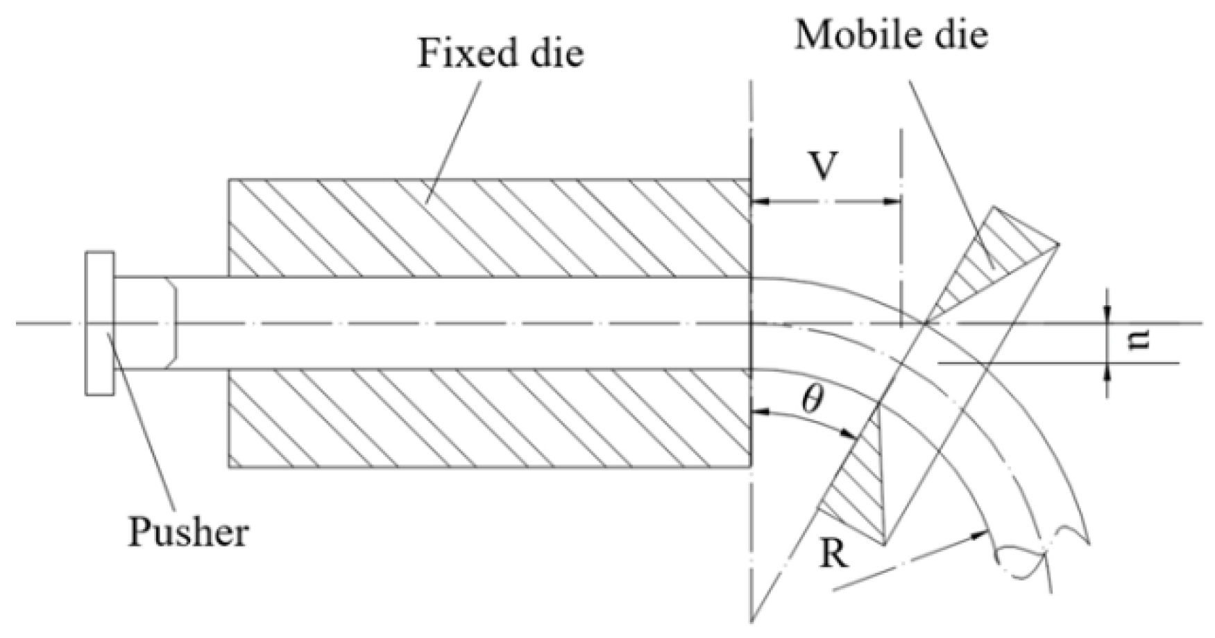
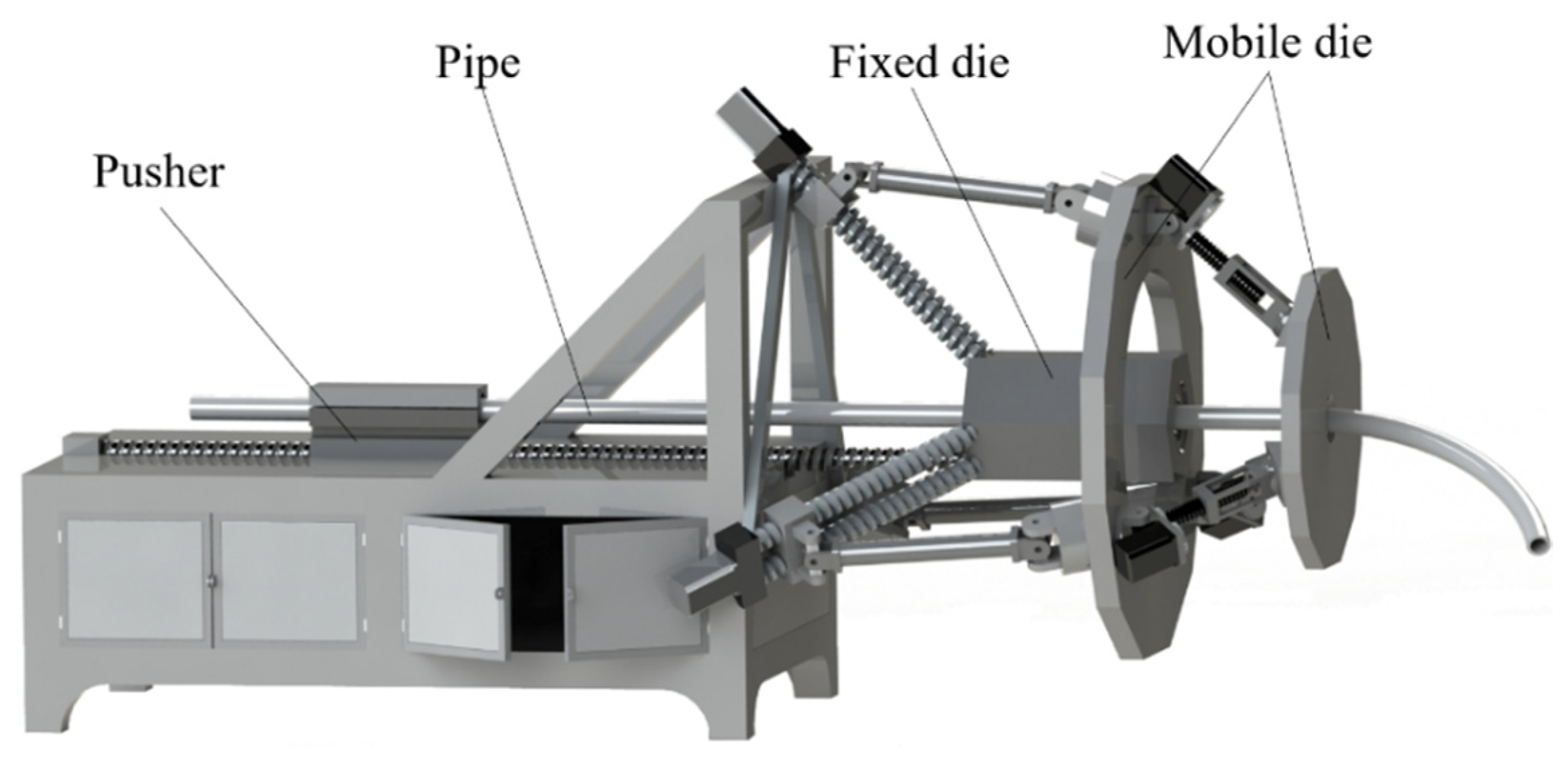
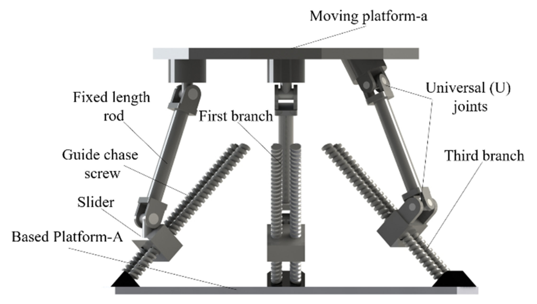
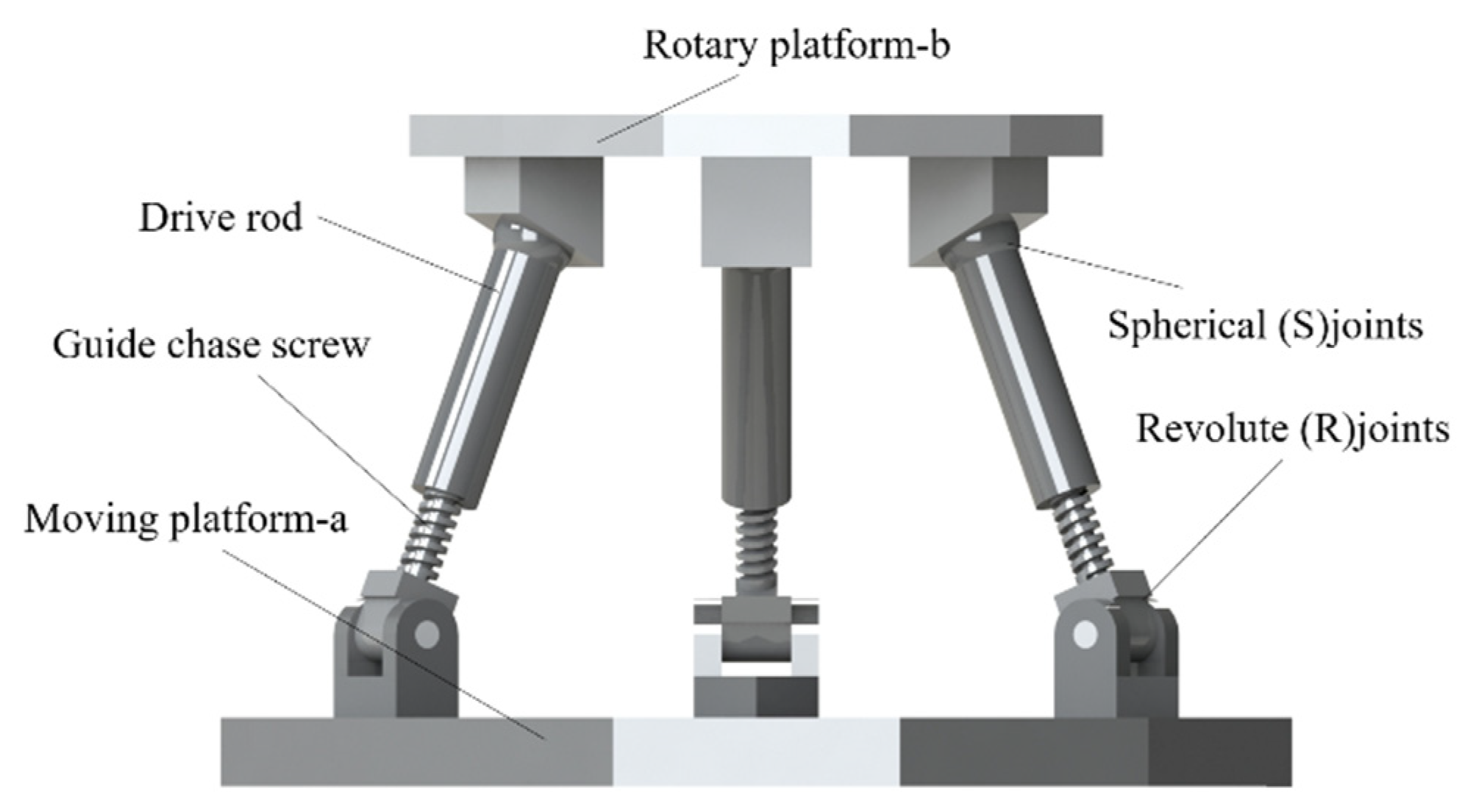
2. The Structural Design of Pipe-Bending Machine

The principle of spatial variable curvature bending forming is shown in Figure 1. This process consists of a fixed die, a mobile die, and a pusher [27,28]. The fixed die acts as a fixed pipe and guide. The mobile die can move and rotate in space and is the main part of this machine. The role of the pusher is feeding pipe. Each parameter is presented in Figure 1 and Table 1. The relationship among parameters is as seen in Equation (1). By this equation, it is found that the bending radius R of the pipe is related to V and u (detailed explanations of these parameters are given in Table 1). The rotation angle of mobile die θ is only for the purpose that the thrust of the mobile die to the pipe is perpendicular to the pipe.
{ R = u 2 + V 2 2 u = u 2 + V 2 2 u θ = arcsin V R
By understanding the principle of spatial variable curvature-bending forming, it is found that the most important part of the pipe-bending machine is the mobile die, which can do the translation and rotation motions in space. A new type of pipe-bending construction is presented in this paper, as is shown in Figure 2. The mobile die of this machine is a kind of 3PUU–3RPS structure. The device is mainly composed of a mounting frame, a pusher, a fixed die, and a mobile die. The mobile die is composed of a 3PUU moving part and a 3RPS rotary part, as shown in Figure 3 and Figure 4.

The Analysis on Degree of Freedom

The 3PUU moving part proposed in this article has three parallel branched chains which are asymmetrically distributed in space. Each connecting chain is composed of prismatic (P), lower universal, and upper universal joints arranged from the base to the output link. In the first two branches, the axis of the first revolute joint of lower universal (U) joints is perpendicular to the based platform-A, whereas the axis of the second revolute joints of the upper U joint is perpendicular to the moving platform-a. In the third branch, the axis of the first revolute joint of the lower U joint is parallel to the based platform-A, and the axis of the second revolute joints of upper U joint is parallel to the moving platform-a, as is shown in Figure 3.
For the first branched chain, the coordinate system is established as shown in Figure 5. The X -axis and Z -axis are along the two axes of the U joints; the Y -axis is perpendicular to the crosshead plane of the U joints. Therefore, in the initial assembly position, the screw system of the branch chain can be written as follows:
{ 1 = ( 0 0 0 ; 0 e 1 f 1 ) 2 = ( 0 0 1 0 0 0 ) 3 = ( 1 0 0 ; 0 0 0 ) 4 = ( 1 0 0 ; 0 e 4 f 4 ) 5 = ( 0 0 1 d 5 0 0 ) .
To calculate the reciprocal screw of five kinematic screws, all the variables in Equation (2) are imported into the formula r i = 0 , ( i = 1 , 2 , 3 ) , and the constraint screw of the single branched chain can be obtained as follows:
1 r = ( 0 0 0 ; 0 1 0 ) .
For the third branched chain, the coordinate system is established as shown in Figure 6. The X -axis and Y -axis are along the two axes of the U joints; the Z -axis is perpendicular to the crosshead plane of the U joints. Therefore, in the initial assembly position, the screw system of branch chain can be written as follows:
{ 1 = ( 0 0 0 ; 0 e 1 f 1 ) 2 = ( 1 0 0 ; 0 0 0 ) 3 = ( 0 1 0 ; 0 0 0 ) 4 = ( 0 1 0 ; d 4 0 0 ) 5 = ( 1 0 0 ; 0 e 5 0 ) .
To calculate the reciprocal screw of five kinematic screws, all the variables in Equation (4) are imported into the formula r i = 0 , ( i = 1 , 2 , 3 ) , and the constraint screw of the single branched chain can be obtained as follows:
3 r = ( 0 0 0 ; 0 0 1 ) .
In Equations (3) and (5), the first three elements of the constraint spiral are all zero. Thus, these two constraint screws are both constraint couples and perpendicular to the crosshead plane of the respective U joints. The second constraint screw is the same as the first one. Because three couples of branched chains are not parallel and linearly independent of each other, three independent constraints act on the moving platform-a. These three constrained couples constrain three rotational degrees of freedom, and the mobile platform has only three translational degrees of freedom. Therefore, the mobile platform can move along the X -axis, Y -axis, Z -axis and the directions of any linear combination of them.
The 3RPS rotary part has three parallel branched chains which are symmetrically distributed in space, as shown in Figure 4. Each connecting chain is composed of revolute (R), prismatic (P), and spherical (S) joints. For the first branched chain, the coordinate system is established (Figure 7). The origin is the first kinematic pair. The X -axis is along the axis of this revolute (R) joint, and the Z -axis is perpendicular to the based plane. Thus, the screw system of branch chain can be written as follows:
{ 1 = ( 1 0 0 ; 0 0 0 ) 2 = ( 0 0 0 ; 0 e f ) 3 = ( 1 0 0 ; 0 f e ) 4 = ( 0 1 0 ; f 0 0 ) 5 = ( 0 0 1 ; e 0 0 ) .
In the same way, the constraint screw of the single branched chain can be obtained as follows:
r = ( 1 0 0 ; 0 f e ) .
For the 3RPS rotary part, the three chains have a similar constraining force. This force can be applied on the rotary platform-b, located on the center of respective branched chain’s sphere joint and parallel to the axis of revolute joint. These three constraining forces are linearly independent and limited to three freedom degrees of the rotary platform-b. Through the analysis, the limited degrees of freedom include two translational degrees and one rotational degree. Thus, the rotary platform can only have a two-dimensional rotation in the plane and a translation along the Z -axis.
Through analysis, the 3PUU-3RPS mobile die has six degrees of freedom in total. The degree of freedom normally can also be calculated by using Equation (8). With the obtained results M = 6, the determined degree of freedom can be regarded as consistent with the theoretical obtained results, which also confirms the accuracy of analysis of 3PUU-3RPS system:
M = d ( n g 1 ) + i = 1 g f i + v = 6 × ( 15 18 1 ) + 30 + 0 = 6 .

3. Kinematic Analysis

Considering the independence between the 3PUU moving part and the 3RPS rotary part in the 3PUU-3RPS, in coming sections these two parts can be studied and analyzed respectively.

3.1. Inverse Position Model

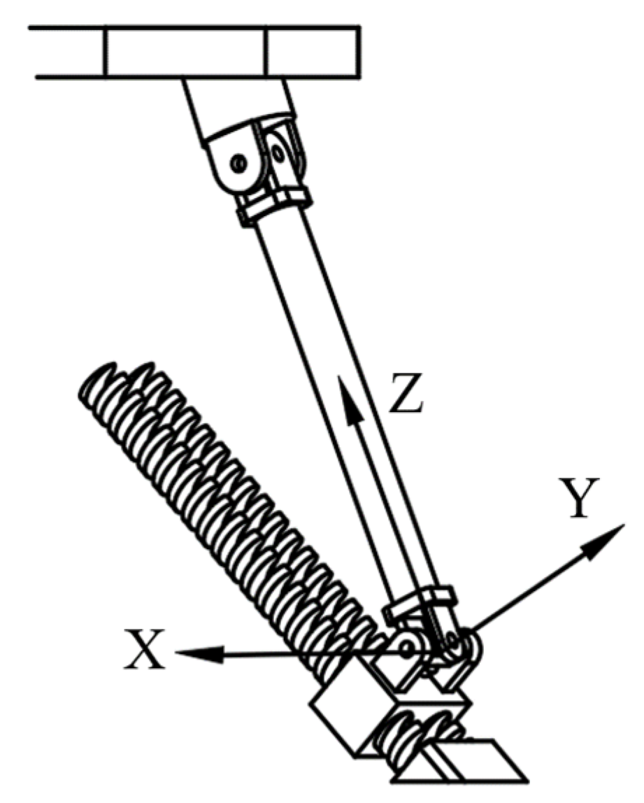
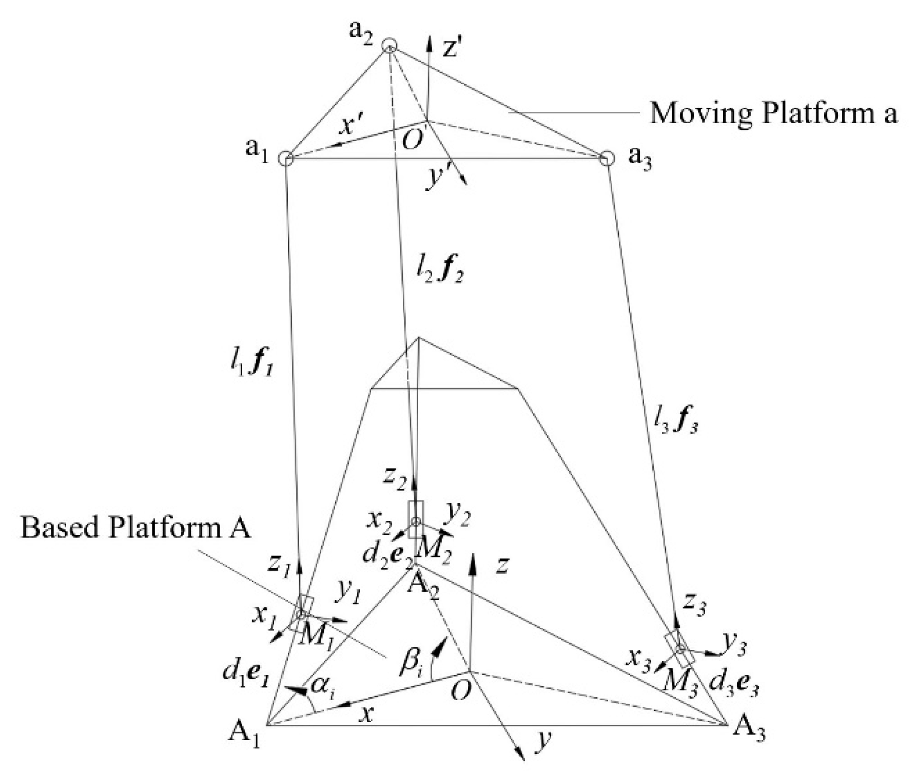
3.1.1. Inverse Position Model of 3PUU Moving Part

As shown in Figure 8, the based coordinate system is given. In the initial position, the moving coordinate system o x y z coincides with the based coordinate system o x y z . The direction from the origin O to O can be represented by a vector P , and the direction cosine matrix R is represented by Euler angles as is Equation (9), and C ϕ , C θ , C ψ , S ϕ , S θ , S ψ represent cos ϕ , cos θ , cos ψ , sin ϕ , sin θ , sin ψ , respectively.
R o o = [ C ϕ C θ C ψ S ϕ S ψ C ϕ C θ S ψ S ϕ C ψ C ϕ S θ S ϕ C θ C ψ + C ϕ S ψ S ϕ C θ C ψ + C ϕ S ψ S ϕ S θ S θ C ψ S θ S ψ C θ ]
Through the analysis of the degree of freedom, it is found that the 3PUU moving part only has three translational degrees of freedom, which induces ϕ = θ = ψ = 0 . Thus, the homogeneous transfer matrix T o o of the moving platform relative to the based platform can be written as follows:
T o o = [ 1 0 0 Δ x 0 1 0 Δ y 0 0 1 Δ z 0 0 0 1 ] ,
where Δ x ,   Δ y , and Δ z represent the moving distances of the platform a relative to the based platform-A along three directions of the x -axis, y -axis, and z -axis, respectively.
To conveniently describe the posture of each branch, a moving coordinate system M i x i y i z i is established at the center of the U joints which connect the slider and the fixed-length rod, where i represents the connecting chain number ( i = 1, 2, 3). The z -axis of the coordinate system is along the direction of the fixed-length rod. The y -axis is determined by the right-hand rule with the z -axis and the z i -axis. The direction cosine matrix M i o R of the coordinate system relative to the based coordinate system can be written as Equation (11), and the position of the fixed rod in the based coordinate system can be expressed by Equation (12):
M i o R = [ C ϕ i C θ i S ϕ i C ϕ i S θ i S ϕ i C θ i C ϕ i S ϕ i S θ i S θ i 0 C θ i ]
l i = R M i O l M i = R M i O [ 0 0 l ] = [ l C ϕ i S θ i l S ϕ i S θ i l C ϕ i ] ,   ( i = 1 , 2 , 3 ) ,
where P represents the position where the center of the moving platform o in based coordinate system, A i and   a i represent the position coordinate of point A i and   a i in the based coordinate system, a o i represents the position where point a i in the moving coordinate system o x y z , R represents the radius of platform-A, r represents the radius of platform-a, d i represents the translational distance of the slider, vector e i represents the unit vector that position of the screw in based coordinate system, l i represents the position of the fixed-length rod in the based coordinate system, l M i represents the position of the fixed-length rod in the moving coordinate system M i x i y i z i , M i represents the position of point M i in the based coordinate system. Through geometrical relation, Equations (13)–(18) can be obtained. Based these formulas, the translational distance of the slider d i can be calculated by mathematical methods, as Equation (19):
a o i = [ r cos β i r sin β i 0 ] ,   ( i = 1 , 2 , 3 )
A i = [ R cos β i R sin β i 0 ] ,   ( i = 1 , 2 , 3 )
e i = [ cos α cos β i cos α sin β i sin α ] ,   ( i = 1 , 2 , 3 )
M i = A i + d i e i ,   ( i = 1 , 2 , 3 )
l i = α i M i = α i A i d i e i ,   ( i = 1 , 2 , 3 )
a i = T o o a o i ,   ( i = 1 , 2 , 3 )
d i = ( a i T A i T ) e i + [ ( a i T A i T ) e i ] 2 α i A i 2 + l i 2 ,   ( i = 1 , 2 , 3 ) .

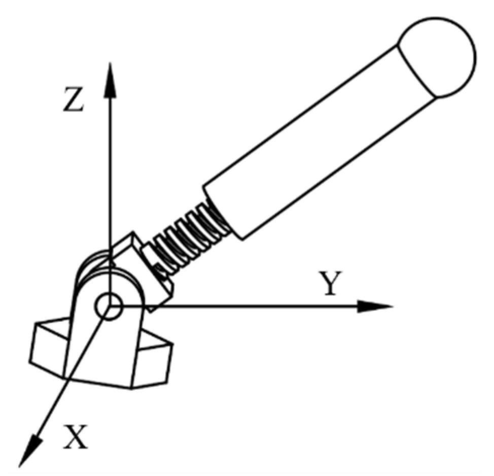
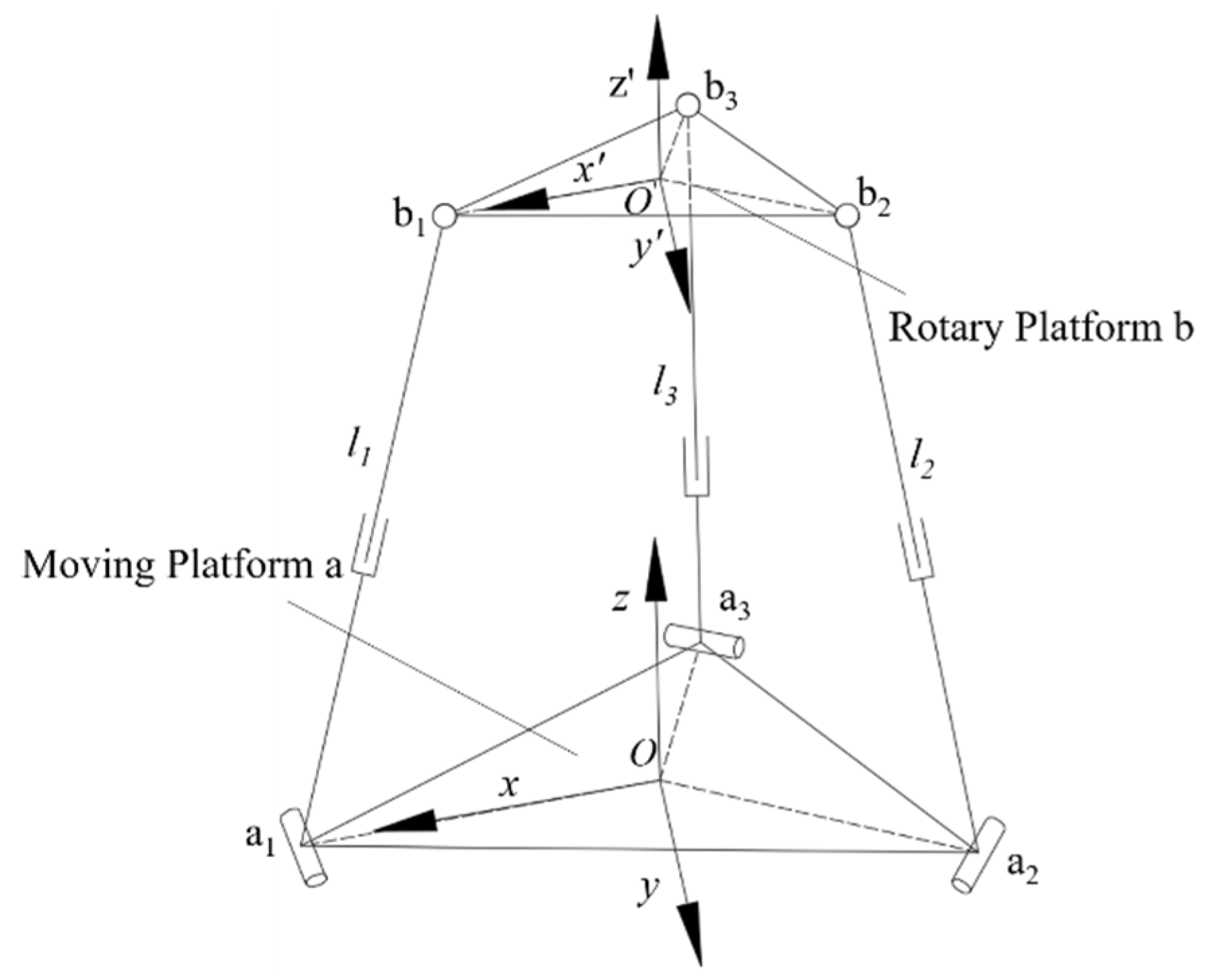
3.1.2. Inverse Position Model of 3RPS Rotary Part

As shown in Figure 9, the x -axis of the based coordinate system points to a 1 , the z -axis is perpendicular to the moving platform-a. The x -axis of the moving coordinate system points to b 1 , the z -axis is perpendicular to the rotary platform-b. In the initial position, the moving coordinate system o x y z coincides with the based coordinate system o x y z . The homogeneous transfer matrix T o o of the rotary platform b relative to the moving platform-a can be given as Equation (20). The position of the kinematic pair b i in the based coordinate system can be shown as Equation (21):
T o o = [ C ϕ C θ C ψ S ϕ S ψ C ϕ C θ S ψ S ϕ C ψ C ϕ S θ Δ x S ϕ C θ C ψ + C ϕ S ψ S ϕ C θ C ψ + C ϕ S ψ S ϕ S θ Δ y S θ C ψ S θ S ψ C θ Δ z 0 0 0 1 ]
b i = T o o b i , ( i = 1 , 2 , 3 ) .
By geometrical relationship, the coordinate values of point a i and   b i can be obtained easily in their respective coordinate systems. Through Equation (21), the coordinate values of the hinge point of the platform-b in the based coordinate system can be obtained. The position vector l i of the drive rod in the based coordinate system can be calculated by Equation (22), and the equation of the inverse position model can be expressed by Equation (23):
l i = b i a i = [ l i x l i y l i z ] T , ( i = 1 , 2 , 3 )
l i = l i x 2 + l i y 2 + l i z 2 , ( i = 1 , 2 , 3 ) .

3.2. Inverse Velocity Model and the Inverse Acceleration Model

3.2.1. The Inverse Velocity Model and the Inverse Acceleration Model of 3PUU Moving Part

By geometrical relationship, the position vector P of the center of platform-a can be written by Equation (24). Taking a derivative with respect to time for two sides of Equation (24), the velocity v of the center of the platform-a can be obtained by Equation (25), where ω represents the angular velocity of the platform-a and ω i represents the angular velocity of the fixed-length rod:
P = A i + d i e i + l i α i ,   ( i = 1 , 2 , 3 )
v = d i e i + ω i × l i ω × α i ,   ( i = 1 , 2 , 3 ) .
Calculate the dot product with the directional unit vector of the fixed-length rod f i for two sides of Equation (25), and through mathematical calculation, the translational speed d of the slider can be obtained by Equation (26). The matrix equation of Equation (26) can be expressed as Equation (27):
d i = f i T f i T e i v ,   ( i = 1 , 2 , 3 )
d = J 1 X .
In Equation (27), X represents the translational speed of the moving platform-a, and J 1 represents the velocity Jacobian matrix. They can be expressed as follows:
{ d = ( d 1 d 2 d 3 ) T X = ( v x v y v z ) T
J 1 = [ f 1 T f 1 T e 1 f 2 T f 2 T e 2 f 3 T f 3 T e 3 ] T .
To establish the inverse acceleration model, first take a derivative with respect to time for the two sides of Equation (26), as Equation (30). Calculate the dot product with a directional unit vector of the fixed-length rod f i for two sides of Equation (30), and through mathematical calculation, the translational acceleration d of the slider can be obtained by Equation (31). The matrix equation of Equation (31) can be expressed as Equation (32):
v = d i e i + ω i × l i + ω i × ( ω i × l i ) ,   ( i = 1 , 2 , 3 )
d i = f i T f i T e i v f i T f i T e i ω i × ( ω i × l i ) ,   ( i = 1 , 2 , 3 )
d = J 1 X + K 1 ,
where, X represents the translational acceleration of the moving platform-a, K 1 represents the second order kinematic influence coefficient. They can be expressed as follows:
{ d = ( d 1 d 2 d 3 ) T X = ( a x a y a z ) T
J 1 = [ f 1 T f 1 T e 1 f 2 T f 2 T e 2 f 3 T f 3 T e 3 ] , K 1 = [ f 1 T f 1 T e 1 ω 1 × ( ω 1 × l 1 ) f 2 T f 2 T e 2 ω 2 × ( ω 2 × l 2 ) f 3 T f 3 T e 3 ω 3 × ( ω 3 × l 3 ) ] .
As above, the inverse velocity model of the 3PUU moving part is expressed by Equation (27), and the inverse acceleration model is expressed by Equation (32).

3.2.2. Inverse Velocity and Acceleration Models of 3RPS Rotary Part

By mathematical relationship, Equation (35) can be achieved, where l i represents the relationship between two hinges of the branched chain. Through mathematical calculation, the velocity of the drive rod l i can be obtained by Equations (36) and (37), where v b i represents the velocity vector of the hinge point b i :
l i 2 = l i l i , ( i = 1 , 2 , 3 )
l i = Q i v b i , ( i = 1 , 2 , 3 )
Q i = l i l i , ( i = 1 , 2 , 3 ) .
The velocity vector of the hinge point b i of the platform-b can also be obtained through the Equation (38), where ω = [ ω x ω y ω z ] T represents the angular velocity of platform-b, v = [ v x v y v z ] T represents the velocity of the center of platform-b, r b i represents the position vector of hinge point in the moving coordinate system:
v b i = v + ω × r b i , ( i = 1 , 2 , 3 ) .
Considering v x = v y = ω z = 0 , the velocity P of the rotary platform-b can be obtained by Equation (39). By mathematical calculation, the velocity l i of the branched chain can be calculated as Equation (40):
P = [ ω x ω y v z ] T
{ l i = Q i v b i = Q i G b i P G b i = [ i × r b i j × r b i k ]   ,                     ( i = 1 , 2 , 3 ) .
The matrix equation of Equation (40) can be expressed by Equation (41), where q represents the translational speed of the drive rod, P represents the translational speed of the rotary platform-b, J 2 represents the velocity Jacobian matrix of 3RPS rotary part. They can be expressed as follows:
q = J 2 P ,
where q and J 2 can be expressed as follows:
q = [ l 1 l 2 l 3 ]
J 2 = [ Q 1 G b 1 Q 2 G b 2 Q 3 G b 3 ] T
By taking the derivation with respect to time for the two sides of Equation (40), and through mathematical calculation, the acceleration of the drive rod l i can be obtained as Equation (44), where A b i represents the acceleration of the hinge point b i of rotary platform-b:
l i = Q i A b i + v b i v b i l i 2 l i , ( i = 1 , 2 , 3 ) .
The acceleration of the hinge point A b i can also be expressed by Equation (45), where ε = ( ε x ε y ε z ) T represents the angular acceleration of rotary platform-b and A = ( A x A y A z ) T represents the acceleration of the center of the rotary platform-b:
A b i = A + ε × r b i + ω × ( ω × r b i ) , ( i = 1 , 2 , 3 ) .
Due to A x = A y = ε z = 0 in this mechanism, the acceleration A b i of the hinge point b i can be expressed as Equation (46), where P is the acceleration of the rotary platform-b, H b i can be expressed as Equation (47). Through mathematical calculation, the acceleration l i can be achieved, as Equation (48):
{ A b i = G b i P + P T H b i P P = [ ε x ε y A z ] T           ,                         ( i = 1 , 2 , 3 )
H b i = [ i × ( i × r b i ) j × ( i × r b i ) 0 i × ( j × r b i ) j × ( j × r b i ) 0 0 0 0 ]
l i = Q i T G b i P + P T [ Q i T H b i + 1 l i ( G b i T G b i G b i Q i Q i T G b i ) ] P ( i = 1 , 2 , 3 ) .
The matrix equation of Equation (48) can be expressed by Equation (49), and q represents the acceleration of the drive rod, P represents the acceleration of the rotary platform-b, J 2 represents the velocity Jacobian matrix of 3RPS rotary part, and K 2 represents the second order kinematic influence coefficient of 3RPS rotary part. They can be expressed as follows:
{ q = J 2 P + P T K 2 P q = [ l 1 l 2 l 3 ] T K 2 m : n = { [ U 1 ] m : n [ U 2 ] m : n [ U 3 ] m : n } [ U i ] = Q i T H b i + 1 l i { G b i T G b i G b i Q i Q i T G b i } .
As above, the inverse velocity model of the 3RPS rotary part is expressed by Equation (41), and the inverse acceleration model is expressed by Equation (49).

4. Analysis of Numerical Simulation Result

The geometric parameters of the 3PUU-3RPS mobile die is shown in Table 2. R represents the radius of the based platform-a, r represents the radius of the moving platform-a, s represents the radius of the rotary platform-b, l represents the length of the fixed-length rod, and α represents the angle of inclination of the screw in 3PUU moving part.

4.1. Kinematics Simulation and Calculation Based on ADAMS and MATLAB

In this section, the kinematics simulation was accomplished in ADAMS (Automatic Dynamic Analysis of Mechanical Systems, Newport Beach, CA, USA). At the same time, combined with MATLAB software (Matrix&Laboratory, Dubai, U.A.E), some simulation results and the relevant theoretical analysis results were compared to verify the reliability of the proposed analytic model.
Kinematics simulation is the process of finding the inverse model, that is, giving the output, and then solving the displacement, velocity, and acceleration of each branch. First, a 3D model was built through SolidWorks (Massachusetts, USA). Then, the model was imported into ADAMS, and the constraint of the kinematic pair was added. Finally, a driving force was applied to the end-effector.
Taking the fixed coordinate system o x y z as the reference system, the motion parameters of the moving platform-a of the 3UPU parallel mechanism can be shown as Equation (50), and the motion parameters of the rotary platform-b of the 3RPS parallel mechanism is as Equation (51). Figure 10 and Figure 11 compare the simulation results with analysis results by the displacement curve, velocity curve, and acceleration curve of each branched chain. The analysis model was validated by the comparison of the simulation results with the calculation results.
{ x = 0.35 × sin ( 5 × t ) y = 0.35 × cos ( 5 × t ) z = 0
{ ϕ = 0.5 × cos ( 5 × t ) θ = 0.5 × sin ( 5 × t ) z = 0 ,
where x ,   y , and   z represent the move function along x -axis, y -axis, and z -axis, respectively and ϕ and θ represent the rotational functions along x -axis and y -axis, respectively.

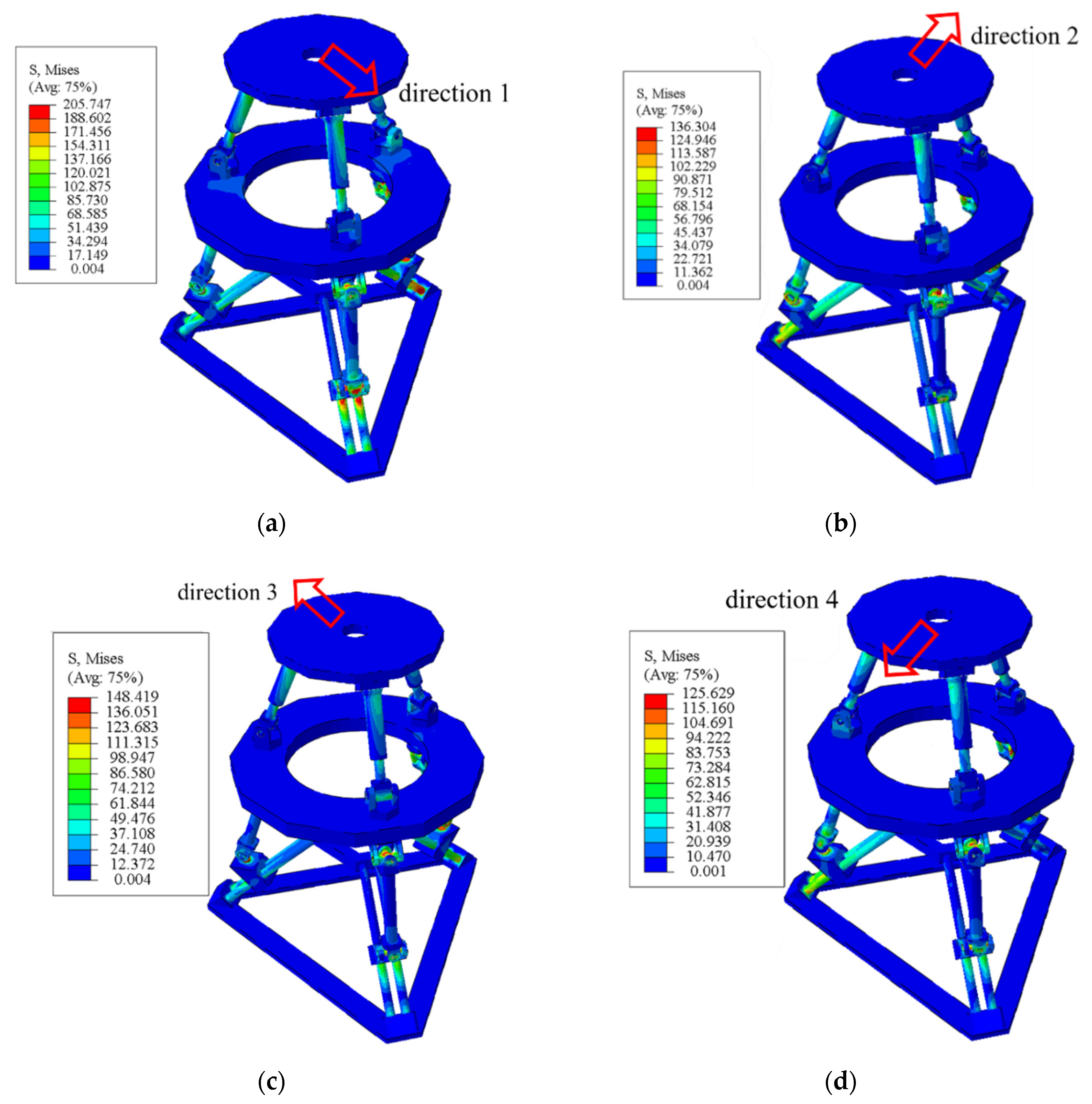
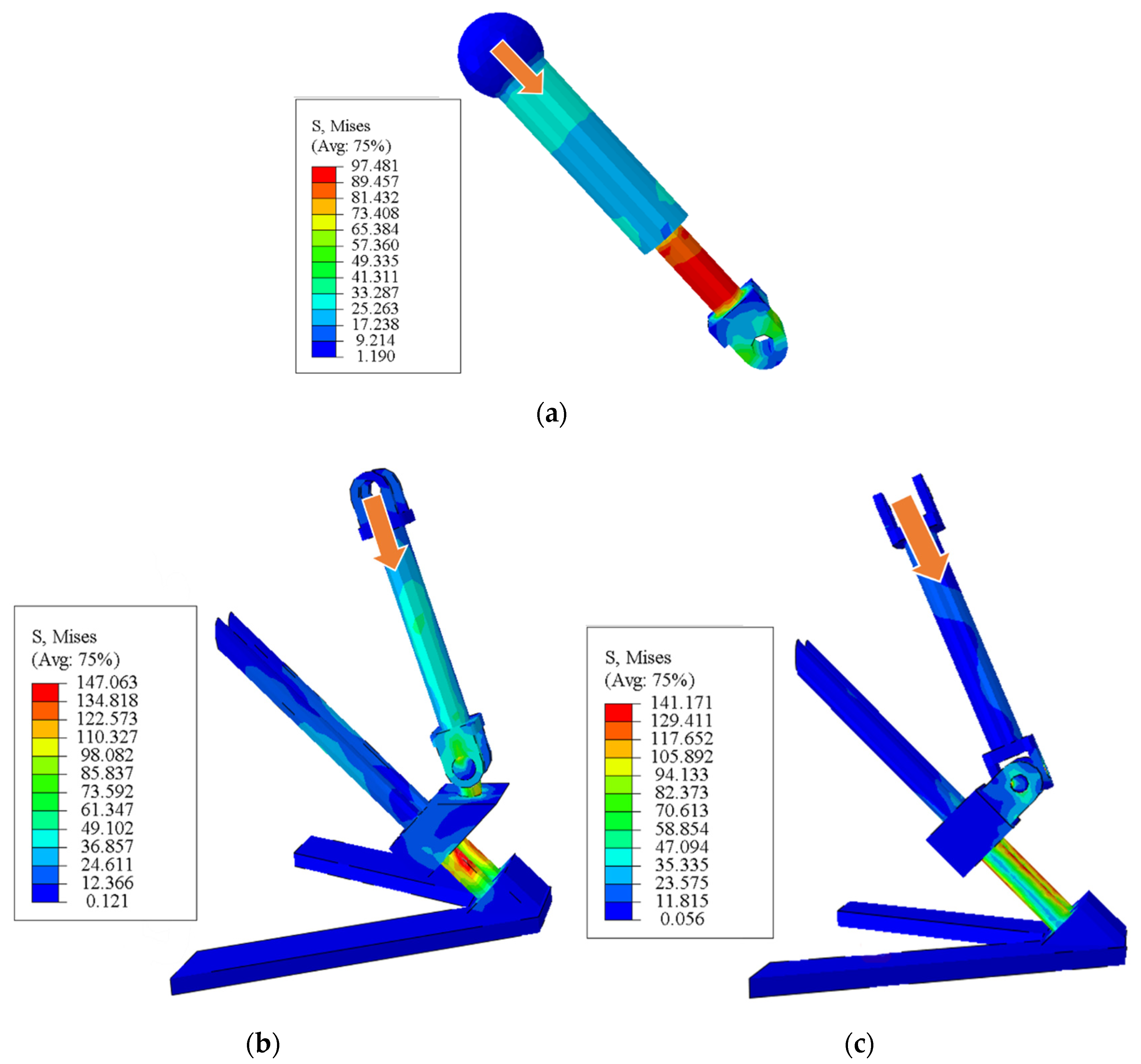
4.2. Static Stiffness Analysis

During the forming process, the hybrid mechanism normally results in the stress concentration and poor structural stiffness easily. Furthermore, it may affect the dynamic property and positioning accuracy of the mechanism, and even cause mechanical damage. Thus, it is necessary to carry out the static analysis to verify the stress distribution and structural deformation of each component and joint, and also improve and optimize the structural configuration and the rationality.
In this section, finite element simulation software ABAQUS (Paris, France) is used to analyze the stiffness of the whole structure and its branch chains. The geometric models were created and assembled in Solidworks, and then imported into ABAQUS. The FE model is shown in Figure 12 which includes the based platform, moving platform, rotary platform, PUU structure, and RPS structure. The based platform, moving platform, and rotary platform were defined as rigid bodies. The PUU and RPS structures were defined as deformable bodies which were given the material properties of tool steel Cr12Mo1V1, and its specific parameters are given in Table 3. These deformable bodies were meshed by using C3D4 solid elements which were four-node linear tetrahedron elements, and the minimum element size was 1 mm. The interaction was set to general contact, where the slider in the 3PUU structure was tied to the lead screw on the based platform. Because moving parts of the structure are lubricated in practice, the coefficient of friction was identified as 0.1. The analysis step was identified as static general. In addition, the base platform was completely fixed, the mobility and rotation degrees of the 3PUU and 3RPS branch chains were preserved. Through the bending test of an aluminum alloy tube with diameter of 30 mm and wall thickness of 2 mm by using a universal testing machine, it is found that the bending force of the tube is 5 kN [29]. In order to verify the stability and rationality of the designed mechanism, 15 kN force was used to simulate the mechanism. So a static load of 15 kN was applied to the center of the rotary platform-b along four directions as shown in Figure 13. The stress distribution is also shown in Figure 13. The static analysis of each branch chain was also carried out. In addition, the static loads of 8 kN were applied, and the stress distribution was as shown in Figure 14.
By investigating the whole stress distribution, the maximum stress can be found located at the U-joint of the PUU structure. On the branch chain stress distribution, the maximum stress is located at the lower link of the branch chain. The maximum stress value is 205 MPa, which is far less than the yield strength of tool steel Cr12Mo1V1. It is proved that static stiffness can meet the requirements and the structure design is reasonable.

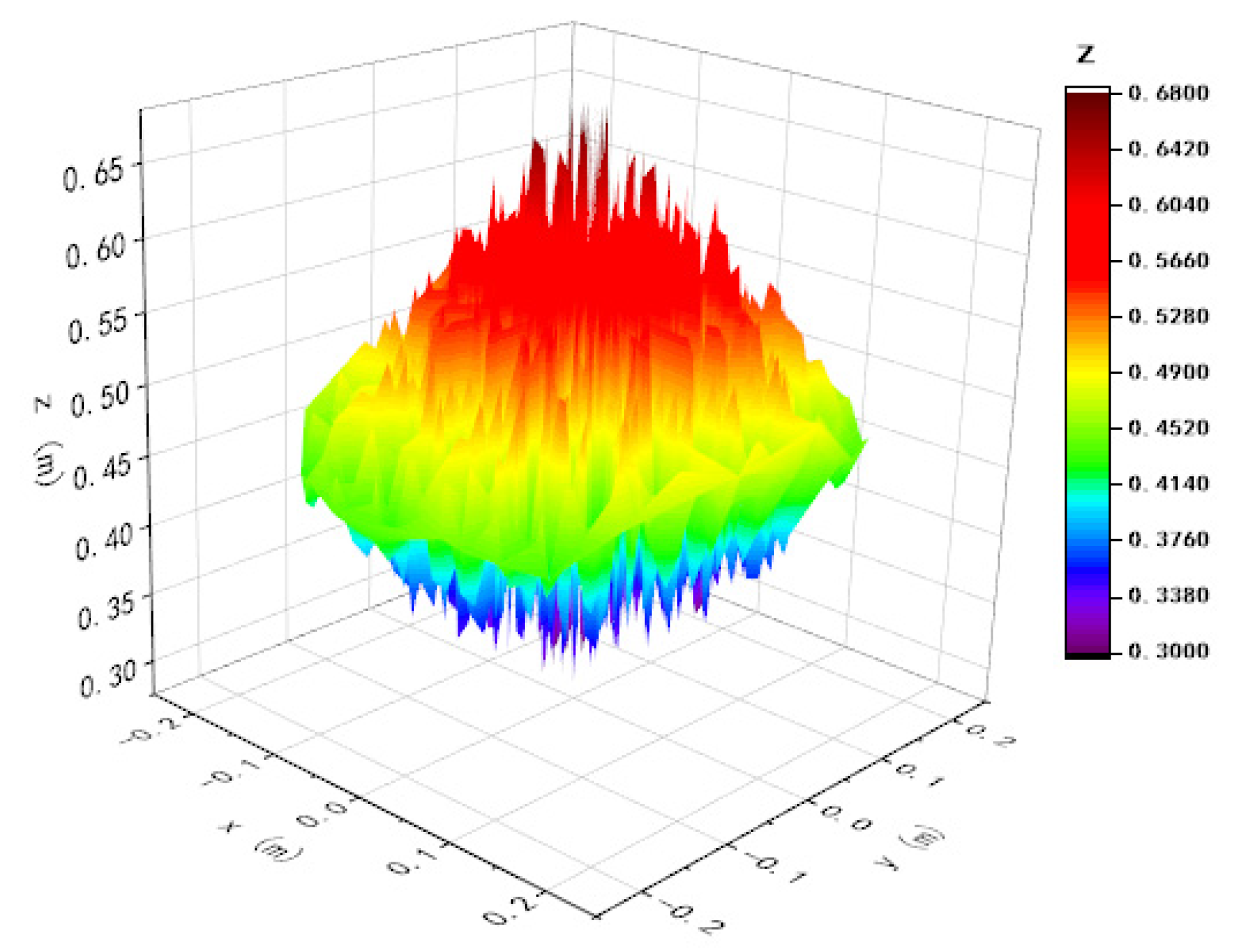
4.3. Analysis of Workspace

The main factors on the working space of the parallel mechanism are the length of the rod, the angle of rotation of the kinematic pair and the interference of the connecting rods [30]. The limitation about the length of the rod, the translational distance of each slider, and the length of each drive rod must satisfy Equation (52) for this 3PUU-3RPS mobile die:
{ 0 d i d max 0 l i l max ,                         ( i = 1 ,     2 ,     3 ) .
The limitation about the angle of rotation of the kinematic pair of the 3PUU-3RPS mobile die must satisfy Equation (53). Through Equation (12), the angles of rotation ϕ M i and θ M i can be achieved by Equation (54). By geometrical relationship, the angles of rotation ϕ a i and θ a i can be achieved by Equation (55):
{ 0 ϕ a i ϕ M a x 0 θ a i θ M a x 0 ϕ M i ϕ M a x 0 θ M i θ M a x 0 θ B i θ B M a x 0 θ b i θ b M a x , ( i = 1 , 2 , 3 )
{ ϕ M i = arccos l i z l θ M i = arcsin l i x l i z
{ ϕ a i = ϕ M i θ a i = θ M i .
The angles of rotation θ B i and θ b i in the 3RPS rotary part can be calculated by Equation (56), where vector n b i represents the position vector of the base of spherical (S) joints:
{ θ b i = arccos l i ( T o o n b i ) | l i | θ B i = arccos l i B i | l i | | B i | , ( i = 1 , 2 , 3 ) .
For the 3PUU moving part, the maximum rotary angle of U joints is ± π / 4 , and the maximum translational distance of the slider is d max = 0.7 m. For the 3RPS rotary part, the maximum rotary angle of spherical (S) joints is ± π / 4 , the maximum translational distance of slider is l max = 0.5 m. Through the polar coordinate searching method, the workplace of this 3PUU-3RPS mobile die is calculated by using MATLAB and is shown in Figure 15. It is found that the range of the mechanism is 0.3 m in the Z direction, and the range of motion in the X and Y directions is ±0.2 m. Currently, the extreme structure of bending tubes is characterized by small bending radii (Rd/D < 3) [31]. According to the results of the previous FE simulation results by Equation (1), it is found that the bending die needs to move 55 mm when the minimum bending radii is 90 mm [32]. Therefore, Equation (1) describes the motion of tube bending that can be performed within the workspace presented in Figure 15.

5. Conclusions

In this research, a 3PUU-3RPS hybrid mechanism for the free-bending forming of tubes was presented. The rationality and reliability of the hybrid mechanism are verified by theoretical analysis and simulation. The mechanism can better serve the needs of production activities. The main results are as follows:
  • The degree of freedom of the proposed mechanism was analyzed based on the screw theory. It can meet the requirements of free-bending forming by combining the 3PUU moving part and 3RPS rotary part.
  • In aspects of kinematics, the inverse position model, inverse velocity model and inverse acceleration model were established based on structural characteristics of the 3PUU–3RPS mobile die. Furthermore, the kinematics simulation and static stiffness were accomplished. The corresponding numerical simulation and the relevant theoretical analysis were also conducted to verify the reliability and feasibility of the mechanism.
  • Based on the inverse position model, the working space of this mechanism and the relationship between end-effector and actuator was also presented.
To conclude, this study provides an in-depth understanding of the bending process of tubes by theoretical and simulation analyses. Moreover, the designed 6-DOF hybrid mechanism is appropriate for the spatial variable curvature tube-bending forming, which provides theoretical guidance for building a device to accomplish the free- bending forming of tubes. The next step, the experimental validation, will be carried out in future work.

Author Contributions

Simulation, formal analysis, investigation, writing and reviewing, S.Z. and Y.L.; Funding acquisition, Supervision, Writing—review & editing, Z.Y.; Conceptualization, Z.Z.; Methodology and supervision, L.S.; Validation and supervision, B.Y.; Resources, J.G. All authors have read and agreed to the published version of the manuscript.

Funding

This work was supported by the National Natural Science Foundation of China (No. 51975327 and 52175337).

Institutional Review Board Statement

Not applicable.

Informed Consent Statement

Not applicable.

Data Availability Statement

Not applicable.

Conflicts of Interest

The authors declare no conflict of interest.

References

  1. Song, F.; Yang, H.; Li, H.; Zhan, M.; Li, G. Springback prediction of thick-walled high-strength titanium tube bending. Chin. J. Aeronaut. 2013, 26, 1336–1345. [Google Scholar] [CrossRef]
  2. Wu, J.; Zhang, Z.; Shang, Q.; Li, F.; Hui, Y.; Fan, H. A method for investigating the springback behavior of 3D tubes. Int. J. Mech. Sci. 2017, 131, 191–204. [Google Scholar] [CrossRef]
  3. Zhou, W.; Shao, Z.; Yu, J.; Lin, J. Advances and Trends in Forming Curved Extrusion Profiles. Materials 2021, 14, 1603. [Google Scholar] [CrossRef] [PubMed]
  4. Li, H.; Ma, J.; Liu, B.Y.; Gu, R.J.; Li, G.J. An insight into neutral layer shifting in tube bending. Int. J. Mach. Tools Manuf. 2018, 126, 51–70. [Google Scholar] [CrossRef]
  5. Wu, J.; Zhang, Z. An improved procedure for manufacture of 3D tubes with springback concerned in flexible bending process. Chin. J. Aeronaut. 2021, 34, 267–276. [Google Scholar] [CrossRef]
  6. Ma, J.; Li, H.; Fu, M.W. Modelling of Springback in Tube Bending: A Generalized Analytical Approach. Int. J. Mech. Sci. 2021, 204, 106516. [Google Scholar] [CrossRef]
  7. Yang, H.; Li, H.; Ma, J.; Li, G.; Huang, D. Breaking bending limit of difficult-to-form titanium tubes by differential heating-based reconstruction of neutral layer shifting. Int. J. Mach. Tools Manuf. 2021, 166, 103742. [Google Scholar] [CrossRef]
  8. Zhan, M.; Yang, H.; Huang, L.; Gu, R. Springback analysis of numerical control bending of thin-walled tube using numerical-analytic method. J. Mater. Processing Technol. 2006, 177, 197–201. [Google Scholar] [CrossRef]
  9. Gu, R.J.; Yang, H.; Zhan, M.; Li, H.; Li, H.W. Research on the springback of thin-walled tube NC bending based on the numerical simulation of the whole process. Comput. Mater. Sci. 2008, 42, 537–549. [Google Scholar] [CrossRef]
  10. Yang, H.; Li, H.; Zhang, Z.; Zhan, M.; Liu, J.; Li, G. Advances and Trends on Tube Bending Forming Technologies. Chin. J. Aeronaut. 2012, 25, 1–12. [Google Scholar] [CrossRef]
  11. Wagoner, R.H.; Lim, H.; Lee, M.-G. Advanced Issues in springback. Int. J. Plast. 2013, 45, 3–20. [Google Scholar] [CrossRef]
  12. Ma, J.; Welo, T. Analytical springback assessment in flexible stretch bending of complex shapes. Int. J. Mach. Tools Manuf. 2021, 160, 103653. [Google Scholar] [CrossRef]
  13. Staupendahl, D.; Chatti, S.; Tekkaya, A.E. Closed-loop control concept for kinematic 3D-profile bending. AIP Conf. Proc. 2016, 1769, 150002. [Google Scholar]
  14. Yang, D.Y.; Bambach, M.; Cao, J.; Duflou, J.R.; Groche, P.; Kuboki, T.; Sterzing, A.; Tekkaya, A.E.; Lee, C.W. Flexibility in metal forming. CIRP Ann. 2018, 67, 743–765. [Google Scholar] [CrossRef]
  15. Zhang, Z.K.; Wu, J.J.; Guo, R.C.; Wang, M.Z.; Li, F.F.; Guo, S.C.; Wang, Y.A.; Liu, W.P. A semi-analytical method for the springback prediction of thick-walled 3D tubes. Mater. Des. 2016, 99, 57–67. [Google Scholar] [CrossRef]
  16. Zhang, S.; Wu, J.; Wang, Q.; Liang, Z. Research on Springback in Tube Bending Process. Aeronaut. Manuf. Technol. 2014, 454, 45–50. [Google Scholar]
  17. Murata, M.; Kuboki, T. CNC tube forming method for manufacturing flexibly and 3-Dimensionally bent tubes. In 60 Excellent Inventions in Metal Forming; Tekkaya, A.E., Homberg, W., Brosius, A., Eds.; Springer: Berlin/Heidelberg, Germany, 2015; pp. 363–368. [Google Scholar]
  18. Plettke, R.; Vatter, P.H.; Vipavc, D. Basics of Process Design for 3D freeform bending. Steel Res. Int. 2012, S, 307–310. [Google Scholar]
  19. Gantner, P.; Bauer, H.; Harrison, D.K.; de Silva, A.K.M. Free-Bending—A new bending technique in the hydroforming process chain. J. Mater. Processing Technol. 2005, 167, 302–308. [Google Scholar] [CrossRef]
  20. Chatti, S.; Hermes, M.; Tekkaya, A.E.; Kleiner, M. The new TSS bending process: 3D bending of profiles with arbitrary cross-sections. CIRP Ann. 2010, 59, 315–318. [Google Scholar] [CrossRef]
  21. Becker, C.; Staupendahl, D.; Hermes, M.; Chatti, S.; Tekkaya, A.E. Incremental Tube Forming and Torque Superposed Spatial Bending—A View on Process Parameters. Steel Res. Int. 2012, S, 415–418. [Google Scholar]
  22. Hudovernik, M.; Kosel, F.; Staupendahl, D.; Tekkaya, A.; Kuzman, K. Application of the bending theory on square-hollow sections made from high-strength steel with a changing angle of the bending plane. J. Mater. Processing Technol. 2014, 214, 2505–2513. [Google Scholar] [CrossRef]
  23. Strano, M.; Colosimo, B.M.; Castillo, E.D. Improved design of a three roll tube bending process under geometrical uncertainties. AIP Conf. Proc. 2011, 1353, 35–40. [Google Scholar]
  24. Vatter, P.H.; Plettke, R. Process model for the design of bent 3-dimensional free-form geometries for the three-roll-push-bending process. Procedia CIRP 2013, 7, 240–245. [Google Scholar] [CrossRef]
  25. Goto, H.; Ichiryu, K.; Saito, H.; Ishikura, Y.; Tanaka, Y. Applications with a new 6-DOF bending machine in tube forming processes. In Proceedings of the JFPS International Symposium on Fluid Power, Toyama, Japan, 15–18 September 2008; The Japan Fluid Power System Society: Tokyo, Japan, 2008; pp. 183–188. [Google Scholar]
  26. Goto, H.; Tanaka, Y.; Ichiryu, K. 3D Tube Forming and Applications of a New Bending Machine with Hydraulic Parallel Kinematics. Int. J. Autom. Technol. 2012, 6, 509–515. [Google Scholar] [CrossRef]
  27. Kawasumi, S.; Takeda, Y.; Matsuura, D. Precise pipe-bending by 3-RPSR parallel mechanism considering springback and clearances at dies. Trans. Jpn. Soc. Mech. Eng. 2014, 80, 343. [Google Scholar]
  28. Takeda, Y.; Inada, S.; Kawasumi, S.; Matsuura, D.; Hirose, K.; Ichiryu, K. Kinematic design of 3-RPSR parallel mechanism for movable-die drive mechanism of pipe bender. Rom. J. Tech. Sci. Appl. Mech. 2013, 58, 71–96. [Google Scholar]
  29. Li, Y.; Li, A.; Yue, Z.; Qiu, L.; Badreddine, H.; Gao, J.; Wang, Y. Springback prediction of AL6061 pipe in free bending process based on finite element and analytic methods. Int. J. Adv. Manuf. Technol. 2020, 109, 1789–1799. [Google Scholar] [CrossRef]
  30. Xu, H.; Li, J.; Chen, Y.; Zhang, R.; Gao, J. Kinematic Modeling of Spherical Parallel Manipulator with Vectored Thrust Function for Underwater Robot Based on Screw Theory. Robot 2016, 38, 745–753. [Google Scholar]
  31. Li, H.; Yang, H.; Zhang, Z.Y.; Li, G.J.; Liu, N.; Welo, T. Multiple instability-constrained tube bending limits. J. Mater. Processing Technol. 2014, 214, 445–455. [Google Scholar] [CrossRef]
  32. Li, Y.; Yue, Z.; Min, X.; Gao, J. Simulation and optimization of the free bending process of aluminum alloy 6061 pipe. Chin. J. Eng. 2020, 42, 769–777. [Google Scholar]
Figure 1. Principle of spatial variable curvature bending forming.
Machines 10 00470 g001
Figure 2. Whole structural design for free bending device.
Machines 10 00470 g002
Figure 3. 3PUU moving part.
Machines 10 00470 g003
Figure 4. 3RPS rotary part.
Machines 10 00470 g004
Figure 5. Coordinate system of first branch chain of 3PUU moving part.
Machines 10 00470 g005
Figure 6. Coordinate system of third branch chain of 3PUU moving part.
Machines 10 00470 g006
Figure 7. Coordinate system of first branch chain of 3RPS rotary part.
Machines 10 00470 g007
Figure 8. Schematic diagram of 3PUU moving part.
Machines 10 00470 g008
Figure 9. Schematic diagram of 3RPS rotary part.
Machines 10 00470 g009
Figure 10. Displacement, velocity, and acceleration curves in the 3PUU moving part. (a) Displacement curves of each branched chain in 3PUU moving part; (b) velocity curves of each branched chain in 3PUU moving part; (c) acceleration curves of each branched chain in the 3PUU moving part.
Machines 10 00470 g010aMachines 10 00470 g010b
Figure 11. Length, velocity and acceleration curves in the 3RPS rotary part. (a) Length curve of each branched chain in 3RPS rotary part; (b) velocity curves of each branched chain in the 3RPS rotary part; (c) acceleration curves of each branched chain in the 3RPS rotary part.
Machines 10 00470 g011
Figure 12. FE modeling of 3PUU-3PRS.
Machines 10 00470 g012
Figure 13. Stress distribution along different directions. (a) Stress distribution along the direction-1; (b) stress distribution along the direction-2; (c) stress distribution along the direction-3; (d) stress distribution along the direction-4.
Machines 10 00470 g013
Figure 14. Stress distribution of branch chain. (a) Stress distribution of branch chain RPS; (b) stress distribution of PUU branch chain-1; (c) stress distribution of PUU branch chain-2.
Machines 10 00470 g014
Figure 15. Workplace of 3PUU-3RPS mobile die.
Machines 10 00470 g015
Table 1. Bending parameters of pipe.
RBending radius of the pipe
VDistance between the fixed die and the mobile die
uOffset between the center line of the fixed die and the center of the mobile die
θAngle of rotation of the mobile die
Table 2. The geometric parameters of 3PUU-3RPS mobile die.
R/mr/ms/ml/m α /rad
0.50.30.20.350.7
Table 3. Material parameters of tool steel Cr12Mo1V1.
Material PropertyValue
Poisson ratio0.269
Young’s modulus (MPa)206,000
Yield strength (MPa)430
Tensile strength (MPa)780
Density (kg/cm3)7.89
Publisher’s Note: MDPI stays neutral with regard to jurisdictional claims in published maps and institutional affiliations.

