Composite Fault Diagnosis of Rolling Bearing Based on Chaotic Honey Badger Algorithm Optimizing VMD and ELM

Abstract

In order to effectively extract the characteristic information of bearing vibration signals and improve the classification accuracy, a composite fault diagnosis method of rolling bearing based on the chaotic honey badger algorithm (CHBA), which optimizes variational mode decomposition (VMD) and extreme learning machine (ELM), is proposed in this paper. Firstly, aiming to solve the problem that the HBA optimization process can easily fall into local optimization and slow convergence speed, sinusoidal chaotic mapping is introduced to improve HBA, and the advantages of CHBA are verified by 23 benchmark functions. Then, taking the Gini index of the square envelope (GISE) as the fitness function, the VMD is optimized with CHBA to obtain the optimal number of modes K and the quadratic penalty factor. Secondly, the first four IMF components with the largest GISE values are selected, and the IMF components are grouped by the “Systematic Sampling Method (SSM)” to calculate the signal energy to form the fault feature vector. Finally, taking the classification error rate as the fitness function, the feature vector is input into the ELM model optimized by CHBA to classify and identify different types of faults. Through experimental analysis, and compared with BP, ELM, GWO-ELM, and HBA-ELM, this method has better diagnosis results for composite faults, and the accuracy of fault classification can reach 100%, which provides a new way to solve the problem of composite fault diagnosis.

1. Introduction

Rolling bearing is the core component of mechanical equipment and plays an irreplaceable role. It is known as the “joint of industry”. It is widely used in automobile, high-speed railway, wind power generation, chemical industry, shipbuilding, aerospace and other fields. However, due to its special structural design and harsh working environment, it often fails, resulting in safety accidents and economic losses. According to statistics, mechanical equipment failure caused by bearing failure accounts for about 1/3 of the total number of damages. Therefore, the advanced fault diagnosis method is of great significance for the safe operation of the equipment. There are two common fault diagnosis methods: model-based and data-driven [1]. Firstly, the signals of the bearing are collected by sensors, and then the collected signals are analyzed and processed to identify the fault type and damage degree. The preprocessing of the vibration signal is a key step in fault diagnosis. In 1998, Huang, et al. [2] proposed empirical mode decomposition (EMD), which made a great contribution in solving the problem of bearing fault diagnosis. However, there is a serious problem of mode aliasing when EMD decomposes signals. In view of its shortcomings, Amrinder, et al. [3] proposed the ensemble empirical mode decomposition (EEMD), and, combined with the signal fuzzy entropy to estimate the damage degree of the inner and outer rings of the bearing, Zheng, et al. [4] proposed an improved uniform phase EMD method by adding uniform phase sine wave as the mask signal and adaptively selecting sine wave amplitude, which effectively realized the fault diagnosis of the bearing rotor. In 2014, Dragomiretskiy, et al. [5] proposed the VMD for the first time and proved the superiority of the VMD decomposition method over EMD. The research shows that the number of modes K and the penalty factor $\alpha$ of VMD directly affect the signal decomposition effect. For example, too large a K value will lead to signal over-decomposition, and too small a value will lead to insufficient signal decomposition. Therefore, the setting of K and $\alpha$ value are the key parameters affecting the signal decomposition result. Ye, et al. [6] decomposed the fault signal into several IMF with VMD, and then used the characteristic energy ratio criterion to reconstruct the signal. They combined this with the SVM optimized by particle swarm optimization (PSO) algorithm to realize the effective identification of different bearing faults. Fu [7] used the central frequency observation to determine the decomposition layers of VMD, but it was limited to replacing the decomposition layers of all signals only by determining the decomposition layers of part of the signal. Zhang, et al. [8] proposed the IVMD method to determine parameters, and first determined the optimal decomposition layer K by using the maximum kurtosis index. Then, the global optimal parameters were selected according to the minimum energy loss coefficient, and the support vector machine was optimized with the Sparrow algorithm to achieve the classification of different gear faults. Li, et al. [9] used the sum of envelope spectral kurtosis and sample entropy of the signal as the fitness function to determine the VMD parameters, and then realized fault feature extraction of the inner ring through envelope analysis. Liang, et al. [10] optimized VMD with an improved genetic algorithm to select optimal parameters by taking envelope entropy as the fitness function. Zhi, et al. [11] used average envelope entropy as the fitness function to optimize VMD and select optimal parameters with the particle swarm optimization algorithm. Mganb, et al. [12] optimized VMD with the Gini index (GI) as an indicator and selected the optimal parameters with the sailfish algorithm, thus achieving accurate extraction of the fault characteristic frequencies of the bearings. However, the above algorithm can easily fall into local optimization when solving practical problems. The convergence speed is not fast, and the application of VMD to the composite defect diagnostics of rolling bearings has not been well received. HBA is a new meta-heuristic algorithm proposed by Hashim, et al. [13] in 2021, and it has been proved that the algorithm is superior to existing algorithms in terms of convergence accuracy and convergence speed. To further improve the performance of HBA, we introduced chaotic mapping to improve HBA, and took the Gini index of the square envelope as the fitness function. The chaotic honey badger algorithm was used to optimize VMD and select optimal parameters.

Feature extraction is the key part of fault diagnosis. In recent years, the feature extraction method represented by entropy has obtained good application in the field of fault diagnosis, sample entropy [14], fuzzy entropy [15], permutation entropy [16], energy entropy [17], etc., due to the small difference in energy entropy distribution, faults cannot be accurately distinguished. Improved entropy algorithms include multi-scale fuzzy entropy [18]. Udmale, et al. [19] took the wavelet energy of the signal as the input feature set and achieved a good fault diagnosis effect. Shi, et al. [20] completed bearing fault diagnosis by constructing a wavelet energy entropy matrix of vibration signals based on compressive sensing. The accuracy of the method was proved through experiments. Gao, et al. [21] used wavelet transform to perform multi-scale time-frequency analysis of signals, and calculated four features such as energy, wave index, deflection and marginal factor as the input of multi-core learning SVM, which successfully realized the early fault diagnosis of circuits. Song, et al. [22] used wavelet packet to extract the features of sound signals. By calculating the ratio of energy of each node to total energy to form a feature vector, fault diagnosis of the mine ventilator was realized. Through the above analysis, this paper uses the energy information of the signal as the feature of fault diagnosis to address the problem of composite fault diagnosis of bearings. See Section 3.3 for the specific fault feature matrix construction process.

Huang, et al. [23] proposed extreme learning machine theory (ELM). Due to its fast learning rate, strong generalization ability, and simple structure, it has achieved a good effect in image processing, biometric identification, feature extraction, fault diagnosis, and other fields. Xiao, et al. [24] first applied ELM to the fault diagnosis of rolling elements. They proposed the two-stage evolutionary ELM algorithm and proved the effectiveness of this method through experiments. Qin, et al. [25] proposed the diagnostic model of EMD-ELM and compared it with the diagnosis results of EMD-BP and EMD-SVM. The results show that EMD-ELM is better than these two methods in running speed and classification accuracy. To improve the identification accuracy of ELM, the use of the intelligent optimization algorithm has been the main direction of the research in recent years. For example, Wang [26] improved the grey wolf algorithm by using wavelet parameters of the extreme learning machine network, and successfully applied it in the fault diagnosis of rolling bearing. He [27] used the reverse cognitive flies algorithm to optimize the extreme learning machine, and multi-scale permutation entropy was used as the fault feature vector to realize the fault diagnosis of bearings. Wang, et al. [28] proposed an improved bat algorithm to optimize ELM’s fuel system fault diagnosis method, and experiments proved that the improved bat algorithm significantly improved ELM’s classification accuracy and generalization ability. Based on this, this paper uses the excellent performance of the chaotic honey badger algorithm (CHBA) to optimize ELM, and proposes a new fault diagnosis method of CHBA-ELM.

The main contributions of this paper are summarized as follows:

• Chaotic mapping improved Honey Badger algorithm (CHBA);
• A novel adaptive variational mode decomposition (VMD) is established based on variational mode decomposition;
• A novel adaptive extreme learning machine (ELM) is established based on extreme learning machine.

The remaining parts are organized as follows: Section 2 introduces the basic theory of HBA,VMD and ELM. Section 3 introduces the fault diagnosis method of CHBA-VMD-CHBA-ELM proposed in this paper. Section 4 verifies the excellent performance of CHBA algorithm by using test functions. Section 5 verifies the practicability of the proposed method in actual fault data. Finally, Section 6 concludes this paper.

2. Theoretical Analysis of Algorithm

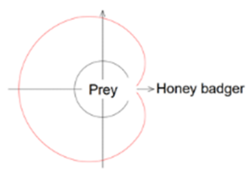
2.1. Introduction to the Honey Badger Algorithm (HBA)

This section gives a brief introduction to the HBA. For detailed analysis, please refer to [13]. The honey badger is a large weasel, mostly living in tropical rain forests and open grassland areas in Africa. When HBA solves the parameter optimization problem, it can be divided into “digging” and “honey”. The following describes the model of the HBA, where $r_i$ represents a random number from 0–1:

The total X of candidate solutions in HBA is expressed as:

$$X=\left[\begin{array}{llll}{x}_{11}& x_{12}& \cdot \cdot \cdot & x_{1D}\\ x_{21}& x_{22}& \cdot \cdot \cdot & x_{2D}\\ & \cdot \cdot \cdot \cdot & \cdot \cdot \cdot \cdot & \cdot \cdot \cdot \cdot \\ x_{n1}& x_{n2}& \cdot \cdot \cdot & x_{nD}\end{array}\right]$$

(1)

The mathematical expression for the location of the ith honey badger is: $x_i=\left[{x_i}^1,{x_i}^2,\dots ,{x_i}^D\right]$.

Step 1: Initialization. The number and location of honey badgers are initialized by Equation (2).

$$x_i={lb}_i+r_1\times ({ub}_i-{lb}_i)$$

(2)

where $x_i$ is a positional parameter, which is a candidate solution, and ${ub}_i$ and ${lb}_i$ are the range of the target parameter values.

Step 2: Define intensity ($I$). Predation intensity is related to the concentration intensity of prey and the distance between prey and honey badger. I_i is defined by Equation (3) and represents the scent intensity of prey.

$$\begin{array}{l}{I}_i=r_2\times \frac{S}{4\pi {d_i}^2}\\ S={(x_i-x_i+1)}^2\\ d_i=x_{prey}-x_i\end{array}$$

(3)

where $S$ represents concentrated intensity (Figure 1 shows the location of the prey), and $d_i$ represents the distance between prey and the ith generation badger.

Step 3: Density factor ($\alpha$). $\alpha$ controls the randomness of changes over time to ensure a reasonable transition from exploration to development. The updated formula is shown in Equation (4).

$$\alpha =A\times \exp (-\frac{n}{n_{\max }})$$

(4)

where $n$ represents the current iteration number, $A$ represents a constant (default $A$ = 2), and $n_{\max }$ represents the maximum iteration number.

Step 4: To avoid local optimization, HBA introduces parameters to change the search direction and improve the search ability.

Step 5: Update the population location.

Digging phase: as shown in Figure 2, the movement of the honey badger at this stage is simulated as a heart (the circle is the location of the honey badger, and the heart line is the odor intensity range). The movement track of the honey badger is simulated by Equation (5):

$$\begin{array}{lll}{x}_{new}& =& x_{prey}+Q\times \gamma \times I\times x_{prey}\\ & +& Q\times r_3\times \alpha \times d_i\times \left|\cos (2\pi r_4)-\cos (2\pi r_4)\ast \cos (2\pi r_5)\right|\end{array}$$

(5)

where $x_{prey}$ represents the global optimal location, $\gamma$ represents the power of honey badger to obtain food (default $\gamma =6$), and parameter $Q$ controls the search direction, which is determined by Equation (6):

$$Q=\left\{\begin{array}{ll}1& r_6\le 0.5\\ -1& \mathrm{else}\end{array}\right.$$

(6)

Honey phase: The process by which the guide bird leads the honey badger to the hive is determined by Equation (7):

$$x_{new}=x_{prey}+Q\times r_7\times \alpha \times d_i$$

(7)

where $x_{new}$ represents the new location of honey badger, and $x_{prey}$ is the location of prey.

2.2. Variational Modal Decomposition (VMD)

This section gives a brief introduction to VMD. VMD has been widely used in the field of fault diagnosis since it was proposed. VMD decomposes non-stationary signals into several IMFs in a non-recursive form [29], and the mathematical expression of component $u_k$ is:

$$u_k=a_k(t)\cos ({\phi }_k(t))$$

(8)

where $a$ is the amplitude, and $\phi$ is the phase.

The Hilbert transform is applied to $u_k$, and the bandwidth of each mode can be obtained from Equation (9):

$$(\delta (t)+\frac{j}{\pi t})\times u_k(t)$$

(9)

where $\delta (t)$ is the Dirichlet function, and $\ast$ is the convolution operator. Equation (8) is multiplied by the exponential term, and the spectrum is transformed into the central frequency band, as shown in Equation (10).

$$\left[(\delta (t)+\frac{j}{\pi t})\times u_k(t)\right]e^{j\omega kt}$$

(10)

where $\left\{{\omega }_k\right\}=\left\{{\omega }_1,{\omega }_2\cdot \cdot \cdot {\omega }_K\right\}$ is the center frequency, $\left\{u_k\right\}=\left\{u_1,u_2\dots u_K\right\}$ is the K modes after decomposition, and the bandwidth of the component is estimated by the square of the modulated signal $L^2$ norm, with the sum of the minimum bandwidth as the constraint condition, as shown in Equation (11):

$$\underset{\left\{u_k\right\},\left\{{\omega }_k\right\}}{\min }\left\{{{\displaystyle \sum _k‖\partial t\left[\left(\delta (t)+\frac{j}{\pi t}\right)\times u_k(t)\right]e^{-j\omega kt}‖}}_2^2\right\}$$

(11)

The sum of all components $u_k$ is the original signal $f$, $f={\displaystyle \sum _k{u}_k}$.

$$\begin{array}{l}L(\{u_k\},\{{\omega }_k\},\lambda )=\alpha {{\displaystyle \sum _k‖{\partial }_t\left[\left(\delta (t)+\frac{j}{\pi t}\right)\times u_k(t)\right]e^{-j\omega kt}‖}}_2^2\\ +{‖f(t)-{\displaystyle \sum _k{u}_k(t)}‖}_2^2+〈\lambda (t),f(t)-{\displaystyle \sum _k{u}_k(t)}〉\end{array}$$

(12)

ADMM [5] is used when selecting the optimal solution, as shown below:

$${\widehat{u}}_k^{n+1}(\omega )=\frac{f(\omega )-{\displaystyle \sum {}_{i=1}^{K-1}}{\widehat{u}}_i^{n+1}(\omega )+\frac{\widehat{\lambda }(\omega )}{2}}{1+2\alpha {(\omega -{\omega }_k)}^2}$$

(13)

$${\omega }_k^{n+1}=\frac{{\displaystyle {\int }_0^{\infty }\omega {\left|{\widehat{u}}_k^{n+1}(\omega )\right|}^{2}d\omega }}{{\displaystyle {\int }_0^{\infty }{\left|{\widehat{u}}_k^{n+1}(\omega )\right|}^{2}d\omega }}$$

(14)

$${\widehat{\lambda }}^{n+1}(\omega )=\widehat{\lambda }(\omega )+\tau \left(\widehat{f}-{\displaystyle \sum _{k=1}^K{\widehat{u}}_k^{n+1}(\omega )}\right)$$

(15)

where $n$ represents the number of iterations, ^ represents the Fourier transform, $\tau$ represents the Lagrange multiplier sub-step, and the center frequency and bandwidth of each component are iterated and updated until the condition of Equation (16) is met:

$${\displaystyle \sum _{k=1}^K\left({‖{\widehat{u}}_k^{n+1}(\omega )-{\widehat{u}}_k^n(\omega )‖}_2^2/{‖{\widehat{u}}_k^n(\omega )‖}_2^2\right)}<\epsilon$$

(16)

where $\epsilon$ stands for tolerance.

Previous studies have proved that VMD decomposition layers $K$ and penalty factor $\alpha$ are the key parameters affecting VMD decomposition performance. In this paper, the CHBA is used to optimize VMD and select the optimal parameters.

2.3. Extreme Learning Machine (ELM)

This section gives a brief introduction to ELM. The mathematical model of ELM is as follows: Suppose that N training samples are expressed as:

$$N=\{(x_i,t_i)\left|x_i\in R^n,t_i\right.\in R^m,i=1,2,\cdot \cdot \cdot ,N\}$$

(17)

The neural network mathematical model with m input layer nodes, n output layer nodes and L hidden layer nodes is as follows:

$${\displaystyle \sum _{i=1}^L{\beta }_i}p(a_i{x}_j+b_i)=t_j j=1,2,\cdot \cdot \cdot ,N$$

(18)

where $p(x)$ is the activation function, $a_i={[a_{i1},a_{i2},\dots ,a_{im}]}^T$ is the input weight matrix, ${\beta }_i={[{\beta }_{i1},{\beta }_{i2},\dots ,{\beta }_{in}]}^T$ is the output weight matrix of the hidden layer, $b_i$ is the threshold of the hidden layer, and $t_i={[t_{i1},t_{i2},\dots ,t_{in}]}^T$ is the network output matrix.

Equation (18) is expressed in the following matrix form:

$$K\beta =T$$

(19)

where $K={\left[\begin{array}{ccc}p(a_1{x}_1+b_1)& \cdots & p(a_L{x}_1+b_L)\\ ⋮& & ⋮\\ p(a_1{x}_N+b_1)& \cdots & p(a_L{x}_N+b_L)\end{array}\right]}_{N\times L}$ represents the output of the hidden layer, $\beta ={[{\beta }_1,{\beta }_2,\cdots ,{\beta }_L]}^T$ represents the output weight, and $T={[T_1,T_2,\cdots ,T_N]}^T$ represents the target output.

When $p(x)$ is infinitely differentiable, ELM randomly selects the input weight and the threshold of the hidden layer, and the matrix $K$ remains unchanged during training, so the training process of ELM is to find the least square solution $\widehat{\beta }$.

$$\widehat{\beta }=K^{+}T$$

(20)

where $K^{+}$ represents the generalized inverse of the matrix $K$.

3. Proposed Method

3.1. Chaotic Mapping-Improved Honey Badger Algorithm (CHBA)

Chaotic behavior is a nonlinear random phenomenon, and has been widely used in algorithm optimization due to its excellent performance. Introducing chaotic mapping into the algorithm can successfully solve the drawbacks of setting into local optimum or slow convergence. Common chaotic mapping includes the sine map, Circle map, Logistic map, Iterative Map, etc.; examples include the hybrid strategy improved sparrow search algorithm [30], the nonlinear chaotic Harris–Eagle algorithm [31], the chaotic map optimized gray wolf algorithm [32], and the hybrid strategy improved whale optimization algorithm [33]. Through the above inspiration and analysis, we propose a new chaotic honey badger algorithm (CHBA), in which chaotic values are used instead of random values in the updating stage of the population position. Therefore, Equations (5) and (7) are rewritten as follows:

$$\begin{array}{lll}{x}_{new}& =& x_{prey}+Q\times \gamma \times I\times x_{prey}\\ & +& Q\times {cm}_1\times \alpha \times d_i\times \left|\cos (2\pi {cm}_2)\times \left[1-\cos (2\pi {cm}_3)\right]\right|\end{array}$$

(21)

$$x_{\mathrm{new}}=x_{prey}+Q\times {cm}_4\times \alpha \times d_i$$

(22)

where ${cm}_i$ is the sinusoidal chaos number generated in each iteration.

3.2. CHBA Optimizes VMD and ELM

CHBA-VMD Model

The Gini index (GI) is an indicator of the income gap of residents in a country or region, and has been used in fault diagnosis in recent years. In 2017, Miao, et al. [34] improved kurtogram and ProTrugram by substituting GI for the kurtogram index of the signal, and confirmed the robustness of GI to impulse noise for the first time. Albezzawy, et al. [35] replaced kurtogram with GI to achieve optimal modal extraction of wavelet decomposition. In 2021, Miao, et al. [36] proposed the Gini index of the square envelope (GISE). This paper verifies that GISE is a suitable time domain index affecting GI performance In this paper, the maximum value of GISE is taken as the criterion to establish the CHBA-VMD model, and the optimal VMD parameters for decomposition of different fault signals are adaptively selected. The GISE value of the signal can be calculated as follows:

$$GISE=1-2{\displaystyle \sum _{n=1}^N\left(SE(n)/{‖SE‖}_1\right)}\left(N-n+0.5/N\right)$$

(23)

where, $SE={\left|s\right|}^2$ and its order $S{E}_{order}=[S{E}_{(1)}\cdots S{E}_{(i)}\cdots S{E}_{(N)}]$, $S{E}_{(1)}\le \cdots \le S{E}_{(i)}\cdots S{E}_{(N)}$, and $S{E}_{(n)}$ represents the nth element in vector $SE$.

To make up for the deficiency of ELM and improve the classification accuracy, the CHBA-ELM model was established to adaptively select the optimal initial weight and threshold value of ELM. The fitness function is shown in Equation (24):

$$fitness=argmin(Erro{r}_1+Erro{r}_2)$$

(24)

where $argmin$ represents the minimum value, $Erro{r}_1$ represents the error rate of training set, and $Erro{r}_2$ represents the error rate of testing set.

3.3. Feature Extraction

Systematic sampling is a common method in statistics to study the characteristics and rules of numbers. It has the advantages of simplicity, convenience and good sample representativeness. Its mathematical definition is as follows: N samples are selected from N samples, with $K=[N/n]$ as the sampling interval ($[\cdot ]$ represents the integer function), and a number I is randomly selected from 1~K, so the N samples are $i,i+k\cdots i+(n-1)k$.

In this paper, the “Systematic Sampling Method (SSM)” is used to group the signals decomposed by VMD. Assuming that a group of signals is $Y=[y_1,y_2,y_3,\cdots ,y_N]$, n numbers are extracted from them as a group, and the sampling interval is $K=[N/n]$. The data is divided into k groups:

$$A=\left[\begin{array}{c}{y}_1(1),y_{1+K}(2)\cdots y_{1+(n-1)K}(n)\\ y_2(1),y_{2+K}(2)\cdots y_{2+(n-1)K}(n)\\ \cdots \\ y_K(1),y_{K+K}(2)\cdots y_{K+(n-1)K}(n)\end{array}\right]$$

(25)

The energy component feature vector $E$($E={[E_1,E_2,E_3,\cdots ,E_K]}^T$) of each group of signals in $A$ is calculated, and the energy calculation equation is as follows:

$$E_i={\displaystyle \sum _{n=1}^n{y}_i{(n)}^2}$$

(26)

3.4. Fault Diagnosis Model

To sum up, combined with the excellent performance of CHBA, VMD and ELM, this paper propose a composite fault diagnosis model of CHBA-VMD-CHBA-ELM. The basic process is shown in Figure 3, and the main process has the following four steps:

Step 1: The chaotic honey badger algorithm optimizes variational modal decompositions, selects the optimal parameters of signals of different fault types [$k$, $\alpha$], and decomposes the signals into several IMF components by using the selected optimal parameters.

Step 2: Using the Gini index of square envelope as the criterion, the GISE value of the IMF component is calculated and the four largest components are selected.

Step 3: The “SSM” is used to group the signals of each component and calculate the energy composition of high-dimensional fault feature vectors.

Step 4: The chaotic honey badger algorithm optimizes the extreme learning machine, selects the optimal parameters of ELM, and inputs the high-dimensional fault feature vector into the CHBA-ELM model to classify and recognize different types of fault signals.

4. Analysis of the Influence of Chaotic Mapping on the Performance of HBA

4.1. Low-Dimensional Single-Objective Test Function

To test the performance of CHBA, the whale optimization algorithm (WOA), honey badger algorithm (HBA), moth-flame optimization algorithm (MFO), gray wolf optimization algorithm (GWO) and chaos honey badger algorithm (CHBA) were selected for comparative analysis. The parameter settings of the algorithm are shown in

Table 1. Algorithm parameter settings.

Name of the Algorithm	Name of the Parameter
MFO	Convergence factor a: [−2 −1]
WOA	Convergence factor a: [2 0]
GWO	Convergence factor a: [2 0]
HBA	The ability to get food $\gamma =6$, constant $A=2$
CHBA	The ability to get food $\gamma =6$, constant $A=2$

. The maximum number of iterations was set as 600, and the population number was set as 100.

Table 2. Seven high-dimensional single objective functions (Dim = 30).

Function	Range	${\mathit{F}}_{\mathit{m}\mathit{i}\mathit{n}}$
$f_1(x)={\displaystyle \sum _{i=1}^n{x}_i{}^2}$	[−100,100]	0
$f_2(x)={\displaystyle \sum _{i=1}^n\left|x_i\right|}+{\displaystyle \prod _{i=1}^n\left|x_i\right|}$	[−10,10]	0
$f_3(x)={{\displaystyle \sum _{i=1}^n\left({\displaystyle \sum _{j=1}^i{x}_j}\right)}}^2$	[−100,100]	0
$f_4(x)=max\left\{\left|x_i\right|,1\le i\le n\right\}$	[−100,100]	0
$f_5(x)={\displaystyle \sum _{i=1}^{n-1}\left[100{(x_{i+1}-x_i{}^{{}_2})}^2+{(x_i-1)}^2\right]}$	[−30,30]	0
$f_6(x)={{\displaystyle \sum _{i=1}^n\left(\left[x_i+0.5\right]\right)}}^2$	[−100,100]	0
$f_7(x)={\displaystyle \sum _{i=1}^{n}i{x}_i{}^4}+random[0,1)$	[−1.28,1.28]	0

shows seven low-dimensional single-objective test functions. Such functions have only one global optimal solution, which can test the convergence and local development performance of the algorithm. Each test function is tested for 30 times independently, and the average value and standard deviation are recorded to test the convergence accuracy and stability of the algorithm. The results are shown in Appendix A.

4.1.1. Analysis of Convergence Accuracy and Stability

It can be seen from Appendix A that CHBA can calculate the minimum mean value and variance of functions $f_1(x)~f_4(x)$ and $f_7(x)$, and obtain the optimal solution of functions $f_1(x)$ and $f_3(x)$, proving that its convergence accuracy and stability are better than the other five algorithms. For function $f_5(x)$, HHO has the highest convergence accuracy and stability. For function $f_6(x)$, HBA has the best convergence accuracy and stability.

4.1.2. Analysis of Convergence Speed

The curves of the seven high-dimensional single-objective functions are shown in Figure 4. For $f_1(x)~f_4(x)$ and $f_7(x)$, the CHBA algorithm has the fastest convergence speed. For functions $f_5(x)$ and $f_6(x)$, although the CHBA algorithm has poor convergence accuracy and stability, its convergence speed is the fastest. The results show that the overall performance of CHBA is better than other algorithms in the high-dimensional single-objective test function.

4.2. High-Dimensional Multi-Objective Test Function

Table 3. Five high-dimensional multi-objective test functions (Dim = 30).

Function	Range	$\mathit{F}\mathit{m}\mathit{i}\mathit{n}$
$f_8(x)={\displaystyle \sum _{i=1}^n-x_i\sin (\sqrt{\left|x_i\right|})}$	[−500,500]	−418.9829n
$f_9(x)={\displaystyle \sum _{i=1}^n[x_i{}^2-10\cos (2\pi x_i)+10]}$	[−5.12,5.12]	0
$\begin{array}{l}{f}_{10}(x)=-20\exp (-0.2\sqrt{\frac{1}{n}{\displaystyle \sum _{i=1}^n{x}_i{}^2}})\\ -\exp (\frac{1}{n}{\displaystyle \sum _{i=1}^n\cos (2\pi x_i)})+20+e\end{array}$	[−32,32]	0
$f_{11}(x)=\frac{1}{4000}{\displaystyle \sum _{i=1}^n{x}_i{}^2-{\displaystyle \prod _{i=1}^n\cos (\frac{x_i}{\sqrt{i}})}}+1$	[−600,600]	0
$\begin{array}{l}{f}_{12}(x)=\frac{\pi }{n}\left\{10\sin (\pi y_1)+{\displaystyle \sum _{i=1}^{n-1}{(y_i-1)}^2[1+10{\sin }^2(\pi y_{i+1})]+{(y_n-1)}^2}\right\}\\ +{\displaystyle \sum _{i=1}^{n}u(x_i,10,100,4),y_i=1+\frac{x_i+1}{4}}\\ u(x_i,a,k,m)=\left\{\begin{array}{ll}k{(x_i-a)}^m& x_i>a\\ 0& -1<x_i<a\\ k{(-x_i-a)}^m& x_i<-a\end{array}\right.\end{array}$	[−50,50]	0

shows five kinds of high-dimensional multi-objective test functions, with one global optimal solution and several local optimal solutions, which are used to test the local and global search ability of the algorithm. Thirty independent tests were conducted for each test function, and the mean value and standard deviation were calculated to verify the convergence accuracy and stability of the algorithm. The results are shown in Appendix A.

4.2.1. Analysis of Convergence Accuracy and Stability

It can be seen from Appendix A, for function $f_8(x)$, HHO has the best convergence accuracy and stability, and can accurately find the optimal solution, while the CHBA algorithm cannot find the optimal solution. For function $f_9(x)$, except the MFO algorithm, other algorithms have the same convergence accuracy and stability, and can find the optimal solution accurately. For function $f_{10}(x)$ and $f_{11}(x)$, HBA, HHO and CHBA, the performance is the same and the effect is excellent. For function $f_{12}(x)$, the HBA algorithm has the best convergence accuracy and stability, while CHBA cannot find the optimal solution.

4.2.2. Analysis of Convergence Speed

The curves of the five high-dimensional multi-objective test functions are shown in Figure 5. For functions $f_8(x)$ and $f_{12}(x)$, CHBA cannot find the optimal solution, but the convergence speed is the fastest. For the other three functions, CHBA can find the optimal solution and has the fastest convergence speed. The overall performance of the high-dimensional multi-objective test function is better than other algorithms.

4.3. Low-Dimensional Test Function

To more comprehensively test the convergence speed, stability, and accuracy of HBA, the following ten fixed-dimensional functions are selected for testing, as shown in

Table 4. Fixed-dimension test functions.

Function	Dim	Range	$\mathit{F}\mathit{m}\mathit{i}\mathit{n}$
$f_{13}(x)={\left(\frac{1}{500}+{\displaystyle \sum _{j=1}^{25}\frac{1}{j+{\displaystyle \sum _{i=1}^2{(x_i-a_i{}_j)}^6}}}\right)}^{-1}$	2	[−65,65]	1
$f_{14}(x)={{\displaystyle \sum _{i=1}^{11}\left[ai-\frac{x_1(b_i{}^2+b_i{x}_2)}{b_i{}^2+b_i{x}_3+x_4}\right]}}^2$	4	[−5,5]	0.003
$f_{15}(x)=4x_1{}^2-2.1x_1{}^4+\frac{1}{3}{x}_1{}^6+x_1{x}_2-4x_2{}^2+4x_2{}^4$	2	[−5,5]	−1.0316
$f_{16}(x)={\left(x_2-\frac{5.1}{4{\pi }^2}{x}_1{}^2+\frac{5}{\pi }{x}_1-6\right)}^2+10\left(1-\frac{1}{8\pi }\right)\cos x_1+10$	2	[−5,5]	0.398
$\begin{array}{l}{f}_{17}(x)=[1+{(x_1+x_2+1)}^2(19-{14x}_1+{{3x}_1}^2-{14x}_2+{6x}_1{x}_2+{{3x}_2}^2)]\\ \times [30+{({2x}_1-{3x}_2)}^2\times (18-{32x}_1+{12x_1}^2+{48x}_2-{36x}_1{x}_2+{27x_2}^2)]\end{array}$	2	[−5,5]	3
$f_{18}(x)=-{\displaystyle \sum _{i=1}^4{c}_i\exp \left(-{\displaystyle \sum _{j=1}^3{a}_{ij}{(x_j-p_i{}_j)}^2}\right)}$	3	[0,1]	−3.86
$f_{19}(x)=-{\displaystyle \sum _{i=1}^4{c}_i\exp \left(-{\displaystyle \sum _{j=1}^6{a}_{ij}{(x_j-p_i{}_j)}^2}\right)}$	6	[0,1]	−3.32
$f_{20}(x)=-{{\displaystyle \sum _{i=1}^5\left[(X-a_i){(X-a_i)}^T+c_i\right]}}^{-1}$	4	[0,10]	−10.1532
$f_{21}(x)=-{{\displaystyle \sum _{i=1}^7\left[(X-a_i){(X-a_i)}^T+c_i\right]}}^{-1}$	4	[0,10]	−10.4028
$f_{22}(x)=-{{\displaystyle \sum _{i=1}^{10}\left[(X-a_i){(X-a_i)}^T+c_i\right]}}^{-1}$	4	[0,10]	−10.5363

. The results are shown in Appendix A.

4.3.1. Analysis of Convergence Accuracy and Stability

As can be seen from Appendix A, for the 10 low-dimensional test functions, CHBA has good stability and convergence accuracy. For $f_{15}(x)$, all six algorithms can obtain the optimal solution, but WOA and GWO have poor stability. For $f_{16}(x)$, the CHBA algorithm has the best stability. For $f_{17}(x)$, the six algorithms have the same convergence accuracy and stability. For $f_{18}(x)$, MFO, HBA, HHO and CHBA, the results are the same. For $f_{19}(x)$, $f_{21}(x)$ and $f_{22}(x)$, the CHBA algorithm is superior to others in terms of convergence accuracy and stability. For $f_{18}(x)$, the HBA and CHBA algorithm have the same results.

4.3.2. Analysis of Convergence Speed

The curves of the ten low-dimensional functions are shown in Figure 6. In general, the convergence speed of the CHBA algorithm is slightly better than that of other algorithms. For the function $f_{21}(x)$, although WOA and HHO algorithms converge faster than the CHBA algorithm, the CHBA algorithm has a higher convergence accuracy. Therefore, it indicates that the CHBA has the optimal performance in low-dimensional test functions.

After this analysis, it was shown that the proposed HBA based on chaos mapping had significantly improved convergence speed, stability and convergence accuracy compared with HBA, and could better solve practical engineering problems.

5. Experimental Study

5.1. Parameter Selection of VMD

To verify the feasibility of the method in this paper, the bearing fault data of Xi’an Jiaotong University in its full life cycle were selected for verification [37]. Six types of data were selected: normal, outer race fault, inner race fault, cage fault, inner race and outer race fault, and multi position fault of inner race, outer race, cage and rolling elements. The sampling frequency fs = 25,600 Hz, and the sampling number N = 10000. Different data were decomposed by CHBA-VMD, and the VMD parameter was set to a time-step of dual ascent $\tau =0$, tolerance $\epsilon =1\times {10}^{-9}$, and initial $\omega =0$, the settings of these three parameters are the same as in the original paper [5]. The range of $K$ and $\alpha$ was set to $[2,12]$ and $[100,2500]$, the range settings of these two parameters are based on previous research and experience. The optimal parameter values of VMD optimization by CHBA are shown in

Table 5. Optimal parameters of CHBA-VMD.

Fault Type	K	$\mathit{\alpha }$
Outer race	11	841
Normal	8	2117
Inner race	10	1474
The inner and outer race	8	328
Cage	6	280
Inner race, outer race, rolling elements and cage	9	265

. The number of the honey badger population was set to 10, and the maximum iteration was set to 20. The convergence curve of the maximum GISE value chosen by the CHBA to optimize the VMD is shown in Figure 7 (the data shown in the graph have been normalized).

5.2. Construction of Fault Feature Vector

The GISE of each IMF component after decomposition was calculated, as shown in Figure 8. The first four components with the largest GISE value were selected, as shown in Figure 9, which is the time domain diagram of each component, and each component was divided into 100 groups (see Section 3.3 for the method), that is, each group of data includes 100 samples, each type of fault consists of 100 × 4, and the labels of the six fault types are set as 1, 2, 3, 4, 5 and 6.

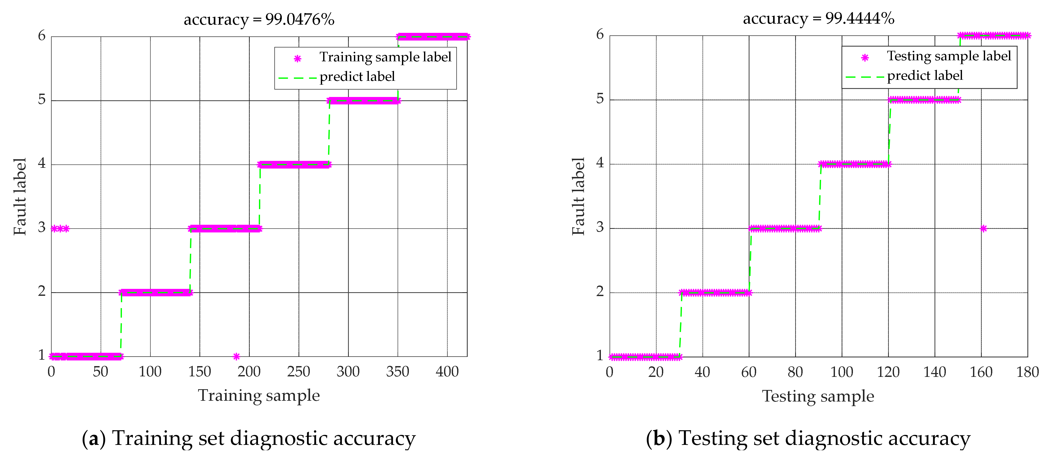
5.3. Classification Results

The training set and testing set samples are separated by 7:3. That is, a total of 420 samples were selected as the training set and 180 samples as the test set. The samples were input into BP, ELM, KELM, GA-ELM, GMO-ELM, HBA-ELM and CHBA-ELM models, and each classification model was trained ten times. The maximum, minimum and average accuracy of the training set and test set were recorded and compared, as shown in

Table 6. Comparison of classification results.

Algorithm	Accuracy of Training Set (%)			Accuracy of Testing Set (%)
	Min	Max	Mean	Min	Max	Mean
BP	59.52	89.76	71.24	63.89	95.56	77.77
ELM	97.00	98.67	98.33	76.33	80.33	78.17
GWO-ELM	98.57	98.81	98.76	95.00	97.78	96.39
HBA-ELM	95.24	98.81	97.26	96.11	99.44	97.50
CHBA-ELM	98.10	100.00	98.80	100.00	98.83	99.50

. The CHBA-ELM model had the highest classification accuracy and is superior to others; the classification results are shown in Figure 10.

To verify the influence of the “SSM” proposed in this paper on the classification results, the signals decomposed by CHBA-VMD were grouped in sequence to calculate the feature vector of energy composition and input into the CHBA-ELM classifier. The classification results are shown in Figure 11. Its classification accuracy is very poor; the accuracy rate has been lower than 80% in numerous trials. Thus, the advantages of the proposed “SSM” are verified.

6. Conclusions

This paper presents a new model for composite fault diagnosis of bearings. Aiming at addressing the deficiency of the honey badger algorithm, chaos mapping was introduced to improve it, and the superiority of CHBA was verified on 23 benchmark functions. Aiming at the problem that parameters in variational mode decomposition and extreme learning machine need to be set manually, a novel adaptive VMD is established based on VMD, and a novel adaptive ELM is established based on ELM. Compared with other models, the classification accuracy was up to 100%, which is superior to most existing methods and has better stability. In addition, this paper introduces the “SSM” in statistics to group the decomposed signals. Experimental verification shows that the “SSM” can better characterize data and improve classification accuracy. At the same time, a new index named GISE is introduced into fault diagnosis, which successfully solves the classification problem of rolling bearing composite faults. Although this method has a remarkable effect and obvious advantages, it may take too long to decompose complex signals using CHBA optimization VMD. Therefore, shortening the decomposition time and improving diagnostic efficiency is one of the research directions that need to be improved in the future.

References

1. Noshirvani, G.; Askari, J.; Fekih, A. A robust fault detection and isolation filter for the pitch system of a variable speed wind turbine. Int. Trans. Electr. Energy Syst. 2018, 28, e2625. [Google Scholar] [CrossRef]
2. Huang, N.; Shen, Z.; Long, S.; Wu, M.C.; Shih, H.H.; Zheng, Q.; Yen, N.; Tung, C.C.; Liu, H.H. The empirical mode decomposition and the Hilbert spectrum for nonlinear and non-stationary time series analysis. Proc. R. Soc. Lond. Ser. A 1998, 454, 903–995. [Google Scholar] [CrossRef]
3. Amrinder, S.M.; Gurpreet, S.; Jagpreet, S.; Kankar, P.K.; Sukhjeet, S. A novel method to classify bearing faults by integrating standard deviation to refined composite multi-scale fuzzy entropy. Measurement 2020, 154, 107441. [Google Scholar]
4. Zheng, J.; Su, M.; Ying, W.; Tong, J.; Pan, Z. Improved uniform phase empirical mode decomposition and its application in machinery fault diagnosis. Measurement 2021, 179, 109425. [Google Scholar] [CrossRef]
5. Dragomiretskiy, K.; Zosso, D. Variational Mode Decomposition. IEEE Trans. Signal Process. 2014, 62, 531–544. [Google Scholar] [CrossRef]
6. Ye, M.; Yan, X.; Jia, M. Rolling Bearing Fault Diagnosis Based on VMD-MPE and PSO-SVM. Entropy 2021, 23, 762. [Google Scholar] [CrossRef] [PubMed]
7. Fu, W.; Shao, K.; Tan, J.; Wang, K. Fault Diagnosis for Rolling Bearings Based on Composite Multiscale Fine-Sorted Dispersion Entropy and SVM With Hybrid Mutation SCA-HHO Algorithm Optimization. IEEE Access 2020, 8, 13086–13104. [Google Scholar] [CrossRef]
8. Zhang, F.; Sun, W.; Wang, H.; Xu, T. Fault Diagnosis of a Wind Turbine Gearbox Based on Improved Variational Mode Algorithm and Information Entropy. Entropy 2021, 23, 794. [Google Scholar] [CrossRef]
9. Li, Y.; Peng, Z. Fault Diagnosis of Rolling Bearing Based on Parameter Adaptive VMD. Noise Vib. Control. 2021, 41, 139–146. [Google Scholar]
10. Liang, T.; Lu, H.; Sun, H. Application of Parameter Optimized Variational Mode Decomposition Method in Fault Feature Extraction of Rolling Bearing. Entropy 2021, 23, 520. [Google Scholar] [CrossRef]
11. Zhi, L.; Hu, F.; Zhao, C.; Wang, J. Modal parameter estimation of civil structures based on improved variational mode decomposition. Struct. Eng. Mech. 2021, 79, 683–697. [Google Scholar]
12. Mganb, C.; Tmh, A.; Om, A. An adaptive variational mode decomposition based on sailfish optimization algorithm and Gini index for fault identification in rolling bearings. Measurement 2020, 173, 108514. [Google Scholar]
13. Hashim, F.A.; Houssein, E.H.; Hussain, K.; Mabrouk, M.S.; Al-Atabany, W. Honey Badger Algorithm: New Metaheuristic Algorithm for Solving Optimization Problems. Math. Comput. Simul. 2021, 192, 84–110. [Google Scholar] [CrossRef]
14. Wang, C. A sample entropy inspired affinity propagation method for bearing fault signal classification. Digit. Signal Process. 2020, 102, 102740. [Google Scholar] [CrossRef]
15. Deng, W.; Yao, R.; Sun, M.; Zhao, H.; Luo, Y.; Dong, C. Study on a novel fault diagnosis method based on integrating EMD, fuzzy entropy, improved PSO and SVM. J. Vibroeng. 2017, 19, 2562–2577. [Google Scholar]
16. Hou, J.; Wu, Y.; Gong, H.; Ahmad, A.S.; Liu, L. A novel intelligent method for bearing fault diagnosis based on EEMD permutation entropy and GG clustering. Appl. Sci. 2020, 10, 386. [Google Scholar] [CrossRef] [Green Version]
17. Ding, F.; Xia, Y.; Tian, J.; Zhang, X. An AVMD Method Based on Energy Ratio and Deep Belief Network for Fault Identification of Automation Transmission Device. IEEE Access 2021, 9, 150088–150097. [Google Scholar] [CrossRef]
18. Zhou, R.; Wang, X.; Wan, J.; Xiong, N. EDM-Fuzzy: An Euclidean Distance Based Multiscale Fuzzy Entropy Technology for Diagnosing Faults of Industrial Systems. IEEE Trans. Ind. Inform. 2021, 17, 4046–4054. [Google Scholar] [CrossRef]
19. Udmale, S.S.; Singh, S.K. Bearing Fault Classification Using Wavelet Energy and Autoencoder; Springer Nature: Cham, Switzerland, 2020; Volume 25, pp. 227–238. [Google Scholar]
20. Shi, P.; Guo, X.; Han, D.; Fu, R. A sparse auto-encoder method based on compressed sensing and wavelet packet energy entropy for rolling bearing intelligent fault diagnosis. J. Mech. Sci. Technol. 2020, 34, 1445–1458. [Google Scholar] [CrossRef]
21. Gao, T.; Yang, J.; Jiang, S. A Novel Incipient Fault Diagnosis Method for Analog Circuits Based on GMKL-SVM and Wavelet Fusion Features. IEEE Trans. Instrum. Meas. 2020, 70, 3502315. [Google Scholar] [CrossRef]
22. Song, S.; Qiu, D.; Qin, S. Research on the Fault Diagnosis Method of Mine Fan Based on Sound Signal Analysis. Adv. Civ. Eng. 2021, 9650644. [Google Scholar] [CrossRef]
23. Huang, G.B.; Chen, Y.Q.; Babri, H.A. Classification ability of single hidden layer feedforward neural networks. IEEE Trans. Neural Netw. 2000, 11, 799–801. [Google Scholar] [CrossRef] [PubMed] [Green Version]
24. Xiao, J.; Zhou, J.; Li, C.; Xiao, H.; Zhang, W.; Zhu, W. Multi-fault classification based on the two-stage evolutionary extreme learning machine and improved artificial bee colony algorithm. Proc. Inst. Mech. Eng. Part C J. Mech. Eng. Sci. 2013, 228, 1797–1807. [Google Scholar] [CrossRef]
25. Qin, Y.L.; Liu, J.G.; Wang, Y.Z. Rolling bearing fault diagnosis method based on extreme learning machine. Mod. Mach. Tool Autom. Manuf. Technol. 2016, 5, 103–106. [Google Scholar]
26. Wang, T.T.; Wang, Y.; Ji, Z.C. Rolling bearing fault diagnosis based on improved extreme learning machine. J. Syst. Simul. 2018, 30, 4413–4420. [Google Scholar]
27. Cheng, H.; Wu, T.; Gu, R.; Jin, Z.; Ma, R.; Qu, H. Rolling bearing fault diagnosis based on composite multiscale permutation entropy and reverse cognitive fruit fly optimization algorithm–Extreme learning machine-ScienceDirect. Measurement 2020, 173, 108636. [Google Scholar]
28. Wang, H.; Jing, W.; Li, Y.; Yang, H. Fault Diagnosis of Fuel System Based on Improved Extreme Learning Machine. Neural Process. Lett. 2020, 53, 2553–2565. [Google Scholar] [CrossRef]
29. Liu, C.; Tan, J.; Huang, Z. Fault Diagnosis of Rolling Element Bearings Based on Adaptive Mode Extraction. Machines 2022, 10, 260. [Google Scholar] [CrossRef]
30. Zhang, C.; Ding, S. A stochastic configuration network based on chaotic sparrow search algorithm. Knowl.-Based Syst. 2021, 220, 106924. [Google Scholar] [CrossRef]
31. Dehkordi, A.A.; Sadiq, A.S.; Mirjalili, S.; Ghafoor, K.Z. Nonlinear-based Chaotic Harris Hawks Optimizer: Algorithm and Internet of Vehicles application. Appl. Soft Comput. 2021, 109, 107574. [Google Scholar] [CrossRef]
32. Xu, Z.; Yang, H.; Li, J.; Zhang, X.; Lu, B. Comparative Study on Single and Multiple Chaotic Maps Incorporated Grey Wolf Optimization Algorithms. IEEE Access 2021, 9, 77416–77437. [Google Scholar] [CrossRef]
33. Xu, H.; Zhang, D.; Wang, Y.; Song, T.; Fan, Y. Hybrid strategy improved whale optimization algorithm. Comput. Eng. Des. 2020, 41, 3397–3404. [Google Scholar]
34. Miao, Y.; Wang, J.; Zhang, B.; Li, H. Improvement of kurtosis-guided-grams via Gini index for bearing fault feature identification. Meas. Sci. Technol. 2017, 28, 12. [Google Scholar] [CrossRef]
35. Albezzawy, M.N.; Nassef, M.G.; Elsayed, E.S.; Elkhatib, A. Early Rolling Bearing Fault Detection Using A Gini Index Guided Adaptive Morlet Wavelet Filter. In Proceedings of the 10th International Conference on Mechanical and Aerospace Engineering (ICMAE), Brussels, Belgium, 22–25 July 2019; pp. 314–322. [Google Scholar]
36. Miao, Y.; Wang, J.; Zhang, B.; Li, H. Practical framework of Gini index in the application of machinery fault feature extraction. Mech. Syst. Signal Processing 2022, 165, 108333. [Google Scholar] [CrossRef]
37. Wang, B.; Lei, Y.G.; Li, N.P.; Li, N. A hybrid prognostics approach for estimating remaining useful life of rolling element bearings. IEEE Trans. Reliab. 2018, 69, 401–412. [Google Scholar] [CrossRef]
Figure 1. Prey location map (Inverse square law).
Machines 10 00469 g001
Figure 2. Schematic diagram of honey badger movement in excavation stage.
Machines 10 00469 g002
Figure 3. Flowchart of fault diagnosis.
Machines 10 00469 g003
Figure 4. Convergence curve of high-dimensional single objective function.
Machines 10 00469 g004aMachines 10 00469 g004b
Figure 5. Convergence curve of high-dimensional single objective function.
Machines 10 00469 g005
Figure 6. Convergence curve of low-dimensional test function.
Machines 10 00469 g006aMachines 10 00469 g006b
Figure 7. The convergence curve of the maximum GISE.
Machines 10 00469 g007
Figure 8. Comparison of GISE values of various components.
Machines 10 00469 g008aMachines 10 00469 g008b
Figure 9. Time domain diagram of fault signal.
Machines 10 00469 g009aMachines 10 00469 g009b
Figure 10. Classification results of CHBA-VMD-CHBA-ELM.
Machines 10 00469 g010
Figure 11. Classification results of “SSM”.
Machines 10 00469 g011