Article

A Fault Diagnosis Method of Rolling Bearings Based on Parameter Optimization and Adaptive Generalized S-Transform

School of Electrical and Electronic Engineering, Shanghai Institute of Technology, Shanghai 201418, China
*
Author to whom correspondence should be addressed.
Machines 2022, 10(3), 207; https://doi.org/10.3390/machines10030207
Submission received: 30 January 2022 / Revised: 9 March 2022 / Accepted: 10 March 2022 / Published: 14 March 2022
(This article belongs to the Special Issue Advances in Bearing Modeling, Fault Diagnosis, RUL Prediction)

Abstract

:
As for the fault diagnosis of rolling bearings under strong background noises, whether the fault feature extraction is comprehensive and accurate is critical, especially for the data-driven fault diagnosis methods. To improve the comprehensiveness and accuracy of the fault feature extraction, a fault diagnosis method of rolling bearings is proposed based on parameter optimization and Adaptive Generalized S-Transform (AGST). The AGST is used to solve the problem of incomplete feature extraction of bearing faults. The Particle Swarm Brain Storm Optimization algorithm based on the Discussion Mechanism (PSDMBSO) is used for the parameter optimization of VMD, which can better separate the complete fault components. The effectiveness of the fault diagnosis method proposed in this paper is verified by comparison with other methods.

1. Introduction

The rolling bearing occupies a vital position in most rotary machines. If the rolling bearing faults occur, it might lead to the parts of rotary machines being extremely easily damaged and even equipment collapse. Therefore, it is extremely important to diagnose the fault category of the bearing in time and accurately. The current mainstream rolling bearing fault diagnosis models are divided into three types: the diagnosis methods based on expert systems [1,2], the diagnosis methods based on analytical models [3,4], and the diagnosis methods based on data-driven models [5,6]. The diagnosis accuracy of the diagnosis method based on the expert system depends on the richness of expert experience and the level of knowledge, and the diagnosis method based on the analytical model relies on the accurate mathematical model of the diagnosed object. Therefore, these deficiencies limit its application in some actual environments. Compared with the above two methods, the data-driven diagnosis method is more practical for it diagnoses faults based on the historical data of the system and does not rely on accurate analytical models and rich expert knowledge.
As for the fault diagnosis method based on data-driven models, the capability of feature extraction has significant effects on the accuracy of fault diagnosis. In the early days, fault features were manually extracted from the vibration acceleration signals of rolling bearings [7]. At present, the vibration signal in different forms is used to improve a more accurate and sufficient feature extraction [8,9]. However, the effect of the signal processing method is often limited by the quality of the parameters, and so the optimization of the parameters becomes very important. Li proposed a bearing fault diagnosis method based on Particle Swarm Optimization Maximum Correlated Kurtosis Deconvolution (MCKD). The three parameters of MCKD were optimized by Particle Swarm Optimization to achieve effective enhancement of fault characteristics [10]. Tong proposed a rolling bearing fault diagnosis model based on the combination of VMD and Bayesian networks based on parameter optimization, and the parameters of VMD were optimized by variable-step Particle Swarm Optimization to improve the effectiveness of feature extraction [11]. Li proposed a VMD parameter optimization method based on the maximum envelope kurtosis and frequency band entropy and completed the identification of fault types through the envelope frequency spectrum [12]. Liu proposed a diagnosis model based on parameter optimization VMD and sample entropy. The genetic variation Particle Swarm Optimization algorithm was used for parameter optimization, which reduced the influence of parameters to a certain extent [13]. However, there are still existed the problem of manual selection in the selection of modal components. On this basis, Tang proposed the concept of envelope entropy by combining the sparse characteristics of vibration signals and used it as a fitness function to realize the adaptive optimization of modal component selection [14]. In addition, Liu constructed a band-pass filter based on the concept of frequency band entropy, and on this basis proposed a screening criterion for reconstruction components based on band entropy. The experimental results showed the effectiveness of the method [15].
However, with regards to the screening of VMD decomposition results, the key feature of different modal components between the fault state and the normal state needs to be captured more clearly. Based on these questions, contents related to neural networks are used to obtain sufficient fault features by increasing the comprehensiveness of feature extraction [16,17]. Since the one-dimensional convolutional neural network is prone to problems such as overfitting and missing features when dealing with vibration signals, it has become the mainstream trend to convert vibration signals into other forms of data. Xiao proposed a data processing method to convert the time domain signal into a two-dimensional grayscale image, and then applied it to the intelligent fault diagnosis of bearings [18]. By the method the depth of feature extraction is further improved but the adaptive ability of the model is reduced due to the fixed feature extraction scale. Shao proposed a fault diagnosis method for rotor-bearing systems under variable speed based on two-stage parameter transfer and infrared thermal imaging. The parameter transfer method enables the data (or parameters) acquired in the source domain to be applied in the target domain, which greatly enhances the adaptive ability of the system [19]. Luo proposed to use GST to convert the original signal into a two-dimensional time–frequency map, and adaptively change the time–frequency resolution through frequency changes to extract more sufficient time–frequency features [20]. However, due to the use of a relatively fixed scale factor, this method cannot fully reflect the feature differences in different frequency ranges.
Based on the above analysis, in order to improve the diagnostic accuracy and anti-interference ability of the existing fault diagnosis methods, a fault diagnosis method for rolling bearings based on parameter optimization and AGST is proposed. Borrowing the idea of the Brain Storm Optimization algorithm [21] and the Discussion Mechanism-based Brain Storm Optimization algorithm (MBSO) [22], PSDMBSO is introduced for VMD parameter optimization. The PSDMBSO algorithm is used to optimize the parameters to solve the problem of inaccurate feature extraction by accurately extracting signals containing fault features. At the same time, the AGST realizes the comprehensive extraction of features in different frequency intervals by adaptively changing the scale factor, thus solving the problem of incomplete feature extraction.
This paper is organized as follows: Section 1 introduces the fault diagnosis method, and elaborates the feature extraction process in this method in detail; Section 2 elaborates the PSDMBSO algorithm, the improved optimal band-pass filter design, and signal–image preprocessing; Section 3 verifies the effectiveness of the PSDMBSO algorithm and the filter involved in the standards in the feature extraction process, and then verifies the effectiveness of the method in this paper on real bearing fault data. Finally, the conclusion is given in Section 4.

2. Fault Diagnosis Method of Rolling Bearings Based on Parameter Optimization and AGST

The fault diagnosis method proposed is based on PSDMBSO algorithm optimization parameters and Adaptive Generalized S-Transform. The parameters of VMD are optimized by PSDMBSO to achieve the optimal solution under different states, and the interference signal (such as noise, harmonics, etc.) is completely separated from the signal containing fault information. On this basis, the Adaptive Generalized S-Transform can extract the features of different frequencies more comprehensively by adaptively adjusting the time–frequency resolution of different frequency bands of the original signal, thereby extracting more effective time–frequency features. The method we propose combines these two parts to complete comprehensive and accurate extraction of bearing fault features. On this basis, further feature extraction is completed through the improved LeNet-5 model, and the output feature vector is processed by SVM to output the fault category of the bearing. The specific structure of the fault diagnosis method we propose is in Figure 1.

2.1. Particle Swarm Brain Storm Optimization Algorithm Based on Discussion Mechanism (PSDMBSO)

The algorithm flow of PSDMBSO is as follows:
  • Randomly generate n individuals (feasible solutions);
  • The population is divided into m classes by the clustering method, and the fitness of each individual is evaluated, and the class center of each class is selected according to the evaluation result;
  • Generate a random number r 1 , and judge whether r 1 < p D i s . If it is satisfied, a random individual will be generated to replace the randomly selected cluster center for discussion in the group. If not, it will directly enter the group for discussion;
  • Discuss within the group, and use the group discussion mechanism to update the individual, and determine whether the current number of discussions within the group has reached the maximum number of discussions. If satisfied, directly enter the discussion between groups; otherwise, continue the discussion within the group until the maximum number of discussions is reached;
  • Conduct discussions between groups, use the discussion mechanism between groups to update individuals, and determine whether the current number of discussions has reached the maximum number, and go directly to the next step; otherwise, continue discussions between groups until this condition is met;
  • Compare the fitness of new and old individuals, retain better individuals, and adjust the upper limit of the number of discussions within and between groups to determine whether the maximum number of iterations has been reached; if not, go back to step (2), and then determine whether it is satisfied with partial population initialization. If the criteria are satisfied, part of the population is initialized and go back to step (2). If not, the algorithm ends, and the result is output.
In the algorithm, each idea represents a feasible solution to the problem, and the population update is divided into inner-group and outer-group discussions. The specific iteration times are as follows:
N t i n = N m t ( N c i / N m i )
N t e x = N m t ( 1 N c i / N m i )
In the formula, N t i n is the upper limit of the number of inner-group discussions; N t e x is the upper limit of the number of outer-group discussions; N c i is the number of current generations of individuals; N m i is the number of individual generations that are most generated; N m t is the upper limit of the number of discussions within and between groups’ maximum value.
This paper proposes a new individual update method, which separates the inner-group and outer-group. In the inner-group discussion, the concept of global guidance and local priority is introduced, and the influence of the global optimal value is introduced in the outer-group discussion. The birth of new ideas can accept the feedback of the characteristics of the current optimal value, and the introduced openness factor represents the unusual ideas in the process of human brainstorming and enhances the search ability of the algorithm by controlling the open element in the innovation. The specific description is as follows:
y i d = { x i d + r a n d o m ( 0 , 1 ) d × ( x a d x b d ) r a n d o m ( 0 , 1 ) < p r p r a n d o m ( L d , H d ) + c 1 × r a n d o m ( 0 , 1 ) d × ( x p d x i d ) + c 2 × r a n d o m ( 0 , 1 ) d × ( x g d x i d ) o t h e r w i s e
y i d = { x i d + r a n d o m ( 0 , 1 ) d × ( x a d x b d ) r a n d o m ( 0 , 1 ) < p r g r a n d o m ( L d , H d ) + c 3 × r a n d o m ( 0 , 1 ) d × ( x g d x i d ) o t h e r w i s e
In Formulas (3) and (4), L d and H d are the minimum and maximum values of the d-th dimension of the vector to be solved, x p d and x g d , respectively, represent the size of the class-optimal and global-optimal d-th dimension in the current generation, and x a d and x b d are two random feasible solutions in the current generation. Two random solutions in the feasible solution, and 1 a b N , where N is the number of feasible solutions, x i d is the original single individual or the individual to be updated formed by a mixture of two solutions, y i d represents the value of the d-th dimension of the newly generated solution, c 1 , c 2 , and c 3 represent the learning factors, and p r g , p r p represent the open factors between and within groups. The update methods of the open factors are as follows:
c 1 = c 1 p min + N c i N m i × N m p N t i n × ( c 1 p max c 1 p min )
c 2 = c 2 p min + N c i N m i × N m p N t i n × ( c 2 p max c 2 p min )
c 3 = c g min + N m g N m i × ( c g max c g min )
In Formulas (5)–(7), c 1 p min and c 2 p min represent the minimum value of the local and global learning factors discussed within the group, c 1 p max and c 2 p max represent the maximum value of the local and global learning factors discussed within the group, N m p and N m g represent the current number of discussions within and between groups, c g max and c g min , respectively, represent the minimum and maximum value of the learning factors in the discussion between groups.
We propose to initialize part of the population to inject new ideas at an appropriate time. The idea is to determine whether to initialize by calculating the following formula when the number of individual generations in the population has not reached the maximum number of generations:
E [ N c i × ( 1 p p e r ) ] E [ N c i ] E [ N c i ] < η
In Formula (8), E [ N c i ] represents the optimal value of the fitness function when the individual algebra generated is N c i , p p e r is the set initial algebra ratio, which represents the comparison of fitness after N c i × p p e r generation, and η is the initialization parameter. When the above relationship is satisfied, a part of the population is initialized. This part is to remove the two parts by arranging the population from small to large in terms of fitness, taking the middle 50%.
PSDMBSO flexibly adjusts the global and local search capabilities of the algorithm by dividing the individual update into two parts—the inner-group and outer-group—avoiding the algorithm falling into local optimum. Aiming at the phenomenon that the algorithm is prone to premature maturity, a partial population initialization is proposed, which further reduces the possibility of the algorithm falling into the local optimum and increases the search range of the algorithm.

2.2. Optimization of VMD Parameters Based on PSDMBSO

The envelope entropy of the signal x ( i ) with a sampling length of N is described as follows:
p i = a ( i ) i = 1 N a ( i )
E p = i = 1 N p i × lg p i
In Formula (9) and (10), i = 1 , 2 , , N , a ( i ) are the envelope signals obtained after Hilbert demodulation of x ( i ) . p i is obtained by normalizing a ( i ) .
According to the inner-group and outer-group discussion mechanisms and search mechanisms of PSDMBSO, the following fitness function is established:
min F = min E p μ × lg N m g γ × N m p N m i
In Formula (11), the results of μ and γ are 0.01 and 0.005, respectively, selected by simulation.

2.3. Improved Filter Construction Based on Frequency Band Entropy

According to the literature [15], it can be obtained that if the original signal is x ( t ) , and assuming that the number of modal components of the original signal after VMD decomposition is K , which is recorded as I M F j ( j = 1 , 2 , , K ), the band entropy distribution of I M F j is as follows:
E f b e f j = ( E f b e 1 j , E f b e 2 j , , E f b e N j ) , j = 1 , 2 , , K
In Formula (13), j represents the j-th modal component of the original signal after VMD decomposition, f b e f represents the f-th frequency component in the j-th modal component, and E f b e f j represents the corresponding frequency band entropy. On the basis, the minimum band entropy is defined as:
E min j = min ( E f b e f j ) , j = 1 , 2 , , K
In Formula (14), it can be obtained that each IMF has a corresponding minimum frequency band entropy, which is recorded as f E min j , and the filter is constructed using this as the center frequency. Secondly, the bandwidth is defined as f j = 3 2 × f s N w j , , where N w j , can be obtained by optimizing the window function length of the j-th modal component. The selection criteria of the reconstructed component proposed in the document are as follows:
[ f E min j f j 2 , f E min j + f j 2 ] [ f E min 0 f 0 2 , f E min 0 + f 0 2 ]
We proposed a new screening criterion for reconstruction components. When the criterion in Equation (16) is not satisfied, the modal component that satisfies the following equation can also be used as the reconstruction component:
f E min j [ f E min 0 f 0 2 , f E min 0 + f 0 2 ] [ f E min j , f E min j + f j 2 ] [ f E min 0 f 0 2 , f E min 0 + f 0 2 ]
f E min j [ f E min 0 f 0 2 , f E min 0 + f 0 2 ] [ f E min j f j 2 , f E min j ] [ f E min 0 f 0 2 , f E min 0 + f 0 2 ]
Satisfying either of Equations (15) or (16) is regarded as satisfying the reconstruction standard. The components that meet the above conditions contain a part of fault information, and at the same time have less internal interference components. This standard balances the extraction of fault information and the removal of interference components and can better screen components containing fault information.

2.4. Feature Extraction Based on Adaptive Generalized S-Transform

Let x ( t ) L 2 ( R ) , L 2 ( R ) be the energy-limited function space. Then, the Adaptive Generalized S-Transform of the signal x ( t ) is defined as:
A G S T ( τ , f ) = + x ( t ) ω ( t τ , f ) e i 2 π f t d t
ω ( τ , f ) = 1 σ ( f ) 2 π exp [ τ 2 2 σ 2 ( f ) ]
σ ( f ) = k | e f f k f k * f | p
In the formula, p and k are constant between 0 and 1, f represents the frequency, τ represents the time shift factor, ω ( τ , f ) is a Gaussian window function, i is an imaginary unit, σ ( f ) is the adaptive scale factor of the Gaussian window function, and f k is the center frequency of the corresponding band filter of the original signal. When f = f k and p = k = 1 , the Adaptive Generalized S-Transform becomes the standard S-transform.
It can be seen from Equation (19) that when f < f k , the variance of the window function will increase with the decrease of the frequency f , resulting in a higher frequency domain resolution. According to the characteristics of the exponential function, the frequency domain resolution will change with the change of the frequency range, so that the frequency domain resolution of the low frequency range is higher, and the time–frequency distribution characteristics of the time–frequency range of the lower frequency range can be more fully reflected. When f > f k , the variance of the window function will decrease with the increase of frequency f , resulting in a higher time domain resolution, and the more fully reflected time–frequency distribution characteristics of higher frequency segments.
In Equation (19), as f changes, the scale factor maintains better time–frequency resolution of the Gaussian window function through adaptive changes. By introducing an adaptive scale factor, the adaptive change of the time–frequency resolution is completed to extract more time–frequency features.

3. Numerical Experiment and Analysis

In order to verify the effectiveness of the method we proposed, we selected the data source of Case Western Reserve University’s Electrical Engineering Laboratory for simulation experiments. In the experimental platform, the drive end bearing model was SKF6205. The fan end bearing model was SKF6203. The fault setting was a single point damage using Electronic Discharge Machining (EDM), and the damage diameter included three types: 0.1778, 0.3556, and 0.5334 mm. Among them, the damage point of the outer ring of the bearing was set at three different positions of the clock: 3 o’clock, 6 o’clock, and 12 o’clock. The vibration signal was collected with a sampling frequency of 12 kHz, and the drive end bearing failure also included data with a sampling frequency of 48 kHz. In the simulation experiment, the motors were given four loads of 0, 1, 2, and 3 Hp, corresponding to four different speeds of 1797, 1772, 1750, and 1730 r/min. Additionally, the rated power of the motor was 1.5 KW.
The structure of the neural network we used is based on the LeNet-5 model for two-dimensional images that have undergone signal–image preprocessing. The parameter settings of the neural network are shown in Table 1.

3.1. Simulation Experiment of PSDMBSO Algorithm

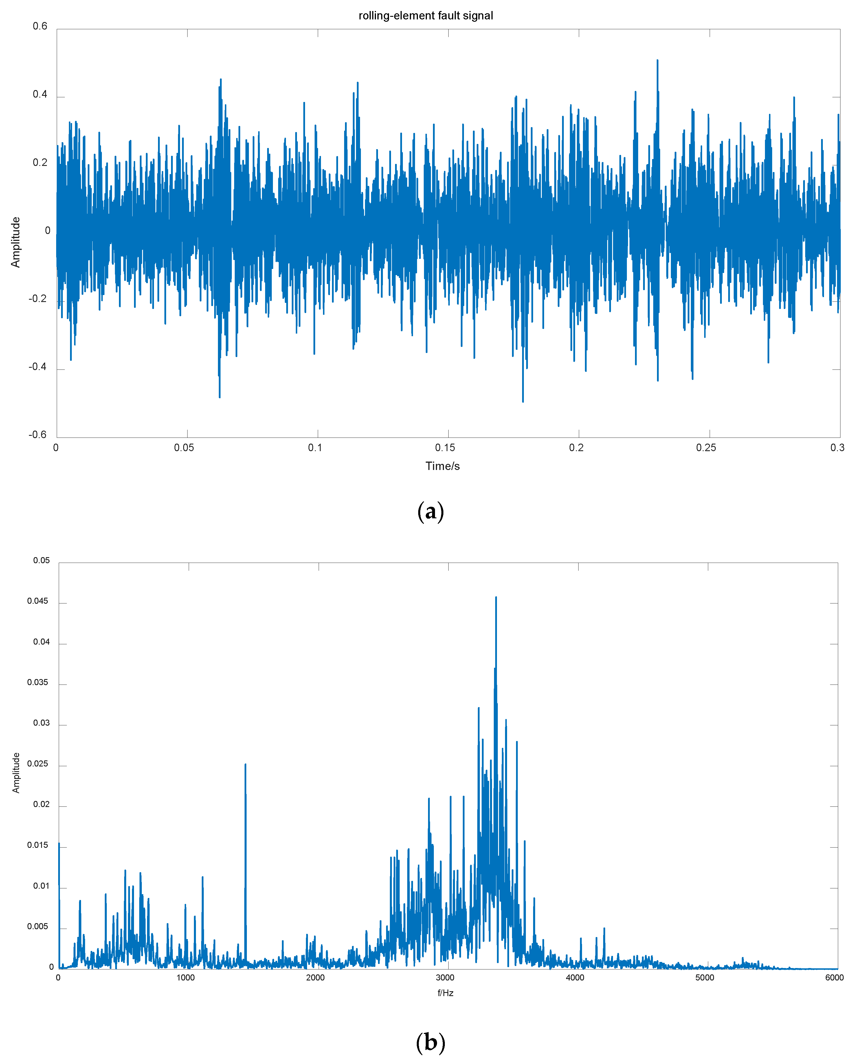
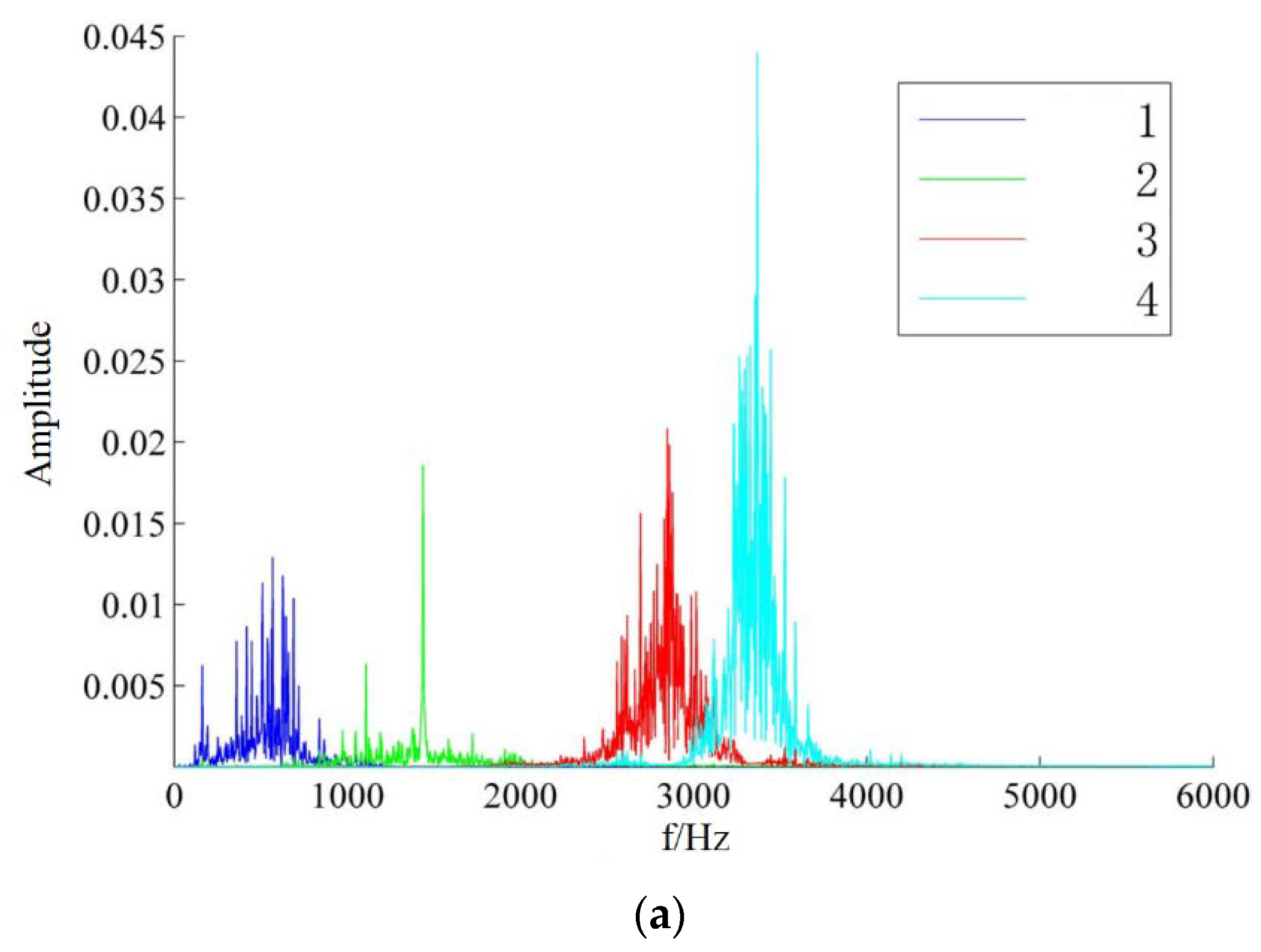
When cracks or other faults occur in the components of the rolling bearing, the vibration state of the rolling bearing will change. In order to accurately analyze the characteristic information contained in the vibration signal, this paper uses the rolling-element fault data with a motor speed of 1797 rpm and a damage diameter of 0.1778 mm, and was compared with several commonly used optimization algorithms which include Particle Swarm Optimization (PSO), Genetic Algorithm (GA), and BSO.
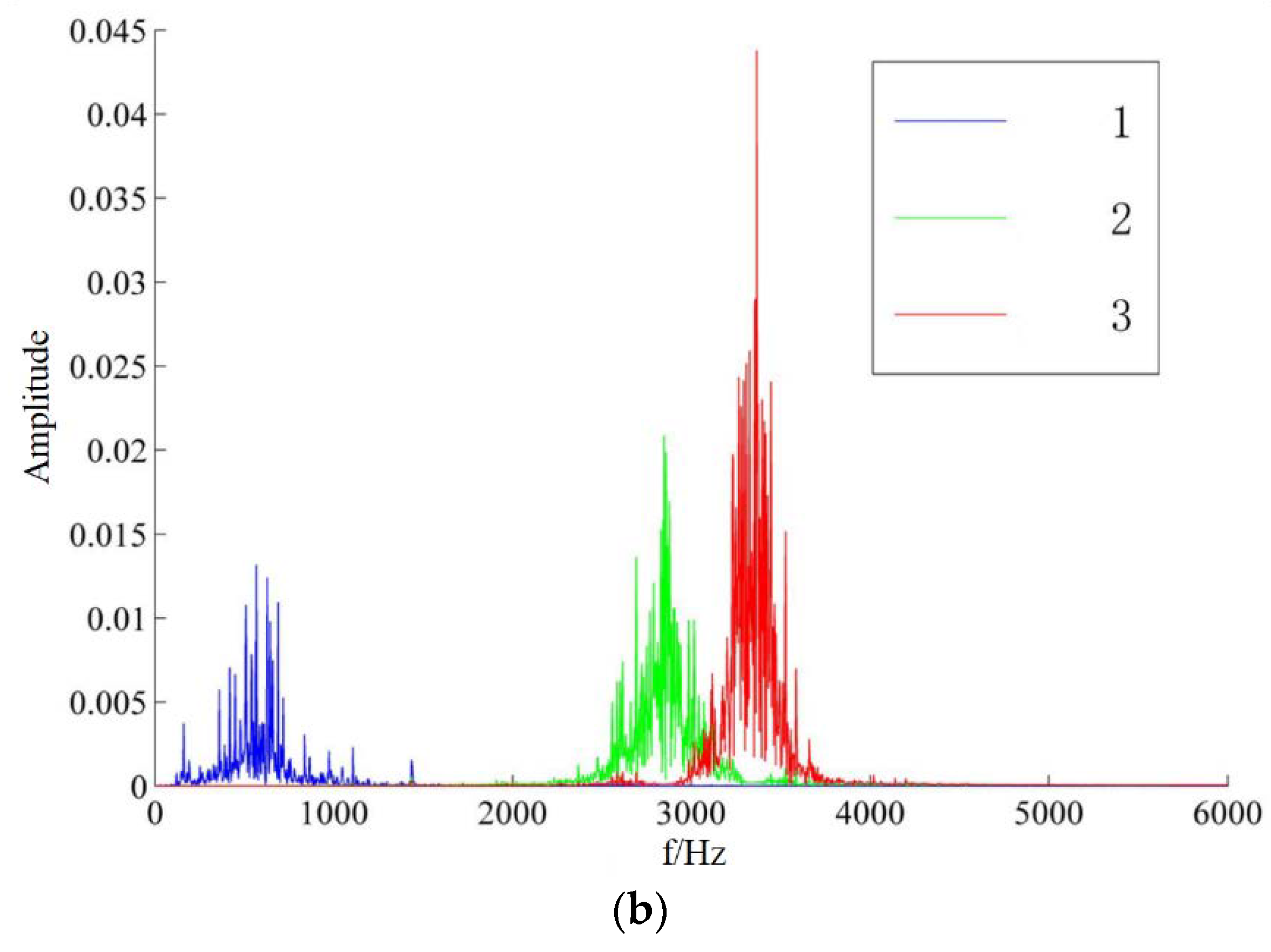
From Figure 2b, it can be seen that the fault signal mainly includes 3 main frequency components.
The parameter settings of the PSDMBSO algorithm were divided into BSO parameter settings and update, and initialization parameter settings. The BSO parameters were the same as in Reference [22], the initialization parameters (m, n, etc.) were set to common values, and the update parameters were selected from the optimal values in 10 random parameter experiments within the common range. Update and initialization parameters according to the final results of the simulation experiment are shown in Table 2.
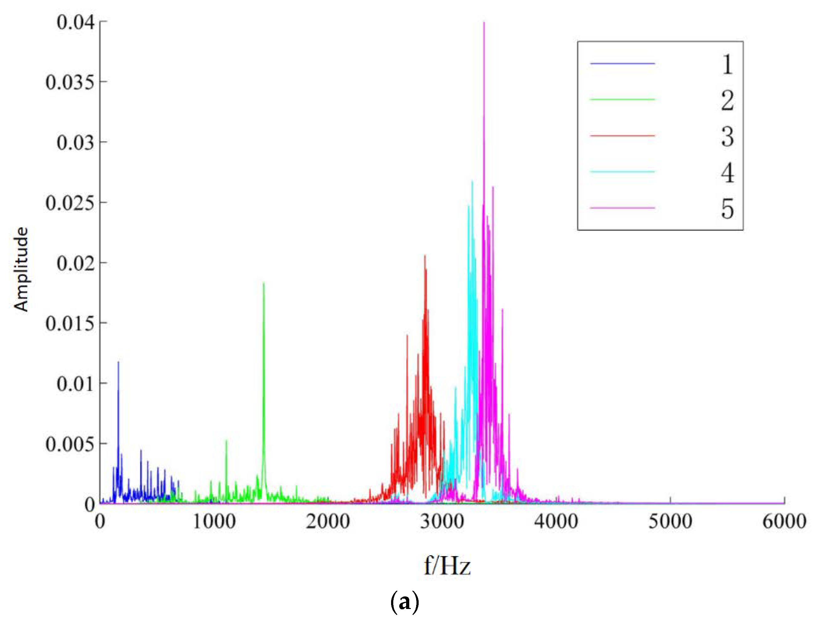
According to Konstantin Dragomiretskiy’s documents, the parameters that the VMD algorithm needs to be determined are: the number of IMF components K , penalty factor α , convex function optimization-related parameter t a u , center frequency initialization setting i n i t , center frequency update related parameter D C , termination condition ε . Parameters other than K and α have little effect on the decomposition effect, set to common values, namely, t a u = 0 , i n i t = 1 , D C = 0 , ε = 1 e 7 . The spectral distribution diagrams of the modal components are shown in Figure 3 and Figure 4.
It can be seen from Figure 3a,b that the original signal is decomposed into 5 and 4 modal components, respectively, and different numbers of false components appear; that is, the over-decomposition phenomenon occurs.
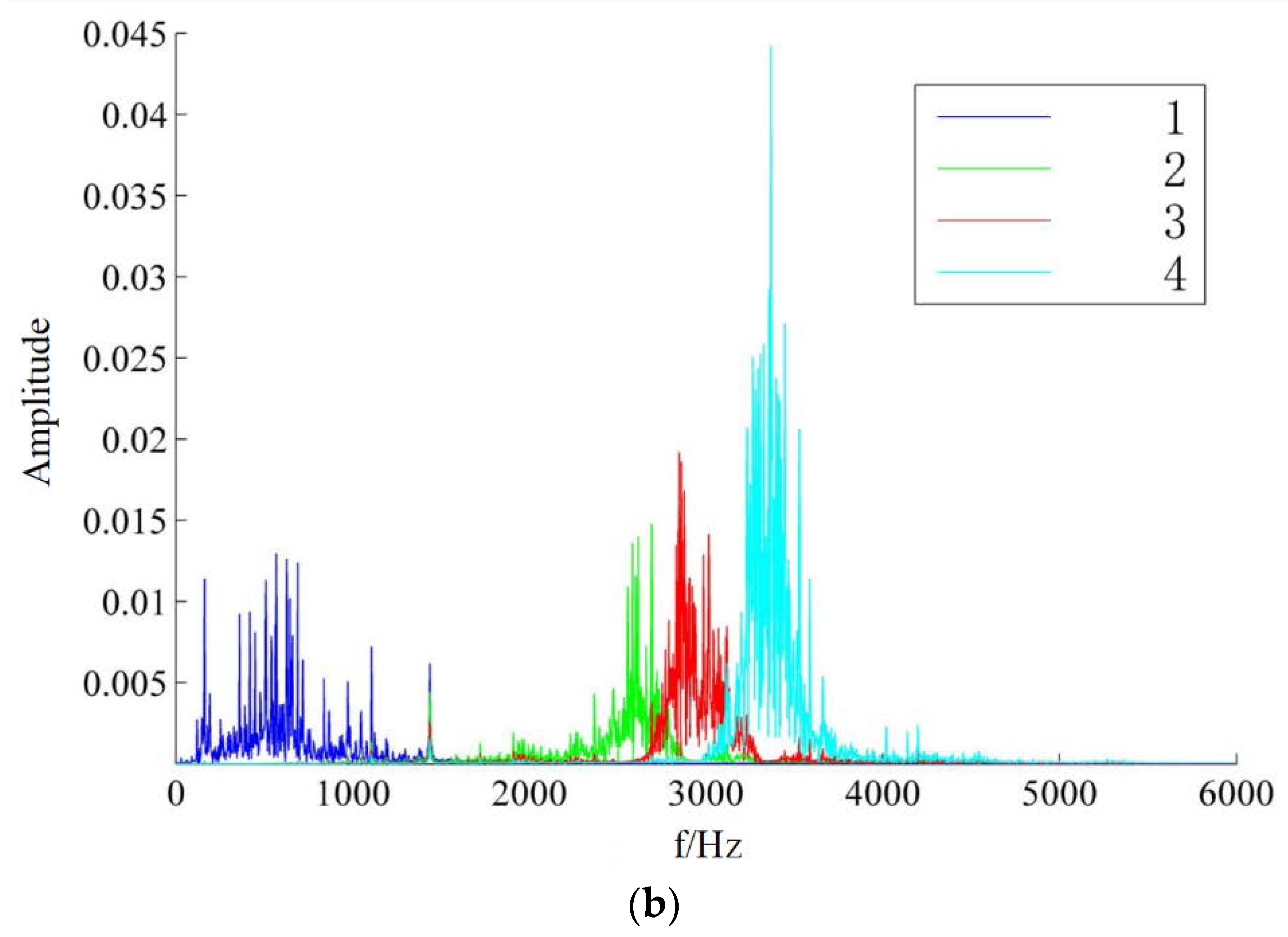
It can be seen from Figure 4b that the original signal is decomposed into 4 modal components, while the result of the algorithm we proposed is 3 modal components, and there is no modal aliasing phenomenon, indicating that the original signal achieves a better good decomposition effect.
In order to get close to the actual situation, we used the bearing failure data from the Bearing Data Center of Western Reserve University. The set load was 2 Hp, which means the speed was 1750 r/min. By compressing the obtained time–frequency diagram to a resolution of 64 × 64 in the same proportion, 7000 training set images and 1000 test set images were finally obtained. The specific fault types are shown in Table 3. For the four categories of vibration acceleration signals of ten types of faults at rated power, the optimal parameter combinations searched by the PSDMBSO algorithm are shown in Table 4 below.

3.2. Improved Filter Construction Based on Band Entropy

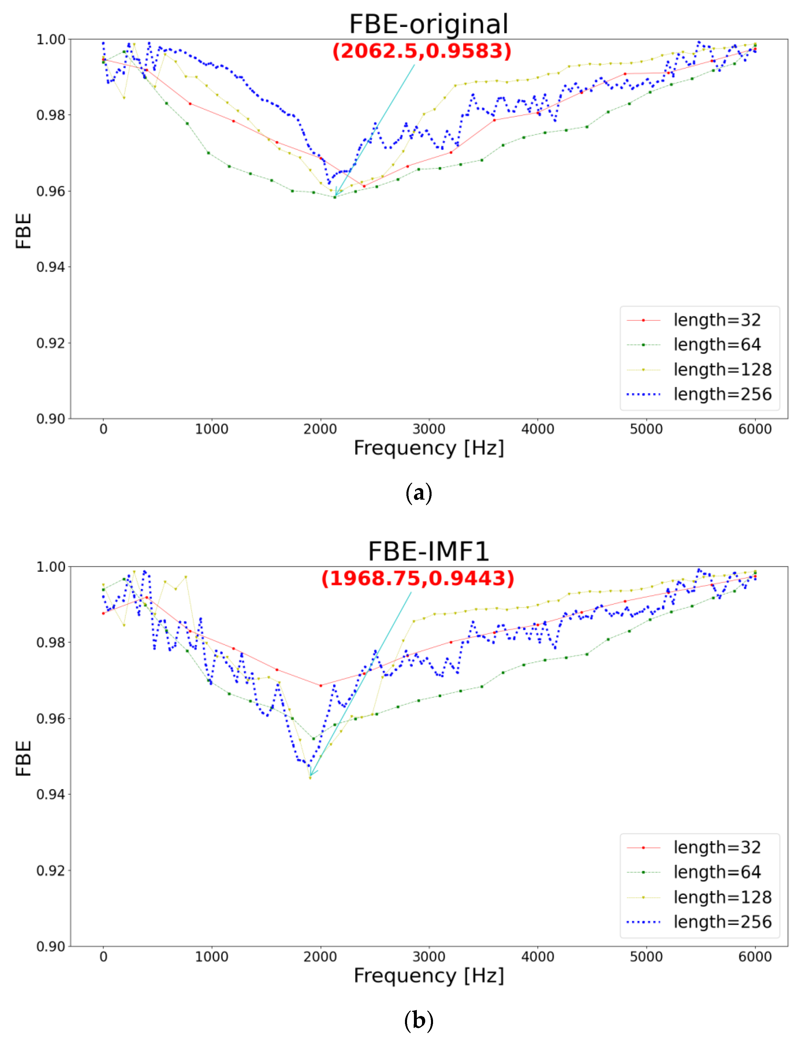
Take rolling bearing load 2 Hp, damage radius 0.1778 mm, speed 1750 r/min, sampling frequency 12 kHz inner-ring fault data as an example. The final selection results of reconstruction components are as follows: the frequency band entropy data of the original signal under window functions of different lengths is shown in Figure 5a below.
It can be seen that the center frequency is 2062.5 Hz, and the corresponding optimal window function length is 64. According to the above formula, the pass band of the corresponding band filter of the original signal can be obtained as [1921.375, 2203.625]. In addition, the parameters obtained by the PSMBSO algorithm optimization are K = 8 , α = 249 
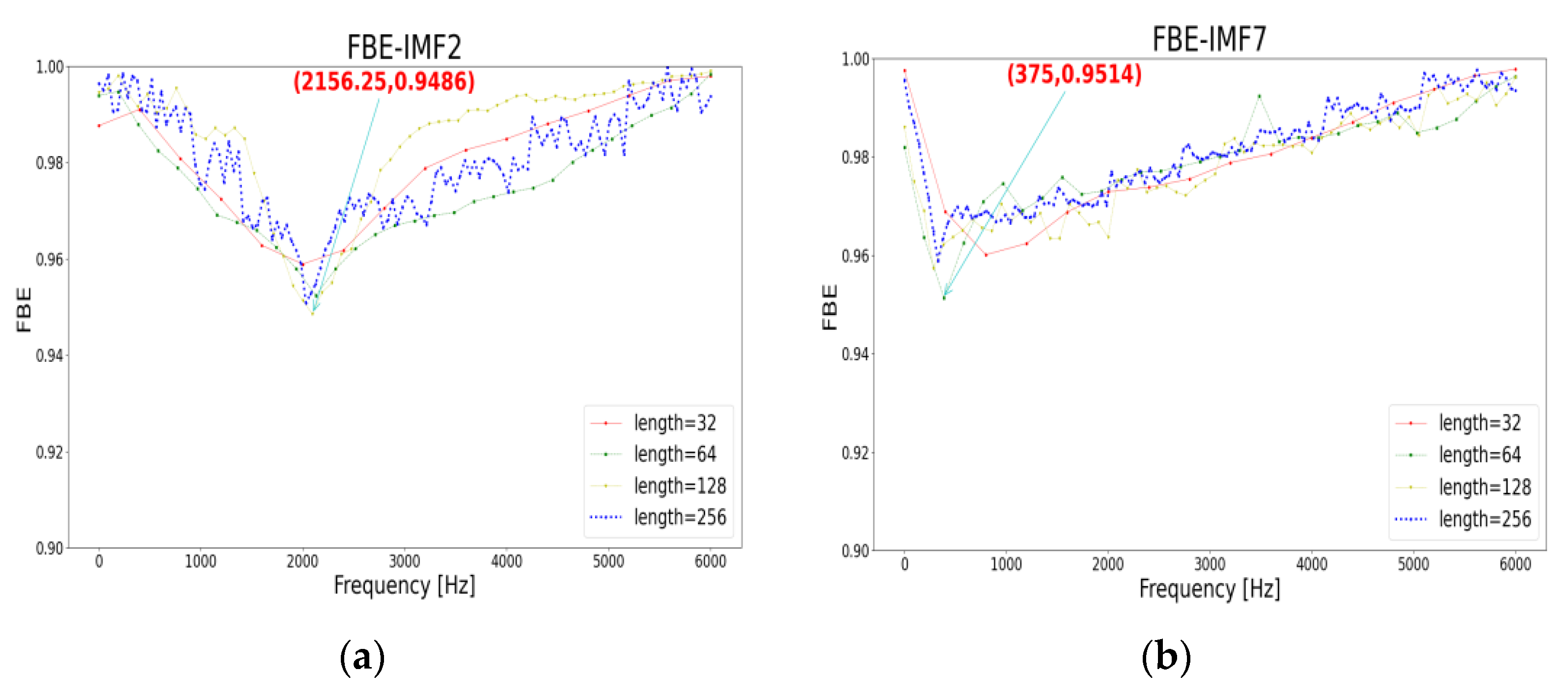
, and then the corresponding IMF components can be obtained, and the same operation is performed on each component. The final result is that IMF1 and IMF2 are selected as the optimal reconstruction components. The detailed process is as follows: as shown in Figure 5b and Figure 6a, the corresponding center frequency and optimal window function length can be obtained as [1968.75, 128] and [2156.25, 128]. According to the formula, the final corresponding filters are [1898.4375, 2037.0625] and [2085.9375, 2226.5625], which meets the previously proposed standards, and the remaining components do not meet the requirements, so they are discarded. Take IMF7 as an example—its center frequency is 375 Hz, the corresponding optimal window function length is 64, and the final result is [234.375,515.625], which obviously does not meet the requirements. The detailed results are shown in Figure 6b below.

3.3. Experimental Result

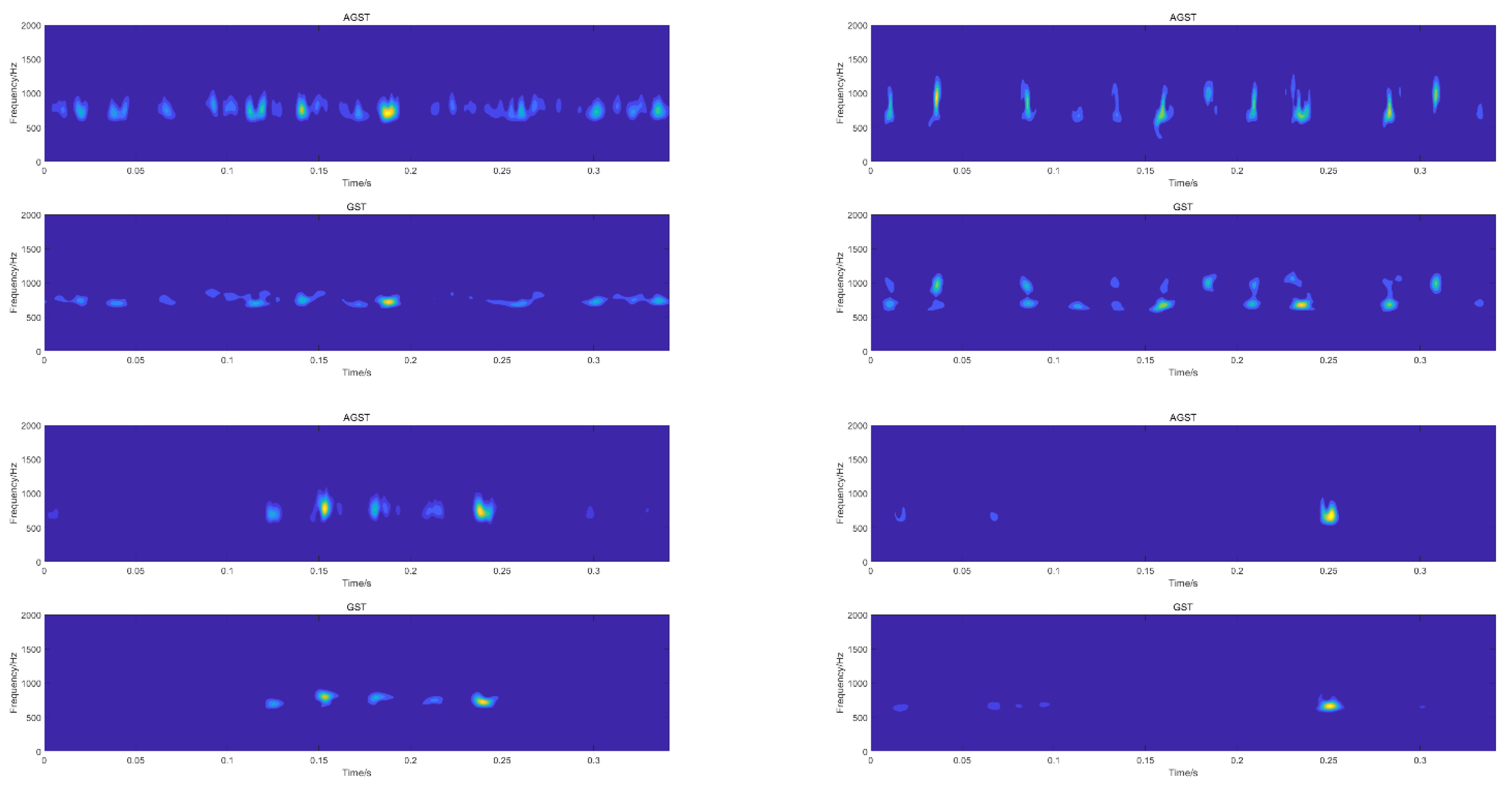
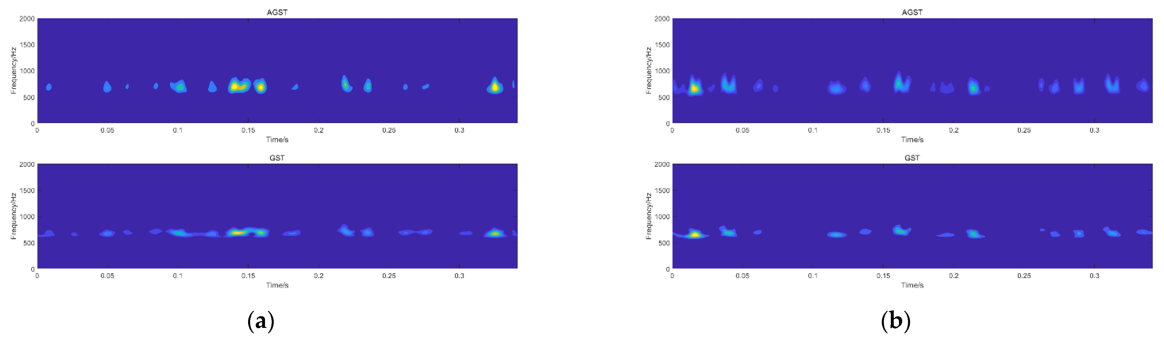
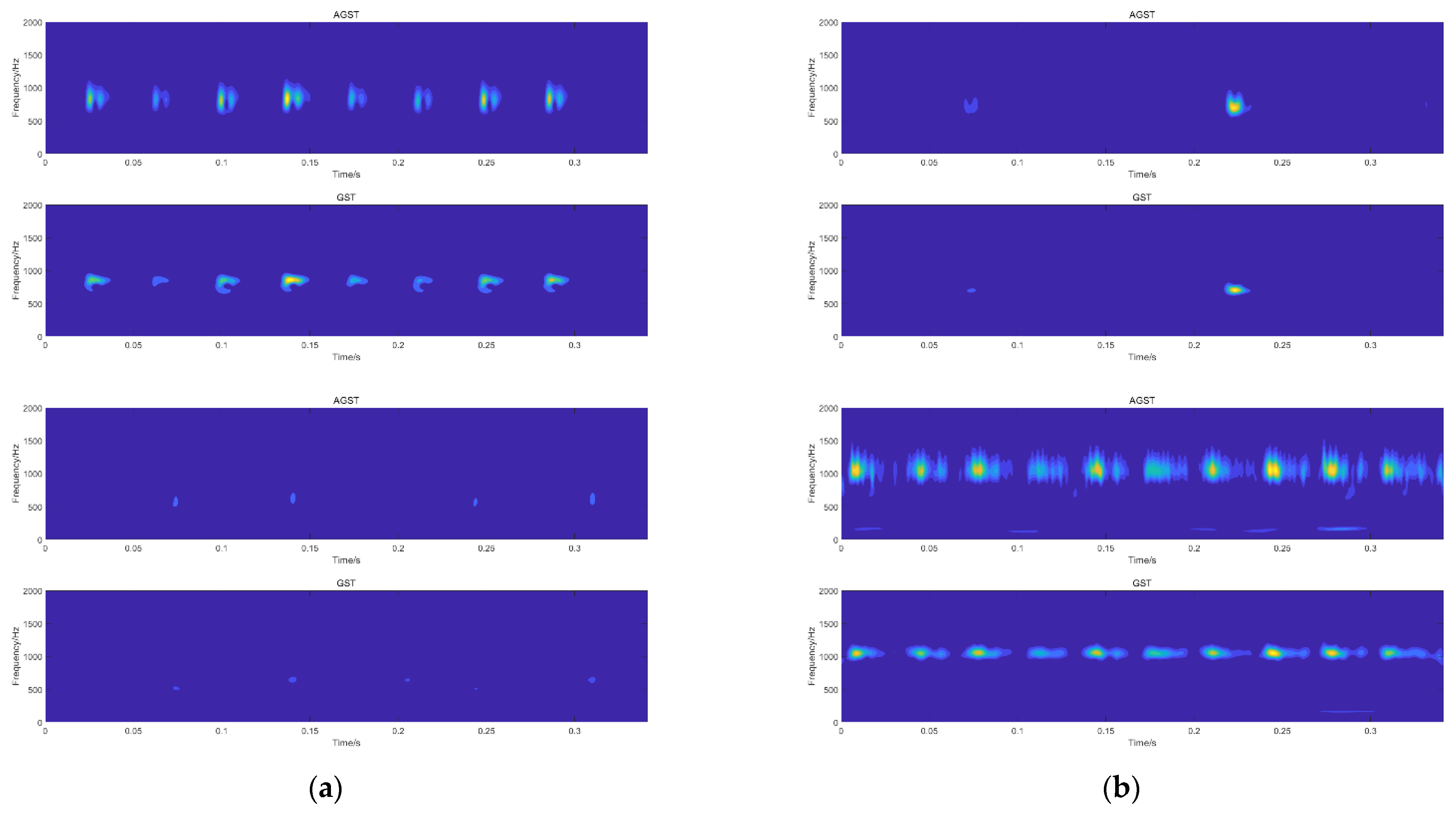
In this paper, the bearing fault data set of the drive end was selected, and the one-dimensional signal was converted into a time–frequency map using AGST transformation on the reconstructed signal. At the same time, the time–frequency map was compared with the time–frequency map processed by GST, as shown in Figure 7 and Figure 8.
The upper part of Figure 8b is the outer-ring fault data with the fault diameter equal to 0.5334 mm, and the lower part is the normal signal.
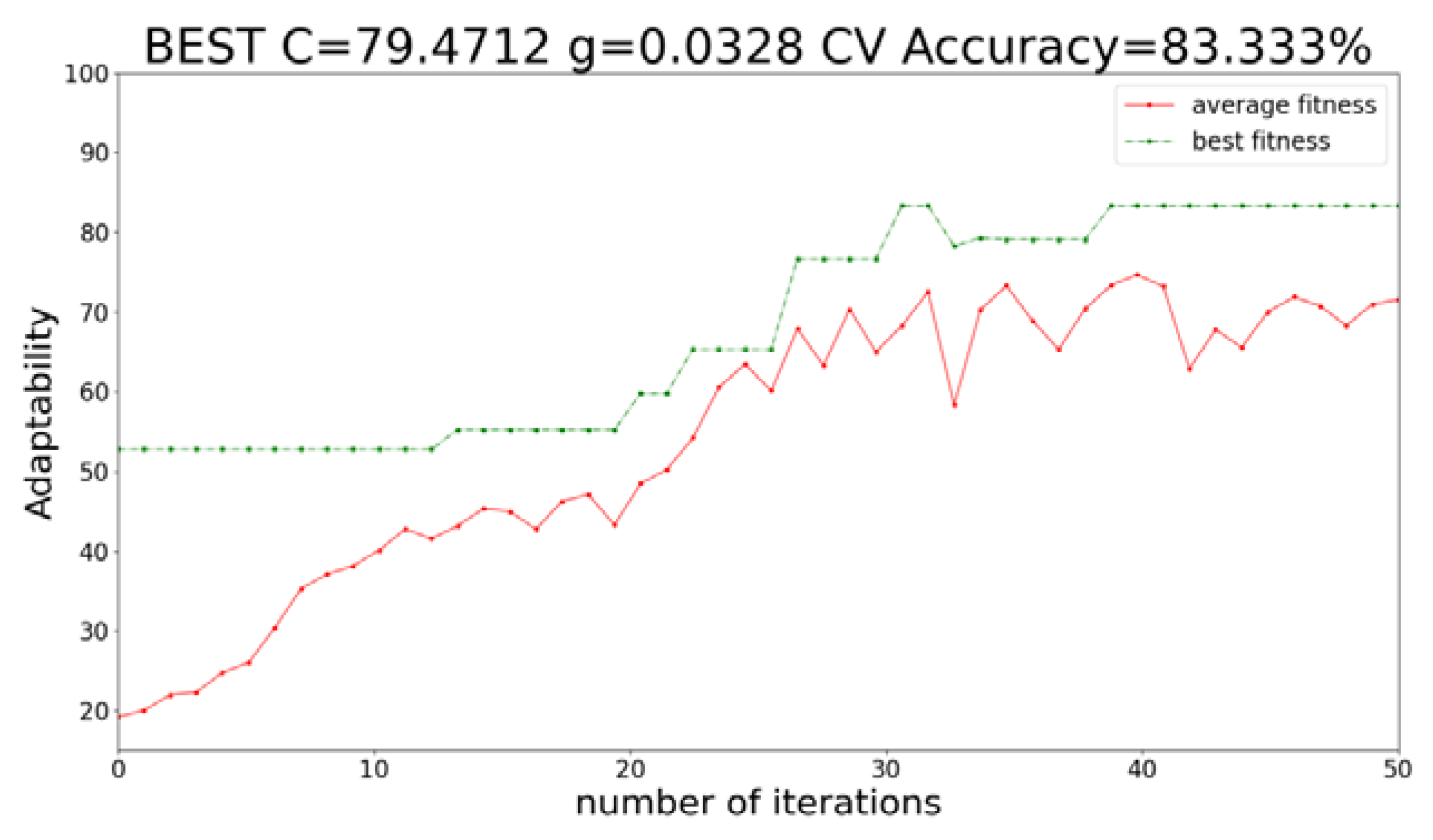
For the optimization problem of SVM, the fitness function was selected as the 5-fold cross-validation method. When the accuracy rate reaches the highest and does not change, the corresponding C and g are the best parameters. In this paper, the range of C and g was set to 0–100.
As shown in Figure 9, the blue curve represents the average fitness, and the red curve represents the best fitness. With the increase of the number of iterations, the red best fitness curve shows an upward trend, and reaches the maximum when the number of iterations reaches 30. Excellent and remaining unchanged, the correct rate of 5-fold cross-validation is 83.333%, the best parameter C = 79.4712, the best parameter g = 0.0328, and the SVM classification model is established with these two parameters.
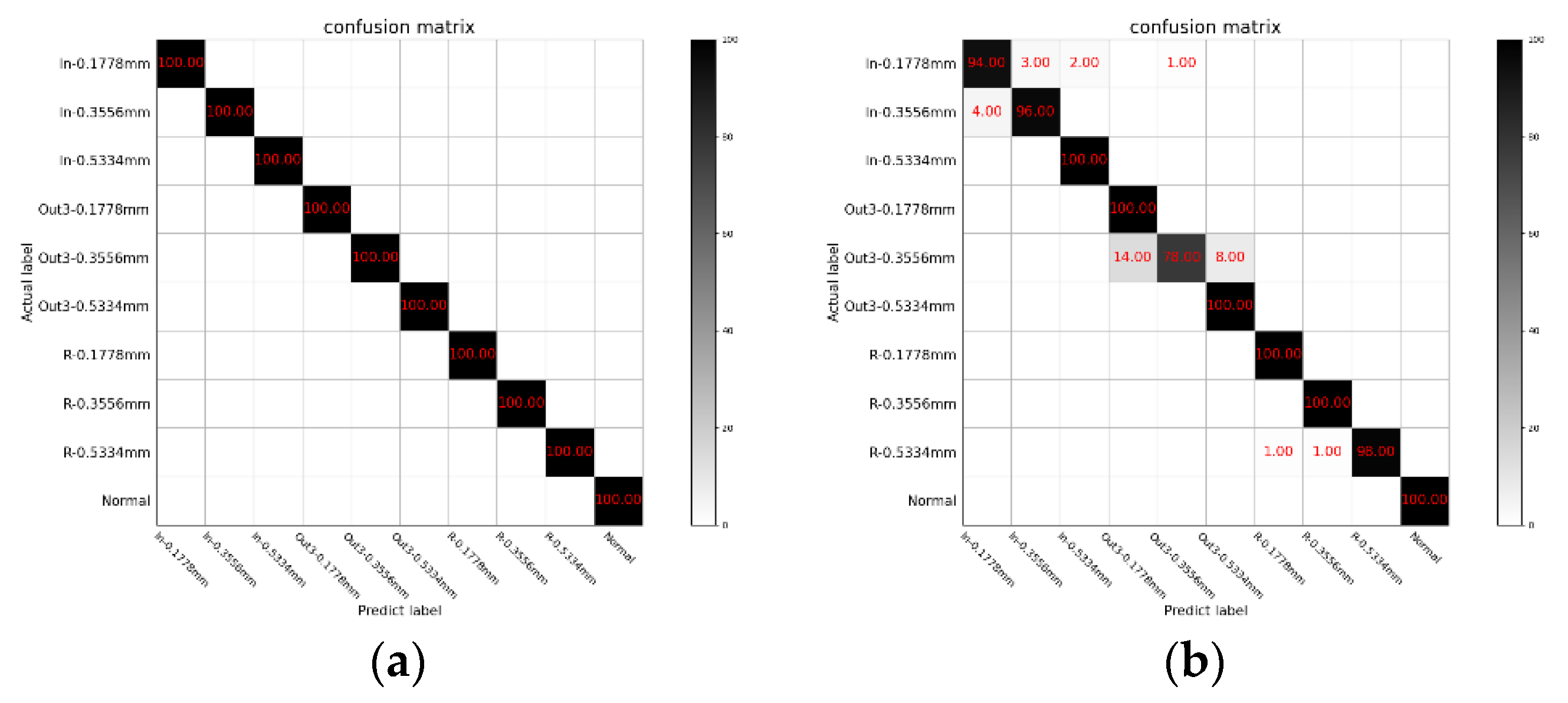
The optimized SVM model was selected, and the experimental results are shown in Figure 10a.
It can be seen from Figure 10a that the predicted label and the actual label of the test set completely overlap, which means the diagnosis accuracy of the bearing reaches 100%.
We selected the same data, used the Generalized S-Transform to convert the reconstructed signal into a time–frequency map, and other steps are the same. The final test set result is shown in 
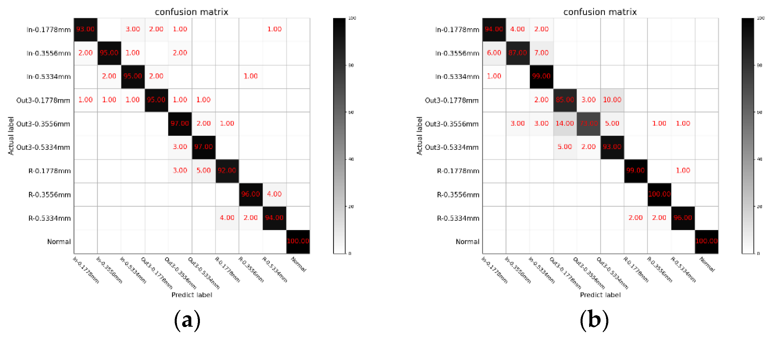
Figure 10b. Under the same data, the final result of using improved screening criteria is shown in Figure 11a.
It can be drawn from Figure 10b that the final result of using the Generalized S-Transform is 96.6%, which shows the superiority of AGST. Compared with the method, the accuracy of the diagnostic model we proposed is improved by 3.4% at rated power. As shown in Figure 11a, the accuracy of the test set is 95.4%, which is also 4.6% lower than the method we proposed, which illustrates the effectiveness of the screening criteria we proposed. In order to further address the advantages of the feature extraction method we proposed, we used the traditional VMD decomposition method ( K = 6 , α = 2000 ) to decompose the signal, and then used the same processing.
It can be seen from Figure 11b that the accuracy is 92.60%. Under the same data, the method we proposed has an accuracy rate of 7.40% higher compared with the traditional VMD, which shows that the method we proposed can accurately identify different faults with the same damage diameter.
Based on the above comparative experiments, the fault diagnosis results of the above methods for different positions and different degrees of damage under the rated power are further explored. The method we proposed is named Method 1. The method that uses PSDMBSO to optimize the VMD parameter + optimized band filters + AGST + CNN + Softmax is named Method 2. The method that PSDMBSO-optimized VMD + unoptimized band filters + AGST + SVM is named Method 3. The method that uses the traditional VMD decomposition method is named Method 4.
The network structure and parameters of CNN in Method 2 are the same as in Method 1, the SVM parameters C and g in Method 3 are randomly selected parameters, and the parameter of traditional VMD in Method 4 was set to [6, 2000].
In order to further test the diagnostic accuracy of method we proposed under non-rated power, the data under the same state were selected for experimental comparison. The final results are shown in Table 5, Table 6 and Table 7.
It can be seen that the method we proposed has an accuracy close to 100%. Compared to other methods with better current-level effects, the accuracy rate has been improved by 6.2–8.9%. The result shows that the method we proposed is suitable for the complex and changeable working environment of the rolling bearing, which has extraordinary significance for the diagnosis of rolling bearings in practical applications.
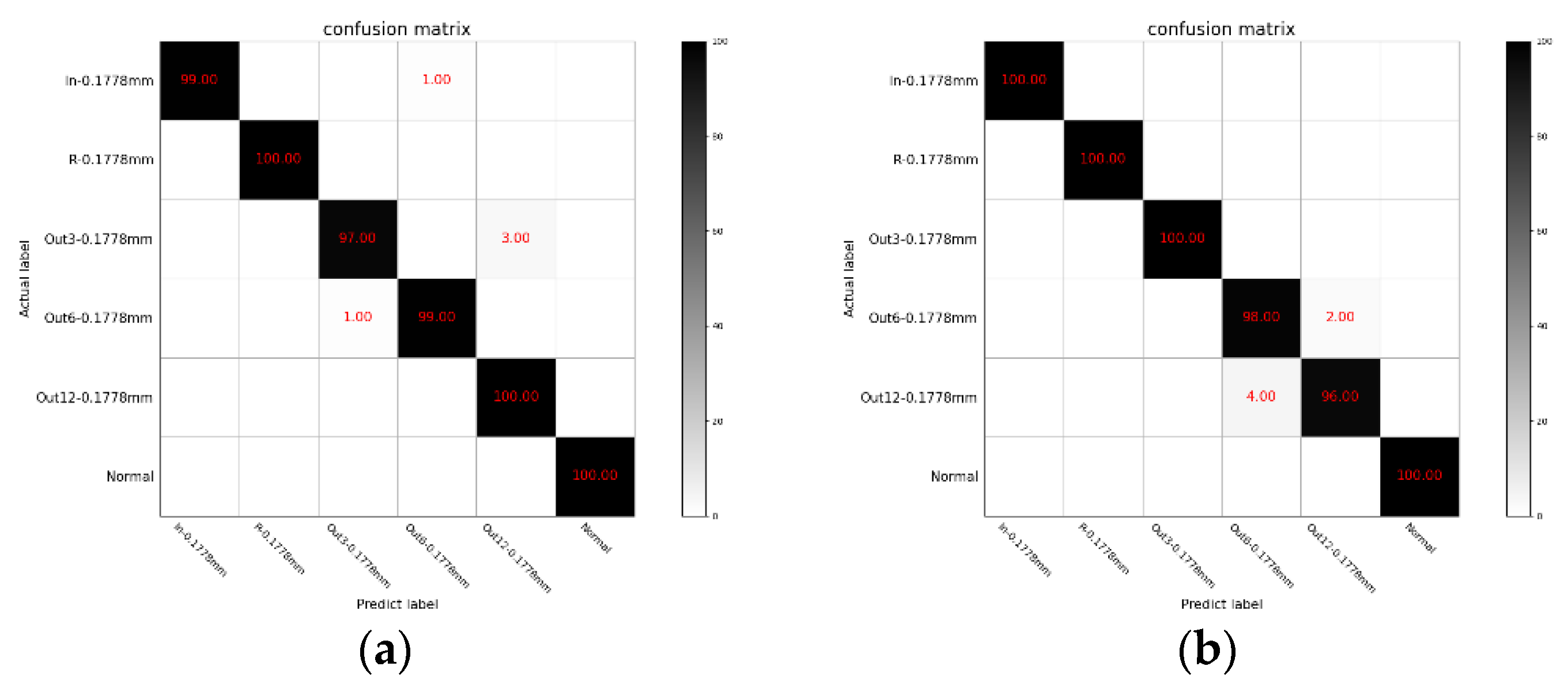
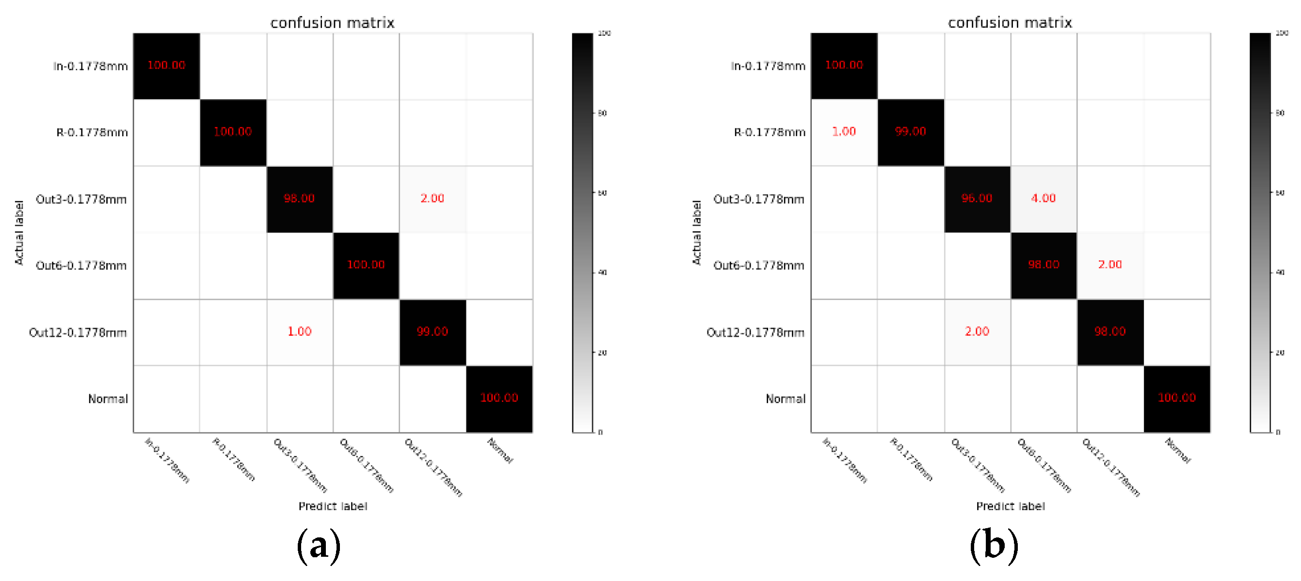
In order to further verify the effectiveness of the method we proposed in dealing with minor faults, we selected 100 groups of fault data (0.1778 mm) in different load states, totaling 2400 test samples. First, the micro faults under different load conditions were tested separately, and the results are shown in Figure 12 and Figure 13. Finally, the experimental results corresponding to different loads are shown in Table 8.
It can be seen from Table 8 that the method we proposed has a higher accuracy in the identification of minor faults than the other three methods. At the same time, it can be seen from the table that compared with the other three methods, the accuracy rate of the method we proposed can still remain above 96% when judging the three precise fault types that belong to the same minor fault type of the outer ring, but the fault location is different. This greatly improves the accurate judgment of minor faults required in actual production.
In order to further explore the real anti-noise performance of the method we proposed in the actual working environment, we introduced the standard noise library NOISEX-92 in the Signal Processing Information Base (SPIB). The noise data in the library were all collected under the condition of a sampling frequency of 19.98 KHz, and the duration was 235 s. By changing the sampling frequency of the noise signal to 12 KHz, the frequency calibration of the noise signal and the fault signal was completed, and on this basis, the calibrated noise signal was added to the original vibration signal. The experimental results are shown in Table 9.
As shown in Table 9, the difference between Method 1 and Method 2 is the signal–image processing method. From the result, we can see that the lowest value of Method 1 is higher than the highest value of Method 2, which shows that the Adaptive Generalized S-Transform we proposed improves noise immunity by extracting more effective features. Comparing Method 1 and Method 3, we can see that our proposed reconstruction component selection criterion improves the anti-interference ability of the whole model by removing the interference components and extracting more fault features. In summary, the method we proposed has been maintained at a higher level and the average accuracy rate is also 7.61–9.60% higher than other methods in the table, which shows that the fault diagnosis method we proposed can better separate fault and noise components.

3.4. Discussion of Experimental Results

As can be seen from Table 5, Table 6 and Table 7, with the deepening of the fault degree (damage diameter), the diagnostic accuracy of the four models is increasing. For faults at different positions with a fault diameter of 0.1778 mm, the accuracy of the method we proposed can reach more than 97%, which is 5–8% higher than the other three models, which shows that the method we proposed has improved the recognition accuracy of minor faults in the case of different fault degrees.
It can be seen from further experiments on different fault types under minor faults that the recognition accuracy of the model we proposed is 0.73–1.4% lower than that of general faults, while the other three models have more than 2%, which shows that the method has strong adaptability to fault identification of different fault degrees. At the same time, it can be seen from the comparative test results under minor faults that the method we proposed enhances the sensitivity of the diagnostic model to minor faults.
Judging from the noise experiment under minor faults, compared with the accuracy rate of the other three models below 92%, the accuracy rate of the diagnostic model we proposed is maintained at about 98%, which shows that the parameter optimization and AGST can extract the more effective fault features and thus improve the diagnostic accuracy in noisy environments.

4. Conclusions

A rolling bearing fault diagnosis method based on parameter optimization and AGST was proposed. Compared with the traditional VMD methods, the fault diagnosis method we proposed achieves higher fault diagnosis accuracy through more comprehensive and accurate feature extraction under general failure. For minor faults, the diagnostic accuracy rate of our proposed method can still remain above 98.5% compared with other methods under different loads, which is 5.17–9.5% higher than other methods. The diagnostic accuracy of our proposed method can still be maintained above 97.96% when some types of noise exist. Comprehensive experimental results show that the diagnostic method proposed by us significantly improves the diagnostic accuracy and anti-interference ability of rolling bearings by realizing accurate and comprehensive extraction of fault features.

Author Contributions

Conceptualization, Y.P.; methodology, Y.P.; software, Y.P.; validation, Y.P.; formal analysis, Y.P.; investigation, Y.P.; resources, Y.P. and X.M.; data curation, Y.P.; writing—original draft preparation, Y.P.; writing—review and editing, Y.P. and X.M.; visualization, Y.P.; supervision, X.M.; project administration, X.M. All authors have read and agreed to the published version of the manuscript.

Funding

This research was funded by the National Key R&D Program of China under Grant number 2020YFB2007700.

Institutional Review Board Statement

Not applicable.

Informed Consent Statement

Not applicable.

Data Availability Statement

The data that support the findings of this study are from the data source of Case Western Reserve University’s Electrical Engineering Laboratory for simulation experiments.

Conflicts of Interest

The authors declare no conflict of interest.

References

  1. Berredjem, T.; Benidir, M. Bearing faults diagnosis using fuzzy expert system relying on an improved range overlaps and similarity method. Expert Syst. Appl. 2018, 108, 134–142. [Google Scholar] [CrossRef]
  2. Xu, T.L.; Chen, W.Q. Research of Rolling Bearing Fault Diagnosis Based on Expert System. Coal Mine Mach. 2010, 11, 234–236. [Google Scholar]
  3. Song, X.J.; Zhao, W.X. A Review of Rolling Bearings Fault Diagnosis Approaches Using AC Motor Signature Analysis. In Proceedings of the CSEE 2021, Lisbon, Portugal, 21–23 June 2021; pp. 1–15. [Google Scholar]
  4. Jiang, H.Y. Fault Diagnosis of Rolling Element Bearing Based on Normal Distribution Model Parameters and LS-SVM. Tech. Autom. Appl. 2019, 38, 11–16. [Google Scholar]
  5. Zhang, M.D.; Lu, J.H.; Ma, J.H. Fault Diagnosis of Rolling Bearing Based on Multi-Scale Convolution Strategy CNN. J. Chongqing Univ. Technol. (Nat. Sci.) 2020, 34, 102–110. [Google Scholar]
  6. Meng, Z.; Guan, Y.; Pan, Z.Z. Fault Diagnosis of Rolling Bearing Based on Secondary Data Enhancement and Deep Convolution Network. J. Mech. Eng. 2022, 1, 13. [Google Scholar]
  7. Lai, H.Y. A rolling bearing fault diagnosis method based on deep neural network. Min. Technol. 2020, 20, 131–134. [Google Scholar]
  8. Sha, M.Y.; Liu, L.G. Summary of bearing fault diagnosis technology based on vibration signal. Bearings 2015, 430, 59–63. [Google Scholar]
  9. Cheng, J.S.; Yu, D.J.; Yang, Y. Fault diagnosis method based on intrinsic mode singular value decomposition and support vector machine. Acta Autom. Sin. 2006, 3, 475–480. [Google Scholar]
  10. Li, L.Q.; Liu, Y.Q.; Liao, Y.Y. MCKD Fault Diagnosis Method for Bearing Based on Particle Swarm Optimization. Bearing 2020, 6, 45–50. [Google Scholar]
  11. Tong, Z.J.; Lu, T.; Qin, Z.N. Fault diagnosis of rolling bearing based on PSO-VMD and Bayesian network. J. Henan Univ. Technol. (Nat. Sci. Ed.) 2021, 40, 95–104. [Google Scholar]
  12. Hua, L. An optimized VMD method and its applications in bearing fault diagnosis. Measurement 2020, 166, 108185. [Google Scholar]
  13. Liu, J.C.; Quan, H.; Yu, X. Rolling bearing fault diagnosis based on parameter optimization VMD and sample entropy. Acta Autom. Sin. 2021, 1, 12. [Google Scholar]
  14. Tang, G.J.; Wang, X.L. Parameter Optimized Variational Modal Decomposition Method with Application to Incipient Fault Diagnosis of Rolling Bearings. J. Xi’an Jiaotong 2015, 49, 73–81. [Google Scholar]
  15. Liu, T.; Chen, J.; Dong, G. The fault detection and diagnosis in rolling element bearings using frequency band entropy. Proc. Inst. Mech. Eng. Part C J. Mech. Eng. Sci. 2013, 227, 87–99. [Google Scholar] [CrossRef]
  16. Cao, S.; Xu, F.; Ma, T. Fault diagnosis of rolling bearing based on multiscale one-dimensional hybrid binary pattern. Measurement 2021, 181, 109552. [Google Scholar] [CrossRef]
  17. Zheng, Z.; Zhang, H.Q.; Pan, Y. Rolling bearing Fault diagnosis based on IWOA-LSTM. J. Vib. Shock. 2021, 40, 274–280. [Google Scholar]
  18. Xiao, X.; Wang, J.X.; Zhang, Y.J. A Two-dimensional Convolutional Neural Network Optimization Method for Bearing Fault Diagnosis. Proc. CSEE 2019, 39, 4558–4568. [Google Scholar]
  19. Shao, H.D. Fault Diagnosis of a Rotor-Bearing System Under Variable Rotating Speeds Using Two-Stage Parameter Transfer and Infrared Thermal Images. IEEE Trans. Instrum. Meas. 2021, 70, 3524711. [Google Scholar] [CrossRef]
  20. Luo, J.H.; Huang, G.Y. Check valve fault diagnosis based on generalized S-transform and deep confidence network. J. Electron. Meas. Instrum. 2019, 33, 192–198. [Google Scholar]
  21. Shi, Y. Brain storm optimization algorithm. In International Conference in Swarm Intelligence; Springer: Heidelberg, Germany, 2011; pp. 303–309. [Google Scholar]
  22. Yang, Y.T.; Shi, Y.H.; Xia, S.R. Discussion mechanism based brain storm optimization algorithm. J. Zhejiang Univ. Eng. Ed. 2013, 47, 1705–1711. [Google Scholar] [CrossRef]
Figure 1. Diagnosis model structure diagram.
Machines 10 00207 g001
Figure 2. (a) The time domain diagram of the signal; (b) signal spectrogram of the signal.
Machines 10 00207 g002
Figure 3. (a) Optimization result of BSO algorithm; (b) optimization result of PSO algorithm.
Machines 10 00207 g003aMachines 10 00207 g003b
Figure 4. (a) Optimization result of GA; (b) optimization result of PSDMBSO.
Machines 10 00207 g004aMachines 10 00207 g004b
Figure 5. (a) Frequency band entropy of inner-ring fault signal; (b) frequency band entropy of IMF1.
Machines 10 00207 g005
Figure 6. (a) Frequency band entropy of IMF2; (b) frequency band entropy of IMF7.
Machines 10 00207 g006
Figure 7. (a) Time–frequency diagram of rolling-element fault signal; (b) time–frequency diagram of inner-ring fault signal.
Machines 10 00207 g007aMachines 10 00207 g007b
Figure 8. (a) Time–frequency diagram of outer-ring fault signal; (b) time–frequency diagram of normal signal.
Machines 10 00207 g008
Figure 9. The process of SVM parameter optimization.
Machines 10 00207 g009
Figure 10. (a) Test sample confusion matrix diagram(AGST); (b) test sample confusion matrix diagram(GST).
Machines 10 00207 g010
Figure 11. (a) Test sample confusion matrix diagram(unimproved FBE); (b) test sample confusion matrix diagram(traditional VMD).
Machines 10 00207 g011
Figure 12. (a) The result of 0 Hp-1797 r/min; (b) the result of 1 Hp-1772 r/min.
Machines 10 00207 g012
Figure 13. (a) The result of 2 Hp-1750 r/min; (b) the result of 3 Hp-1730 r/min.
Machines 10 00207 g013
Table 1. Neural network model parameters.
Serial NumberNetwork LayerConvolution Kernel SizeNumber of Convolution Kernels
C1Convolutional layer 13 × 38
S2Maximum pooling layer 12 × 21
C3Convolutional layer 23 × 316
S4Maximum pooling layer 22 × 21
Table 2. PSMBSO algorithm parameter settings.
VariablesNumerical ValuesVariablesNumerical Values
n100 p c e n s 0.7
m5 N m i 2000
D2 N m t 10
p D i s 0.2 p r p 0.95
p c e n 0.6 c g min 1.5
p r g 0.98 c g max 3
c 1 p min 1 p p e r 0.08
c 1 p max 1.5 η 0.05
c 2 p min 1 α 0.01
c 2 p max 2 β 0.005
Table 3. Types of rolling bearing failure.
Bearing StatusLabels
Inner-ring failure-0.1778 mm0
Inner-ring failure-0.3556 mm1
Inner-ring failure-0.5334 mm2
Outer-ring failure (3 o’clock)-0.1778 mm3
Outer-ring failure (3 o’clock)-0.3556 mm4
Outer-ring failure (3 o’clock)-0.5334 mm5
Rolling-element failure-0.1778 mm6
Rolling-element failure-0.3556 mm7
Rolling-element failure-0.5334 mm8
normal status9
Table 4. Types of rolling bearing failure optimal parameter combination [ K , α ].
Bearing StatusLabels
normal status[7, 2064]
Inner-ring failure-0.1778 mm[8, 249]
Inner-ring failure-0.3556 mm[3, 1986]
Inner-ring failure-0.5334 mm[6, 2022]
Outer-ring failure (3 o’clock)-0.1778 mm[5, 2008]
Outer-ring failure (3 o’clock)-0.3556 mm[4, 1498]
Outer-ring failure (3 o’clock)-0.5334 mm[8.1021]
Rolling-element failure-0.1778 mm[3, 2478]
Rolling-element failure-0.3556 mm[4, 1489]
Rolling-element failure-0.5334 mm[13, 2230]
Table 5. Experimental comparison results with a load of 0 Hp.
Fault LocationDamage Diameter (mm)Method 1Method 2Method 3Method 4
Inner-ring failure0.177899909289
0.3556100919492
0.5334100949694
Outer-ring failure (3 o’clock)0.1778100919392
0.355699929490
0.5334100929593
Rolling-element failure0.1778100909490
0.3556100929491
0.5334100939591
normalNONE100100100100
Average classification accuracy99.892.594.792.0
Table 6. Experimental comparison results with a load of 1 Hp.
Fault LocationDamage Diameter (mm)Method 1Method 2Method 3Method 4
Inner-ring failure0.1778100909190
0.3556100919289
0.5334100929491
Outer-ring failure (3 o’clock)0.177897909391
0.3556100899090
0.5334100939691
Rolling-element failure0.1778100909389
0.3556100919490
0.533498.5929291
normalNONE100100100100
Average classification accuracy99.791.893.591.2
Table 7. Experimental comparison results with a load of 3 Hp.
Fault LocationDamage Diameter (mm)Method 1Method 2Method 3Method 4
Inner-ring failure0.177899909190
0.3556100919289
0.5334100899493
Outer-ring failure (3 o’clock)0.1778100909091
0.3556100899190
0.5334100919691
Rolling-element failure0.1778100899389
0.3556100909492
0.5334100919290
normalNONE100100100100
Average classification accuracy99.991.093.391.5
Table 8. Fault identification experiment results.
Load TypeFault TypeMethod 1Method 2Method 3Method 4
0 HpInner-ring failure99929591
Rolling-element failure100949392
Outer-ring failure-3 o’clock97919289
Outer-ring failure-6 o’clock99909090
Outer-ring failure-12 o’clock100889288
normal100100100100
Average accuracy99.1792.593.6791.67
1 HpInner-ring failure100929390
Rolling-element failure100939391
Outer-ring failure-3 o’clock100909389
Outer-ring failure-6 o’clock98859087
Outer-ring failure-12 o’clock96899191
normal100100100100
Average accuracy99.091.593.3391.33
2 HpInner-ring failure100949392
Rolling-element failure100959493
Outer-ring failure-3 o’clock98909090
Outer-ring failure-6 o’clock100919191
Outer-ring failure-12 o’clock99899092
normal100100100100
Average accuracy99.593.1793.093.0
3 HpInner-ring failure100909293
Rolling-element failure99929591
Outer-ring failure-3 o’clock96899089
Outer-ring failure-6 o’clock98909292
Outer-ring failure-12 o’clock98929190
normal100100100100
Average accuracy98.592.1793.3392.5
Average accuracy99.08592.33593.33392.13
Table 9. Diagnosis results under different noise conditions.
Type of NoiseLoad TypeMethod 1Method 2Method 3Method 4
→ White Noise0 Hp99.1392.2193.2290.86
1 Hp98.9989.7692.5489.46
2 Hp99.2492.2392.7792.19
3 Hp98.2191.7192.6892.01
→ Pink Noise0 Hp99.0892.3992.9891.27
1 Hp98.8890.4592.2290.57
2 Hp99.3990.3792.3191.48
3 Hp98.4390.7192.1990.76
→ Factory Floor Noise 10 Hp98.8789.9692.6989.42
1 Hp98.6590.1791.1589.65
2 Hp99.3892.1391.0990.21
3 Hp97.9690.3991.3789.59
→ Factory Floor Noise 20 Hp98.9590.0391.1988.38
1 Hp98.9190.1290.1788.32
2 Hp99.0191.5191.2489.19
3 Hp98.1789.8290.9590.24
→ Cockpit Noise 3 (F-16)0 Hp99.0291.0290.8687.93
1 Hp98.1789.8388.9787.57
2 Hp99.3689.9590.6389.26
3 Hp98.1988.7890.4789.76
→ Vehicle Interior Noise (Volvo 340)0 Hp98.8288.2888.5285.31
1 Hp98.5890.9189.5384.29
2 Hp99.1190.1587.6284.91
3 Hp98.0487.4790.5487.33
→ Minimum accuracy97.9687.4787.6284.29
→ Highest accuracy99.3892.3993.2292.19
→ Average accuracy98.7790.4391.1689.17
Publisher’s Note: MDPI stays neutral with regard to jurisdictional claims in published maps and institutional affiliations.

