
Absolutely Feasible Synchronous Reluctance Machine Rotor Barrier Topologies with Minimal Parametric Complexity


Abstract
:1. Introduction
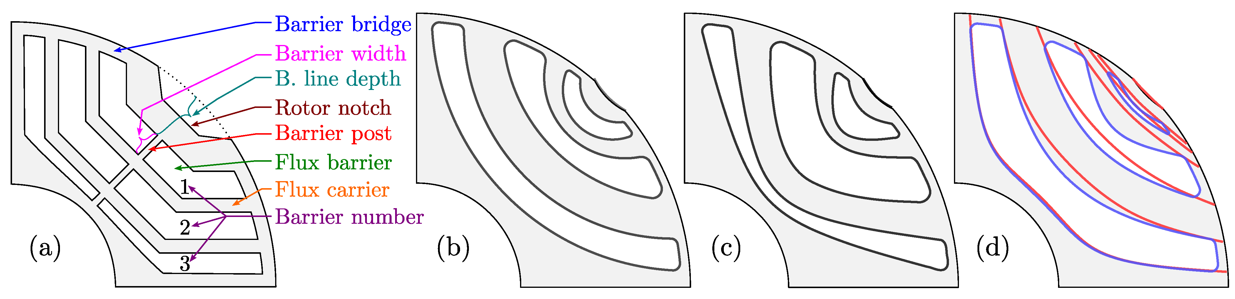
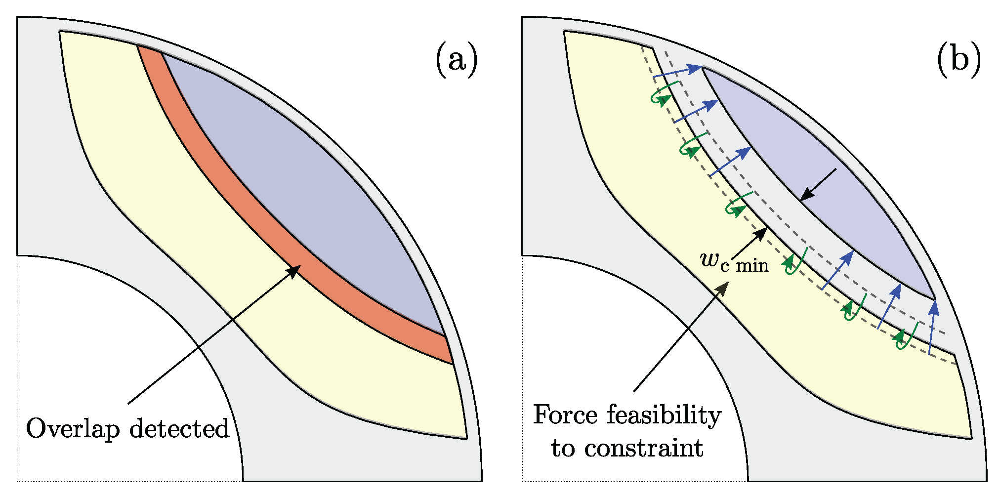
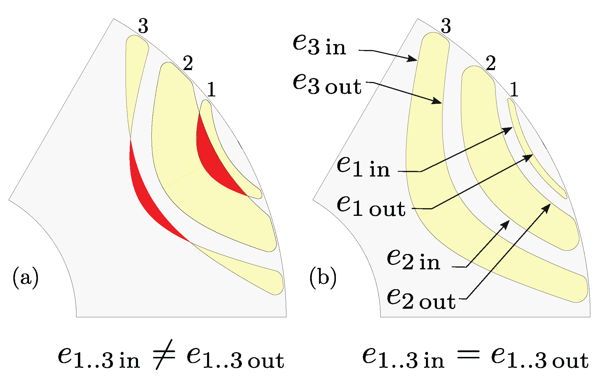
2. Geometric Feasibility
3. Design Automation
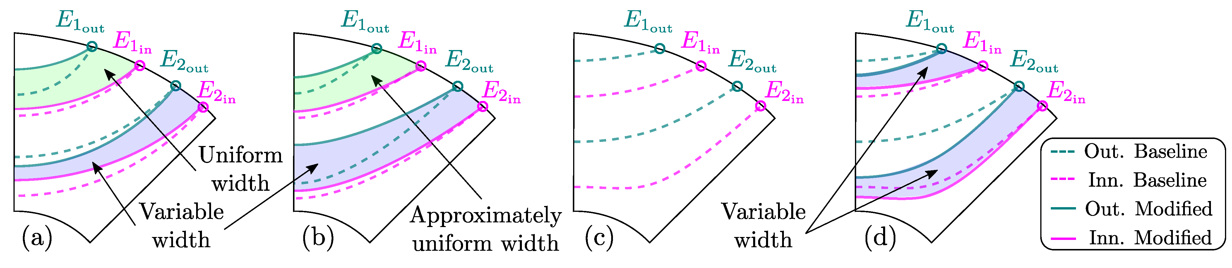
Barrier Depth Variation
4. Standard Rotor Barriers
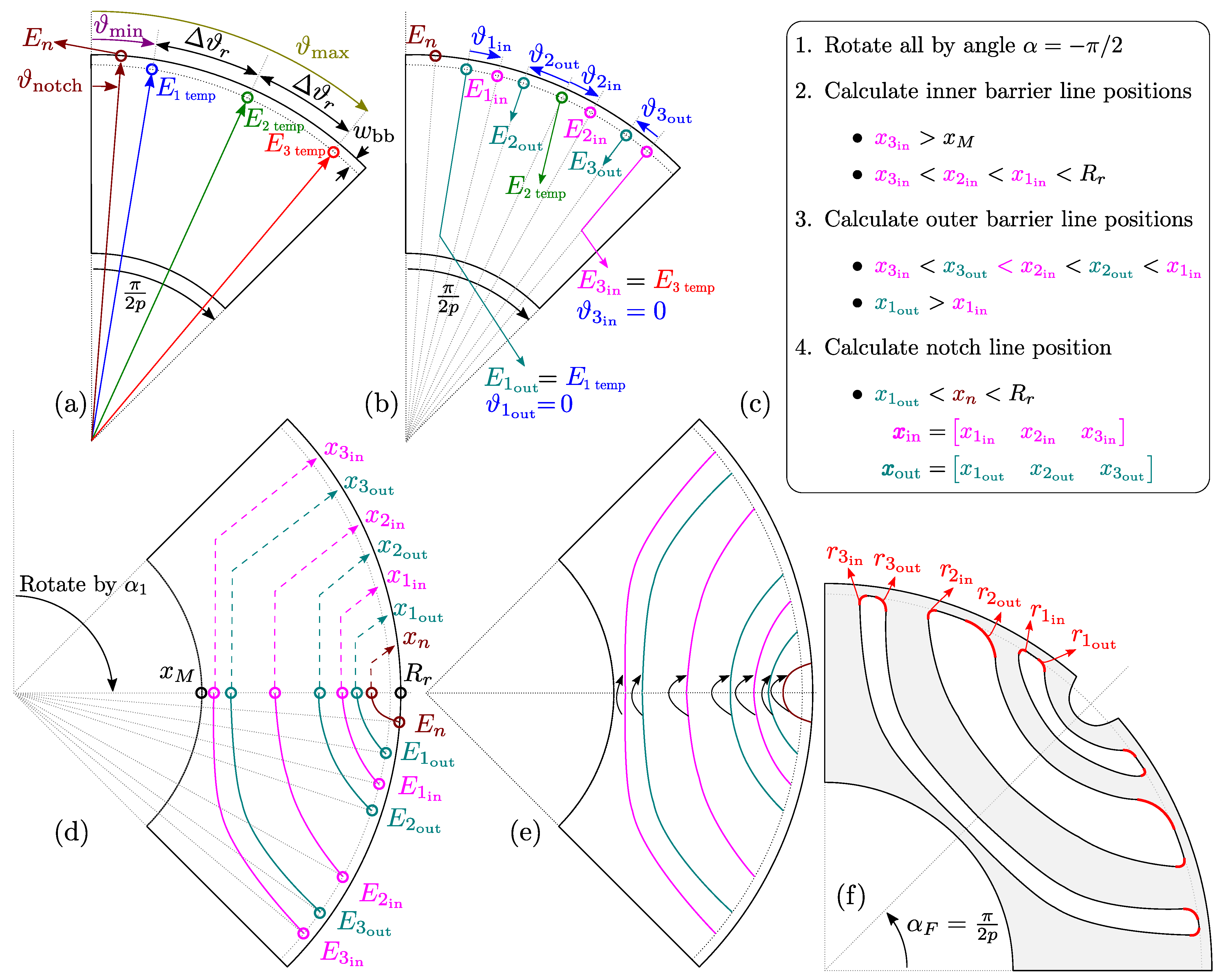
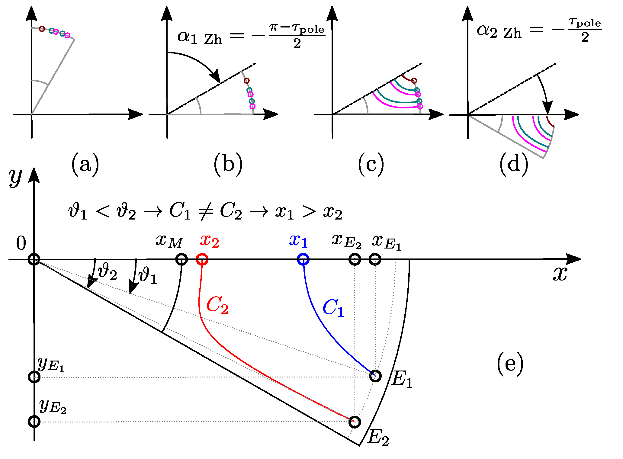
4.1. Zhukovsky Barrier Construction
| Algorithm 1 Construction of Zhukovsky barriers |
|
4.1.1. Inner Line Calculation
4.1.2. Outer Line Calculation
4.1.3. Notch Line Calculation
4.2. Circular Barrier Construction
4.2.1. Inner Line Calculation
4.2.2. Outer Line Calculation
4.2.3. Notch Line Calculation
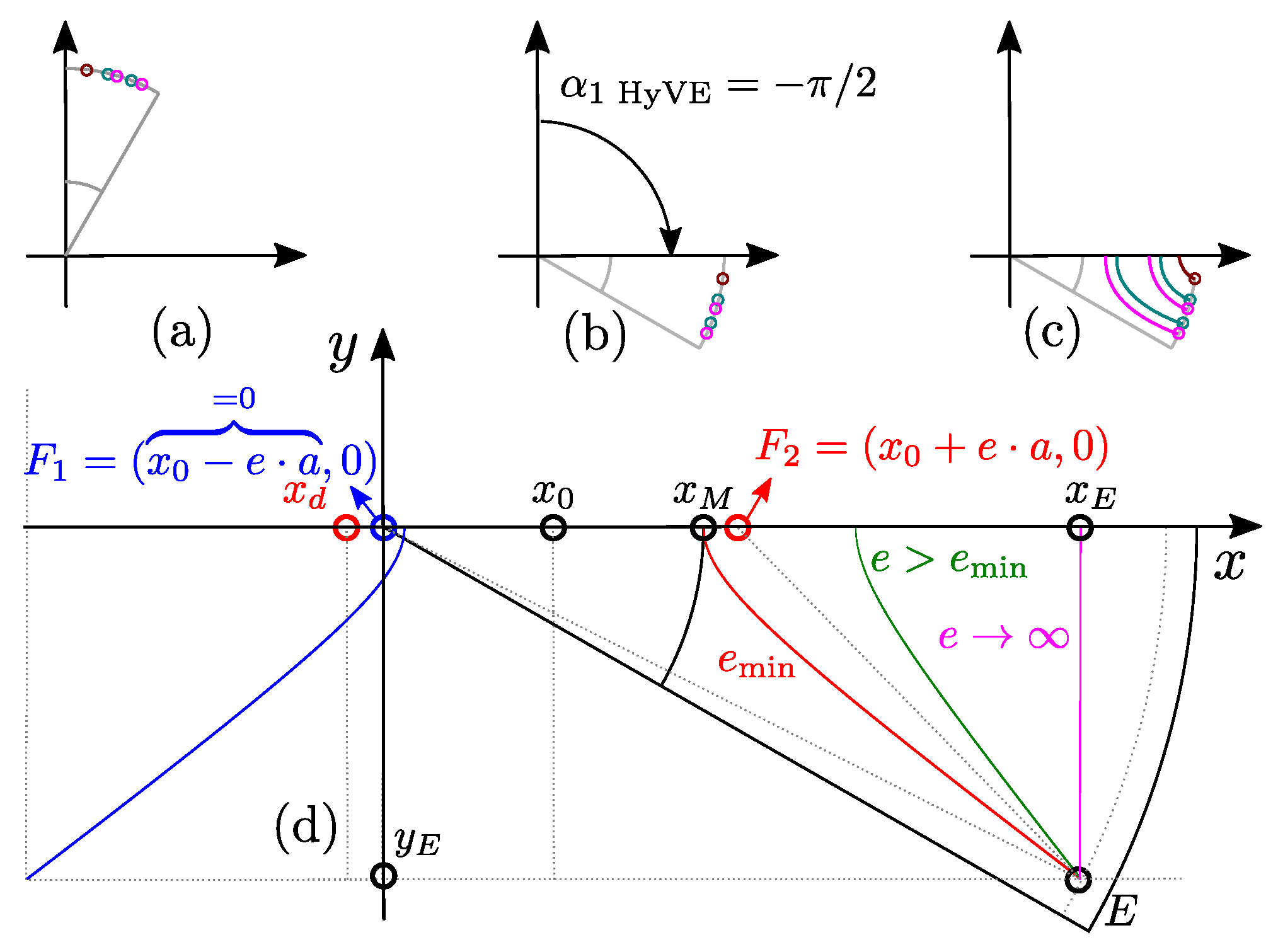
4.3. Hyperbolic Barrier Construction
| Algorithm 2 Construction of circular barriers |
|
| Algorithm 3 Construction of Hyperbolic barriers |
|
4.3.1. Inner Line Calculation
4.3.2. Outer line calculation
4.3.3. Notch line calculation
5. Conformal Modifications
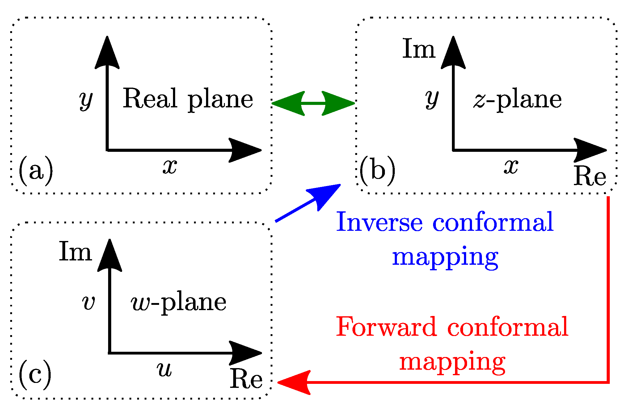
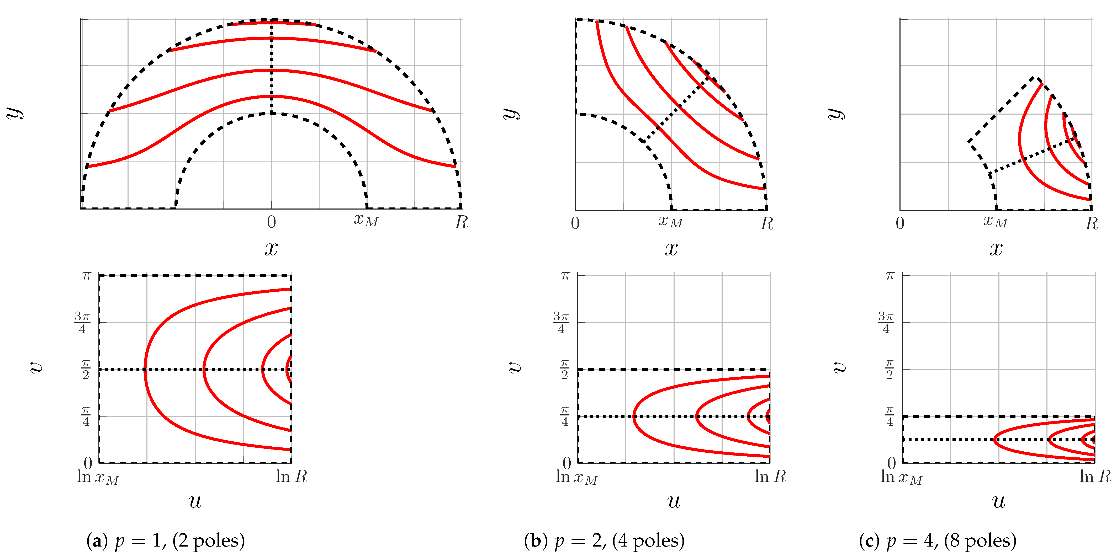
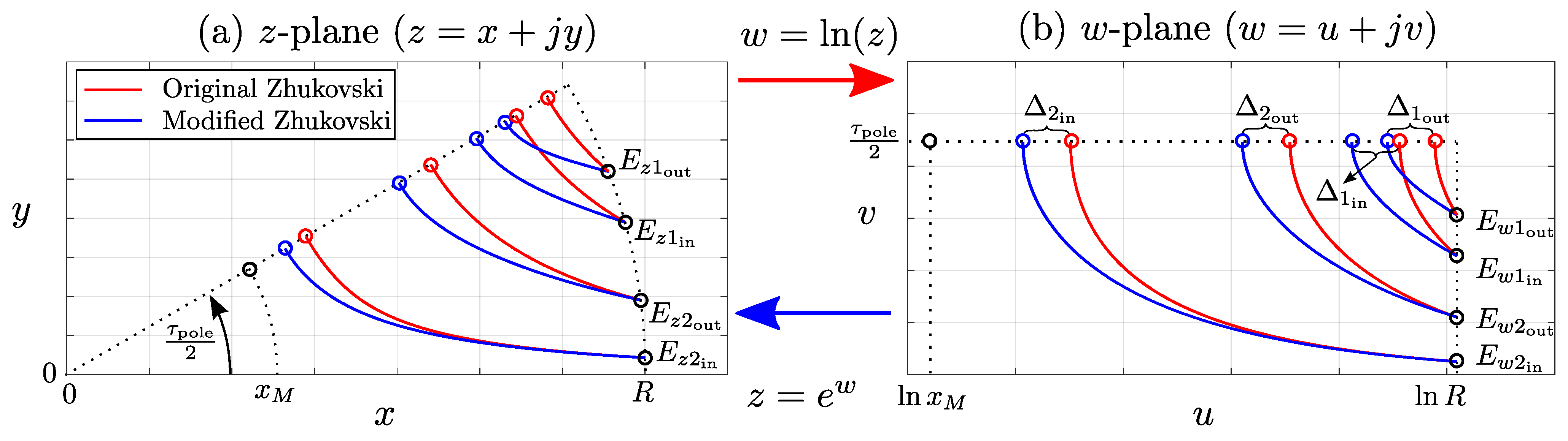
5.1. Conformal Mapping
5.2. Mapping Workflow
5.3. Complex Functions
5.3.1. Forward Conformal Mapping
5.3.2. Inverse Conformal Mapping
5.4. Depth Modification
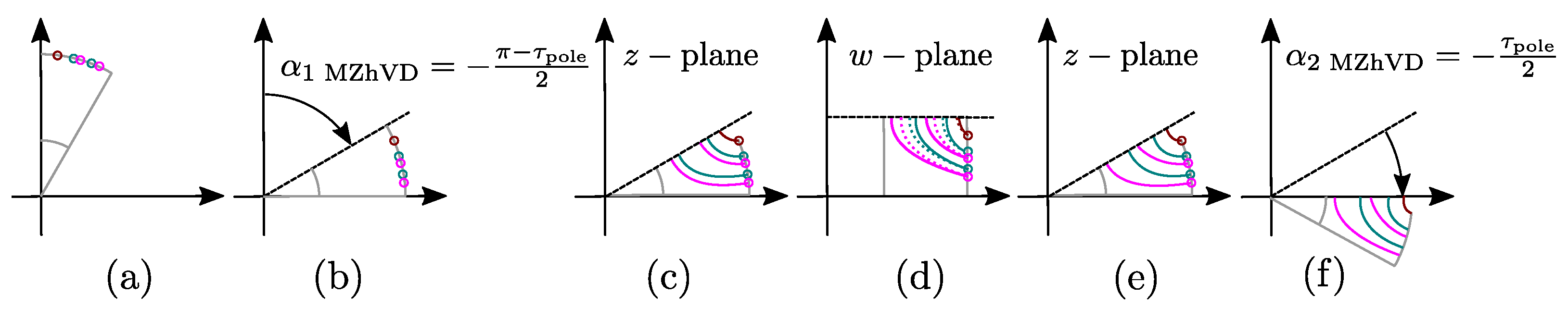
5.5. Modified Zh Barrier Construction
5.5.1. Inner Line Calculation
5.5.2. Outer Line Calculation
5.5.3. Notch Line Calculation
| Algorithm 4 Construction of Modified Zhukovsky barriers |
|
6. Parametric Complexity
7. Pseudo-Code Validation
- Circular concentric (CrC)
- Circular variable depth (CrVD)
- Hyperbolic with fixed eccentricity (HyFE)
- Hyperbolic with variable eccentricity (HyVE)
- Original Zhukovsky (Zh)
- Modified Zhukovsky variable depth (MZhVD)
- Modified Zhukovsky with equal barrier depth (MZhED)
8. Conclusions
Author Contributions
Funding
Institutional Review Board Statement
Informed Consent Statement
Data Availability Statement
Acknowledgments
Conflicts of Interest
Abbreviations
| Abbreviation | Description |
| EV | Electric vehicle |
| FEA | Finite element analysis |
| IPM | Interior permanent magnet |
| IM | Induction machine |
| CrC | Circular concentric barrier |
| CrVD | Circular variable depth barrier |
| HyFE | Hyperbolic fixed eccentricity barrier |
| HyVE | Hyperbolic variable eccentricity barrier |
| Zh | Original Zhukovsky barrier |
| MZhED | Modified Zhukovsky equal depth barrier |
| MZhVD | Modified Zhukovsky variable depth barrier |
| PM | Permanent magnet |
| PTO | Power take off |
| e-PTO | Electric power take off |
| SyRM | Synchronous reluctance machine |
| TPV | Torque per volume |
Appendix A. Variable List

| No. | Variable | Description | No. | Variable | Description |
|---|---|---|---|---|---|
| 1 | Minimum flux carrier width | 33 | First rotation angle in Zh generation | ||
| 2 | Inner barrier depth parameters | 34 | Second rotation angle in Zh generation | ||
| 3 | Outer barrier depth parameters | 35 | First rotation angle in Zh generation | ||
| 4 | Notch depth parameter | 36 | First rotation angle in Zh generation | ||
| 5 | p | Number of pole pairs | 37 | First rotation angle in MZhVD generation | |
| 6 | k | Number of flux barriers | 38 | Second rotation angle in MZhVD generation | |
| 7 | Minimum angular barrier span | 39 | Radial Zhukovsky line coordinate vector | ||
| 8 | Maximum angular barrier span | 40 | Angular Zhukovsky line coordinate vector | ||
| 9 | Angle of one pole | 41 | Zhukovsky line coefficient | ||
| 10 | First rotation angle in example figure | 42 | Line starting point angular coordinates | ||
| 11 | Initial construction points | 43 | Inner line starting point horizontal coordinates | ||
| 12 | Available angular space | 44 | Inner line starting point vertical coordinates | ||
| 13 | Barrier bridge vector | 45 | Circular barrier center coordinate vector | ||
| 14 | Notch line starting point | 46 | Circular barrier radius vector | ||
| 15 | Notch line starting point angular coordinate | 47 | Minimal eccentricity vector | ||
| 16 | Inner barrier line starting point vector | 48 | Line starting point radial coordinate vector | ||
| 17 | Outer barrier line starting point vector | 49 | Line starting point angular coordinate vector | ||
| 18 | Initial barrier construction angular coord. | 50 | Eccentricity vector | ||
| 19 | Inner barrier line starting point radial coord. | 51 | Left directrix of hyperbola | ||
| 20 | Outer barrier line starting point radial coord. | 52 | Horizontal w-plane coordinate vector | ||
| 21 | Inner barrier line starting point angular coord. | 53 | Vertical w-plane coordinate vector | ||
| 22 | Outer barrier line starting point angular coord. | 54 | z-plane Zh horizontal vertex vector | ||
| 23 | Inner barrier line intersection point vector | 55 | z-plane Zh vertical vertex vector | ||
| 24 | Outer barrier line intersection point vector | 56 | w-plane Zh horizontal vertex vector | ||
| 25 | Inner barrier line horizontal vertex vector | 57 | w-plane Zh vertical vertex vector | ||
| 26 | Inner barrier line vertical vertex vector | 58 | w-plane Zh intersections vector | ||
| 27 | Outer barrier line horizontal vertex vector | 59 | w-plane shaft limit | ||
| 28 | Outer barrier line vertical vertex vector | 60 | w-plane MZhVD inner barrier intersections | ||
| 29 | Notch horizontal vertex vector | 61 | w-plane MZhVD outer barrier intersections | ||
| 30 | Notch vertical vertex vector | 62 | Period vector of MZhVD cosine offset | ||
| 31 | Inner barrier fillet vector | 63 | Frequency vector of MZhVD cosine offset | ||
| 32 | Outer barrier fillet vector | 64 | Barrier depth offset maximum vector | ||
| 33 | Final rotation angle | 65 | MZhVD Barrier depth offset vector |
References
- Bourzac, K. The Rare-Earth Crisis. Technol. Rev. 2011, 114, 58–63. [Google Scholar]
- Justin, R. Rare earths: Neither rare, nor earths. BBC News, 23 March 2014. [Google Scholar]
- Hong, H.S.; Liu, H.C.; Cho, S.Y.; Lee, J.; Jin, C.S. Design of High-End Synchronous Reluctance Motor Using 3-D Printing Technology. IEEE Trans. Magn. 2017, 53, 4–8. [Google Scholar] [CrossRef]
- Yamashita, Y.; Okamoto, Y. Design Optimization of Synchronous Reluctance Motor for Reducing Iron Loss and Improving Torque Characteristics Using Topology Optimization Based on the Level-Set Method. IEEE Trans. Magn. 2020, 56, 36–39. [Google Scholar] [CrossRef]
- Ban, B.; Stipetić, S. Electric Multipurpose Vehicle Power Take-Off: Overview, Load Cycles and Actuation via Synchronous Reluctance Machine. In Proceedings of the 2019 International Aegean Conference on Electrical Machines and Power Electronics (ACEMP) & 2019 International Conference on Optimization of Electrical and Electronic Equipment (OPTIM), Istanbul, Turkey, 27–29 August 2019. [Google Scholar]
- Ban, B.; Stipetic, S. Design and optimization of synchronous reluctance machine for actuation of electric multi-purpose vehicle power take-off. In Proceedings of the 2020 International Conference on Electrical Machines (ICEM), Göteborg, Sweden, 23–26 August 2020; pp. 1750–1757. [Google Scholar]
- Ban, B.; Stipetic, S.; Jercic, T. Minimum set of rotor parameters for synchronous reluctance machine and improved optimization convergence via forced rotor barrier feasibility. Energies 2021, 14, 2744. [Google Scholar] [CrossRef]
- Hubert, T.; Reinlein, M.; Kremser, A.; Herzog, H.G. Torque ripple minimization of reluctance synchronous machines by continuous and discrete rotor skewing. In Proceedings of the 2015 5th International Electric Drives Production Conference (EDPC), Nürnberg, Germany, 15–16 September 2015. [Google Scholar]
- Ferrari, S. Design, Analysis and Testing Procedures for Synchronous Reluctance and Permanent Magnet Machines. Doctoral Thesis, Politecnico di Torino, Torino, Italy, 2020. [Google Scholar]
- Stipetic, S.; Zarko, D.; Cavar, N. Design Methodology for Series of IE4/IE5 Synchronous Reluctance Motors Based on Radial Scaling. In Proceedings of the 2018 23rd International Conference on Electrical Machines (ICEM), Alexandroupoli, Greece, 3–6 September 2018; pp. 146–151. [Google Scholar]
- Mirazimi, M.S.; Kiyoumarsi, A. Magnetic Field Analysis of Multi-Flux-Barrier Interior Permanent-Magnet Motors Through Conformal Mapping. IEEE Trans. Magn. 2017, 53, 7002512. [Google Scholar] [CrossRef]
- Mirazimi, M.S.; Kiyoumarsi, A. Magnetic Field Analysis of SynRel and PMASynRel Machines with Hyperbolic Flux Barriers Using Conformal Mapping. IEEE Trans. Transp. Electrif. 2020, 6, 52–61. [Google Scholar] [CrossRef]
- Taghavi, S.; Pillay, P. Design aspects of a 50hp 6-pole synchronous reluctance motor for electrified powertrain applications. In Proceedings of the IECON 2017—43rd Annual Conference of the IEEE Industrial Electronics Society, Beijing, China, 29 October–1 November 2017; pp. 2252–2257. [Google Scholar]
- Gamba, M.; Pellegrino, G.; Cupertino, F. Optimal number of rotor parameters for the automatic design of Synchronous Reluctance machines. In Proceedings of the 2014 International Conference on Electrical Machines (ICEM 2014), Berlin, Germany, 2–5 September 2014; pp. 1334–1340. [Google Scholar]
- Cupertino, F.; Pellegrino, G.; Cagnetta, P.; Ferrari, S.; Perta, M. SyRE: Synchronous Reluctance (Machines)—Evolution. Available online: https://sourceforge.net/projects/syr-e/ (accessed on 11 March 2021).
- Zarko, D. A Systematic Approach To Optimized Design of Permanent Magnet Motors with Reduced Torque Pulsations. Ph.D. Thesis, University Of Wisconsin-Madison, Madison, WI, USA, 2004. [Google Scholar]
- Weisstein, E.W. Conformal Mapping. Available online: https://mathworld.wolfram.com/ConformalMapping.html (accessed on 11 March 2021).
- Olver, P.J. Complex Analysis and Conformal Mapping, Chapter 6. In Complex Analysis and Conformal Mapping; University of Minnesota: Minneapolis, MN, USA, 2011. [Google Scholar]
- Pellegrino, G.; Cupertino, F.; Gerada, C. Automatic Design of Synchronous Reluctance Motors Focusing on Barrier Shape Optimization. IEEE Trans. Ind. Appl. 2015, 51, 1465–1474. [Google Scholar] [CrossRef]
- Lu, C.; Ferrari, S.; Pellegrino, G. Two Design Procedures for PM Synchronous Machines for Electric Powertrains. IEEE Trans. Transp. Electrif. 2017, 3, 98–107. [Google Scholar] [CrossRef] [Green Version]
- Ban, B.; Stipetić, S. Systematic Metamodel-based Optimization Study of Synchronous Reluctance Machine Rotor Barrier Topologies. Struct. Multidiscipl. Optim. 2022. in review. [Google Scholar]


| No: | Description | Symbol | Value/Range | Unit |
|---|---|---|---|---|
| 1 | Rotor diameter | 100 | mm | |
| 2 | Shaft diameter | 54 | mm | |
| 3 | Barrier number | k | 3 | - |
| 4 | Pole pairs | p | 2 | - |
| 5 | Barrier bridge | 0.3 | mm | |
| 6 | Point angle in | - | ||
| 7 | Point angle out | 0 | - | |
| 8 | Point angle in | - | ||
| 9 | Point angle out | - | ||
| 10 | Point angle in | 0 | - | |
| 11 | Point angle out | - | ||
| 12–14 | Corner rad. in | - | ||
| 15–17 | Corner rad. out | - | ||
| 18 | Min. angle | - | ||
| 19 | Max. angle | - | ||
| 20 | Notch angle | - | ||
| 22–24 | Barrier depths in | - | ||
| 25–27 | Barrier depths out | - | ||
| 28 | Notch depth | - |
| Baseline Barrier Depths | Modified Barrier Depths | ||||||||
|---|---|---|---|---|---|---|---|---|---|
| Abbr. | |||||||||
| (a) | CrVD | 0.35 | 0.50 | 0.65 | 0.90 | 0.40 | 0.55 | 0.70 | 0.80 |
| (b) | HyVE | 0.40 | 0.50 | 0.80 | 0.90 | 0.35 | 0.45 | 0.60 | 0.85 |
| (c) | Zh | 0.10 | 0.45 | 0.60 | 0.85 | - | - | - | - |
| (d) | MZhVD | 0.10 | 0.45 | 0.60 | 0.85 | 0.20 | 0.40 | 0.80 | 0.90 |
| Sum: | Description | Symbol | Topology |
|---|---|---|---|
| 1 | Min. angle | ||
| 2 | Max. angle | ||
| Barrier angle in | |||
| Barrier angle out | |||
| Remove constants | |||
| - | - | Zh | |
| Barrier depths | HyVE | ||
| Barrier depths | CrVD | ||
| MZhVD |
| Topology | Complexity | k = 2 | k = 3 | k = 4 |
|---|---|---|---|---|
| Zhukovsky; Gamba et al. [14] | 6 | 9 | 12 | |
| Circular; Stipetic et al. [10] | 8 | 12 | 16 | |
| Zhukovsky; Ban et al. [7] | 5 | 7 | 9 | |
| Zh | 4 | 6 | 8 | |
| HyVE | 8 | 12 | 16 | |
| CrVD | ||||
| MZhVD |
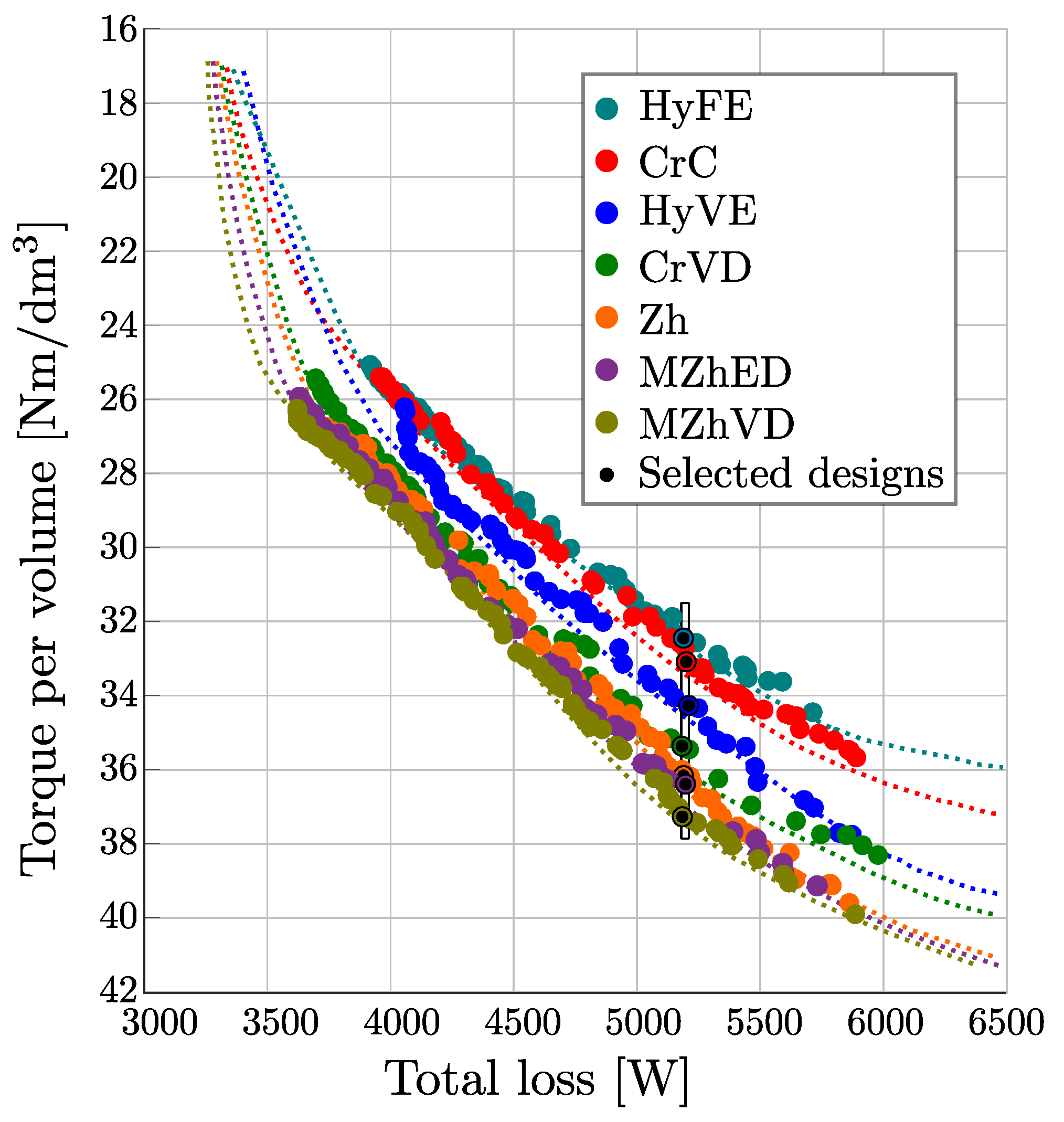
| Name | Unit | HyFE | CrC | HyVE | CrVD | Zh | MZhED | MZhVD |
|---|---|---|---|---|---|---|---|---|
| TPV | Nm/dm3 | 32.5 | 33.1 | 34.3 | 35.4 | 36.2 | 36.4 | 37.3 |
| dm3 | 6.47 | 6.47 | 6.47 | 6.47 | 6.47 | 6.47 | 6.47 | |
| kW | 5188 | 5199 | 5209 | 5182 | 5188 | 5197 | 5184 | |
| kW | 37.4 | 38.1 | 39.5 | 40.8 | 41.7 | 41.9 | 43.0 | |
| Nm | 210.1 | 214.2 | 221.9 | 229.0 | 234.1 | 235.6 | 241.3 | |
| % | 12.1 | 14.1 | 11.7 | 12.7 | 9.7 | 9.3 | 13.7 | |
| n | rpm | 1700 | 1700 | 1700 | 1700 | 1700 | 1700 | 1700 |
| mm | 180 | 180 | 180 | 180 | 180 | 180 | 180 | |
| ∘ | 57.9 | 60.3 | 61.4 | 62.5 | 61.8 | 61.8 | 62.9 | |
| Arms | 95.6 | 95.6 | 94.3 | 94.1 | 95.9 | 95.7 | 95.7 | |
| - | 0.61 | 0.62 | 0.66 | 0.67 | 0.67 | 0.67 | 0.69 | |
| Gain | % | 0.0 | 1.9 | 5.6 | 9.0 | 11.4 | 12.1 | 14.9 |
Publisher’s Note: MDPI stays neutral with regard to jurisdictional claims in published maps and institutional affiliations. |
© 2022 by the authors. Licensee MDPI, Basel, Switzerland. This article is an open access article distributed under the terms and conditions of the Creative Commons Attribution (CC BY) license (https://creativecommons.org/licenses/by/4.0/).
Share and Cite
Ban, B.; Stipetic, S. Absolutely Feasible Synchronous Reluctance Machine Rotor Barrier Topologies with Minimal Parametric Complexity. Machines 2022, 10, 206. https://doi.org/10.3390/machines10030206
Ban B, Stipetic S. Absolutely Feasible Synchronous Reluctance Machine Rotor Barrier Topologies with Minimal Parametric Complexity. Machines. 2022; 10(3):206. https://doi.org/10.3390/machines10030206
Chicago/Turabian StyleBan, Branko, and Stjepan Stipetic. 2022. "Absolutely Feasible Synchronous Reluctance Machine Rotor Barrier Topologies with Minimal Parametric Complexity" Machines 10, no. 3: 206. https://doi.org/10.3390/machines10030206