Article

Online Obstacle Trajectory Prediction for Autonomous Buses

by
Yue Linn Chong
1,†,
Christina Dao Wen Lee
1,*,†,
Liushifeng Chen
1,
Chongjiang Shen
1,
Ken Kok Hoe Chan
2 and
Marcelo H. Ang, Jr.
1
1
Department of Mechanical Engineering, National University of Singapore (NUS), Singapore 119077, Singapore
2
ST Engineering Autonomous Solutions, Singapore 609602, Singapore
*
Author to whom correspondence should be addressed.
These authors contributed equally to this work.
Machines 2022, 10(3), 202; https://doi.org/10.3390/machines10030202
Submission received: 15 February 2022 / Revised: 4 March 2022 / Accepted: 8 March 2022 / Published: 11 March 2022

Abstract

:
We tackle the problem of achieving real-world autonomous driving for buses, where the task is to perceive nearby obstacles and predict their motion in the time ahead, given current and past information of the object. In this paper, we present the development of a modular pipeline for the long-term prediction of dynamic obstacles’ trajectories for an autonomous bus. The pipeline consists of three main tasks, which are the obstacle detection task, tracking task, and trajectory prediction task. Unlike most of the existing literature that performs experiments in the laboratory, our pipeline’s modules are dependent on the introductory modules in the pipeline—it uses the output of previous modules. This best emulates real-world autonomous driving and reflects the errors that may accumulate and cascade from previous modules with less than 100% accuracy. For the trajectory prediction task, we propose a training method to improve the module’s performance and attain a run-time of 10 Hz. We present the practical problems that arise from realising ready-to-deploy autonomous buses and propose methods to overcome these problems for each task. Our Singapore autonomous bus (SGAB) dataset evaluated the pipeline’s performance. The dataset is publicly available online.

1. Introduction

Autonomous driving has become increasingly commonplace around the world. While small vehicles such as cars and mini-buses have seen extensive research and testing, large vehicles such as buses have little research despite their importance in transportation. Buses provide accessible and affordable mobility while reducing traffic congestion. In the coming years, connectivity between people will become increasingly vital as countries leverage intelligent solutions to reduce labor requirements for driving these large vehicles. The automation of large buses can improve the safety and reliability of bus services in an industry plagued by fatigue and stress on bus drivers [1,2,3].
However, published advancements in autonomous driving currently focus on smaller vehicles rather than larger vehicles such as buses. In developing this autonomous bus, we find that new challenges arise, previously undiscovered by research focusing on the smaller autonomous vehicles alone. Most notably, buses have a longer reaction time due to their larger size (typically around 12 m). Due to their large size, these buses usually encounter a larger area of blind spots in the surrounding area; hence, more sensors are required to overcome this.
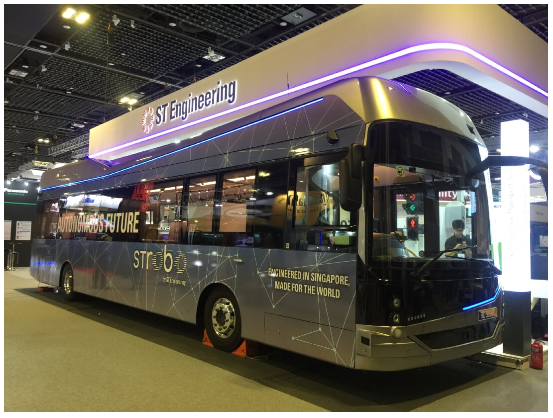
Autonomous vehicle systems plan future motion ahead of time to avoid making sudden manoeuvres. Planning for the future requires the system to predict the future locations of dynamic obstacles to avoid collisions. Smaller autonomous vehicles typically only require planning and prediction up to 5 or 6 s into the future. However, our autonomous buses, one of which is shown in Figure 1, can travel up to 50 km/h and take at least 8 s to react to an obstacle, thereby requiring a longer prediction time horizon. The stopping time is calculated based on the speed limit of buses in Singapore, which is 50 km/h.
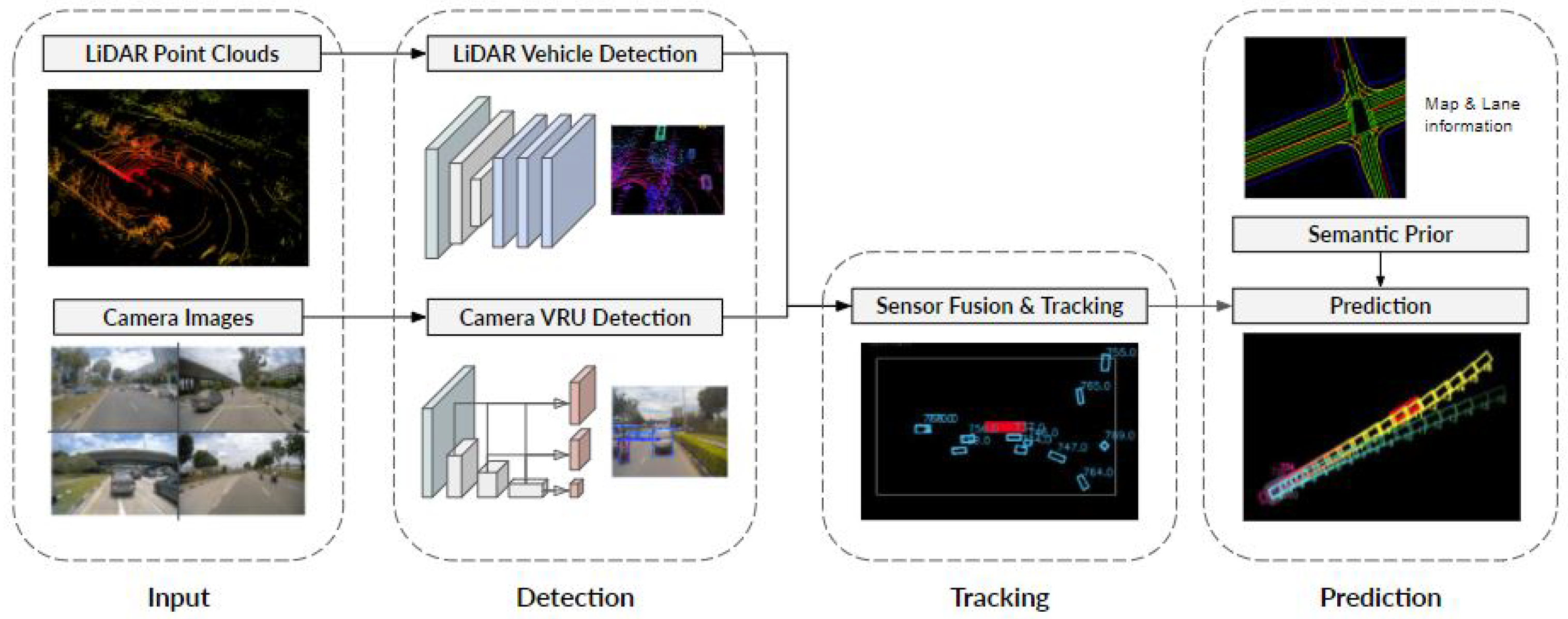
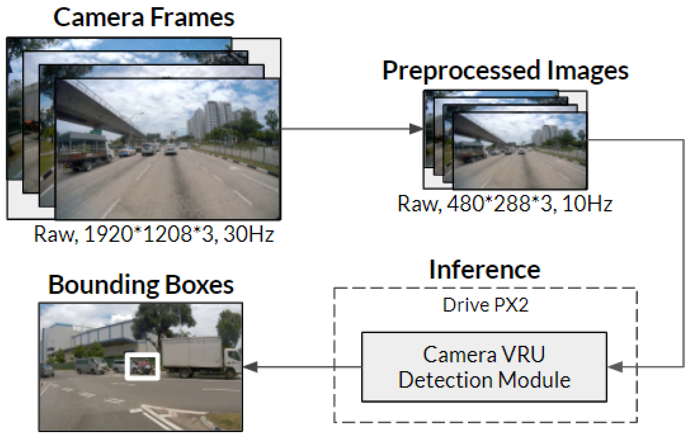
The autonomous bus performs the prediction using a modular prediction pipeline that takes in raw sensor data as input and outputs predicted future states of vehicles and vulnerable road users (VRUs). The perception pipeline is modular, consisting of different perception modules for the following tasks: camera object detection, LiDAR object detection, object tracking and trajectory prediction, as elaborated in Section 4. The pipeline is as follows: raw sensor data are input to the detection modules, the detection modules’ outputs are inputs for the tracker module, and finally, the tracker module outputs are input for the prediction module.
Although this pipeline appears straightforward, its application for the real-world autonomous bus is non-trivial. Specifically, each module’s performance is not perfect. In addition to the highly dynamic environment, there are computational constraints in running the entire pipeline online at a high frequency for reactive planning given the embedded system onboard the autonomous bus. Thus, methods were modified where necessary to achieve the desired computational speed. Due to these constraints, the error of each module may be more significant than that of more accurate but more computationally intensive methods. The erroneous output of the modules is used as input for the subsequent modules, affecting the final trajectory predictions of the prediction pipeline. This paper addresses practical problems that arise from realising ready-to-deploy autonomous buses. We highlight and address the gaps of current methods for each module in the prediction pipeline. Notably, we discuss the practical constraints of limited computing power and how our prediction pipeline balances the trade-off between the inference speed and each module’s performance.
We also introduce the Singapore autonomous bus (SGAB) dataset, which has also been made available publicly on October 2020 at https://arc.nus.edu.sg/project/2020/10/abcd/ and was developed with data collected from our autonomous buses deployed on the public roads of Singapore. Our prediction pipeline was developed and tested on this dataset.
In summary, the contribution of this paper is as follows:
  • We introduce the publicly available dataset for developing autonomous buses, SGAB.
  • For each module in the pipeline shown in Figure 2, we highlight the challenges unique to autonomous buses and propose methods to overcome them.
  • We underscore the effects of the error from the object detection and tracking modules on the performance of the trajectory prediction module and propose a method to reduce the performance degradation due to input error.
The paper is organised in the following manner. Section 2 presents existing work in pipelines for prediction and relevant datasets. Section 3 presents the development of the SGAB dataset. Section 4 gives an overview of the modular prediction pipeline. The LiDAR and camera detection modules are elaborated in Section 5 and Section 6, respectively. Section 7 presents the fusion of the results from the two detection methods and the tracking of dynamic obstacles. Section 8 describes the long-term trajectory prediction module, the effects of erroneous inputs, and a proposed method to minimise error propagation. Finally, we conclude the paper in Section 9.

2. Related Works

Existing literature detailing the development of autonomous buses has been sparse despite the presence of commercial applications [4]. While there have been publications on the motion planning of autonomous buses [5], there is almost no published work that elaborates on obstacle avoidance for autonomous buses. The few papers that cover obstacle avoidance for autonomous buses are either for smaller buses [6] or driving at slow speeds [7] where prediction is not critical since their reaction time is short. In comparison, our 12 m autonomous buses move at speeds up to 50 km/h on public roads with mixed traffic.
For autonomous driving on public roads, prolonged stopping for overly conservative obstacle avoidance is not feasible. Thus, long-term trajectory prediction, i.e., forecasts for longer than one second [8], is necessary, particularly for dynamic obstacles. As publications on long-term trajectory predictions for autonomous buses do not exist to the authors’ knowledge, we instead discuss obstacle trajectory prediction used for autonomous cars. Although the prediction methods included are for generic people trajectory prediction, their approaches are relevant for autonomous buses.
The DARPA Urban Challenge saw the first few modular pipelines for autonomous driving developed. Notably, the Boss entry to this challenge [9] classified tracked obstacles as stationary and moving obstacles; trajectories of moving obstacles were further subdivided into two types: moving obstacles on the road and moving obstacles in unstructured zones such as parking lots. (1) Moving obstacles detected on roads: Their predicted trajectories were under the assumption that they would keep within their lanes. (2) Moving obstacles in free space: Their predicted trajectories used either a bicycle motion model or a constant acceleration motion model using estimated states obtained from tracking. The prediction pipeline of Boss [9] is similar to ours in that the multiple sensor inputs are used for object detection independently and later fused during the association step of tracking. However, there was no analysis of the prediction methods’ performance since the paper focused on implementing the challenge. Moreover, trajectory prediction methods have since improved beyond those used in Boss.
The trajectory prediction methods commonly used can generally be classified into three types: (1) motion model methods, (2) function fitting methods, and (3) deep learning methods. Trajectory prediction for vehicles commonly uses motion model methods [10,11,12,13] as vehicles are nonholonomic platforms that have a fixed range of motion. However, unlike vehicles, pedestrians’ motions tend to be more erratic and difficult to model. The accuracy of the motion model methods heavily relies on how closely the models used can estimate the motion of the target obstacles. Due to the simplicity of the motion models used, most studies predict a shorter time horizon. However, recent work [14] had suggested the possibility that constant velocity motion models may outperform state-of-the-art approaches for longer time horizons. However, the explanation for such results is unique to the datasets where regions of interest are fixed. In contrast, the trajectory prediction for an autonomous vehicle has a moving region of interest following the ego vehicle’s movement. Their paper was also limited to predicting trajectories of people only. Trajectory prediction for the people class is insufficient for applications of the prediction pipeline that must predict trajectories of vehicles and pedestrians. Moreover, Ref. [14] only explored the shorter time horizon of 4.8 s. Thus, this paper explores the relevance of the work presented in [14] for long-term trajectory prediction in Section 8.
Function fitting methods use polynomials [15,16,17] and Chebyshev polynomials [18] for trajectory prediction. The coefficients of the functions could be obtained using neural networks [15,16] or by using Expectation–Maximisation [18]. Similar to motion model methods, function fitting prediction methods are limited by the functions used, and studies for long-term prediction are limited. However, given the low computational resources required for function fitting models, it was meaningful to explore the use of polynomials for long-term trajectory prediction. Section 8 includes the experiments using function fitting methods.
Deep learning methods for trajectory prediction are gaining popularity over the other methods as deep neural networks can model complex trajectories. Many of the newer methods propose the use of Recurrent Neural Network (RNN) architectures, typically the Long Short-Term Memory (LSTM) [19] or Gated Recurrent Unit (GRU) [20], for trajectory prediction. Commonly, the RNNs are arranged to form an autoencoder, also referred to as the encoder–decoder (ED) network, where LSTM or GRU units create an encoder and another set of LSTM or GRU would form the decoder [21,22,23,24]. Existing methods can be categorised into deterministic and probabilistic methods. Deterministic methods predict discrete future trajectories. Conversely, probabilistic methods predict the probability distribution of multiple possible future trajectories. As predicting and using multiple possible future trajectories require significantly higher computational resources, this work only considers deterministic approaches. The ED has shown to be promising in the results in [22], where the ED yielded the best results for deterministic trajectories. To better capture interactions between objects, some methods use a graph-based network to model the interaction between target objects [25,26,27] but these methods require additional memory for the four-dimensional spatiotemporal graphs, which may grow to be significant for applications such as autonomous vehicles, where the region of interest is highly dynamic.
Other methods for interaction modelling include forming a matrix of hidden states [21], performing iterative refinement [22], or using the other objects around the target as inputs [28]. Among these techniques, the last method gives the least impact on computational resources required with the smallest models. However, the implementation in [28] is very limiting as only neighbouring vehicles at fixed locations are considered. Instead, we propose a different method to input the adjacent obstacles using a layer in the semantic map, as elaborated in Section 8.
Currently, many methods evaluate the prediction module performance using ground truth information as inputs—assuming perfect detection and tracking. Using an ideal detector and tracker is problematic as error propagation from each module to the next along the pipeline would affect the performance of the trajectory prediction.
While we present a modular prediction pipeline, others have proposed end-to-end pipelines instead. In the end-to-end approaches, a deep learning model such as FAF [29] or MMF [30] is trained with sensor information as inputs and directly outputs objects detected, tracked trajectories, and trajectory predictions. These networks perform detection, tracking, and prediction in the same model and may implicitly overcome error propagating between the detection, tracking, and prediction. However, end-to-end methods do not have the benefits of modularity, such as ease of interpretation between tasks. They are also difficult to modify or improve, unlike modular pipelines, which can swap out poorly performing modules without affecting other modules. As end-to-end networks are a single deep learning model, they are also prone to adversarial attacks. Hence, this paper presents a prediction pipeline for autonomous driving leveraging the benefits of modularity but a method to overcome the disadvantage of error propagation between modules in the pipeline.
Overall, the existing literature presents a lack of studies on long-term trajectory prediction, with the most common prediction horizon being up to approximately 5 s [14,21,23,24,25,27]. The authors could only find a single paper that conducted long-term prediction up to 8 s into the future [12]. However, their work heavily focused on predicting lane changes, in contrast to this paper’s mixed and dynamic obstacle trajectory prediction of interest. Moreover, there is no study published on the effects of imperfect inputs on the performance of the long-term trajectory predictions, to the authors’ knowledge. Therefore, this paper bridges this gap by analysing the effects of error in trajectory prediction for long time horizons of 8 s for implementation on autonomous buses. The proposed method also aims to reduce the error propagation in the pipeline.
For deep learning methods, datasets are pivotal in training and testing. There are several public datasets collected for autonomous cars, such as the KITTI [31], Argoverse [32], nuScenes [33], and Waymo Open dataset [34]. However, the only other dataset of data collected for autonomous buses is the Electric Bus Dataset by Autonomous Robots Lab [35], but they do not provide ground truth information of objects in the dataset. Hence, the authors developed and released the annotated Singapore autonomous bus (SGAB) dataset [36] publicly and used this dataset to evaluate the methods presented in this paper. Section 3 elaborates further on the details of the SGAB dataset used.

3. Dataset Development

The SGAB dataset was collected from a 12-m bus fitted with 2D LiDAR, 3D LiDAR, cameras, and radars, as shown in Figure 3. The dataset has been made public on October 2020 at https://arc.nus.edu.sg/project/2020/10/abcd/. We compare the dataset with existing datasets in Table 1.
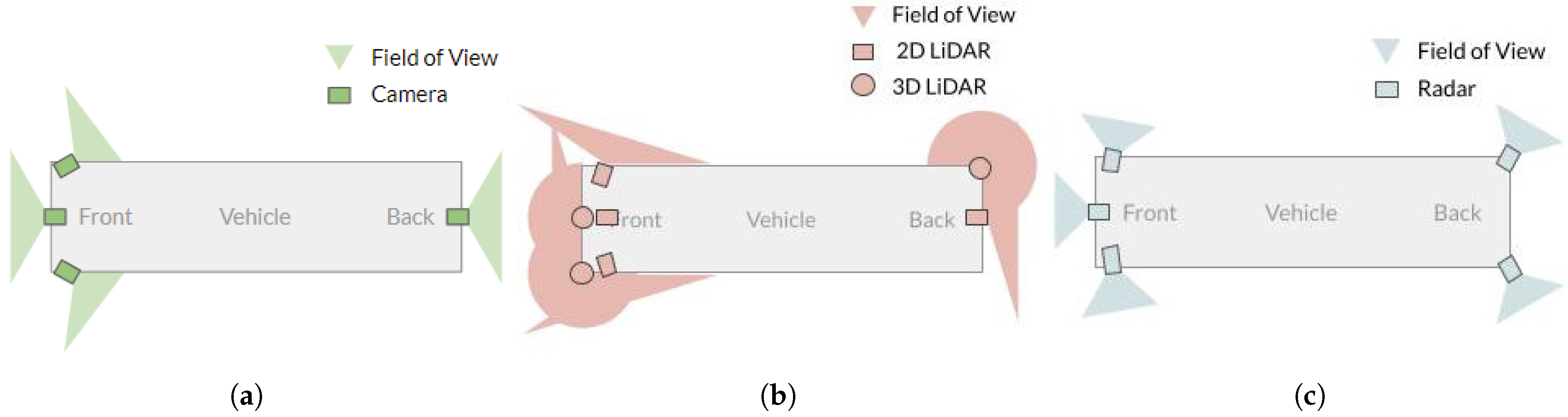
Camera sensors: The location and field of view of the cameras are shown in Figure 3a. There are four 120 field of view cameras on the bus. The side cameras are not placed parallel to the ground.
LiDAR sensors: Seven LiDARs are mounted onto the bus, three 3D LiDARs and four 2D LiDARs. The 3D LiDARs are Velodyne’s VLP-16s (16 layer LiDAR). The 2D LiDARs are Ibeo Scala LiDARs, and we fuse the point cloud data via the Ibeo ECU (a four-layer LiDAR). The LiDARs provide 360 coverage of the environment, as shown in Figure 3b, due to their effective placement on the bus.
Radar sensors: The dataset also includes radar information from five radars mounted as shown in Figure 3c. The radars are Delphi ESR and SRR radars.
The bus has an inertial navigation system (INS) fitted to locate the bus in the world coordinates. We use the Robot Operating System (ROS) middleware [
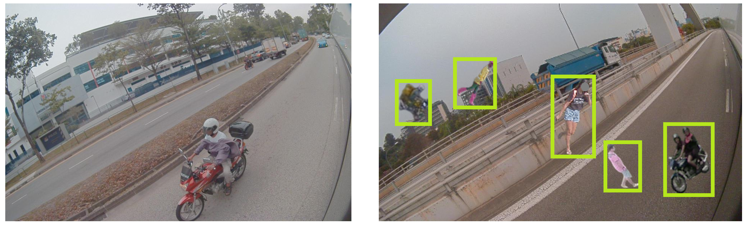
37] to log the sensor data using the rosbag function. We extract the raw sensor at 20 Hz and provide annotations in the LiDAR sensor frame for every ten frames (i.e., at 2 Hz). The annotations are bounding boxes in the LiDAR sensor frame and from the top-down view. We label the objects’ x-position, y-position, width, length, yaw, object class, and ID. Since the annotations are in a top-down view, the height and z-positions are negligible. We label objects within 40 m forward, back, left, and right of the ego vehicle (forms an 80 × 80 m grid). The object classes are: car, truck, bus, pedestrian, bicycle, motorbike, and personal mobility devices (PMD) [36]. A unique ID is given to each tracked object across the sequences.
The data collected were divided into two sets: training and test set. The developed SGAB dataset was then used to test several methods, described in the following sections.

4. Prediction Pipeline Implementation

The prediction pipeline is shown in Figure 2. The input of our prediction pipeline is multi-LiDAR point clouds and multi-camera images. Object detection is done on the LiDAR and camera sensor data separately, and the networks are elaborated in Section 5 and Section 6, respectively. We observed that the radar point cloud was very sparse in the various experiments done. Thus, radar information was not used in the overall pipeline and can be considered for future work. After the detections from both sensor types are fused and concurrently tracked in the top-down view, also known as Bird’s-Eye View (BEV), the task of sensor fusion and tracking is detailed in Section 7. The final prediction module takes in a semantic prior using map and lane information, along with details of tracked objects to perform the multi-object long-term prediction, as explained in Section 8.
Our prediction pipeline was developed and tested on the Nvidia Drive PX2 [38] hardware, and all modules were optimised for real-time computation on this embedded system during autonomous driving. Though the system appears complex, with four modules running on the embedded system, we provide Figure 4 to describe the memory allocation of the different modules on the Nvidia PX2.

5. LiDAR-Based Object Detection

As shown in Figure 3b, the autonomous buses have seven LiDAR sensors. The LiDAR sensors give point cloud data of the scene, which are only used to detect vehicles due to their sparsity. The sparsity is due to the height of the ego vehicle and the few layers of the LiDAR sensors. Hence, this module does not detect obstacles such as pedestrians and cyclists or vulnerable road users (VRUs), which, due to their smaller size, have few points visible in the LiDAR sensor point cloud. Instead, camera sensors are used to detect these smaller obstacles. Detections using camera images are elaborated in Section 6. The detections from the camera and LiDAR data are then fused as discussed in Section 7.
The main challenge faced during the implementation of LiDAR-based detection for online obstacle detection is the inference speed of the module when running on the embedded system of the autonomous buses.
For obstacle avoidance, a high detection rate is required. The 3D LiDARs output sensor data at the rate of 20 Hz. Therefore, detection must be performed under 50 ms when running on the onboard embedded system to use the latest sensor output from these LiDARs. Since the LiDAR sensors are not synchronised, each LiDAR outputs at different timestamps, and for our implementation, only the newest sensor frame of each LiDAR is used. The remainder of this section presents our implementation to speed up LiDAR-based object detection. The deep learning model used is described in Section 5.1 and its performance is presented in Section 5.2.

5.1. LiDAR-Based Object Detection Model

This task is performed using a deep learning network based on PIXOR++ [39], an improved version of the original model [40]. This network is lightweight and has a quick inference time. Note that while the original paper [39] discussed a map estimation network, our work only requires the object detection network.
The PIXOR++ deep learning network takes in a voxelised representation of a single point cloud [39]. As the autonomous bus is a large vehicle with a longer braking distance, seven LiDAR sensors, shown in Figure 3, were used to ensure sufficient coverage of the larger region of interest. Firstly, all LiDAR data were transformed into the coordinate reference frame of the autonomous bus. Of the seven LiDARs, the four Ibeo 2D-LiDARs were then synchronised with the proprietary Ibeo ECU. We combined all the sensor data into a single larger point cloud. This larger point cloud was then concatenated with the most recent point clouds from the three Velodyne 3D-LiDARs. As the number of points in the resultant point cloud is significant, the run-time for pre-processing the point cloud is also significant. However, preliminary experiments on reducing the number of points led to a degradation in performance. Hence, our approach was to parallelise the pre-processing and the inference of the model to achieve the desired output frequency. We also found that the run-time is highly sensitive to the size of the voxels. For the SGAB dataset, we use voxels of size 1.25 m by 1.25 m to achieve the output frequency of 28.5 Hz. The PIXOR++ deep learning network outputs a list of the positions, sizes, and orientations of the detections in BEV in the coordinate reference frame of the autonomous bus.
Building upon [39], we amended the network to run using TensorRT 4, which enables the module to run at a high frequency on the embedded system onboard the autonomous bus. Layers that are not supported by TensorRT are replaced with similar layers. Specifically, the bi-linear up-sampling layer is changed to a 2D convolution transposed layer with kernels that contain values that are learnable. In effect, the up-sampling becomes learnable. The final model runs inference at 28.5 Hz or 35 ms on the Nvidia Drive PX2 embedded system.

5.2. Results and Discussion

For the training of the module, we use the KITTI dataset [31] and perform transfer learning with the SGAB Dataset [36]. The final model was chosen from the best of 50 epochs of the validation set. The performance of the model is calculated as the mean average precision (mAP) [41] at 0.5 intersection over union (IOU). The module records 49.0% mAP, with 88.0% precision and 55.0% recall at the selected confidence threshold on the SGAB test set. The performance of the model is lower than that reported when evaluated using the KITTI Dataset [31], as reported in [39]. The drop in performance is due to the sparser point clouds used as inputs. The region of interest required when evaluating using SGAB is also significantly larger than that of KITTI, which further increases the difficulty of detections in SGAB.

6. Camera-Based Object Detection

Four 120 field-of-view RGB cameras are mounted on the bus, as shown in Figure 3a, to perform camera object detection of VRUs, namely people, cyclists, and motorcyclists, to make up for LiDAR’s poor detection performance on small objects. The pipeline for camera-based object detection is shown in Figure 5. Image streams from these cameras are resized and cropped before being passed to the detection module via ROS. Reduced spatial resolution and frame rate are necessary to reduce internal bandwidth usage without incurring too much computation, which is needed if compression is used. The pre-processed images are then used by the camera-based object detection model, which outputs bounding box detections and a corresponding label of the object type in the image frame.
Similar to the LiDAR-based object detection module, this module must perform inference quickly while maintaining the accuracy of the detections and sharing computational resources with the other modules. This is particularly challenging as the inference must be performed on four camera images simultaneously on the embedded system of the autonomous bus. Moreover, two cameras are mounted on each autonomous bus at an angle such that the field of view is maximised, which brings about novel challenges. Our implementations with methods to overcome challenges are explained in Section 6.1 and their performance is analysed in Section 6.2.

6.1. Camera-Based Object Detection Model

The object detection module for the camera sensor is performed using a Convolutional Neural Network (CNN) model, implemented in Keras with a TensorFlow backend on the Drive PX2 using a ROS wrapper. The YOLOv3-Tiny [42] model is chosen to be the baseline due to its good speed–accuracy trade-off, as evaluated on the MS COCO [43]. Because the model runs faster than our requirement of 10 Hz, we added a convolutional layer and a detection layer to increase its complexity. The extra detection layer allows more detection proposals.
Off-the-shelf camera object detectors are usually trained and evaluated on MS COCO and Pascal VOC 2007 [41], which contain a variety of everyday objects. However, the number of relevant classes is small for our application, with only three classes, namely pedestrians, cyclists, and motorcyclists. However, the algorithm must also detect the objects in all four cameras, positioned differently. The front and back cameras are positioned parallel to the ground plane and located at around eye level. The side cameras are positioned at an angle on top of the bus, therefore presenting a novel viewing angle, as shown in Figure 6. Transfer learning and data augmentation techniques train the algorithm for this particular task.

6.1.1. Data Augmentation

A sufficiently large and diverse dataset is necessary for the successful training of large neural networks. Most public driving datasets record data using cameras mounted upright on top of a sedan or an SUV, unlike our side cameras. Hence, transfer learning with those datasets does not account for the side cameras.
We perform data augmentation on selected side camera images by cropping the VRUs and removing their background using a photo editing tool to overcome this issue. Scale, rotation, mirroring, aspect ratio, brightness, colour variations, and white noise are then introduced to the objects before five of them are randomly chosen to be tiled over a scene. Four thousand such frames are generated from 100 objects and 41 scenes. Since the objects have already been cropped and are tiled programmatically, their bounding box labels can be automatically generated as well.

6.1.2. Transfer Learning

For transfer learning, the first five convolutional layers of DarkNet-19 [44] trained on MS COCO [43] were used to initialise the model since they detect low-level features that are relevant to most natural images. Subsequent layers are randomly initialised.
Frames containing VRUs from MS COCO [43], BDD100K [45], and nuScenes [33] public datasets are selectively extracted. Specifically, we select frames that either contain at least four objects or contain a bicycle and motorbike to balance out the class numbers. The frames were then shuffled with the augmented data to form the training dataset. Shuffling prevents over-fitting to any specific dataset, as individual datasets have their unique characteristics in terms of object appearances that vary across camera setup and collection location. The model is trained over 80,000 iterations, each mini-batch consisting of 16 images and batch size 64, on the composite training dataset.

6.2. Results and Discussion

Table 2 reports the performance of the models on an evaluation dataset that consists of 199 hand-labelled real road data from the SGAB dataset. Our model, YOLOv3-M, has a smaller CNN backbone but the same number of detection layers as YOLOv3. The table records our model’s performance tested with transfer learning, denoted as YOLOv3-M + TL, and with transfer learning and data augmentation, denoted as YOLOv3-M + TL + DA.
The original YOLOv3 [42] trained on the MS COCO dataset [43], which contains the same classes of object VRUs in our dataset, was also included in the table for comparison. The frame rate of each model was calculated using the Tensorflow implementation on the Nvidia Drive PX2 for inference on four camera images simultaneously. From Table 2, the performance on the full-sized YOLOv3 is too slow to meet our high output frequency requirement. In [42], YOLOv3 reported a low inference time of 22 ms on the M40 or Titan X GPUs. However, YOLOv3 on the Nvidia Drive PX2 embedded system has a four-fold increase in inference time. This is attributed to the restricted computing resources that are available on the embedded system despite having multiple hardware accelerators onboard. Therefore, we propose the YOLOv3-M model, which can meet the desired requirement of an output frequency of 10 Hz.
The performance of the YOLOv3 model trained on the MS COCO dataset suffers a performance loss from 28.2% mAP [42] to 16.66% mAP when tested on the SGAB dataset. The drop in performance is due to the shift in the domain between datasets, as elaborated in Section 6.1.1.
We overcome the difference between the datasets with transfer learning using our composite dataset in YOLOv3-M + TL. As a result, we see a significant gain in mAP for our YOLOv3-M model while meeting the desired output frequency of 10 Hz. Adding data augmentation to the training data as described in Section 6.1.1 further improves the model performance significantly. While implementing data augmentation increases the training time, this method does not affect the model size and the output rate. Thus, the proposed method would be to use the YOLOv3-M model with transfer learning and data augmentation.

7. Fusion and Tracking

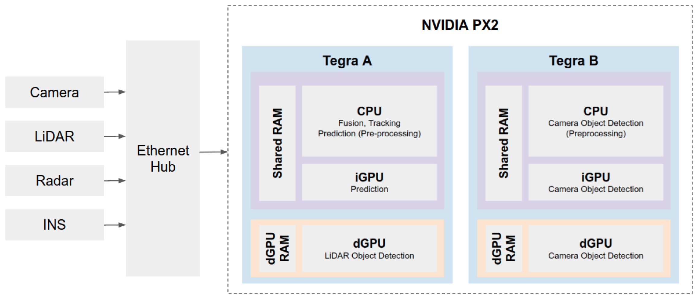
We perform sensor fusion to integrate information from the two sensor types onboard each autonomous bus: LiDARs and cameras. We adopt the late-fusion approach to integrate the LiDAR-based and camera-based detections while simultaneously performing multi-object tracking (MOT) in BEV. Firstly, we select the late fusion method to make full use of the limited GPUs available on the Nvidia PX2 and divide the detection models into two GPUs to improve memory usage. Secondly, the VLP-16 LiDAR’s sparsity made it challenging to perform LiDAR only detection for smaller objects such as pedestrians. It was also computationally expensive to perform feature fusion before detection—for example, generating a depth camera image and fusing it with the raw LiDAR data. Hence, a late fusion method was chosen.
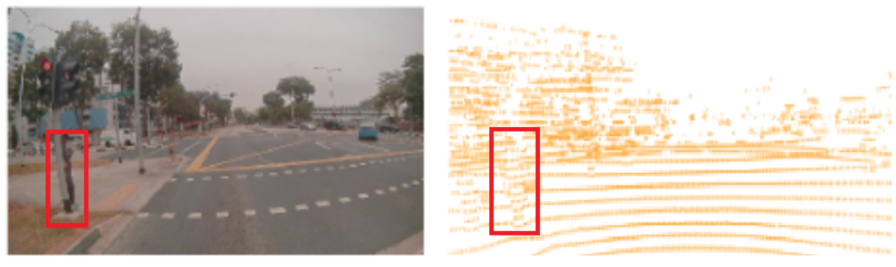
The initial inputs from the detector modules are the camera bounding box detections in the image plane and the LiDAR bounding box detection in BEV. We project the camera bounding boxes into BEV in two steps at this stage. First, we transform the LiDAR point clouds to the image coordinate reference frame as shown in Figure 7. Then, we select the depth value with the highest frequency amongst all points within an object’s 2D bounding box.

7.1. Fusion and Tracking Method

Inspired by AB3DMOT [46], we implemented Kalman filter-based tracking for the multi-object detection state estimation. All detected objects are birthed after being observed for a minimum number of frames and removed after being unseen for a maximum number of frames. During each time step, the module uses a constant velocity (CV) motion model to perform short-term predictions on the states of each object. The predicted states are matched with the detection modules’ outputs. Our method performs sensor fusion from sensor data with different input timestamps. To handle the timestamp differences, we include the time intervals in the CV motion model to give better short-term prediction estimations.
We match the predicted states with the detection modules’ outputs in the association step. We use the IOU to associate the objects with the target for a deterministic tracker. We notice a drawback of using intersection over union (IOU) as a distance measure between predicted and detected states. Mainly, for objects such as people and bicycles, their sizes in BEV are small. Thus, we use a distance-based (L2-norm) association within a threshold to associate currently tracked objects with their corresponding new detections. Finally, the Kalman Filter is utilised to update an object state with associated detections.
To expand on the original AB3DMOT, which uses detections only from the LiDAR point cloud, we use detections from both the LiDAR and camera. We take the camera and LiDAR sensor detections as input to the 3D Kalman filter. This proposed method is agnostic to the type of sensor used as detections are represented as the state information. We consider 14 states in the motion model: [ x , y , z , y a w , w , h , l , x ˙ , y ˙ , z ˙ , x ¨ , y ¨ , z ¨ , y a w ˙ ] .

7.2. Results and Discussion

We present the network’s performance using a deterministic tracker on the SGAB dataset. We evaluated the module using the following tracking metrics: Average Multi-Object Tracking Accuracy (AMOTA) and Average Multi-Object Tracking Precision (AMOTP) [47]. The AMOTA and AMOTP performance calculate the average MOTA and MOTP across the different classes—car, truck, bus, and VRUs (pedestrian, motorcycle, and cyclist), respectively. We use the following covariance matrix values for the tracker.
In our implementation, we tune the covariance matrix of the Kalman filter based on the initial accuracy of the sensor. Using the training split of the SGAB dataset, we calculate the errors in the position and orientation of the detections and further tune the values of the Kalman filter after.
The original AB3DMOT achieves AMOTA of 37.72% and AMOTP% of 64.78% on the KITTI dataset overall for three classes—car, cyclist, and pedestrian. Our final result is a module that outputs at minimally 20 Hz, with AMOTA of 25.61% and AMOTP of 94.52%. Whilst the performance drops compared to the original AB3DMOT work, we highlight that our version is a more accurate reflection of the real-world environment with more classes—truck, bus, and motorcycles. The AMOTP result is high, showing the considerable percentage overlap between the tracked object and the ground truth object. The poor AMOTA value is due to the low detection values from the camera and LiDAR module. Poor detection values in the sparse LiDAR data are found in the SGAB dataset compared to the KITTI dataset.

8. Long-Term Trajectory Prediction

The trajectory prediction module estimates the future position, x t , y t , and orientation, θ t , of the target obstacle at a given time step, t, where the current time step is t = 0.0 ; the module aims to predict the future trajectory, x t = ( x t , y t , θ t ) , for time steps t = 0.5 , 1.0 , 1.5 , , 8.0 s. The time horizon of 8.0 s was chosen to provide sufficient time for the autonomous buses to brake smoothly when avoiding collisions with dynamic obstacles.
The predicted future trajectories are conditioned on the past trajectories of the target object. The past trajectories are obtained from the tracker module during autonomous driving since ground truth information is unknown. However, the past trajectories tracked by the tracker module, i.e., the tracker trajectories, are imperfect, as discussed in Section 7. The error in the tracker trajectories may negatively affect the prediction performance when used as inputs. The implementation of the prediction module compensates for this error due to the modification and delineation, as shown in Section 8.3.
Similar to the other modules in the pipeline, the computational efficiency of the prediction module is a crucial consideration in module development. The method must be able to run on the Nvidia Drive PX2 system alongside other modules for autonomous driving. Thus, a small deep learning model performs prediction, as described in Section 8.2. The model takes in pre-processed data and its outputs are post-processed as described in Section 8.1, and the results of the model are discussed in Section 8.4.

8.1. Inputs and Outputs

The trajectory prediction module takes in the past trajectories of 3 s from the tracker module detailed in Section 7 to perform predictions. We normalise these input trajectories for the deep learning method by scaling the change in position and orientation between time steps of the past trajectories to fit the range from −1 to 1.
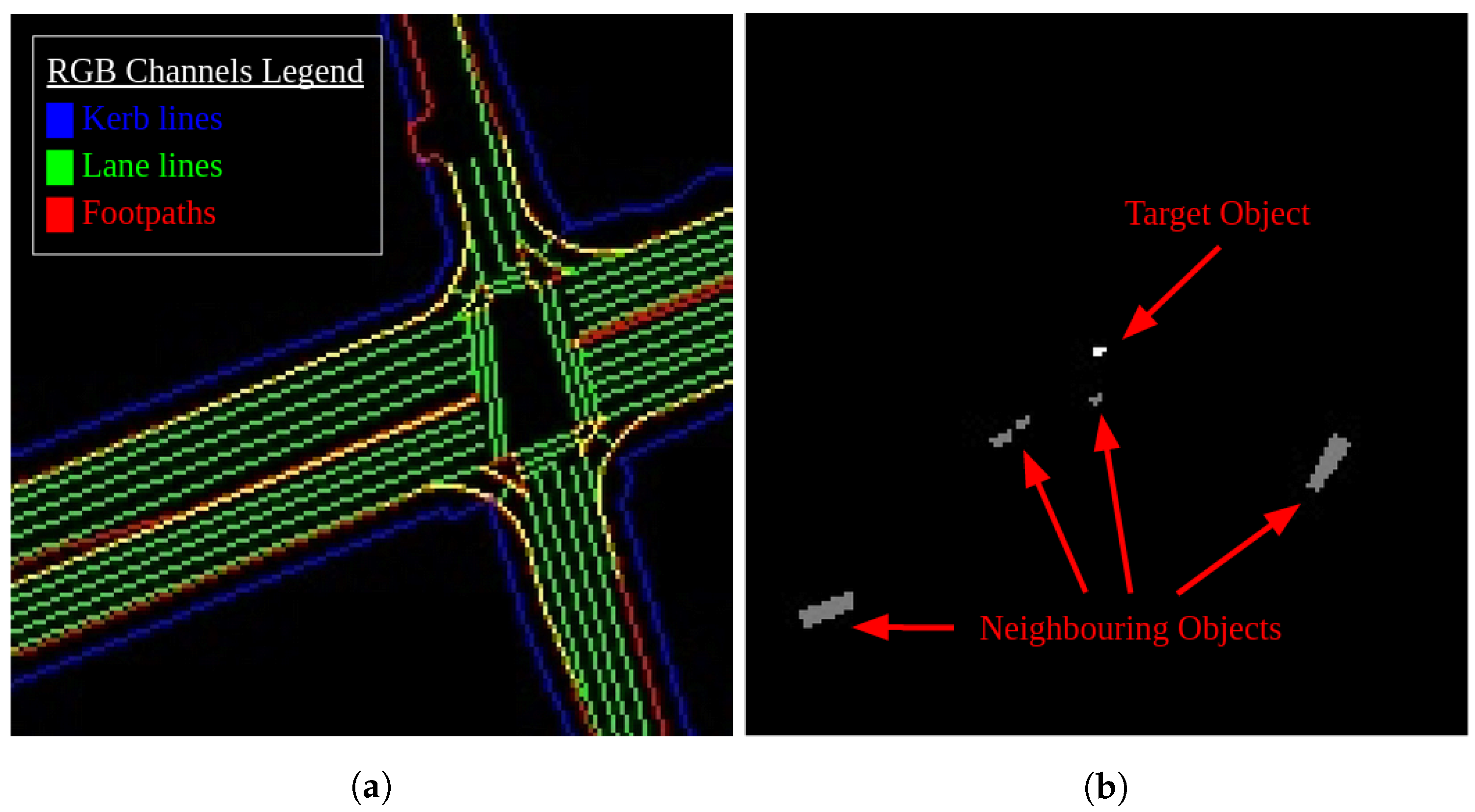
The prediction model also takes in a priori information such as kerbs, lane lines, and footpaths in the form of a semantic map. This information is obtained from the DataMall [48], which is a collection of land transport-related data maintained by the Land and Transport Authority of Singapore. The kerbs, lane lines, and footpaths are drawn with 1 pixel thickness onto separate channels onto an image.
Additionally, the other obstacles in the neighbourhood of the target obstacle are also included in the semantic map to model the interaction between neighbouring obstacles. The resultant semantic map contains four channels, each containing the following semantic information: (i) kerb lines, (ii) lane lines, (iii) footpaths, and (iv) obstacles in the neighbourhood. Figure 8 shows an example of such a semantic map. Each image is centred around the autonomous bus and not the target objects. Instead, the target objects’ location, position, and size are encoded in the semantic map in the obstacles’ channel with a different pixel value. The encoding method reduces the computational requirement for generating new semantic maps for each target object in the scene. For the implementation in ROS, the semantic maps with the kerb lines, lane lines, and footpaths were generated offline and stored as a tiff file such that the global positioning of each pixel is accounted for. During the run, the relevant pixels are read from the tiff file, and the obstacle channel is added based on the outputs of the fusion and tracking module.
The prediction model outputs the scaled change in position and heading of the target object. The predicted future trajectories in the world frame are obtained by scaling back and adding the current position coordinates to the outputs.

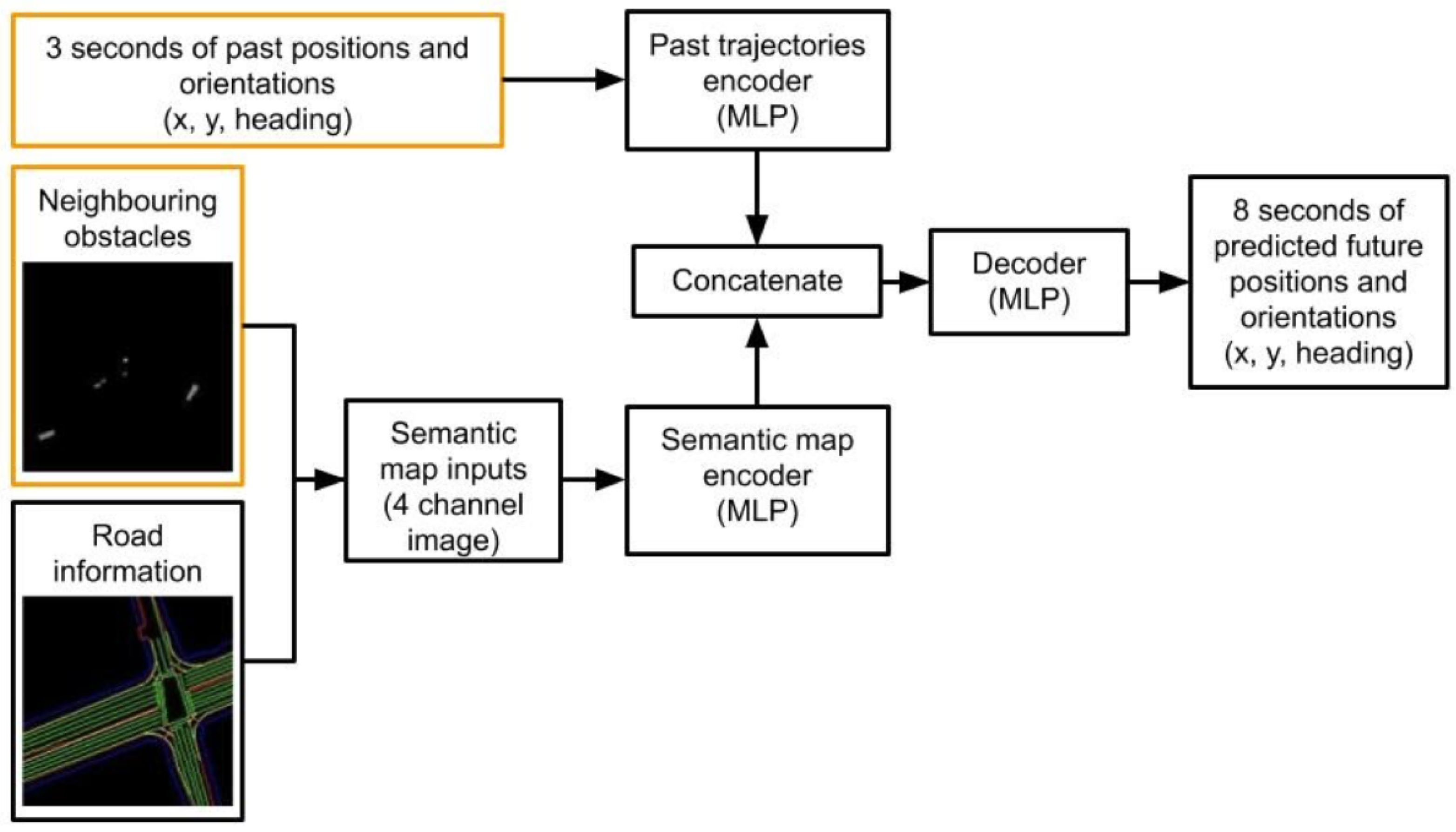
8.2. Model Architecture

Figure 9 shows the architecture of the prediction model. The model is an autoencoder (AE), with an encoder for past trajectories and semantic maps. Features extracted from these encoders are concatenated and passed to the decoder, producing the predicted future trajectories. This paper implements the encoders and decoders using Multi-Layer Perceptrons (MLPs) due to their simplicity and inference speed compared to RNN architectures.
We flatten the semantic map inputs into a one-dimensional array before being fed into the semantic map encoder. The semantic map encoder is an MLP of depth 6 with tanh activation functions, where the number of features in each layer reduces subsequently. Similarly, the past trajectories encoder is an MLP, executed with one hidden layer with a tanh activation function, and the decoder is an MLP with three hidden layers.

8.3. Implementation Details

We train the AE model with past trajectories obtained from the manually annotated ground truths at 2 Hz and the tracker trajectories at 20 Hz. We interpolate the ground truth labels linearly to form the past trajectories at 20 Hz to reconcile the difference in time steps between data points. The semantic map used was 160 by 160 pixels with a resolution of 1 m per pixel. We apply the root mean squared error (RMSE) loss function and the Adam’s optimiser for training in Tensorflow 1.13 with Keras. The weights of the AE model were optimised using the Adam optimiser with a learning rate of 0.001, β 1 of 0.9, and β 2 of 0.999. We ran the training with a batch size of 2 for 100 epochs. The input and output values were normalised by dividing the values by 10.0 m and 100.0 m, respectively. For the positional past trajectories encoder, semantic map encoder, and decoder, 100 hidden units were used in the first hidden layer and progressively reduced along with the depth of the MLP. The tanh activation function was used in all MLPs.

8.4. Experiments, Results, and Discussion

Due to the challenges unique to the autonomous bus, published baselines are not relevant for this section’s scope because they use ideal inputs into a prediction module. The sparser sensor data and larger ROI attributed to the larger size of the autonomous buses result in a more challenging dataset. Thus, several baselines were trained and tested on our dataset, the SGAB dataset [36], to serve as baselines instead. To fully illustrate the impact of the error, we first present experiments on existing methods and their performance, given that the input to the prediction module is ideal. Specifically, we compare the performance of the following prediction methods:
  • Constant position: The future position and orientation of the target object is predicted to remain the same, i.e., the object is assumed to be stationary.
  • Linear fitting: The future trajectories are extrapolated linearly from the past trajectories using least-squares fitting.
  • Quadratic fitting: The future x-positions, y-positions, and orientations are extrapolated from the past trajectories using least-squares fitting onto a quadratic function, respectively.
  • Kalman filter: A Kalman filter with a CV motion model generates the future trajectories by repeatedly using the prediction step. The covariances of the models are hand-tuned on a separate validation set.
  • AE: The future trajectories are obtained using the model described in this paper.
We use the metrics proposed in [21], where the Final Displacement Error (FDE), which is the distance between the ground truth and the prediction at the final time step, and the Average Displacement Error (ADE), which is the average distance between the ground truth and the prediction across time steps, are shown in Table 3.
The high error for the constant position method validates the need for a trajectory prediction module for obstacle avoidance as objects surrounding the vehicle are dynamic in nature and move over a large area over time. The error for the linear fitting method using the SGAB dataset gives the third-highest FDE and ADE error, indicating that the trajectories captured are reasonably non-linear. The method’s performance using the AE model is better than that of the linear fitting method, suggesting that the AE model can better represent the non-linear relationship between the past data with the predicted future trajectories. However, the Kalman filter method achieves a lower FDE and ADE than the AE model and is the best-performing method. The Kalman filter model uses the constant velocity model, which differs from the linear fitting model in that the uncertainty in states is captured as Gaussian noise. Although the Kalman filter method performs better than other methods, the covariances used in the Kalman filter method had to be hand-tuned. While this may have contributed to the better performance, the process was also fairly labour-intensive. Due to this, AE methods are more prevalent in the recent literature. It is also likely that the hand-tuned covariance values used in the Kalman filter are less robust to errors in the input. To study this, we compare the Kalman filter and AE methods when performing prediction with trajectories from Section 7. The variations of the methods implemented with tracker trajectories are as follows:
  • Kalman Filter: The same Kalman filter method used for prediction with labelled ground truth was applied to the tracker trajectories.
  • AE: The tracker outputs were used as input to the same model weights used for prediction with labelled ground truth.
  • AE-T: The AE model architecture described in Section 8.2 was trained on tracker trajectories as past trajectories input with the corresponding ground truth future trajectories.
  • AE-GT: The AE model architecture, described in Section 8.2, was trained on labelled ground truth data. Subsequently, we fine-tuned the network weights using the corresponding tracker trajectories inputs.
  • AE-GT+T (Proposed method): The AE model was trained using the combined data from the labelled ground truth and tracked trajectories.
The evaluation of methods using tracker trajectories differs slightly from the evaluation presented for labelled ground truth input in that incomplete ground truth future trajectories are also used for evaluation. Calculation of the prediction results using tracker trajectories requires the association between the tracker and ground truth labels. However, due to the non-ideal performance of the tracker, the number of tracked objects able to be associated with the labels with complete future ground truth trajectories is too few for evaluation. Table 4 shows the performance of the methods when using tracking trajectories as input.
There is a significant decrease in the performance of the predictions using trajectories from the tracker module compared to using trajectories from ground truth for both the Kalman filter and AE methods. For the Kalman filter method, the error increase from using erroneous inputs is not as significant as that of the AE method. The Kalman filter’s better performance is likely due to good modelling of input uncertainty using Gaussian distributions with zero mean. However, the AE model does not represent input uncertainty, which explains why the error was almost double that of when ground truth annotations were inputs.
In many deep learning applications, improved performance on a different input distribution is achieved by fine-tuning the weights of the model with the new distribution. This was employed in the AE-GT method, but the performance of the model did not improve, suggesting that the erroneous input data were too different from those of the ground truth, and the learning may have reached the local minima instead.
Instead, the AE-T learning to predict the tracker trajectories from scratch yielded significantly improved performance. However, the Kalman filter method still outperformed these methods.
In the AE-GT+T method, we trained the model with ground truth and both types of the tracker to further improve the generalization of the AE model. This process can also be understood as a form of data augmentation, where ground truth data are augmented with imperfect data such that the tracker can predict the correct future trajectory regardless of the input type. Thus, we propose using an AE model trained on both ground truth and tracker inputs with an ADE of 8.24 m.

9. Conclusions

This paper discussed using various sensors onboard an autonomous bus to achieve long-term trajectory prediction online. We presented the practical problems that arise from realising ready-to-deploy autonomous buses. We discussed improving the speed of the LiDAR detection module using modifications to an existing method. We also improved the speed and accuracy of the camera detection module while generalising for camera angles required for autonomous buses. A Kalman filter-based method was also presented for fusing and tracking asynchronous multi-sensor detections. We also proposed a training method where training data are augmented with tracker trajectories to improve the performance of the trajectory prediction model with erroneous inputs. Although the presented long-term trajectory prediction pipeline was for autonomous buses, others could also integrate the pipeline into any other modular autonomous vehicle system. The work presented aims to narrow the gap between research and real-world applications specifically for autonomous driving systems, but the methods proposed could be extended to other real-world pipelines with similar implementations.
Future work can consider using radar data available to perform radar-only or radar-based sensor fusion to improve existing performance for detection, tracking, and prediction. While our modules currently run sufficiently fast for online autonomous driving at 10 Hz, some drop in performance was due to the limited computational resources available on the Nvidia Drive PX2. In future work, we would like to explore more extensive algorithms and more powerful hardware accelerators available.
As we are making the SGAB dataset public, we hope to contribute towards the further development of obstacle trajectory prediction towards realising real-world autonomous bus applications. This would include the exploration of domain adaptation methods to overcome the difference between ground truth and tracker data. We also would like to explore the performance of the proposed methods for autonomous cars via datasets such as the KITTI dataset.

Author Contributions

Conceptualisation and methodology, Y.L.C., C.D.W.L., L.C. and M.H.A.J.; data curation, Y.L.C. and C.D.W.L.; writing—review and editing, Y.L.C. and C.D.W.L.; visualisation, Y.L.C. and C.D.W.L.; supervision, C.S., K.K.H.C. and M.H.A.J. All authors have read and agreed to the published version of the manuscript.

Funding

This research is supported by the National Research Foundation, Prime Minister’s Office, Singapore, under its LTA Urban Mobility Grand Challenge Program, Project Code UM01/002, ST Kinetics autonomous bus trial. Any opinions, findings, and conclusions or recommendations expressed in this material are those of the author(s) and do not reflect the views of the National Research Foundation, Singapore.

Institutional Review Board Statement

Not applicable.

Informed Consent Statement

Not applicable.

Data Availability Statement

Not applicable.

Conflicts of Interest

The authors declare no conflict of interest.

References

  1. Duffy, C.A.; McGoldrick, A.E. Stress and the bus driver in the UK transport industry. Work Stress 1990, 4, 17–27. [Google Scholar] [CrossRef]
  2. Wu, W.T.; Tsai, S.S.; Wang, C.C.; Lin, Y.J.; Wu, T.N.; Shih, T.S.; Liou, S.H. Professional driver’s job stress and 8-year risk of cardiovascular disease: The Taiwan Bus Driver Cohort Study. Epidemiology 2019, 30, S39–S47. [Google Scholar] [CrossRef] [PubMed]
  3. John, L.; Flin, R.; Mearns, K. Bus driver well-being review: 50 years of research. Transp. Res. Part Traffic Psychol. Behav. 2006, 9, 89–114. [Google Scholar]
  4. Azad, M.; Hoseinzadeh, N.; Brakewood, C.; Cherry, C.R.; Han, L.D. Fully Autonomous Buses: A Literature Review and Future Research Directions. J. Adv. Transp. 2019, 2019, 4603548. [Google Scholar] [CrossRef] [Green Version]
  5. Oliveira, R.; Lima, P.; Cirillo, M.; Wahlberg, B. Autonomous Bus Driving: A Novel Motion-Planning Approach. IEEE Veh. Technol. Mag. 2021, 16, 29–37. [Google Scholar] [CrossRef]
  6. Fernández, C.; Domínguez, R.; Fernández-Llorca, D.; Alonso, J.; Sotelo, M.A. Autonomous Navigation and Obstacle Avoidance of a Micro-Bus. Int. J. Adv. Robot. Syst. 2013, 10, 212. [Google Scholar] [CrossRef]
  7. Montes, H.; Salinas, C.; Fernández, R.; Armada, M. An Experimental Platform for Autonomous Bus Development. Appl. Sci. 2017, 7, 1131. [Google Scholar] [CrossRef] [Green Version]
  8. Lefèvre, S.; Vasquez, D.; Laugier, C. A Survey on Motion Prediction and Risk Assessment for Intelligent Vehicles. ROBOMECH J. 2014, 1, 1. [Google Scholar] [CrossRef] [Green Version]
  9. Urmson, C.; Anhalt, J.; Bagnell, D.; Baker, C.; Bittner, R.; Clark, M.N.; Dolan, J.; Duggins, D.; Galatali, T.; Geyer, C.; et al. Autonomous driving in urban environments: Boss and the Urban Challenge. J. Field Robot. 2008, 25, 425–466. [Google Scholar] [CrossRef] [Green Version]
  10. Houenou, A.; Bonnifait, P.; Cherfaoui, V.; Yao, W. Vehicle Trajectory Prediction Based on Motion Model and Maneuver Recognition. In Proceedings of the 2013 IEEE/RSJ International Conference on Intelligent Robots and Systems, Tokyo, Japan, 3–7 November 2013; pp. 4363–4369. [Google Scholar] [CrossRef] [Green Version]
  11. Carvalho, A.; Gao, Y.; Lefevre, S.; Borrelli, F. Stochastic Predictive Control of Autonomous Vehicles in Uncertain Environments. In Proceedings of the 12th International Symposium on Advanced Vehicle Control, Tokyo, Japan, 22–26 September 2014; p. 8. [Google Scholar]
  12. Xie, G.; Gao, H.; Qian, L.; Huang, B.; Li, K.; Wang, J. Vehicle Trajectory Prediction by Integrating Physics- and Maneuver-Based Approaches Using Interactive Multiple Models. IEEE Trans. Ind. Electron. 2017, 65, 5999–6008. [Google Scholar] [CrossRef]
  13. Verma, S.; Eng, Y.H.; Kong, H.X.; Andersen, H.; Meghjani, M.; Leong, W.K.; Shen, X.; Zhang, C.; Ang, M.H.; Rus, D. Vehicle Detection, Tracking and Behavior Analysis in Urban Driving Environments Using Road Context. In Proceedings of the 2018 IEEE International Conference on Robotics and Automation (ICRA), Brisbane, QLD, Australia, 21–25 May 2018; pp. 1413–1420. [Google Scholar] [CrossRef]
  14. Schöller, C.; Aravantinos, V.; Lay, F.; Knoll, A. What the Constant Velocity Model Can Teach Us About Pedestrian Motion Prediction. arXiv 2020, arXiv:1903.07933. [Google Scholar] [CrossRef] [Green Version]
  15. Goldhammer, M.; Köhler, S.; Doll, K.; Sick, B. Camera Based Pedestrian Path Prediction by Means of Polynomial Least-Squares Approximation and Multilayer Perceptron Neural Networks. In Proceedings of the 2015 SAI Intelligent Systems Conference (IntelliSys), London, UK, 10–11 November 2015; pp. 390–399. [Google Scholar] [CrossRef]
  16. Zernetsch, S.; Kohnen, S.; Goldhammer, M.; Doll, K.; Sick, B. Trajectory Prediction of Cyclists Using a Physical Model and an Artificial Neural Network. In Proceedings of the 2016 IEEE Intelligent Vehicles Symposium (IV), Gothenburg, Sweden, 19–22 June 2016; pp. 833–838. [Google Scholar] [CrossRef]
  17. Meghjani, M.; Verma, S.; Eng, Y.H.; Ho, Q.H.; Rus, D.; Ang, M.H. Context-Aware Intention and Trajectory Prediction for Urban Driving Environment. In Proceedings of the 2018 International Symposium on Experimental Robotics, Buenos Aires, Argentina, 5–8 November 2018; Xiao, J., Kröger, T., Khatib, O., Eds.; Springer: Cham, Switzerland, 2018; pp. 339–349. [Google Scholar]
  18. Wiest, J.; Höffken, M.; Kreßel, U.; Dietmayer, K. Probabilistic Trajectory Prediction with Gaussian Mixture Models. In Proceedings of the 2012 IEEE Intelligent Vehicles Symposium, Madrid, Spain, 3–7 June 2012; pp. 141–146. [Google Scholar] [CrossRef]
  19. Hochreiter, S.; Schmidhuber, J. Long Short-Term Memory. Neural Comput. 1997, 9, 1735–1780. [Google Scholar] [CrossRef] [PubMed]
  20. Cho, K.; van Merrienboer, B.; Gulcehre, C.; Bahdanau, D.; Bougares, F.; Schwenk, H.; Bengio, Y. Learning Phrase Representations Using RNN Encoder-Decoder for Statistical Machine Translation. arXiv 2014, arXiv:1406.1078. [Google Scholar]
  21. Alahi, A.; Goel, K.; Ramanathan, V.; Robicquet, A.; Fei-Fei, L.; Savarese, S. Social LSTM: Human Trajectory Prediction in Crowded Spaces. In Proceedings of the 2016 IEEE Conference on Computer Vision and Pattern Recognition (CVPR), Las Vegas, NV, USA, 27–30 June 2016; pp. 961–971. [Google Scholar] [CrossRef] [Green Version]
  22. Lee, N.; Choi, W.; Vernaza, P.; Choy, C.B.; Torr, P.H.S.; Chandraker, M. DESIRE: Distant Future Prediction in Dynamic Scenes with Interacting Agents. In Proceedings of the 2017 IEEE Conference on Computer Vision and Pattern Recognition (CVPR), Honolulu, HI, USA, 21–26 July 2017; pp. 2165–2174. [Google Scholar] [CrossRef] [Green Version]
  23. Chandra, R.; Bhattacharya, U.; Bera, A.; Manocha, D. TraPHic: Trajectory Prediction in Dense and Heterogeneous Traffic Using Weighted Interactions. In Proceedings of the 2019 IEEE/CVF Conference on Computer Vision and Pattern Recognition (CVPR), Long Beach, CA, USA, 15–20 June 2019; pp. 8475–8484. [Google Scholar] [CrossRef] [Green Version]
  24. Gupta, A.; Johnson, J.; Fei-Fei, L.; Savarese, S.; Alahi, A. Social GAN: Socially Acceptable Trajectories with Generative Adversarial Networks. In Proceedings of the 2018 IEEE/CVF Conference on Computer Vision and Pattern Recognition, Salt Lake City, UT, USA, 18–23 June 2018; pp. 2255–2264. [Google Scholar] [CrossRef] [Green Version]
  25. Vemula, A.; Muelling, K.; Oh, J. Social Attention: Modeling Attention in Human Crowds. arXiv 2017, arXiv:1710.04689. [Google Scholar]
  26. Ma, Y.; Zhu, X.; Zhang, S.; Yang, R.; Wang, W.; Manocha, D. TrafficPredict: Trajectory Prediction for Heterogeneous Traffic-Agents. arXiv 2018, arXiv:1811.02146. [Google Scholar] [CrossRef] [Green Version]
  27. Mohamed, A.; Qian, K.; Elhoseiny, M.; Claudel, C. Social-STGCNN: A Social Spatio-Temporal Graph Convolutional Neural Network for Human Trajectory Prediction. In Proceedings of the 2020 IEEE/CVF Conference on Computer Vision and Pattern Recognition (CVPR), Seattle, WA, USA, 13–19 June 2020; pp. 14412–14420. [Google Scholar] [CrossRef]
  28. Altché, F.; Fortelle, A.d.L. An LSTM Network for Highway Trajectory Prediction. In Proceedings of the 2017 IEEE 20th International Conference on Intelligent Transportation Systems (ITSC), Yokohama, Japan, 16–19 October 2017; pp. 353–359. [Google Scholar] [CrossRef] [Green Version]
  29. Luo, W.; Yang, B.; Urtasun, R. Fast and Furious: Real Time End-to-End 3D Detection, Tracking and Motion Forecasting with a Single Convolutional Net. In Proceedings of the 2018 IEEE/CVF Conference on Computer Vision and Pattern Recognition, Salt Lake City, UT, USA, 18–22 June 2018; IEEE: Salt Lake City, UT, USA, 2018; pp. 3569–3577. [Google Scholar] [CrossRef]
  30. Liang, M.; Yang, B.; Chen, Y.; Hu, R.; Urtasun, R. Multi-Task Multi-Sensor Fusion for 3D Object Detection. In Proceedings of the 2019 IEEE/CVF Conference on Computer Vision and Pattern Recognition (CVPR), Long Beach, CA, USA, 15–20 June 2019; IEEE: Long Beach, CA, USA, 2019; pp. 7337–7345. [Google Scholar] [CrossRef]
  31. Geiger, A.; Lenz, P.; Urtasun, R. Are we ready for Autonomous Driving? The KITTI Vision Benchmark Suite. In Proceedings of the Conference on Computer Vision and Pattern Recognition (CVPR), Providence, RI, USA, 16–21 June 2012. [Google Scholar]
  32. Chang, M.F.; Lambert, J.W.; Sangkloy, P.; Singh, J.; Bak, S.; Hartnett, A.; Wang, D.; Carr, P.; Lucey, S.; Ramanan, D.; et al. Argoverse: 3D Tracking and Forecasting with Rich Maps. In Proceedings of the Conference on Computer Vision and Pattern Recognition (CVPR), Long Beach, CA, USA, 16–20 June 2019. [Google Scholar]
  33. Caesar, H.; Bankiti, V.; Lang, A.H.; Vora, S.; Liong, V.E.; Xu, Q.; Krishnan, A.; Pan, Y.; Baldan, G.; Beijbom, O. nuScenes: A multimodal dataset for autonomous driving. arXiv 2019, arXiv:1903.11027. [Google Scholar]
  34. Sun, P.; Kretzschmar, H.; Dotiwalla, X.; Chouard, A.; Patnaik, V.; Tsui, P.; Guo, J.; Zhou, Y.; Chai, Y.; Caine, B.; et al. Scalability in perception for autonomous driving: Waymo open dataset. In Proceedings of the IEEE/CVF Conference on Computer Vision and Pattern Recognition, Virtual, 16–18 June 2020; pp. 2446–2454. [Google Scholar]
  35. Electric Bus Datasets-Autonomous Robots Lab. Available online: https://www.autonomousrobotslab.com/electric-bus-datasets.html (accessed on 15 May 2021).
  36. Chong, Y.L.; Lee, C.D.W.; Chen, L.S.; Shen, C.; Ang, M.H.; Chan, K.K.H. Singapore Autonomous Bus Dataset; National University of Singapore: Singapore, 2020. [Google Scholar]
  37. ROS.Org|Powering the World’s Robots. Available online: https://www.ros.org/ (accessed on 15 May 2021).
  38. NvidiaPX_Linux_DPX_SDK. Available online: https://docs.nvidia.com/drive/active/5.0.10.3L/nvvib_docs/index.html#page/NVIDIA%2520DRIVE%2520Linux%2520SDK%2520Development%2520Guide%2Ftheory_of_operation_dpx.html (accessed on 4 November 2021).
  39. Yang, B.; Liang, M.; Urtasun, R. HDNET: Exploiting HD Maps for 3D Object Detection. In Proceedings of Machine Learning Research; PMLR: New York, NY, USA, 2018; Volume 87, pp. 146–155. [Google Scholar]
  40. Yang, B.; Luo, W.; Urtasun, R. PIXOR: Real-time 3D Object Detection from Point Clouds. arXiv 2019, arXiv:1902.06326. [Google Scholar]
  41. Everingham, M.; Van Gool, L.; Williams, C.K.I.; Winn, J.; Zisserman, A. The PASCAL Visual Object Classes Challenge 2007 (VOC2007) Results. Available online: http://www.pascal-network.org/challenges/VOC/voc2007/workshop/index.html (accessed on 14 February 2022).
  42. Redmon, J.; Farhadi, A. YOLOv3: An Incremental Improvement. arXiv 2018, arXiv:1804.02767. [Google Scholar]
  43. Lin, T.Y.; Maire, M.; Belongie, S.; Bourdev, L.; Girshick, R.; Hays, J.; Perona, P.; Ramanan, D.; Zitnick, C.L.; Dollár, P. Microsoft COCO: Common Objects in Context. arXiv 2015, arXiv:1405.0312. [Google Scholar]
  44. Redmon, J.; Farhadi, A. YOLO9000: Better, Faster, Stronger. In Proceedings of the 2017 IEEE Conference on Computer Vision and Pattern Recognition (CVPR), Honolulu, HI, USA, 21–26 July 2017; pp. 6517–6525. [Google Scholar] [CrossRef] [Green Version]
  45. Yu, F.; Chen, H.; Wang, X.; Xian, W.; Chen, Y.; Liu, F.; Madhavan, V.; Darrell, T. BDD100K: A Diverse Driving Dataset for Heterogeneous Multitask Learning. arXiv 2020, arXiv:1805.04687. [Google Scholar]
  46. Weng, X.; Kitani, K. A Baseline for 3D Multi-Object Tracking. arXiv 2019, arXiv:1907.03961. [Google Scholar]
  47. Bernardin, K.; Stiefelhagen, R. Evaluating Multiple Object Tracking Performance: The CLEAR MOT Metrics. EURASIP J. Image Video Process. 2008, 2008, 246309. [Google Scholar] [CrossRef] [Green Version]
  48. Singapore, L.T.A. DataMall. Available online: https://www.mytransport.sg/content/mytransport/home/dataMall.html (accessed on 14 February 2022).
Figure 1. One of our 12-m-long autonomous buses used.
Machines 10 00202 g001
Figure 2. Our prediction pipeline: The inputs of the pipeline are LiDAR and camera sensors mounted on the autonomous bus. Further discussion of the input data and sensors used is given in Section 3. Details on the semantic prior input are discussed in Section 8.1.
Machines 10 00202 g002
Figure 3. Sensor configurations of an autonomous bus (Top View). The labels describe each sensor’s field of view and placement as well. Further discussion of the sensors used is in Section 3. (a) Camera configuration. (b) LiDAR configuration. (c) Radar configuration.
Machines 10 00202 g003
Figure 4. Overview of the dataflow and memory allocation on the Nvidia PX2. Raw data from the sensors are plugged into an ethernet switch connected to our Nvidia PX2. In the Nvidia PX2, we show the memory allocation for computation of the four modules. (1) Prediction module is done in the CPU and iGPU of Tegra A. (2) LiDAR object detection is done in the dGPU of Tegra A. (3) Sensor fusion and object tracking module is done in the CPU only to reduce requirements on the GPU memory. (4) Camera object detection is done solely in Tegra B.
Machines 10 00202 g004
Figure 5. Overview of data pipeline for camera detection from the raw data to inference of vulnerable road users (VRUs) on the Nvidia Drive PX2 hardware.
Machines 10 00202 g005
Figure 6. (Left) Sample image from side camera, showing the unconventional viewing angle of objects not found in public datasets. (Right) Generated image with objects and their bounding boxes imposed on a random scene.
Machines 10 00202 g006
Figure 7. Sensor fusion between LiDAR and camera using image point projection: The left is a bounding box detection of a pedestrian, and the right is the image point projection of the scene.
Machines 10 00202 g007
Figure 8. Semantic map layers used as part of the network input. The map data with road, lane, and kerb information were taken from the Singapore Land Transport Authority’s public database, further described in Section 8.1. (a) Semantic map showing the first three layers of the semantic map. (b) Semantic layer with neighboring obstacles in the scene.
Machines 10 00202 g008
Figure 9. Autoencoder (AE) architecture of the prediction module.
Machines 10 00202 g009
Table 1. Autonomous driving datasets for detection, tracking, and prediction. We compare readily available datasets with our own. We show that SGAB is the only dataset collected from an autonomous bus with a large number of different sensors as well.
DatasetVehicle# Lidar# Camera# Radar# Tracked Objects/SceneFrames
KITTI [31]Car11043.6250 scenes, 19 k frames
nuScenes [33]Car14575.751000 scenes, 1.4 M frames
Argoverse [32]Car19097.8130 k scenes, 320 k frames
SGAB (Ours)Bus74452.1936 scenes, 36 k frames
Table 2. Performance of camera detection module trained with different parameters: mAP and frame rate of detectors on SGAB dataset. Details are discussed in Section 6.2.
ModelmAP/%Rate/Hz
YOLOv3 MS COCO16.662
YOLOv3-M + TL24.6310
YOLOv3-M + TL + DA (proposed)42.0510
Table 3. Prediction performance for labelled ground truth inputs.
Results for Ground TruthsFDE (t = 8.0 s)/m ↓ADE/m ↓
Constant position24.4313.55
Linear fitting14.176.93
Quadratic fitting24.5410.42
Kalman Filter10.534.99
AE13.825.92
Table 4. Prediction performance for tracker trajectories inputs, where we propose the AE-GT+T method, which outperforms the existing Kalman filter method in both the FDE and ADE metric.
MethodFDE (t = 8.0 s)/m ↓ADE/m ↓
Kalman Filter16.529.47
AE23.8213.30
AE-GT24.2616.75
AE-T18.2710.86
AE-GT+T (Proposed method)14.548.24
Publisher’s Note: MDPI stays neutral with regard to jurisdictional claims in published maps and institutional affiliations.

