
Monocular Depth and Velocity Estimation Based on Multi-Cue Fusion


Abstract
:1. Introduction
- The inter-vehicle distance and relative speed estimation network is systematically designed.
- The intrinsic connection between geometric cues and deep features is investigated.
- Geometric features are expanded and incorporated into the attention mechanism.
- The results show that the speed and distance measurement results are significantly improved.
2. Related Work
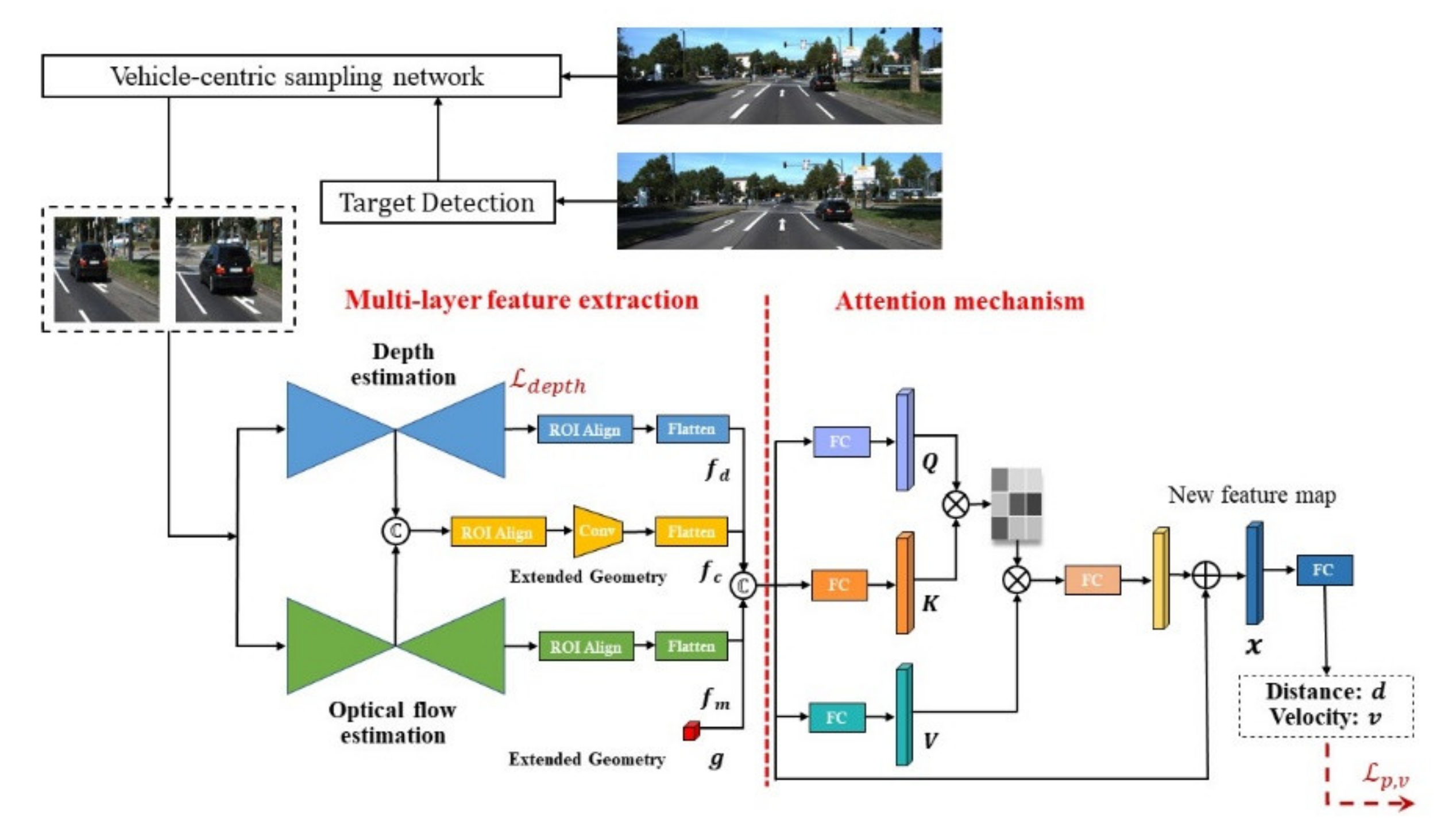
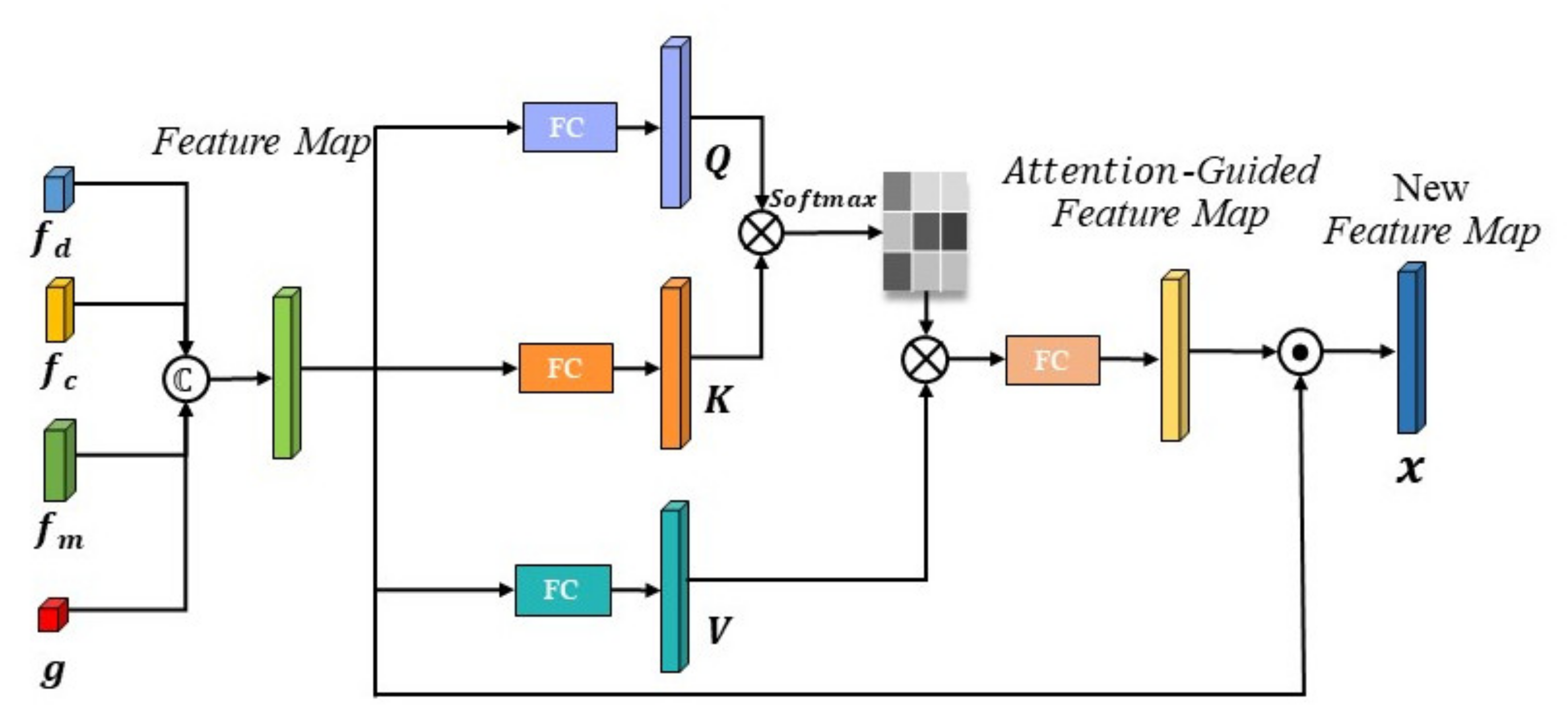
3. Method
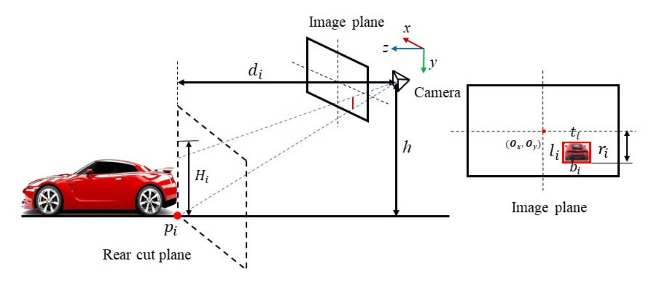
3.1. Geometric Cues and Odometry Models
3.2. Geometric Cues and Speed Models
4. Experimental Validation of Distance–Velocity Estimation Network
- Abs relative difference (AbsRel):
- 2.
- Squared relative difference (SqRel):
- 3.
- Root mean square error (RMSE):
- 4.
- Root mean square logarithmic error (RMSlog):
- 5.
- Accuracy:
- 6.
- Mean squared error (MSE):
4.1. Experimental Validation of the Tusimple Dataset
4.2. Experimental Validation of KITTI Dataset
4.2.1. Analysis of Performance Indicators
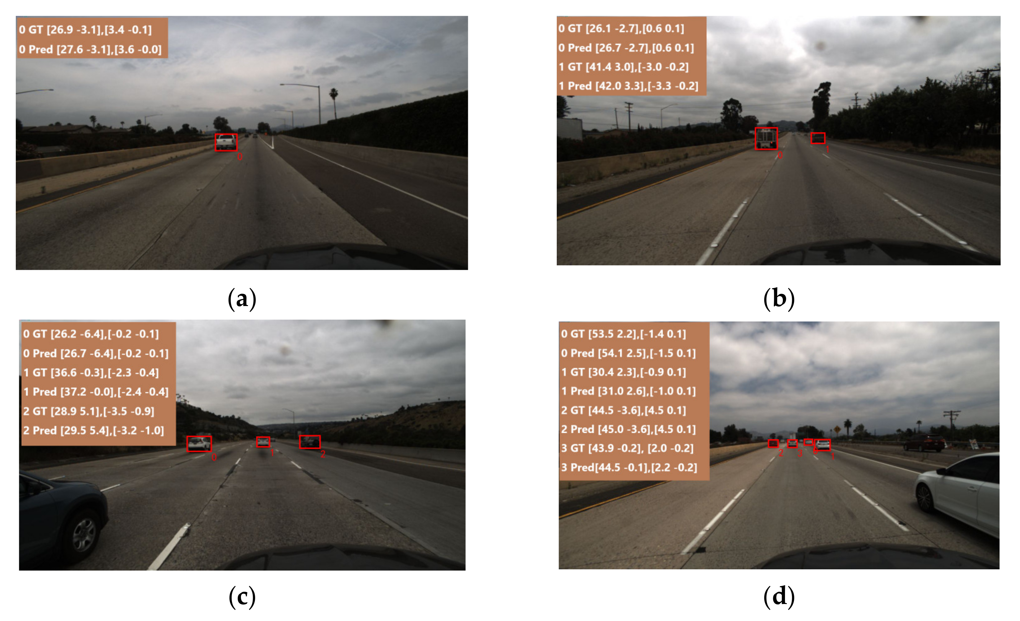
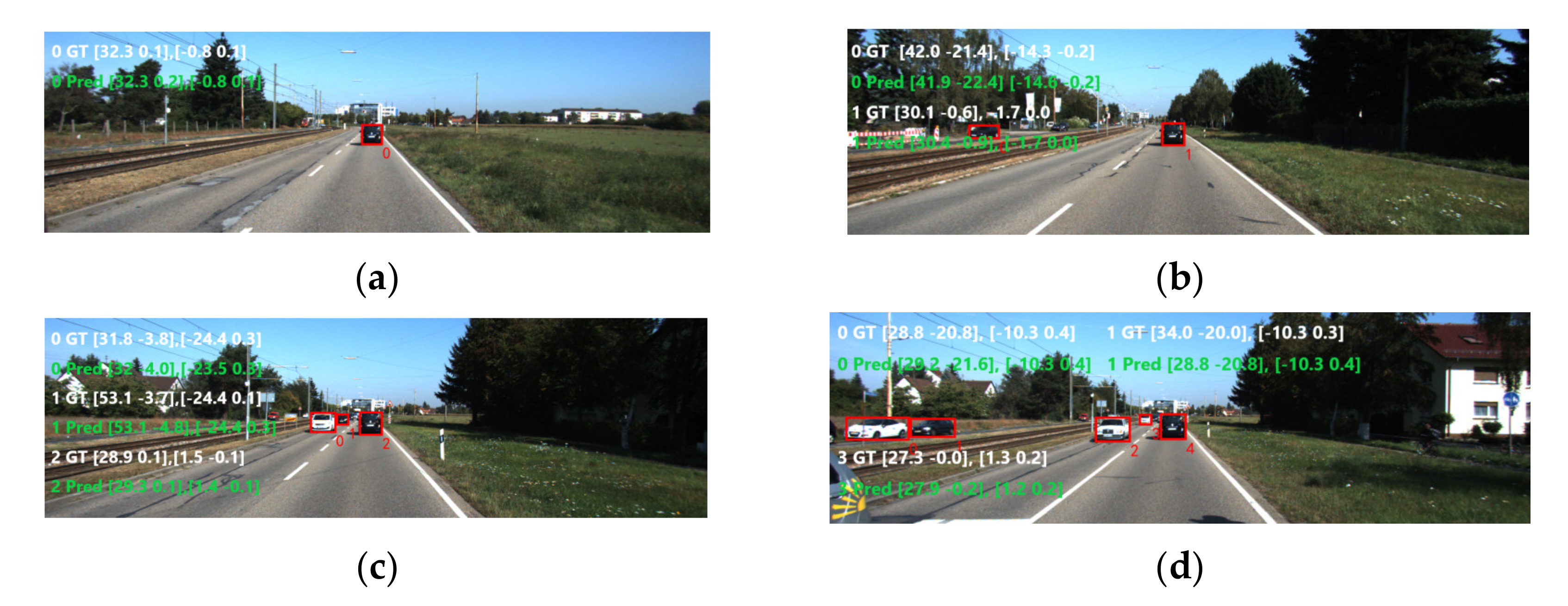
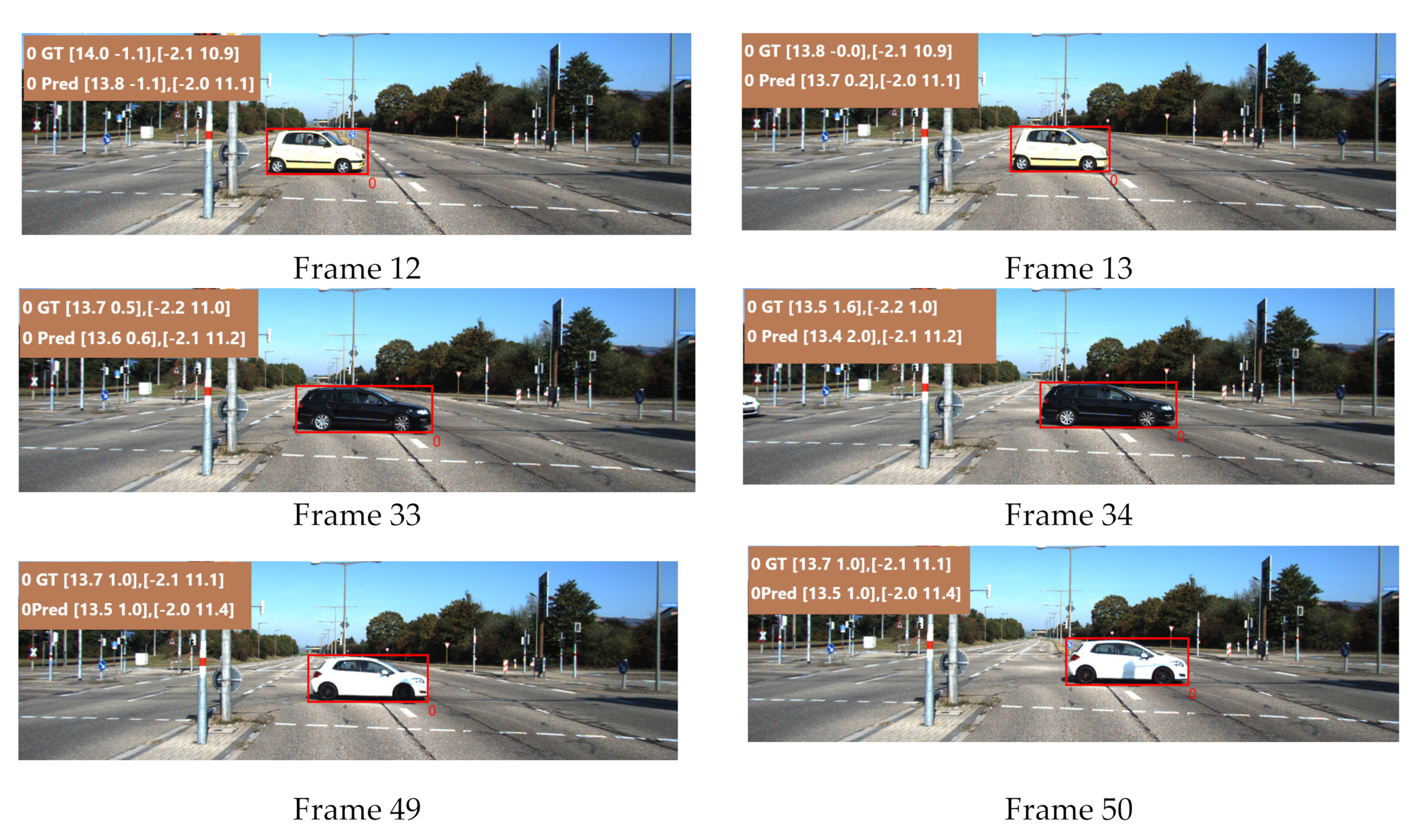
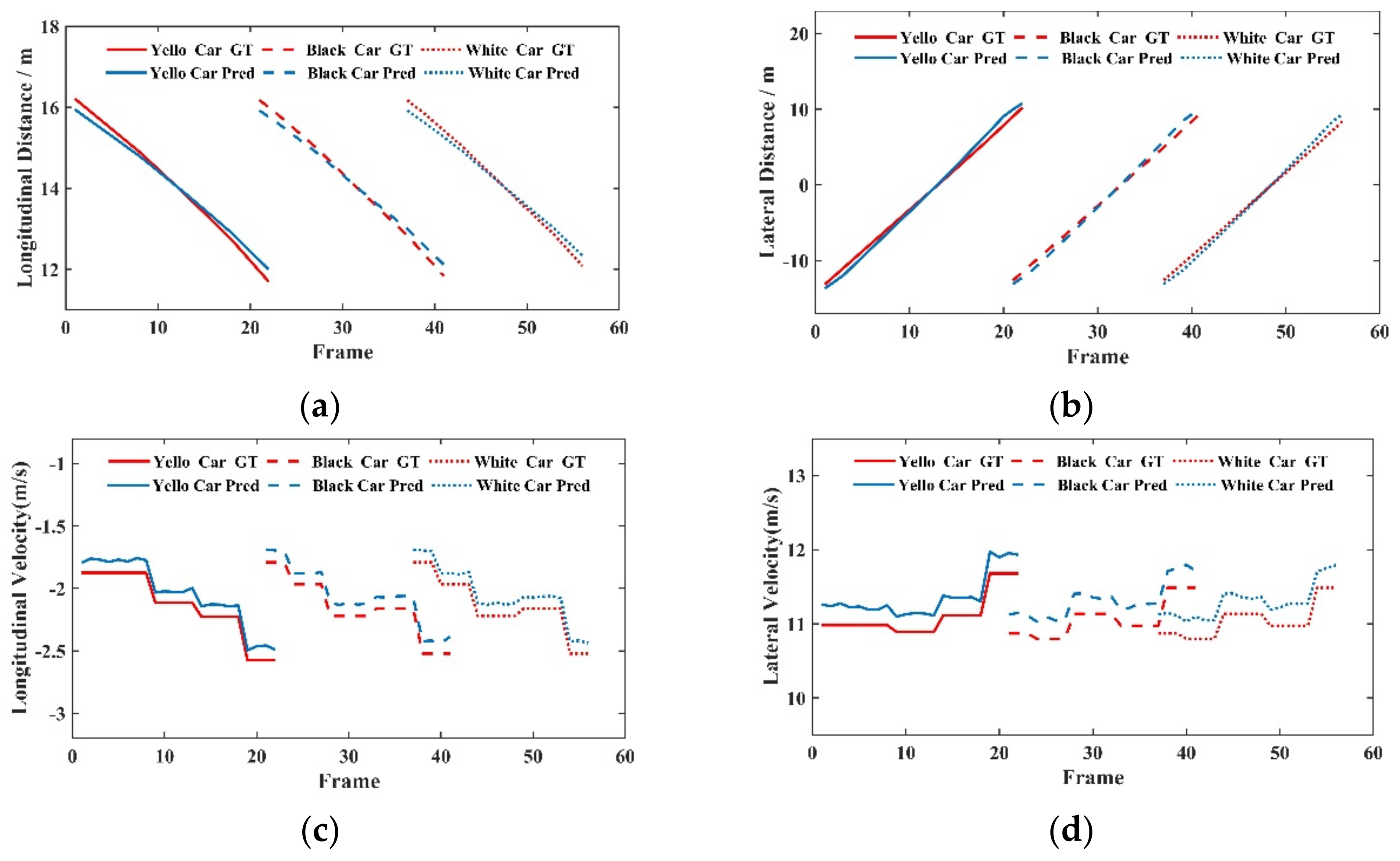
4.2.2. Qualitative Visualization Analysis
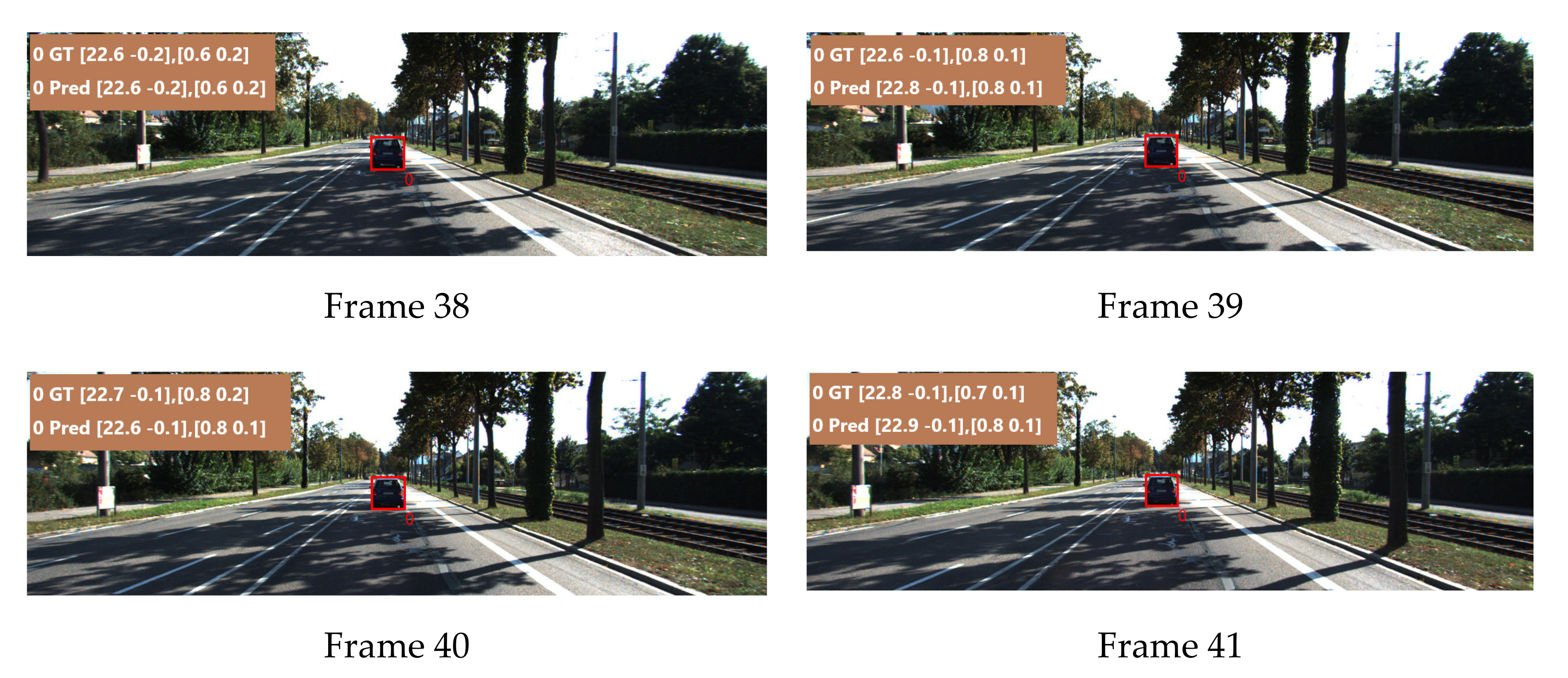
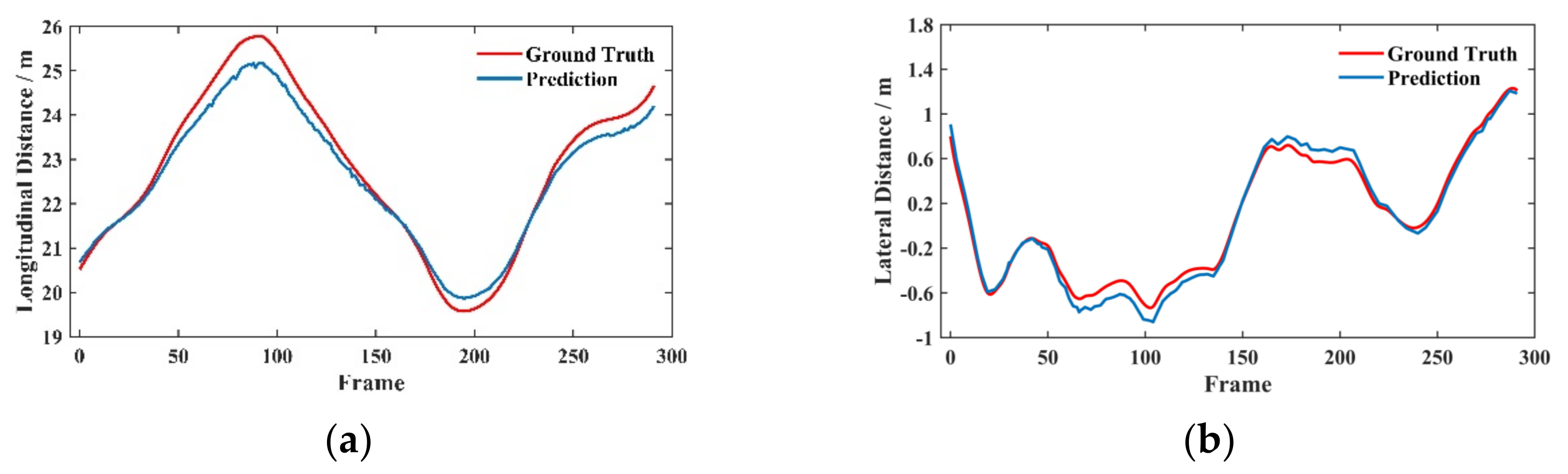
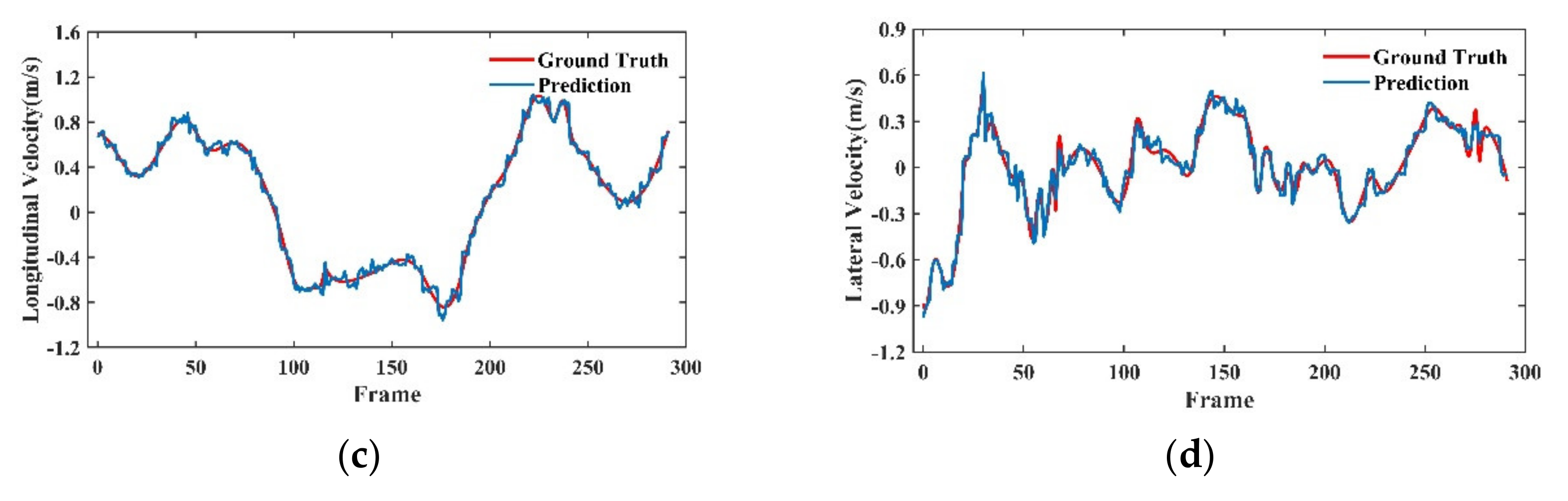
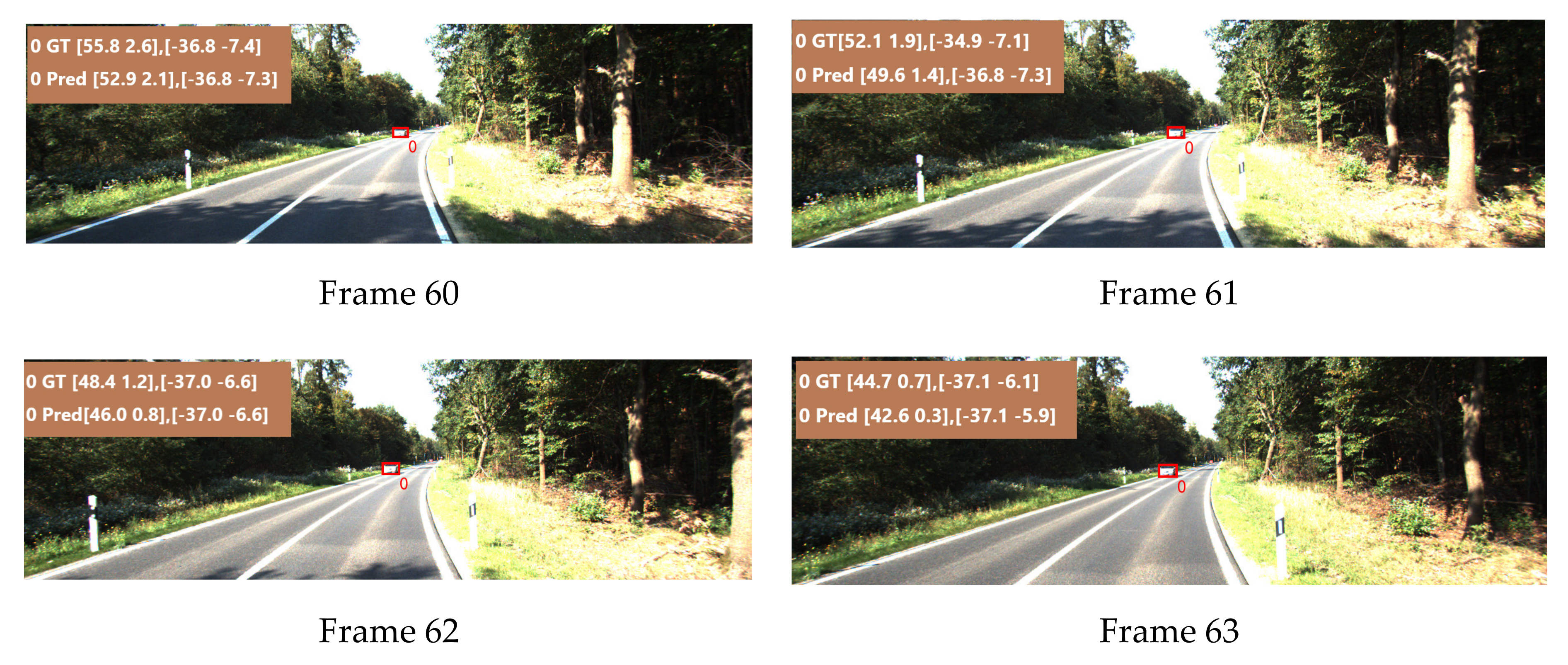
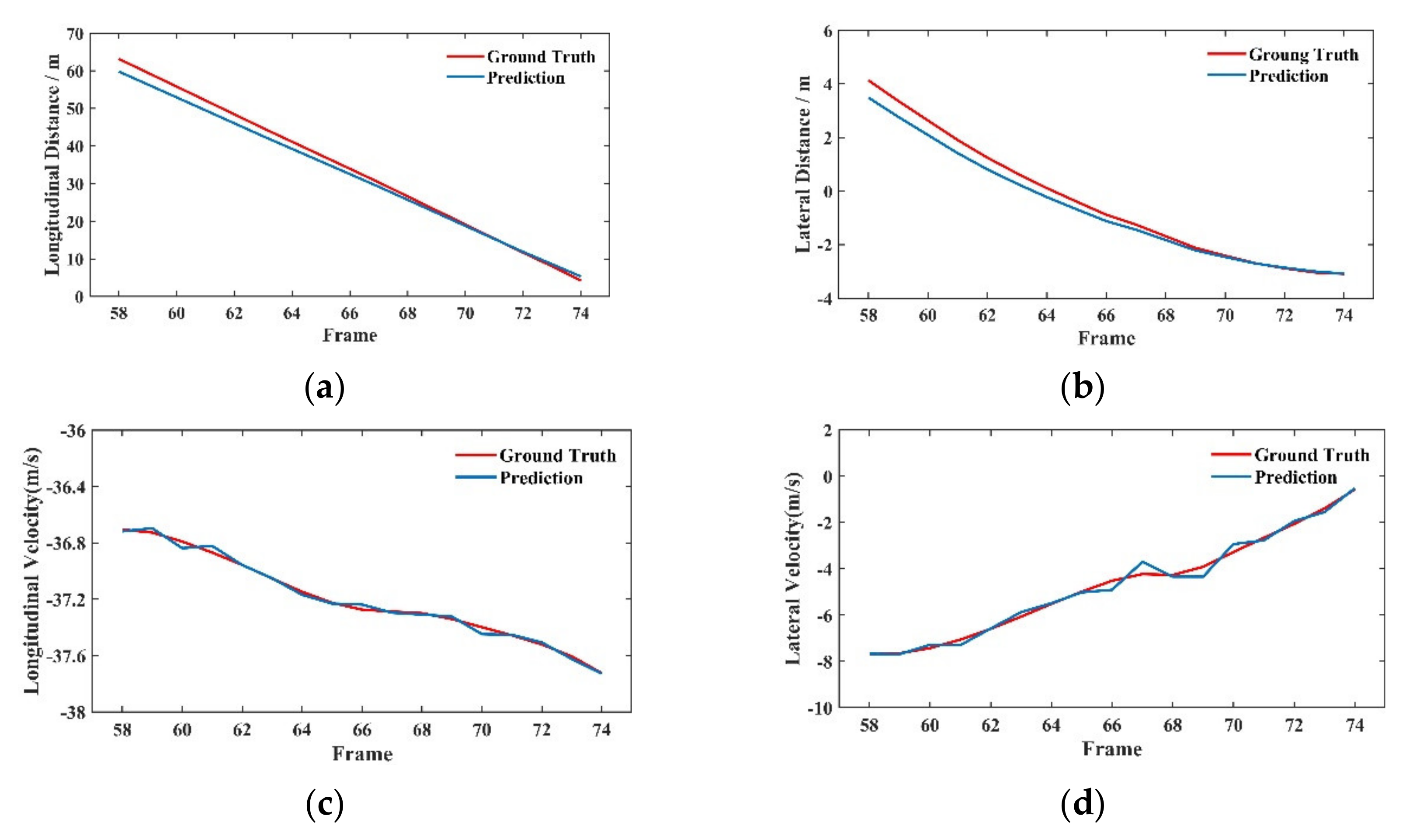
4.2.3. Visualization Analysis under Different Working Conditions
5. Discussion and Conclusions
Author Contributions
Funding
Institutional Review Board Statement
Informed Consent Statement
Data Availability Statement
Acknowledgments
Conflicts of Interest
References
- Hasirlioglu, S.; Riener, A.; Huber, W.; Wintersberger, P. Effects of Exhaust Gases on Laser Scanner Data Quality at Low Ambient Temperatures. In Proceedings of the 2017 IEEE Intelligent Vehicles Symposium (IV), Los Angeles, CA, USA, 11–14 June 2017. [Google Scholar]
- Fascista, A.; Ciccarese, G.; Coluccia, A.; Ricci, G. Angle of Arrival-Based Cooperative Positioning for Smart Vehicles. IEEE Trans. Intell. Transp. Syst. 2017, 19, 2880–2892. [Google Scholar] [CrossRef]
- Shin, J.; Sunwoo, M. Vehicle Speed Prediction Using a Markov Chain With Speed Constraints. IEEE Trans. Intell. Transp. Syst. 2018, 20, 3201–3211. [Google Scholar] [CrossRef]
- Redmon, J.; Divvala, S.; Girshick, R.; Farhadi, A. You Only Look Once: Unified, Real-Time Object Detection. In Proceedings of the IEEE Conference on Computer Vision and Pattern Recognition, Las Vegas, NV, USA, 27–30 June 2016. [Google Scholar]
- Ren, S.; He, K.; Girshick, R.; Sun, J. Faster R-CNN: Towards Real-Time Object Detection with Region Proposal Networks. Adv. Neural Inf. Process. Syst. 2015, 28, 28,1137–1149. [Google Scholar] [CrossRef] [PubMed] [Green Version]
- Fischer, P.; Dosovitskiy, A.; Ilg, E.; Häusser, P.; Hazırbaş, C.; Golkov, V.; van der Smagt, P.; Cremers, D.; Brox, T. FlowNet: Learning Optical Flow with Convolutional Networks. arXiv 2015, arXiv:1504.06852. [Google Scholar]
- Sun, D.; Yang, X.; Liu, M.Y.; Kautz, J. PWC-Net: CNNs for Optical Flow Using Pyramid, Warping, and Cost Volume. In Proceedings of the IEEE Conference on Computer Vision and Pattern Recognition, Salt Lake City, UT, USA, 18–23 June 2018. [Google Scholar]
- Bian, J.; Li, Z.; Wang, N.; Zhan, H.; Shen, C.; Cheng, M.M.; Reid, I. Unsupervised Scale-consistent Depth and Ego-motion Learning from Monocular Video. Adv. Neural Inf. Process. Syst. 2019, 32, 49–65. [Google Scholar]
- Fu, H.; Gong, M.; Wang, C.; Batmanghelich, K.; Tao, D. Deep Ordinal Regression Network for Monocular Depth Estimation. In Proceedings of the IEEE Conference on Computer Vision and Pattern Recognition, Salt Lake City, UT, USA, 18–23 June 2018. [Google Scholar]
- Menze, M.; Geiger, A. Object scene flow for autonomous vehicles in Computer Vision & Pattern Recognition. In Proceedings of the IEEE Conference on Computer Vision and Pattern Recognition, Boston, MA, USA, 7–12 June 2015. [Google Scholar]
- Ma, W.C.; Wang, S.; Hu, R.; Xiong, Y.; Urtasun, R. Deep Rigid Instance Scene Flow. In Proceedings of the IEEE/CVF Conference on Computer Vision and Pattern Recognition, Long Beach, CA, USA, 15–20 June 2019. [Google Scholar]
- Vogel, C.; Schindler, K.; Roth, S. 3D Scene Flow Estimation with a Piecewise Rigid Scene Model. Int. J. Comput. Vis. 2015, 115, 1–28. [Google Scholar] [CrossRef]
- Tran, M.T.; Dinh-Duy, T.; Truong, T.D.; Ton-That, V.; Do, T.N.; Luong, Q.A.; Nguyen, T.A.; Nguyen, V.T.; Do, M.N. Traffic Flow Analysis with Multiple Adaptive Vehicle Detectors and Velocity Estimation with Landmark-Based Scanlines. In Proceedings of the IEEE Conference on Computer Vision and Pattern Recognition Workshops, Salt Lake City, UT, USA, 18–22 June 2018. [Google Scholar]
- Kampelmühler, M.; Müller, M.G.; Feichtenhofer, C. Camera-based vehicle velocity estimation from monocular video. arXiv 2018, arXiv:1802.07094. [Google Scholar]
- Hirschm, H. Stereo Processing by Semiglobal Matching and Mutual Information. IEEE Trans. Pattern Anal. Mach. Intell. 2007, 30, 328–341. [Google Scholar] [CrossRef] [PubMed]
- Li, B.; Shen, C.; Dai, Y.; Van Den Hengel, A.; He, M. Depth and surface normal estimation from monocular images using regression on deep features and hierarchical CRFs. In Proceedings of the IEEE Conference on Computer Vision and Pattern Recognition, Boston, MA, USA, 7–12 June 2015. [Google Scholar]
- Eigen, D.; Puhrsch, C.; Fergus, R. Depth Map Prediction from a Single Image using a Multi-Scale Deep Network. In Proceedings of the 28th Conference on Neural Information Processing Systems (NIPS), Montreal, Canada, 8–13 December 2014. [Google Scholar]
- Lee, J.H.; Heo, M.; Kim, K.R.; Kim, C.S. Single-Image Depth Estimation Based on Fourier Domain Analysis. In Proceedings of the IEEE Conference on Computer Vision and Pattern Recognition, Salt Lake City, UT, USA, 18–23 June 2018. [Google Scholar]
- Li, J.; Klein, R.; Yao, A. Two-Streamed Network for Estimating Fine-Scaled Depth Maps from Single RGB Images. In Proceedings of the IEEE International Conference on Computer Vision, Venice, Italy, 22–29 October 2017. [Google Scholar]
- Laina, I.; Rupprecht, C.; Belagiannis, V.; Tombari, F.; Navab, N. Deeper Depth Prediction with Fully Convolutional Residual Networks. In Proceedings of the 2016 Fourth international conference on 3D vision (3DV), Stanford, CA, USA, 25–28 October 2016. [Google Scholar]
- Hu, J.; Ozay, M.; Zhang, Y.; Okatani, T. Revisiting Single Image Depth Estimation: Toward Higher Resolution Maps with Accurate Object Boundaries. In Proceedings of the 2019 IEEE Winter Conference on Applications of Computer Vision (WACV), Waikoloa Village, HI, USA, 7–11 January 2019. [Google Scholar]
- Liu, F.; Shen, C.; Lin, G. Deep Convolutional Neural Fields for Depth Estimation from a Single Image. In Proceedings of the IEEE Conference on Computer Vision and Pattern Recognition, Boston, MA, USA, 7–12 June 2015. [Google Scholar]
- Xu, D.; Ricci, E.; Ouyang, W.; Wang, X.; Sebe, N. Multi-Scale Continuous CRFs as Sequential Deep Networks for Monocular Depth Estimation. In Proceedings of the IEEE Conference on Computer Vision and Pattern Recognition, Honolulu, HI, USA, 21–26 July 2017. [Google Scholar]
- Rajagopalan, A.N.; Chaudhuri, S.; Mudenagudi, U. Depth Estimation and Image Restoration Using Defocused Stereo Pairs. IEEE Trans. Pattern Anal. Mach. Intell. 2004, 26, 1521–1525. [Google Scholar] [CrossRef] [PubMed]
- Saxena, A.; Chung, S.; Ng, A. Learning Depth from Single Monocular Images. Adv. Neural Inf. Process. Syst. 2005, 18, 1161–1168. [Google Scholar]
- Saxena, A.; Sun, M.; Ng, A.Y. Make3D: Learning 3D Scene Structure from a Single Still Image. IEEE Trans. Pattern Anal. Mach. Intell. 2008, 31, 824–840. [Google Scholar] [CrossRef] [PubMed] [Green Version]
- Karsch, K.; Liu, C.; Kang, S.B. Depth Extraction from Video Using Non-parametric Sampling. In Proceedings of the European Conference on Computer Vision, Florence, Italy, 7–13 October 2012; Springer: Berlin/Heidelberg, Germany, 2012. [Google Scholar]
- Song, S.; Chandraker, M.; Guest, C.C. High Accuracy Monocular SFM and Scale Correction for Autonomous Driving. IEEE Trans. Pattern Anal. Mach. Intell. 2015, 38, 730–743. [Google Scholar] [CrossRef] [PubMed]
- Song, S.; Chandraker, M. Robust Scale Estimation in Real-Time Monocular SFM for Autonomous Driving. In Proceedings of the IEEE Conference on Computer Vision and Pattern Recognition, Columbus, OH, USA, 23–28 June 2014. [Google Scholar]
- Szeliski, R. Computer Vision: Algorithms and Applications (Texts in Computer Science); Springer Science and Business Media: New York, NY, USA, 2010. [Google Scholar]
- Eigen, D.; Fergus, R. Predicting Depth, Surface Normals and Semantic Labels with a Common Multi-Scale Convolutional Architecture. In Proceedings of the International Conference on Computer Vision (ICCV), Santiago, Chile, 7-13 December 2015. [Google Scholar]
- Atapour-Abarghouei, A.; Breckon, T.P. Monocular Segment-Wise Depth: Monocular Depth Estimation Based on a Semantic Segmentation Prior. In Proceedings of the 2019 IEEE International Conference on Image Processing (ICIP), Taipei, Taiwan, 22–25 September 2019. [Google Scholar]
- Moukari, M.; Picard, S.; Simon, L.; Jurie, F. Deep multi-scale architectures for monocular depth estimation. In Proceedings of the 2018 25th IEEE International Conference on Image Processing (ICIP), Athens, Greece, 7–10 October 2018. [Google Scholar]
- Song, C.; Qi, C.; Song, S.; Xiao, F. Unsupervised Monocular Depth Estimation Method Based on Uncertainty Analysis and Retinex Algorithm. Sensors 2020, 20, 5389. [Google Scholar] [CrossRef] [PubMed]
- Zhe, T.; Huang, L.; Wu, Q.; Zhang, J.; Pei, C.; Li, L. Inter-Vehicle Distance Estimation Method Based on Monocular Vision Using 3D Detection. IEEE Trans. Veh. Technol. 2020, 69, 4907–4919. [Google Scholar] [CrossRef]
- Garg, R.; Bg, V.K.; Carneiro, G.; Reid, I. Unsupervised CNN for Single View Depth Estimation: Geometry to the Rescue; Springer: Cham, Switzerland, 2016. [Google Scholar]
- Godard, C.; Mac Aodha, O.; Brostow, G.J. Unsupervised Monocular Depth Estimation with Left-Right Consistency. In Proceedings of the IEEE Conference on Computer Vision and Pattern Recognition, Honolulu, HI, USA, 21–26 July 2017. [Google Scholar]
- Zhou, T.; Krahenbuhl, P.; Aubry, M.; Huang, Q.; Efros, A.A. Learning Dense Correspondence via 3D-guided Cycle Consistency. In Proceedings of the IEEE Conference on Computer Vision and Pattern Recognition, Las Vegas, NV, USA, 27–30 June 2016. [Google Scholar]
- Zhou, T.; Tulsiani, S.; Sun, W.; Malik, J.; Efros, A.A. View Synthesis by Appearance Flow. In Proceedings of the European Conference on Computer Vision, Amsterdam, The Netherlands, 11–14 October 2016; Springer: Cham, Switzerland, 2016. [Google Scholar]
- Yin, Z.; Shi, J. GeoNet: Unsupervised Learning of Dense Depth, Optical Flow and Camera Pose. In Proceedings of the IEEE Conference on Computer Vision and Pattern Recognition, Salt Lake City, UT, USA, 18–23 June 2018. [Google Scholar]
- Ilg, E.; Mayer, N.; Saikia, T.; Keuper, M.; Dosovitskiy, A.; Brox, T. FlowNet 2.0: Evolution of Optical Flow Estimation with Deep Networks. In Proceedings of the IEEE Conference on Computer Vision and Pattern Recognition, Honolulu, HI, USA, 21–26 July 2017.
- Song, Z.; Lu, J.; Zhang, T.; Li, H. End-to-end Learning for Inter-Vehicle Distance and Relative Velocity Estimation in ADAS with a Monocular Camera. In Proceedings of the 2020 IEEE International Conference on Robotics and Automation (ICRA), Paris, France, 31 May–31 August 2020. [Google Scholar]
- Huang, K.C.; Huang, Y.K.; Hsu, W.H. Multi-Stream Attention Learning for Monocular Vehicle Velocity and Inter-Vehicle Distance Estimation. arXiv 2021, arXiv:2110.11608. [Google Scholar]
- Redmon, J.; Farhadi, A. YOLOv3: An Incremental Improvement. arXiv 2018, arXiv:1804.02767. [Google Scholar]
- Mousavian, A.; Anguelov, D.; Flynn, J.; Kosecka, J. 3D Bounding Box Estimation Using Deep Learning and Geometry. In Proceedings of the IEEE conference on Computer Vision and Pattern Recognition, Honolulu, HI, USA, 21–26 July 2017. [Google Scholar]


| Literature | Model Structure | Main Contribution |
|---|---|---|
| Eigen et al. [17] | CNN | Used deep learning models for the first time |
| Lee et al. [18] | CNN | Optimizing the frequency domain |
| Li et al. [19] | CNN | Used gradient information for optimization |
| Laina et al. [20] | FCN | Proposed a new sampling module |
| Hu et al. [21] | FCN | Used multiscale information to improve |
| Liu et al. [22] | CNN | Random field step-by-step optimization |
| Xu et al. [23] | FCN | Optimized with continuity condition |
| Distance (m) | Close Range | Middle Range | Long Range | Total |
|---|---|---|---|---|
| Training Set | 166 | 943 | 333 | 1442 |
| Test Set | 29 | 247 | 99 | 375 |
| Method | Distance | Velocity | |||
|---|---|---|---|---|---|
| Rank1 [17] | - | 0.18 | 0.66 | 3.07 | 1.30 |
| Rank2 | - | 0.25 | 0.75 | 3.50 | 1.50 |
| Rank3 | - | 0.55 | 2.21 | 5.94 | 2.90 |
| Song et al. [34] (org) | 9.72 | 0.23 | 0.99 | 3.27 | 1.50 |
| Song et al. [34] (full) | 10.23 | 0.15 | 0.34 | 2.09 | 0.86 |
| Huang et al. [27] | 7.56 | 0.10 | 0.26 | 1.58 | 0.65 |
| Our Method | 5.659 | 0.077 | 0.196 | 1.217 | 0.496 |
| Index | Song et al. [34] (org) | Song et al. [34] (full) | Huang et al. [27] | Our Method |
|---|---|---|---|---|
| 0.037 | 0.041 | 0.034 | 0.038 | |
| 0.132 | 0.152 | 0.105 | 0.076 | |
| 2.700 | 2.894 | 2.416 | 1.993 | |
| 0.059 | 0.062 | 0.050 | 0.038 | |
| 0.989 | 0.987 | 0.997 | 0.997 | |
| 1.000 | 1.000 | 1.000 | 1.000 | |
| 1.000 | 1.000 | 1.000 | 1.000 |
| Vehicle ID | Distance (m) | Relative Velocity (m/s) | ||
|---|---|---|---|---|
| True Value | Predicted Value | True Value | Predicted Value | |
| A-0 | (26.9, −3.1) | (27.6, −3.1) | (3.4, −0.1) | (3.6, −0.0) |
| B-0 | (26.1, −2.7) | (26.7, −2.7) | (0.6, 0.1) | (0.6, 0.1) |
| B-1 | (41.4, 3.0) | (42.0, 3.3) | (−3.0, −0.2) | (−3.3, −0.2) |
| C-0 | (26.2, −6.4) | (26.7, −6.4) | (−0.2, −0.1) | (−0.2, −0.1) |
| C-1 | (36.6, −0.3) | (37.2, −0.0) | (−2.3, −0.4) | (−2.4, −0.4) |
| C-2 | (28.9, 5.1) | (29.5, 5.4) | (−3.5, −0.9) | (−3.2, −1.0) |
| D-0 | (53.5, 2.2) | (54.1, 2.5) | (−1.4, 0.1) | (−1.5, 0.1) |
| D-1 | (30.4, 2.3) | (31.0, 2.6) | (−0.9, 0.1) | (−1.0, 0.1) |
| D-2 | (44.5, −3.6) | (45.0, −3.6) | (4.6, 0.0) | (4.5, 0.1) |
| D-3 | (43.9, −0.2) | (44.5, −0.1) | (2.0, 0.0) | (2.2, −0.2) |
| Song et al. [34] | 0.29 | 0.93 | 1.57 | 0.94 |
| Huang et al. [27] | 0.23 | 0.67 | 0.96 | 0.62 |
| Our Method | 0.16 | 0.27 | 0.78 | 0.40 |
| Indicators | 3Dbbox [45] | DORN [9] | Unsfm [8] | Song et al. [34] | Huang et al. [27] | Our Method |
|---|---|---|---|---|---|---|
| 0.222 | 0.078 | 0.219 | 0.075 | 0.098 | 0.085 | |
| 1.863 | 0.505 | 1.924 | 0.474 | 0.444 | 0.375 | |
| 7.696 | 4.078 | 7.873 | 4.639 | 4.240 | 4.114 | |
| 0.228 | 0.179 | 0.338 | 0.124 | 0.127 | 0.108 | |
| 0.659 | 0.927 | 0.710 | 0.912 | 0.930 | 0.974 | |
| 0.966 | 0.985 | 0.886 | 0.996 | 0.998 | 0.997 | |
| 0.994 | 0.995 | 0.933 | 1.000 | 1.000 | 1.000 |
| Vehicle ID | Distance (m) | Relative Speed (m/s) | ||
|---|---|---|---|---|
| True Value | Predicted Value | True Value | Predicted Value | |
| A-0 | (32.3, −0.1) | (32.3, −0.2) | (−0.8, 0.1) | (−0.8, 0.1) |
| B-0 | (42.9, −21.4) | (41.9, −22.4) | (−14.3, −0.2) | (−14.6, −0.2) |
| B-1 | (30.1, −0.6) | (30.4, −0.9) | (−1.7, 0.0) | (−1.7, 0.0) |
| C-0 | (31.8, −3.8) | (30.5, −4.0) | (−24.4, 0.3) | (−23.5, 0.3) |
| C-1 | (53.1, −3.7) | (51.3, −4.7) | (−24.4, 0.1) | (−23.8, −0.1) |
| C-2 | (28.9, 0.1) | (29.3, −0.1) | (1.5, −0.1) | (1.4, −0.1) |
| D-0 | (28.8, −20.8) | (29.2, −21.6) | (−10.3, 0.4) | (−10.3, 0.4) |
| D-1 | (34.0, −20.0) | (33.9, 20.9) | (−10.2, 0.3) | (−9.9, 0.3) |
| D-2 | (25.9, −3.7) | (25.2, −3.8) | (−22.4, 0.0) | (−22.7, 0.1) |
| D-3 | (61.2, −4.2) | (58.4, −5.5) | (−24.0, 0.6) | (−23.4, 0.6) |
| D-4 | (27.3, −0.0) | (27.9, −0.2) | (1.3, 0.2) | (1.2, 0.2) |
| Deep Network | Optical Flow Network | Attention Mechanism | Fully Connected Layer | Total Time Consumption | |
|---|---|---|---|---|---|
| Hardware Time | GPU 8 ms | GPU 20 ms | GPU 0.4 ms | GPU 0.3 ms | GPU 30 ms |
Publisher’s Note: MDPI stays neutral with regard to jurisdictional claims in published maps and institutional affiliations. |
© 2022 by the authors. Licensee MDPI, Basel, Switzerland. This article is an open access article distributed under the terms and conditions of the Creative Commons Attribution (CC BY) license (https://creativecommons.org/licenses/by/4.0/).
Share and Cite
Qi, C.; Zhao, H.; Song, C.; Zhang, N.; Song, S.; Xu, H.; Xiao, F. Monocular Depth and Velocity Estimation Based on Multi-Cue Fusion. Machines 2022, 10, 396. https://doi.org/10.3390/machines10050396
Qi C, Zhao H, Song C, Zhang N, Song S, Xu H, Xiao F. Monocular Depth and Velocity Estimation Based on Multi-Cue Fusion. Machines. 2022; 10(5):396. https://doi.org/10.3390/machines10050396
Chicago/Turabian StyleQi, Chunyang, Hongxiang Zhao, Chuanxue Song, Naifu Zhang, Sinxin Song, Haigang Xu, and Feng Xiao. 2022. "Monocular Depth and Velocity Estimation Based on Multi-Cue Fusion" Machines 10, no. 5: 396. https://doi.org/10.3390/machines10050396