Article

Fundamental Design and Modelling of the Superconducting Magnet for the High-Speed Maglev: Mechanics, Electromagnetics, and Loss Analysis during Instability

1
School of Electrical and Information Engineering, Tianjin University, Tianjin 300072, China
2
Clare Hall, University of Cambridge, Cambridge CB3 9AL, UK
3
Department of Engineering, University of Cambridge, Cambridge CB3 0FA, UK
4
Faculty of Engineering and Information Technology, University of Technology Sydney, Sydney, NSW 2007, Australia
5
School of Electrical and Information Engineering, The University of Sydney, Sydney, NSW 2006, Australia
*
Authors to whom correspondence should be addressed.
These authors contributed equally to this work.
Machines 2022, 10(2), 113; https://doi.org/10.3390/machines10020113
Submission received: 21 December 2021 / Revised: 27 January 2022 / Accepted: 31 January 2022 / Published: 3 February 2022
(This article belongs to the Special Issue Feature Papers to Celebrate the First Impact Factor of Machines)

Abstract

:
The high-temperature superconductor (HTS) has been recognised as one of the most up-and-coming materials thanks to its superior electromagnetic performance (e.g., zero resistance). For a high-speed maglev, the HTS magnet can be the most crucial component because it is in charge of both the levitation and the propulsion of the maglev. Therefore, a fundamental study of HTS magnets for maglev is crucial. This article presents the fundamental design and modelling of the superconducting magnet for a high-speed maglev, including mechanics, electromagnetics, and loss analysis during instability. First, the measurements of the superconducting wire were performed. The HTS magnet was primarily designed and modelled to fulfil the basic electromagnetic requirements (e.g., magnetic field) in order to drive the maglev at a high speed. The modelling was verified by experimental tests on a scale-down HTS magnet. A more professional model using the H-formulation based on the finite element method (FEM) was built to further investigate some deeper physical phenomenon of the HTS magnet (e.g., current density and loss behaviours), particularly in situations where the high-speed maglev is in the normal steady state or encountering instability.

1. Introduction

Down through the ages, high-speed travel is undoubtedly one of the most important aspects of transportation technology throughout the civilisation of human beings. In 1804, the world’s first steam-powered railway train (locomotive) was run by R. Trevithick near the Merthyr Tydfil in South Wales [1]. Since then, railway transportation has been developed remarkably and become the safest and most convenient way to transport passengers and goods domestically and internationally. The maglev (magnetic levitation) train was first patented by H. Kemper in 1937 [2] and has attracted a lot of attentions. For traditional linear motors used in maglev, the excitation winding is very difficult to improve the efficiency of the power factor due to the limitation of the current and loss in the conductor. However, the strong current-carrying capacity of a superconducting magnet can solve this problem. Combining the superconductor technology with the maglev has made it even more powerful [3], and the superconducting maglev based on the low-temperature superconductor (LTS) has progressed well worldwide [4].
With the rapid development of the high-temperature superconductor (HTS), many large-scale HTS applications have already moved from research labs to industrial applications [5]. The application of superconducting magnets used for magnetic levitation has ushered in a perfect opportunity. In the 1990s, scientists and engineers started to develop HTS maglevs. The first man-loading HTS maglev was shown in 2000 [6]. Since then, different configurations of HTS maglev have been proposed in Russia [7], Japan [8], Germany [9], Italy [10], China [11], and Brazil [12]. In 2005, a full-size HTS maglev was run in the Yamanashi Maglev Test Line, and it achieved a top speed of 553 km/h [13].
Although a certain amount of research and tests of HTS maglevs and their magnets have already been carried out [14,15,16,17,18], to the best of our search on literatures, some in-depth aspects are still missing. There is no fundamental study showing the design of HTS magnets for high-speed maglevs, covering simultaneously the mechanics, electromagnetics, and loss analysis when the HTS maglev has instability. This article presents these missing but crucial aspects with a fundamental study on the magnetic field, force, critical current, current density, and loss when the superconducting maglev is running normally or encountering instability, which is important for the safe and reliable operation of the high-speed maglev.

2. HTS Magnet Design and Characterisation

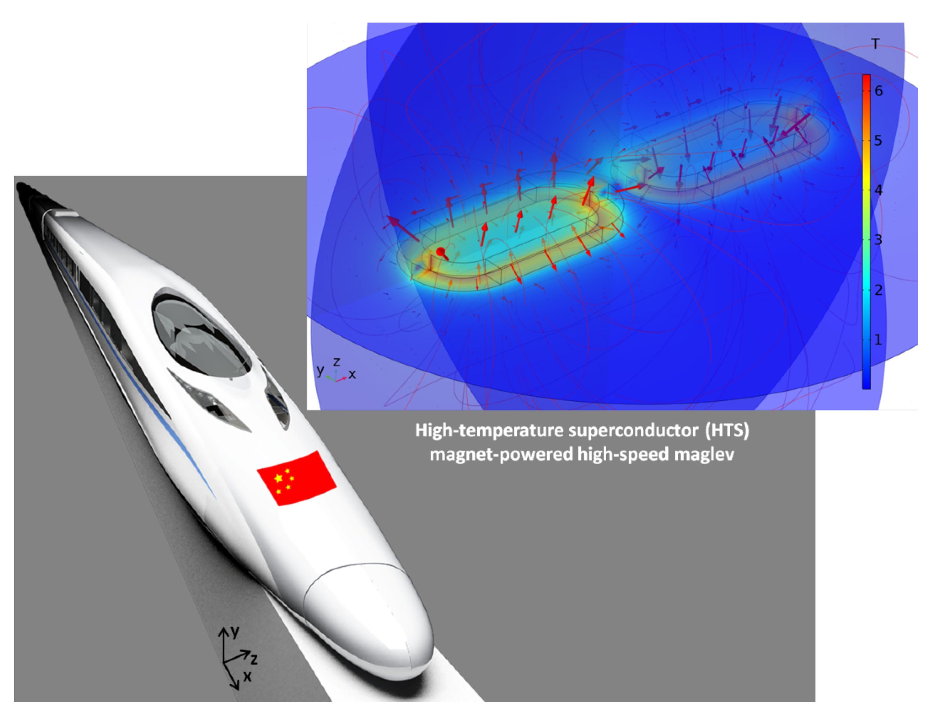
2.1. Introduction of the HTS Magnet for High-Speed Maglev

Figure 1 shows a high-speed maglev for a proposed top speed over 600 km/h (conceptual design), its HTS magnet, and the corresponding magnetic fields. The HTS magnet is the key component of maglev as it is in charge of both the levitation and the propulsion of the maglev. For a high-speed maglev with top speed over 550 km/h, the magnet design should at least meet or even surpass the basic requirement of the magnetomotive force (750 kA) [13]. Figure 1 shows the overall magnetic field pattern with opposite orientations (+ and −, in the z-direction) produced by a pair of magnets. A more detailed design process and specific values are shown in the following paragraphs.

2.2. Superconducting Electrodynamic Suspension (EDS) Using the HTS Magnet

How to realise the suspension using the superconducting technology is a key point for the HTS maglev. In this article, the HTS magnet is designed for the maglev type of superconducting electrodynamic suspension (EDS). Figure 2 shows the working principle of the superconducting EDS of the HTS maglev, HTS magnet, 8-shape coil, and equivalent circuit.
When an HTS coil passes through the 8-shape coil in the x-direction, according to Faraday’s law, the electromagnetic induction can be calculated as [19]:
e 1 = N 1 d ϕ 1 d t = d ( M s 1 I s ) d ( x / v x ) = I s v x M s 1 x
e 2 = N 1 d ϕ 2 d t = d ( M s 2 I s ) d ( x / v x ) = I s v x M s 2 x
e 1 e 2 = 2 R i + 2 ( L M 12 ) d i d t
where e1 and e2 are the electromotive force (EMF) induced by the interaction in the upper coil 1 and lower coil 2, and Φ1 and Φ2 are the corresponding magnetic fluxes from the HTS magnet, respectively. N1 is the turns of the 8-shape coil. R and L are the resistance and self-inductance of the upper or lower coils, and M12 is the mutual inductance between the upper and lower coils. Ms1 and Ms2 are the mutual inductances between the HTS magnet and the upper coil 1 and lower coil 2. Is is the current of the SC coil. vx is the moving velocity of the HTS magnet. If the HTS magnets interact with an array of 8-shape coils simultaneously, one can derive:
[ R 0 0 0 0 R 0 0 0 0 0 0 0 0 R ] [ i 1 i 2 i n ] + [ L 1 , 1 L 1 , n + 1 L 1 , 2 L 1 , n + 2 L 1 , n L 1 , 2 n L 2 , 1 L 2 , n + 1 L 2 , 2 L 2 , n + 2 L 2 , n L 2 , 2 n L n , 1 L n , n + 1 L n , n L n , 2 n ] × d d t [ i 1 i 2 i n ] = [ G 1 , 1 G n + 1 , 1 G 1 , 2 G n + 1 , 2 G 1 , M G n + 1 , M G 2 , 1 G n + 2 , 1 G 2 , 2 G n + 2 , 2 G 2 , M G n + 2 , M G n , 1 G 2 n , 1 G n , M G 2 n , M ] × [ I s 1 I s 2 I s M ] v x 2
where Lij is the mutual inductance between the ith and jth guideway loop coils. m and n are the labels of the HTS magnets and 8-shape coils. Gi,k is the mutual inductance between the HTS magnet and the ith 8-shape coil, and Gn+i,k is the mutual inductance between the HTS magnet and the (n + i)th 8-shape coil, k = 1 ~ m. ii is the induced current of the jth 8-shape coil, i = 1 ~ n and j = 1 ~ 2n. Isk is the current of the kth HTS magnet. The HTS magnets moving along the x-axis can induce three components (fx, fy, and fz) of the electromagnetic force:
f x = i = 1 n k = 1 M I s k i i ( M s i , k x M s n + i , k x )
f y = i = 1 n k = 1 M I s k i i ( M s i , k y M s n + i , k y )
f z = i = 1 n k = 1 M I s k i i ( M s i , k z M s n + i , k z )
It can be found that at the beginning, the levitation force fast increases with the increasing speed, but then the levitation force slowly increases and is saturated after reaching a certain speed. The reason is that although the induced voltage in the 8-shape-coil goes up with the increasing speed, the overall impedance of the coil also rises due to the frequency and skin effect [19].

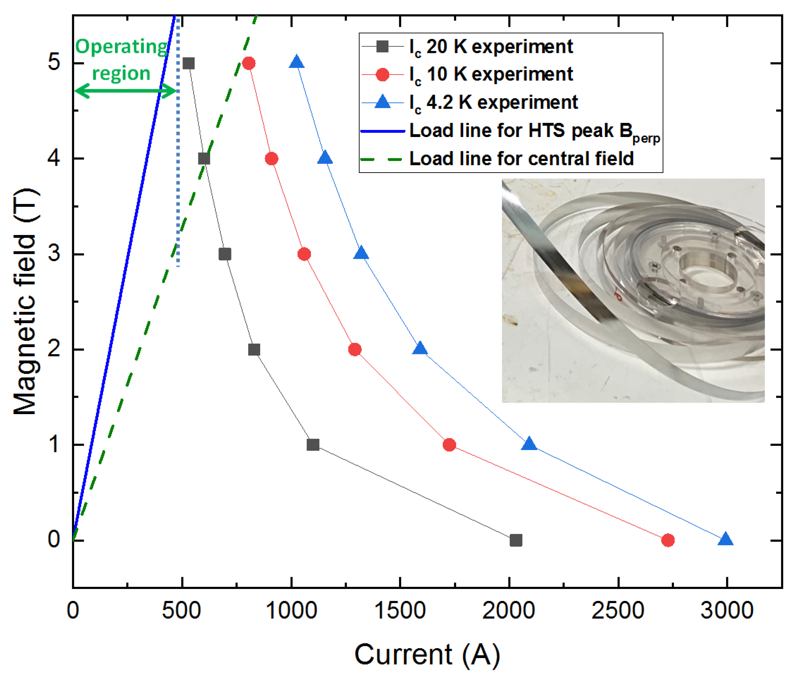
2.3. Geometry and Operating Current of the HTS Magnet

A single HTS magnet is mounted with three racetrack double-pancake (DP) coils, each having 2 × 500 turns of HTS wires. The geometrical size of a single HTS magnet is 1050 mm × 510 mm × 72 mm, which can well fit a real-size high-speed maglev. The detailed parameters of the HTS magnet are listed in Table 1.
In order to meet the requirements of the magnetic field and force for maglev, selecting the proper operating current of the HTS magnet is really crucial. The critical current (Ic) of the superconductor means the threshold of the maximum current that the superconductor can carry without perceptible loss, and if it is over Ic, the superconductor will become massively resistive and thus generate a great amount of loss. The HTS wires have the high aspect ratio of geometry and the anisotropic characteristic of Ic under different magnetic fields. Ic would significantly decrease if the HTS wire is exposed to a strong magnetic field. Therefore, the fundamental measurements of Ic in different magnetic fields and operating temperatures should be performed, and these experimental results are fairly important to achieve the realistic modelling.
The HTS wire proposed for the HTS magnet was the 12 mm wide rare-earth barium copper oxide (REBCO) tape made by Shanghai Superconductor Technology Co. Ltd., with an overall thickness of approximately 200 µm (if with the additional insulation layer made by the epoxy encapsulation). The critical current was measured in the presence of different values of the magnetic field (perpendicular direction to the wide surface of the tape) with different temperatures at 4.2, 10, and 20 K. In Figure 3, one load line is for the HTS magnet central field; the other load line is for the peak perpendicular field component, which is more relevant to the real operating current, because the cross point with the critical current curves is where the maximum operating current takes place. For example, for the temperature 20 K, the maximum operating current is around 480 A. To make a safe margin, the operating current can be set to 350–360 A at approximately 20 K.

2.4. Magnetic Field and Force of the HTS Magnet

To investigate more physical details of the electromagnetic/force analysis of the HTS magnet in Figure 1, Figure 4 shows the magnetic field and force per unit volume in the x-, y-, and z-direction on the top surface of the HTS magnet, with an operating current of 350 A. The modelling was performed by using the “magnetic field, mf” module in COMSOL:
× H = J
× A = B
μ 0 ( M + H ) = B
Equation (8) is the Ampere’s law, where H is the magnetic field intensity, and J is the electric current density. Equation (9) is the definition of magnetic potential, where B is the magnetic flux density, and A is the magnetic potential. Equation (10) is the constitutive relationship, where M is the magnetisation, and µ0 is the vacuum permeability. For different properties in the HTS tapes (e.g., non-magnetic materials or magnetic materials, such as the magnetic substrates), the magnetisation behaviours will be different as governed by.
σ v × B + J e = J
In the magnetostatic relation, v is the velocity of the conductor, σ the electrical conductivity, and Je an externally generated current density. Combining (8), (9), (10), and (11), one obtains the governing equation of the mf module as:
× ( μ 0 1 × A M ) σ v × ( × A ) = J e
It can be seen that for the x-direction, the strongest magnetic field (−4.04 T and +4.15 T) and strongest force (−6.88 × 10⁸ N/m3 and 6.90 × 10⁸ N/m3) appear on the opposite sides of the HTS magnet, which reveals that the strongest expansion force is located in the inner part of the HTS magnet. For the y-direction, the strongest magnetic field (−4.14 T and +4.14 T) and the strongest force (−6.25 × 10⁸ N/m3 and 6.26 × 10⁸ N/m3) have a fairly similar tendency as the x-direction, which suggests that the strongest expansion force is located all the way through the inner perimeter of the HTS magnet. For the z-direction, the strongest magnetic field (−4.73 T and +4.74 T) is in the opposite poles of the pair magnet (close to the inner perimeter), and strongest force (6.02 × 10⁸ N/m3) is on the top surface of the HTS magnet, which shows that the lateral force in the same direction of the pair magnet should be carefully considered.
The magnetic field component in the z-direction of the HTS magnet is one of the most important indexes, as the sufficient z-direction magnetic strength is the key to achieve the strong propulsion force and high speed of the maglev. Figure 5 shows the magnetic flux density in the z-direction (Bz) along the reference lines at 50, 100, and 150 mm above the HTS magnets, with an operating current of 350 A. Compared with the maximum magnetic strength in the z-direction (Bz) of 4.74 T shown in Figure 4c, the peak magnetic strength decays to 2.49, 1.68, and 1.32 T, with the reference lines at 50, 100, and 150 mm above the HTS magnets. Compared with the results in [13], the magnetic field patterns in the z-direction (Bz) above the HTS magnets are already strong enough to create a strong propulsion and realise the high-speed running for the maglev.

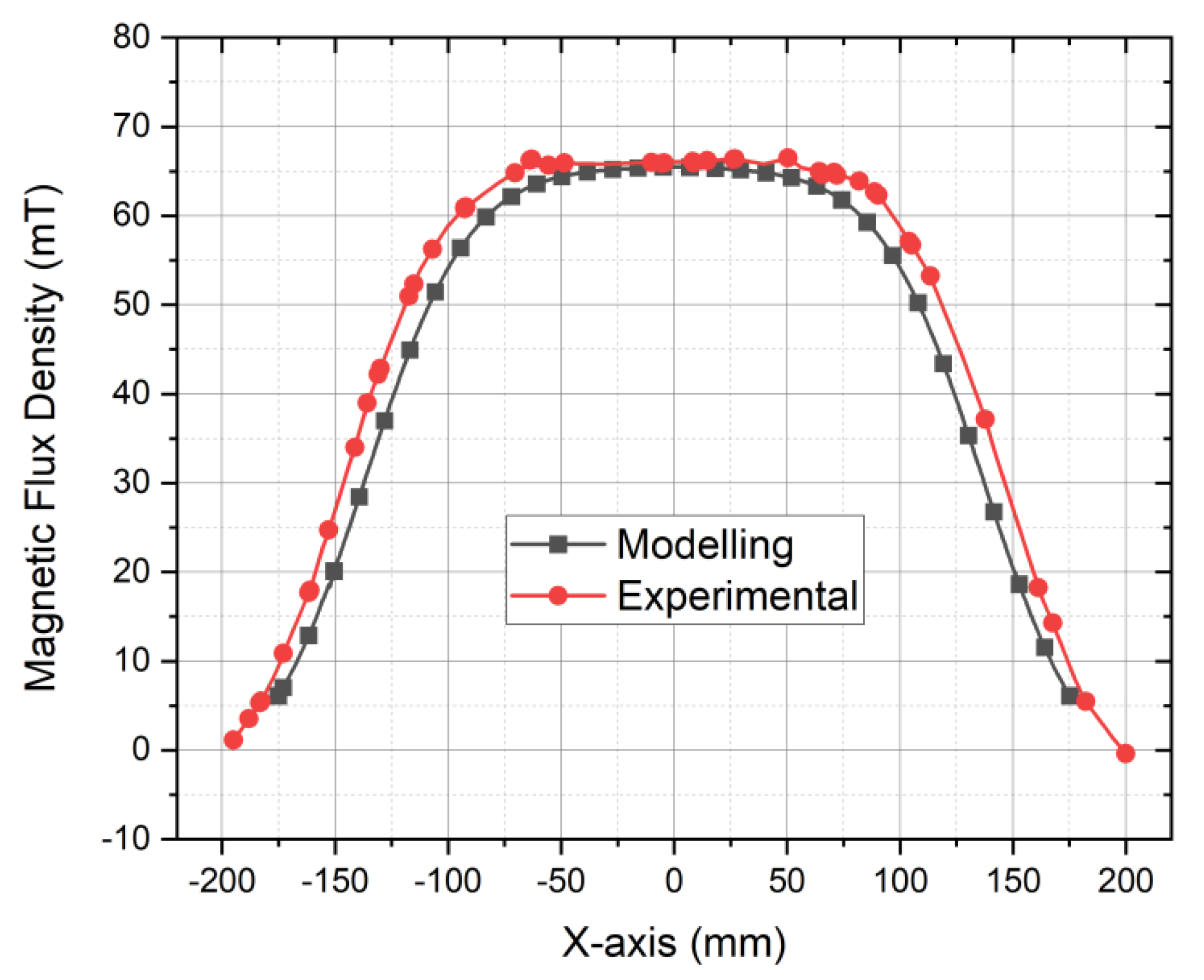
2.5. Experiment vs. Modelling

To verify the FEM model built in this paper, an experimental HTS magnet is fabricated and tested. Figure 6 shows a comparison of the modelling and experimental data. The magnet is scaled down to about a third of the size of the magnet designed above. The experimental magnetic field data (Bz) is obtained by scanning the Hall probe along the central line 60 mm above the magnet.
As shown in Figure 6, the experimental and modelling field data agree well in the central area (about 65 mT). In the edging area of the magnet, a negligible difference of around 5 mT appears because the current distribution inside the superconducting tapes is regarded as homogenous in the simulation for simplification, which should be highly inhomogeneous in practice. Figure 6 indicates that the FEM model built in this paper is capable of predicting the field performance of the HTS magnets with a good accuracy.

3. In-Depth Physical Phenomenon of HTS Magnet

3.1. Electric Current Distribution of the HTS Magnet

Performing an in-depth study on the physical phenomenon of the HTS magnet is beneficial to understand and design the high-speed maglev based on the superconducting technology. As the in-depth mechanism of a superconductor is different from that of normal metal conductors, we established a more advanced model for the professional superconducting modelling based on the H-formulation FEM platform [20]. Our previous study also shows a delicate flowchart of the working principle of H-formulation [21]. The governing equation is:
( μ 0 μ r H ) t + × ( ρ × H ) = 0
where H is the magnetic field intensity, µ0 is the vacuum permeability, and µr is the relative permeability of the material. The detailed derivations of different forms of H-formulation and the ways to import constant/variable permeabilities can be found in our previous study [22]. By using this model, the detailed physical phenomenon of the HTS magnet can be seen and analysed (e.g., the electric current density and superconducting AC loss).
An important physical behaviour in which the superconductor is different from conventional metal conductors is that the electric current density distribution is non-uniform over the cross-section. If we look at the cross-section of the straight part of the racetrack HTS magnet, by taking advantage of symmetry characteristics, we only need to simulate the upper three HTS stacks (one-fourth of the whole cross-section, 3 out of 12). Here the homogenisation method was used to simulate hundreds of turns of the HTS magnet. The homogenisation method can efficiently reduce the computation time but still have good accuracy of superconducting modelling. Details and examples of the homogenisation method can be found in [23,24]. Figure 7 shows the electric current density distribution of the upper three HTS stacks, with the transport currents of (a) 200 A, (b) 400 A, (c) 600 A, and (d) 800 A. It can be discovered that with the transport current increasing from 200 to 600 A, the current occupying area of all the three stacks was increasing. With a transport current of 800 A, the uppermost HTS stack almost occupied the entire cross-section. It is understandable that each HTS stack should transport the same current in total, but the uppermost HTS stack occupied much more area of the current density, as there were both “+” and “−” currents over the cross-section due to the effect of the superconducting magnetisation current. This physical phenomenon of the superconductor was fairly difficult to be noticed by the experiment, but is useful for analysing the HTS magnet for maglevs.

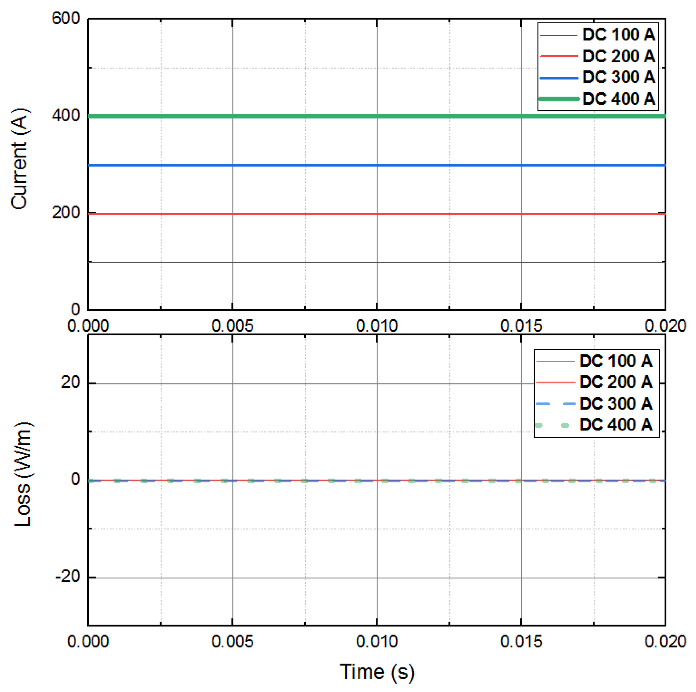
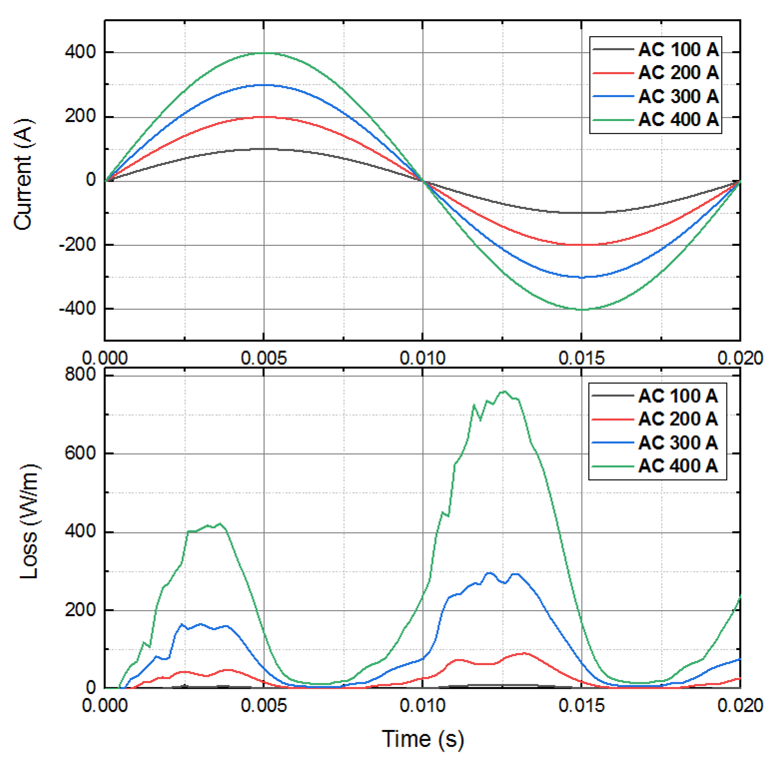
3.2. Loss in the HTS Magnet

Superconducting wires are generally regarded as the perfect conductors, which have the zero-loss characteristics. However, the zero-loss status of superconductors only exists with the direct current (DC) or in the presence of a static magnetic field. Superconducting wires suffer a certain amount of loss when they are involved in the alternating current (AC) system (e.g., with the AC transport current or AC magnetic field). The AC loss from the superconducting wires will be converted to heat energy. Therefore, calculating the AC loss of the HTS magnet in the maglev is important as it may affect the cryogenic system. Fortunately, according to our previous studies, the AC loss can be accurately computed by the H-formulation [22,25].
When the superconducting maglev is operating in the steady-state (e.g., constant speed running), the current in the HTS magnet is DC. As long as the DC current is below the critical current, the HTS magnet does not have any loss. Figure 8 shows the HTS magnet with DC currents of 100, 200, 300, and 400 A, and it can be seen that with all these DC currents the losses of the HTS magnet are always 0.
When the superconducting maglev is operating in the altering-state (e.g., starting up with a ramping current), the current in the HTS magnet is no longer DC. If the current is changing, the issue will be classified as the AC loss problem, and there will be a certain amount of loss in the HTS magnet. For example, Figure 9 presents the losses in the HTS magnet with pure 50 Hz AC sinusoidal currents of 100, 200, 300, and 400 A. It can be seen that the losses increase with the increasing AC current non-linearly, but with an exponential factor of about 3–4. The loss reaches approximately 750 W/m with an AC current of 400 A, which would be a significant value if multiplied by the total length of HTS wires. Corresponding to Figure 9, Figure 10 uses the professional superconducting AC loss unit Joule/cycle/m, with the log-log axis, to assess the loss values. It has the advantage of removing the frequency dependence. The loss curve is about four orders higher than the average of the Norris strip and Norris ellipse [26]. Despite the fact that these cases of the pure AC sinusoidal current seldom happen in the real Maglev operation, these data are still helpful to give the upper limits of some worst high-loss cases.
When the superconducting maglev suffers some instability (e.g., fluctuations of the power supply), the transport current in the HTS magnet is not pure DC but with some small AC components (e.g., ripples). Figure 11 shows the losses in the HTS magnet with a 360 A DC current and 50 Hz AC sinusoidal ripple currents of 10, 30, and 50 A. From 0 s to 0.1 s, before the ripples start, the loss is 0 as expected for all the cases. From 0.1 s to 0.2 s, five cycles of sinusoidal ripples correspond to five peaks of loss curves, and the first ripple losses reach the peak loss points and then attenuate. For the 50 A ripple cases, the peak loss reaches approximately 70 W/m. It can be seen that the ripple currents can also cause a considerable amount of losses. This kind of instability AC loss will result in the form of heat dissipation, and the Maglev cryogenic system should cope with this level of loss in a short time. The constant ripple cases still seldom happen in the maglev, but compared with the pure AC sinusoidal current cases, the ripple cases are closer to the real operation of superconducting maglev with possible harmonics and instability of power supply.
The sinusoidal AC loss, ripple AC loss, and other types of AC losses can be straightaway converted to the heat dissipation, which leads to burdens and problems for the cryogenic system. If these AC losses exceed a certain threshold, the accumulated heat would cause the initiation and propagation of a quench in the superconducting magnet, leading to the loss of magnetic levitation. This issue is extremely important and could be carefully analysed in a future work.

4. Conclusions

This article presents a fundamental study on the design and modelling of the superconducting magnet for the high-speed maglev, which includes the aspects of mechanics, electromagnetics, and loss analysis during instability. The superconducting wire measurements of the critical current in the presence of different magnetic fields with different temperatures were performed. The basic configuration of the HTS magnet (pair) was designed and modelled, and the operating current was set to 350–360 A at a temperature of 20 K, which could meet the electromagnetic requirements of the magnetic field and force. The modelling design of the HTS magnet was verified by a scaled experimental HTS magnet, whose agreement of central magnetic fields has proved that the model is able to well predict the field performance of the HTS maglev magnets. A professional FEM model using the H-formulation was built to investigate the physical phenomenon of the HTS magnet, such as the current density and the loss in the HTS magnet particularly when the maglev is encountering instability. These results could be beneficial for the analysis of the stability and safety of the HTS maglev.

Author Contributions

Conceptualisation, J.J. and B.S.; methodology, B.S., J.J., and L.H.; software, Z.W. and B.S.; validation, Z.W., L.H., and J.J.; formal analysis, Z.W., L.H., and B.S.; investigation, Z.W., B.S., and J.Z.; writing—original draft preparation, B.S., Z.W., J.J., and L.H.; writing—review and editing, J.Z., Y.G., and J.J.; supervision, J.J. and B.S. All authors have read and agreed to the published version of the manuscript.

Funding

This research received no external funding.

Institutional Review Board Statement

Not applicable.

Informed Consent Statement

Not applicable.

Data Availability Statement

The data presented in this study are available on request from the corresponding author.

Acknowledgments

The authors thank Shanghai Superconductor Technology Co. Ltd., for the measurement of the critical current of the superconducting wire.

Conflicts of Interest

The authors declare no conflict of interest.

References

  1. Mohajan, H. The first industrial revolution: Creation of a new global human era. J. Soc. Sci. Humanit. 2019, 5, 377–387. [Google Scholar]
  2. Liu, Z.; Long, Z.; Li, X. Maglev train overview. In Maglev Trains; Springer: Berlin/Heidelberg, Germany, 2015; pp. 1–28. [Google Scholar]
  3. Powell, J.; Danby, G. A 300-mph magnetically suspended train. Mech. Eng. 1967, 89, 30. [Google Scholar]
  4. Sawada, K. Outlook of the superconducting maglev. Proc. IEEE 2009, 97, 1881–1885. [Google Scholar] [CrossRef]
  5. Jin, J.X.; Sheng, G.; Bi, Y.F.; Song, Y.T.; Liu, X.L.; Chen, X.; Li, Q.; Deng, Z.G.; Zhang, W.H.; Zheng, J.; et al. Applied Superconductivity and Electromagnetic Devices - Principles and Current Exploration Highlights. IEEE Trans. Appl. Supercond. 2021, 31, 7000529. [Google Scholar] [CrossRef]
  6. Wang, J.; Wang, S.; Zeng, Y.; Huang, H.; Luo, F.; Xu, Z.; Tang, Q.; Lin, G.; Zhang, C.; Ren, Z. The first man-loading high temperature superconducting maglev test vehicle in the world. Phys. C Supercond. 2002, 378, 809–814. [Google Scholar] [CrossRef]
  7. Kovalev, K.; Koneev, S.; Poltavec, V.; Gawalek, W. Magnetically levitated high-speed carriages on the basis of bulk HTS elements. In Proceedings of the 8th Internerational Symposium Suspension Technology Technology (ISMST’8), Stanford, CA, USA, 15–17 August 2005; p. 51. [Google Scholar]
  8. Okano, M.; Iwamoto, T.; Furuse, M.; Fuchino, S.; Ishii, I. Running performance of a pinning-type superconducting magnetic levitation guide. J. Phys. Conf. Ser. 2006, 43, 244. [Google Scholar] [CrossRef]
  9. Schultz, L.; de Haas, O.; Verges, P.; Beyer, C.; Rohlig, S.; Olsen, H.; Kuhn, L.; Berger, D.; Noteboom, U.; Funk, U. Superconductively levitated transport system-the supratrans project. IEEE Trans. Appl. Supercond. 2005, 15, 2301–2305. [Google Scholar] [CrossRef]
  10. D’ovidio, G.; Crisi, F.; Lanzara, G. A “v” shaped superconducting levitation module for lift and guidance of a magnetic transportation system. Phys. C Supercond. 2008, 468, 1036–1040. [Google Scholar] [CrossRef]
  11. Deng, Z.; Zhang, W.; Zheng, J.; Wang, B.; Ren, Y.; Zheng, X.; Zhang, J. A high-temperature superconducting maglev-evacuated tube transport (hts maglev-ett) test system. IEEE Trans. Appl. Supercond. 2017, 27, 3602008. [Google Scholar] [CrossRef]
  12. Mattos, L.; Rodriguez, E.; Costa, F.; Sotelo, G.; De Andrade, R.; Stephan, R. Maglev-cobra operational tests. IEEE Trans. Appl. Supercond. 2016, 26, 3600704. [Google Scholar] [CrossRef]
  13. Kuwano, K.; Igarashi, M.; Kusada, S.; Nemoto, K.; Okutomi, T.; Hirano, S.; Tominaga, T.; Terai, M.; Kuriyama, T.; Tasaki, K. The running tests of the superconducting maglev using the hts magnet. IEEE Trans. Appl. Supercond. 2007, 17, 2125–2128. [Google Scholar] [CrossRef]
  14. Kusada, S.; Igarashi, M.; Nemoto, K.; Okutomi, T.; Hirano, S.; Kuwano, K.; Tominaga, T.; Terai, M.; Kuriyama, T.; Tasaki, K. The project overview of theHTS magnet for superconducting maglev. IEEE Trans. Appl. Supercond. 2007, 17, 2111–2116. [Google Scholar] [CrossRef]
  15. Terai, M.; Igarashi, M.; Kusada, S.; Nemoto, K.; Kuriyama, T.; Hanai, S.; Yamashita, T.; Nakao, H. The R&D project of HTS magnets for the superconducting maglev. IEEE Trans. Appl. Supercond. 2006, 16, 1124–1129. [Google Scholar]
  16. Zheng, J.; Huang, H.; Zhang, S.; Deng, Z. A general method to simulate the electromagnetic characteristics of HTS maglev systems by finite element software. IEEE Trans. Appl. Supercond. 2018, 28, 1–8. [Google Scholar] [CrossRef]
  17. Jin, J.X.; Zheng, L.H. Driving models of high temperature superconducting linear synchronous motors and characteristic analysis. Supercond. Sci. Technol. 2011, 24, 55011. [Google Scholar] [CrossRef]
  18. Jin, J.X.; Zheng, L.H.; Guo, Y.G.; Zhu, J.G.; Grantham, C.; Sorrell, C.C.; Xu, W. High-temperature superconducting linear synchronous motors integrated with HTS magnetic levitation components. IEEE Trans. Appl. Supercond. 2012, 22, 5202617. [Google Scholar]
  19. Cai, Y.; Ma, G.; Wang, Y.; Gong, T.; Liu, K.; Yao, C.; Yang, W.; Zeng, J. Semianalytical calculation of superconducting electrodynamic suspension train using figure-eight-shaped ground coil. IEEE Trans. Appl. Supercond. 2020, 30, 3602509. [Google Scholar] [CrossRef]
  20. Shen, B.; Grilli, F.; Coombs, T. Overview of h-formulation: A versatile tool for modelling electromagnetics in high-temperature superconductor applications. IEEE Access 2020, 8, 100403–100414. [Google Scholar] [CrossRef]
  21. Jin, J.X.; Zhang, R.T.; Lin, Z.W.; Guo, Y.G.; Zhu, J.G.; Chen, X.Y.; Shen, B.Y. Modelling analysis of periodically arranged high-temperature superconducting tapes. Phys. C Supercond. 2020, 578, 1353747. [Google Scholar] [CrossRef]
  22. Shen, B.; Grilli, F.; Coombs, T. Review of the AC loss computation for HTS using H formulation. Supercond. Sci. Technol. 2020, 33, 33002. [Google Scholar] [CrossRef] [Green Version]
  23. Zermeno, V.M.; Abrahamsen, A.B.; Mijatovic, N.; Jensen, B.B.; Sørensen, M.P. Calculation of alternating current losses in stacks and coils made of second generation high temperature superconducting tapes for large scale applications. J. Appl. Phys. 2013, 114, 173901. [Google Scholar] [CrossRef] [Green Version]
  24. Wang, Z.; Tang, Y.; Ren, L.; Li, J.; Xu, Y.; Liao, Y.; Deng, X. AC loss analysis of a hybrid HTS magnet for smes based on H-formulation. IEEE Trans. Appl. Supercond. 2016, 27, 4701005. [Google Scholar]
  25. Shen, B.; Li, C.; Geng, J.; Zhang, X.; Gawith, J.; Ma, J.; Liu, Y.; Grilli, F.; Coombs, T.A. Power dissipation in HTS coated conductor coils under the simultaneous action of ac and dc currents and fields. Supercond. Sci. Technol. 2018, 31, 075005. [Google Scholar] [CrossRef]
  26. Norris, W. Calculation of hysteresis losses in hard superconductors carrying ac: Isolated conductors and edges of thin sheets. J. Phys. D Appl. Phys. 1970, 3, 489–507. [Google Scholar] [CrossRef]
Figure 1. High-speed maglev for a proposed top speed over 600 km/h (conceptual design), the HTS magnet, and the magnetic fields.
Machines 10 00113 g001
Figure 2. Working principle of the superconducting electrodynamic suspension of the HTS maglev: (a) HTS magnet and 8-shape coil, (b) equivalent circuit.
Machines 10 00113 g002
Figure 3. The load line of the HTS magnet for maglev and the critical current (Ic) measurements of the HTS wire in different magnetic fields and operating temperatures in order to select the proper operating current of the HTS magnet for maglev.
Machines 10 00113 g003
Figure 4. (a) Magnetic field (T) in the x-direction; (b) magnetic field (T) in the y-direction, (c) magnetic field (T) in the z-direction, (d) force per volume (N/m3 × 108) in the x-direction, (e) force per volume (N/m3 × 108) in the y-direction, and (f) force per volume (N/m3 × 108) in the z-direction on the top surface of the HTS magnet with an operating current of 350 A.
Machines 10 00113 g004
Figure 5. Magnetic flux density in the z-direction (Bz) along the reference lines at 50, 100, and 150 mm above the HTS magnets with an operating current of 350 A.
Machines 10 00113 g005
Figure 6. Experimental and modelling magnetic field of the magnet with the magnetic field (Bz) 60 mm above the magnet.
Machines 10 00113 g006
Figure 7. Electric current density distribution of the upper 3 HTS stacks with transport currents of (a) 200, (b) 400, (c) 600, and (d) 800 A.
Machines 10 00113 g007aMachines 10 00113 g007b
Figure 8. Losses in the HTS magnet with DC currents of 100, 200, 300, and 400 A.
Machines 10 00113 g008
Figure 9. Losses in the HTS magnet with pure 50 Hz AC sinusoidal currents of 100, 200, 300, and 400 A (peak).
Machines 10 00113 g009
Figure 10. Corresponding to Figure 9, losses in the HTS magnet with pure 50 Hz AC sinusoidal currents of 100, 200, 300, and 400 A (peak) converted into the unit of Joule/cycle/m.
Machines 10 00113 g010
Figure 11. Losses in the HTS magnet with a 360 A DC current and 50 Hz AC sinusoidal ripple currents of 10, 30, and 50 A (peak).
Machines 10 00113 g011
Table 1. Parameters of the HTS magnet for the maglev.
ComponentsSpecifications
Coil shapeRacetrack
Coil typeDouble-pancake (DP)
Turns2 × 500
Number of DPs for each HTS magnet3
Size of each HTS magnet1050 mm × 510 mm × 72 mm
Operating current350–360 A
Operation temperature20 K
Publisher’s Note: MDPI stays neutral with regard to jurisdictional claims in published maps and institutional affiliations.

