Stiffness-Performance-Based Redundant Motion Planning of a Hybrid Machining Robot

Abstract

Large-scale components usually have complex structures with high local stiffness, and the holes on them are required to be machined with high precision, which makes it important and challenging to study how to efficiently and precisely drill in the large-scale components. This article presents mobile hybrid machining equipment that consists of a five-axis parallel module, a 2-degree-of-freedom (DoF) robotic, arm and an automated guide vehicle (AGV) connected in series. With the ability of wide-range positioning and precise local processing, it has potential advantages in the drilling processing of large-scale components. Stiffness is one of the most important performances for machining equipment, and it’s highly related to the its configuration. For the discussed equipment, the stiffness is determined by the two-stage-positioning hybrid machining robot, which comprises a five-axis parallel module and a two-DoF robotic arm. The redundant motion of the hybrid machining robot makes it possible to optimize its configuration by reasonably planning redundant motion. Therefore, a redundant motion-planning method based on stiffness performance is proposed. A kinematic analysis of the five-axis parallel module, the robotic arm, and the hybrid machining robot is carried out. A hybrid robot usually consists of several subsystems, and to take the compliance of each subsystem into consideration, the stiffness-modeling method for the hybrid robot with n subsystems connected in series is proposed. The stiffness model of the hybrid machining robot is established by using this method, and the variation of the stiffness magnitude has the same trend as that obtained by using FEA software. Stiffness magnitude and isotropy indices are proposed to evaluate the robot’s stiffness performance along the axis of the spindle and in the plane perpendicular to the axis of the spindle. The redundant motion of the hybrid machining robot is planned by maximizing the stiffness magnitude along the spindle axis, with priority to the stiffness isotropy index. Finally, the drilling experiment is carried out, and the results show that the relative error of the hole diameter obtained under the optimal configuration of the hybrid machining robot is 1.63%, which is smaller than those obtained under the other two configurations for comparison with relative errors of 3.75% and 3.50%, respectively. It proves the validity of the redundant motion-planning method. The proposed stiffness-modeling method and the stiffness-performance indices are also applicable to other hybrid machining robots.

1. Introduction

With rapid development in the fields of aerospace, transportation, energy, and shipping, there is an increasingly urgent demand for processing large-scale components such as spacecraft cabins, high-speed train bodies, and pressure vessels. These components usually have a complex structure, have a large size, and come with high local stiffness, and the holes on them have drilling demands that require high precision. At present, there are three main methods for drilling holes in large-scale components: (1) using large processing machine tools [1] when their strokes are sufficient for the task in hand, which is the typical representative of inclusive processing mode, and this will cost a lot in designing and manufacturing, and the processing flexibility is hard to meet the diversified processing needs of large-scale components [2]; (2) manually processing [3], which requires high technical skills and long working hours for working staff, and it is inefficient and cannot guarantee product quality and consistency; (3) using a mobile machining robot system, which has the advantages of high flexibility, good accessibility, and motion dexterity [4]. It makes up for the shortage of large machine tools and provides a new idea to solve the problem of efficiently and precisely drilling in large-scale components [5].

Given the advantages of mobile robots, serial robotic arms, which have a large workspace and especially high dexterity, have been used in drilling holes in large-scale components [6,7]. However, serial robots are limited in high-precision machining because of their relatively low stiffness [4,7] and large variation of stiffness in the workspace. As a counterpart to serial robotic arms, parallel robots usually have a compact structure, high stiffness, and the ability to support heavy load and work with good precision [8], such as the five-axis parallel robots developed by Metrom [9], Tricept, and TriVariant [10]. Combining the advantages of the robotic arm and parallel robot, a type of mobile hybrid machining equipment [11] is designed, which consists of an AGV (Automated Guide Vehicle), a two-DoF (Degree-of-Freedom) robotic arm, and a five-axis parallel module connected in series. It has a large workspace (up to 1.7 m in vertical direction) and local fine machining capability, which makes it suitable for drilling in large-scale components. For this robot, its machining accuracy is mainly decided by the two-stage-positioning hybrid machining robot, which comprises a five-axis parallel module and a two-DoF robotic arm. For improving the machining accuracy of a robot, robust design [12], high-precision calibration, and configuration optimization are common methods. The robust design is usually used at the design stage to make the robot insensitive to geometric tolerance, calibration can improve its positioning accuracy, and configuration optimization can improve its stiffness performance. The five-axis parallel module and the robotic arm have overlapping DoFs in two translational directions, which makes it possible to improve the robot’s machining performance by reasonably planning the redundant motion.

Stiffness has a great influence on machining performance. For a particular robot, its stiffness can be improved only by changing the robot’s configuration [13]. Therefore, it is necessary to study the variation of robot stiffness with configuration. At present, there are three main methods in this area, namely finite element analysis (FEA), matrix structural analysis (MSA) and virtual joint modeling (VJM). The FEA is a relatively accurate method, and it is usually used at the final design stage because of its time-consuming routine [14,15]. Based on the basic idea of the FEA, the MSA was proposed. Deblaise et al. [11] used the MSA to establish the stiffness model of Delta. It improves the efficiency of calculation at the cost of accuracy [16,17,18], and it is generally applicable to systems composed of rods because the elements are generally considered to have regular shapes [19]. Different from the FEA and MSA, Gosselin [20] took the constraint compliance into consideration and proposed a method based on the VJM, and it is widely applied in stiffness modeling for fully parallel robots [16,21,22]. Cao et al. [23] established the stiffness model of an overconstrained parallel robot by analyzing the strain energy of each limb by using the structural decomposition strategy. These studies focused mainly on a single parallel robot. As for a hybrid robot comprising several subsystems, it is important to consider the impact of every subsystem’s stiffness on the stiffness of the hybrid robot. Chen et al. [24] considered the base as the front-end subsystem and established the stiffness model of an adsorption machining robot by factoring in the stiffness of the base. Because the coordinate origins of the base and the adsorption machining robot were the same, the mapping relationship between the stiffness of the base and the stiffness of the adsorption machining robot wasn’t described in detail, which has an impact on the stiffness of the hybrid robot when the coordinate origin of each subsystem is different.

Planning the redundant motion usually means optimizing the kinematic and stiffness performance of the robot under certain restrictions. Constraints like singularity, collision, and power consumption for redundant manipulators were proposed in [25,26,27], and the joint trajectories were planned well to ensure collision avoidance with relatively low power consumption. Liao et al. [28] proposed a region-based toolpath-generation method, and it can improve the stiffness of the robot in freedom-surface machining. The redundant motion-planning methods mentioned above usually depend on machining process and require adjusting the tool pose in real time, which may reduce machining efficiency. Off-line programming can significantly improve processing quality and efficiency [13], and it usually needs indices to evaluate the stiffness performance of the robot. Jiao et al. [13] proposed a stiffness-performance index in the feed direction for a serial drilling robot, on the basis of which a redundancy resolution was put forward, and it achieved optimum stiffness during the drilling process and was kept away from singularity. In addition to the stiffness in the feed direction, the stiffness isotropy proved to be important for machining robot [13]. Chen et al. [24] proposed a stiffness isotropy index, on the basis of which an evaluation of the stiffness was carried out and an optimized workspace was identified.

Although stiffness modeling for robots has been well studied, further research accounting for the impact of the stiffness of subsystems on that of the hybrid robot is relatively limited. The stiffness evaluation indices for redundant motion planning proposed in the previous studies have clear physical meanings, but the robot configurations obtained by the above indices may not be the optimal drilling configurations. Therefore, the research of redundant motion planning based on stiffness performance is still needed. This article aims to propose a stiffness-modeling method for hybrid robots while accounting for the impact of the stiffness of each subsystem, and it proposes a stiffness index in the plane perpendicular to the tool axis while taking into account the magnitude and isotropy at the same time. Based on the stiffness index, the redundant motion of the hybrid machining robot will be planned and the optimal configuration will be used to carry out the drilling processing on the large-scale components.

Taking a seven-DoF hybrid machining robot as the study subject, this article establishes the stiffness model and proposes stiffness-performance indices, on the basis of which the redundant motion of the hybrid machining robot is planned and the optimal configuration for drilling is obtained. The remainder of the article is organized as follows: In Section 2, the configuration of the hybrid machining robot is introduced in detail, and the kinematic models of the five-axis parallel module, the robotic arm, and the hybrid machining robot are established step by step. In Section 3, a stiffness-modeling method for a hybrid robot with n subsystems connected in series is proposed; the stiffness model of the hybrid machining robot is established using this method; and the variation of the stiffness magnitude has the same trend as that obtained by the FEA software. In Section 4, the stiffness magnitude and isotropy indices are proposed. Stiffness evaluation and redundant motion planning are carried out by using the indices as a base. A drilling experiment is carried out in Section 5, and it proves the validity of the redundant motion-planning method. In Section 6, the article is concluded.

2. Kinematic Modeling of the Hybrid Machining Robot

The stiffness of a robot is highly related to its configuration, so it is important to study how the stiffness performance of the robot varies with its configuration. The stiffness-performance analysis is on the basis of kinematic analysis. As described in Section 1, the hybrid machining robot is a two-stage-positioning robot that consists of a five-axis parallel module and a two-DoF robotic arm connected in series. In this section, these two subsystems are introduced in detail, and the kinematic modeling of the five-axis parallel module, the robotic arm, and the hybrid machining robot is sequentially carried out.

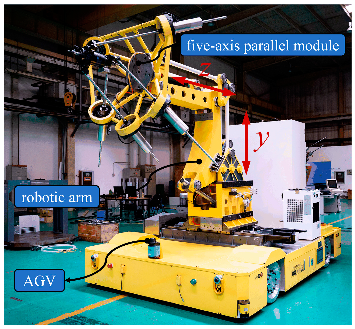
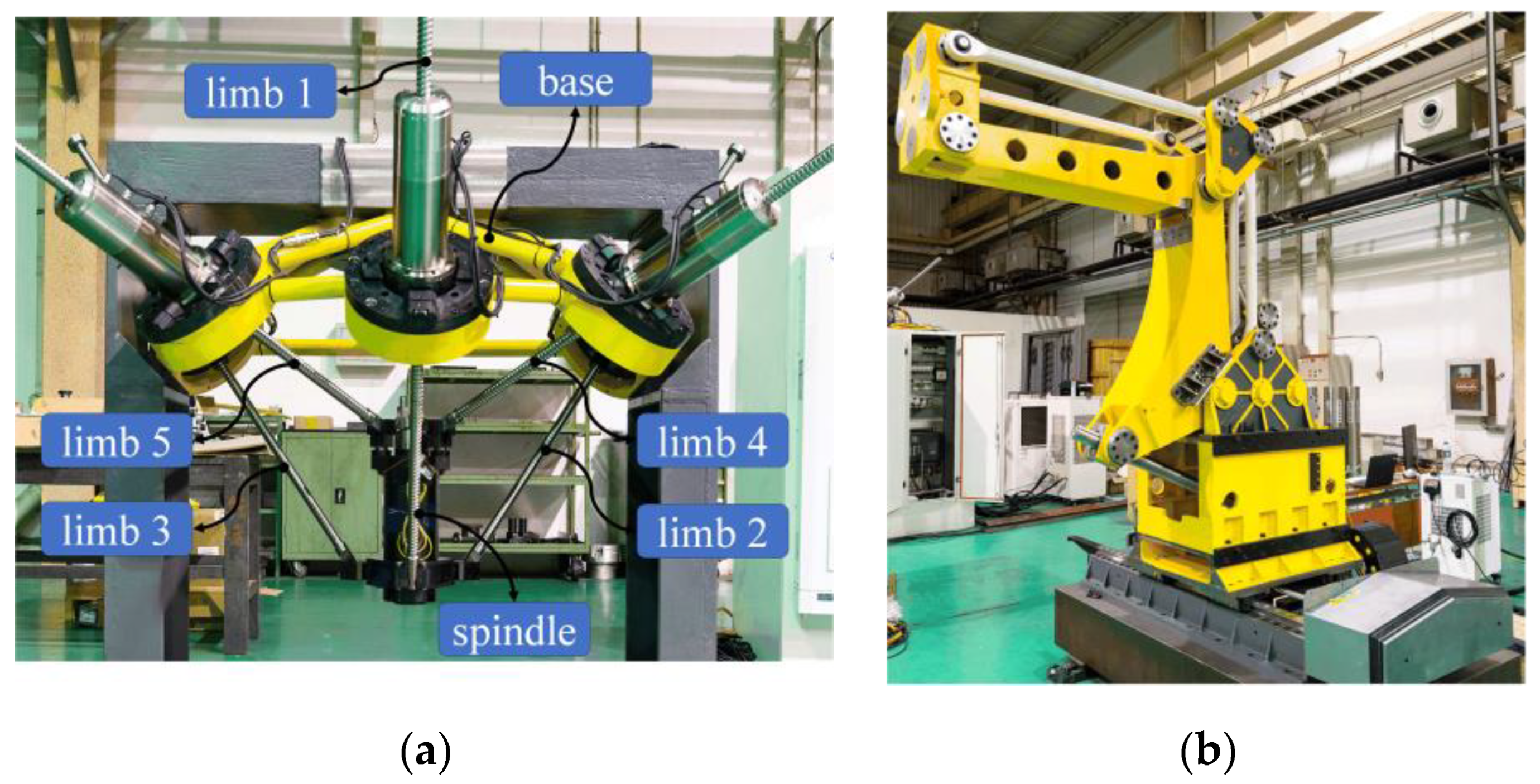
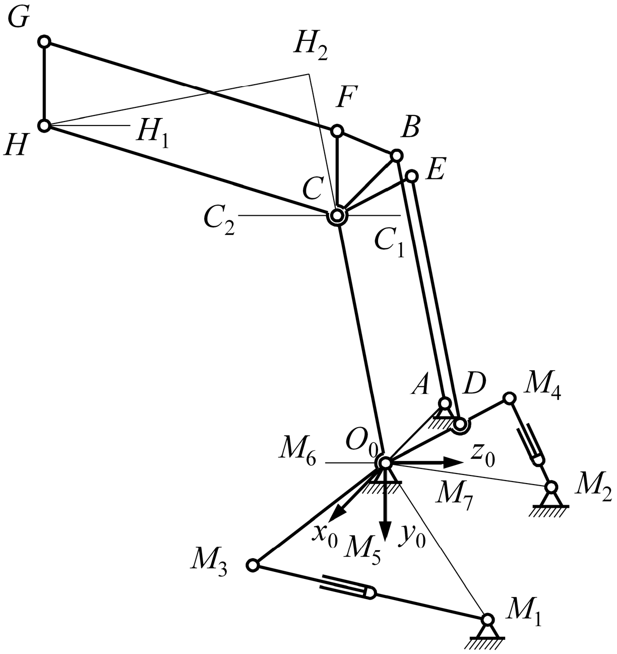
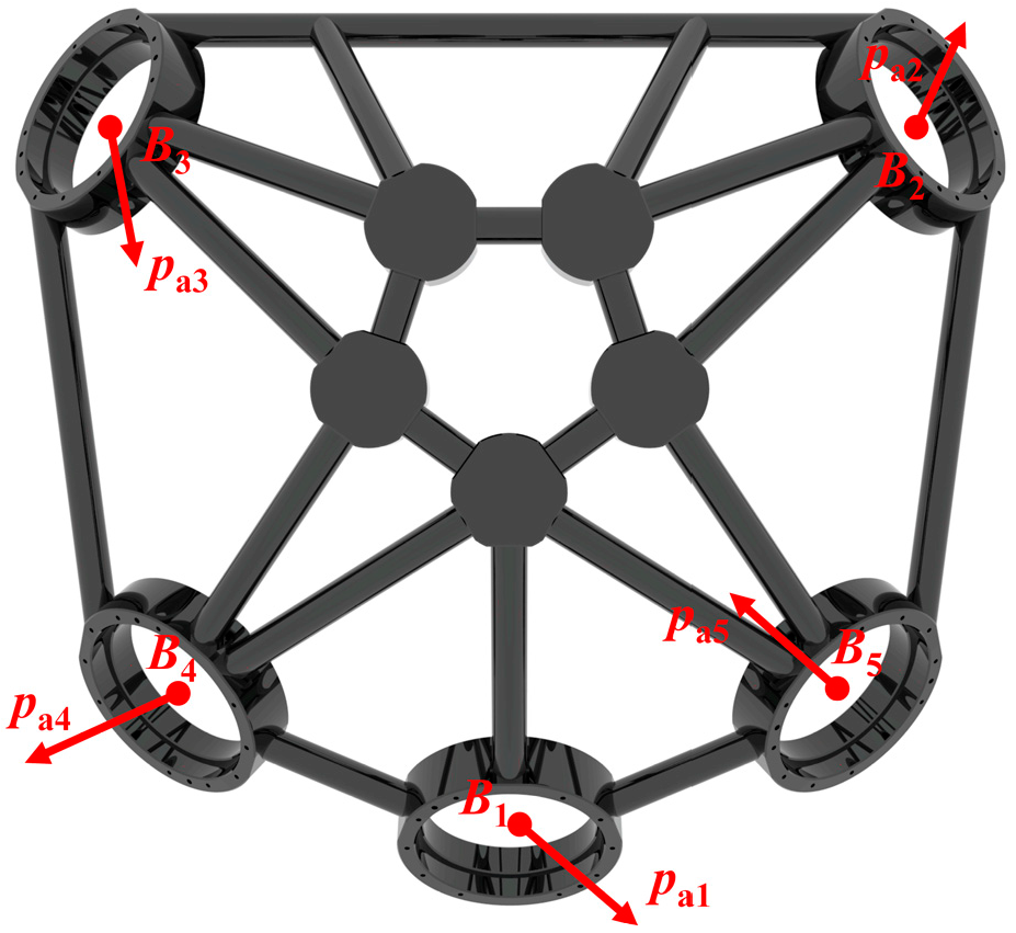
2.1. Introduction to the Hybrid Machining Robot

The hybrid machining equipment is shown in Figure 1. It consists of an AGV, a two-DoF robotic arm, and a five-axis parallel module. The two-DoF robotic arm and the five-axis parallel module make up the hybrid machining robot discussed in this article. During processing, the AGV will be stably supported with the ground. Subsequently, the robotic arm moves in a wide range to stably position the five-axis parallel module near the area to be processed. Finally, the actuating joints of the robotic arm are locked, and the five-axis parallel module is used to complete precise local processing.

As shown in Figure 2a, the five-axis parallel module is based on a 4-UCU&UCR spatial mechanism, where limb 1 is a UCR kinematic chain and the other four limbs are UCU kinematic chains. Here U, C, and R represent a Hooke joint, a prismatic joint driven by electric ball screw, and a revolute joint, respectively. The workspace of the five-axis module is a cube with 300 mm × 300 mm × 200 mm and has the ability to rotate at least 20° in an arbitrary direction.

The robotic arm is shown in Figure 2b. It is driven by three prismatic joints and has three translational DoFs. When the guideway is fixed, it degenerates into a two-DoF robotic arm. The plane in which the end moves is defined as the working plane of the robotic arm. There are three parallelograms to ensure that higher stiffness can be guaranteed, and the end is always in vertical attitude when the robotic arm moves. The workspace of the two-DoF robotic arm is shown in Figure 3.

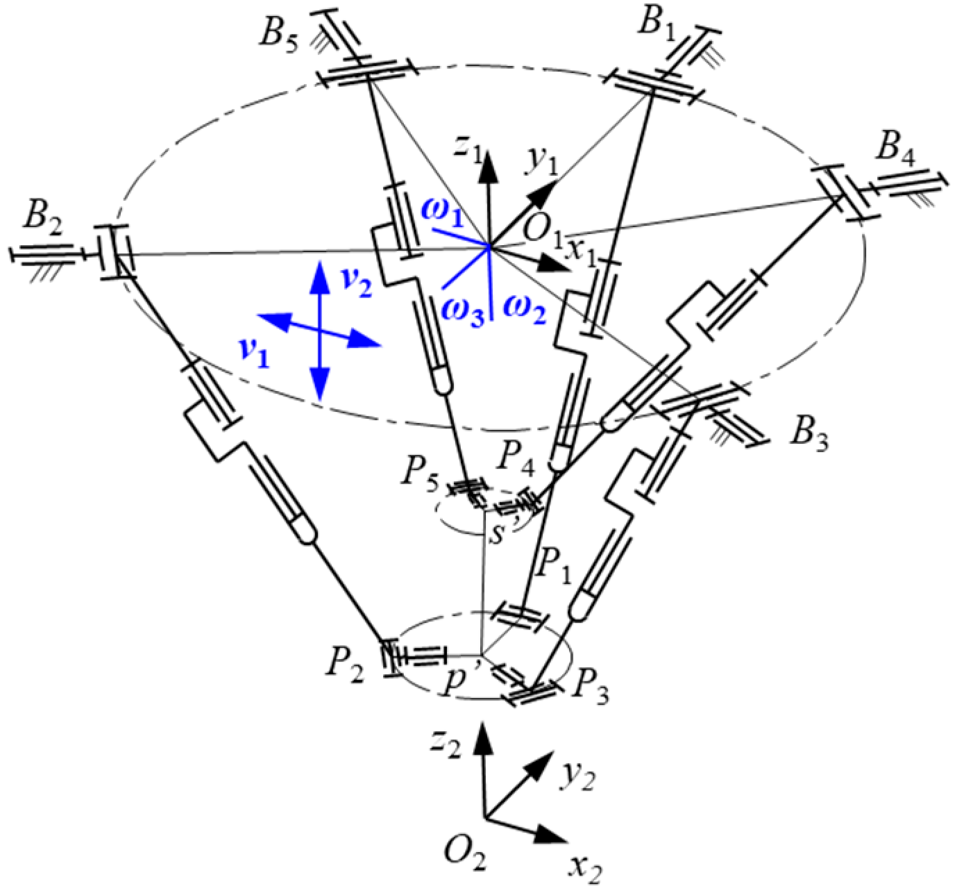
2.2. Kinematic Modeling of the Five-Axis Parallel Module

For this lower mobility mechanism, the traditional Jacobian matrix is obtained by accounting for only the actuation direction of kinematic chains, and its order is usually less than six. Therefore, the stiffness model that is established based on it usually ignores the effect of the constraint compliance. In order to take the constraint compliance into account and obtain the Jacobian matrix with the same order as the stiffness matrix, a kinematic analysis of the parallel mechanism is required, which includes inverse kinematics and deformation analysis in the direction of actuations and constraints.

The inverse kinematics means to solve the configuration of the five-axis parallel module when the position and the orientation of the spindle are fixed. The kinematic scheme of the five-axis parallel module is shown in Figure 4, in which B_i (i = 1~5) represents the center of Hooke joints connected to the base of limb i, P₁ represents the center of revolute joint connected to the spindle of limb 1, and P_i (i = 2~5) represents the center of Hooke joints connected to the spindle of limb 2~5. Points B₁~B₅ are on the same circle. Points P₁~P₅ are located in two layers. Points P₁~P₃ are on the same circle, with point p′ as the center in the lower layer. Points P₄ and P₅ are on the same circle, with point s′ as the center in the upper layer. The base frame, O₁-x₁y₁z₁, is attached to the base, and the origin, O₁, is the center of the circle, where points B₁~B₅ are. The y-axis is collinear to O₁B₁, and the z-axis is perpendicular to the circle plane. The x-axis is decided by the right-hand rule. The spindle frame, O₂-x₂y₂z₂, is attached to the spindle, and the origin, O₂, is the end of the cutter. The y’-axis is collinear to p′P₁, and the z’-axis is collinear to p′s′. The x’-axis is decided by the right-hand rule.

The position and orientation of the spindle in the base coordinate frame, O₁-x₁y₁z₁, can be expressed by ${\left[x_1{,y}_1{,z}_1{,f}_1{,\theta }_1\right]}^{\mathrm{T}}$, where ${\left[x_1{,y}_1{,z}_1\right]}^{\mathrm{T}}$ describes the position of point O₂ in the coordinate frame, O₁-x₁y₁z₁, and ${\left[f_1{,\theta }_1\right]}^{\mathrm{T}}$ describes the azimuth and tilt angles. The key structural parameters are as follows: OB_i = R₁, p′P₁ = R₂, s′P₄ = R₃, s′p′ = H_a, s′O′ = L_c, $\angle { B}_4{\mathit{OB}}_5{=2\alpha }_1$, and $\angle { P}_4{p^{\prime }P}_5{=2\alpha }_2$.

In the base coordinate frame, O₁-x₁y₁z₁, the position of B_i can be described by O₁B_i (i = 1~5). In the spindle coordinate frame, O₂-x₂y₂z₂, the position of P_i can be described by O₂P_i (i = 1~5). The rotation matrix of spindle can be written as

R = [x₂ y₂ z₂]^T

(1)

where z₂ is related only to the magnitude of f₁ and θ₁, so z₂ can be expressed as

z₂ = [cosf₁sinθ₁  sinf₁sinθ₁cosθ₁]^T

(2)

According to the constraint of limb 1, O₂x₂ is perpendicular to plane s′P₁B₁, so x₂ can be expressed as

$${\mathit{x}}_2=\frac{{\mathit{O}}_2{\mathit{B}}_1\times {\mathit{z}}_2}{\left|\right|{\mathit{O}}_2{\mathit{B}}_1\times {\mathit{z}}_2\left|\right|}$$

(3)

And y₂ can be obtained by the right-hand rule:

$${\mathit{y}}_2=\frac{{\mathit{z}}_2\times {\mathit{x}}_2}{\left|\right|{\mathit{z}}_2\times {\mathit{x}}_2\left|\right|}$$

(4)

After Equations (1)–(4) have been combined, in the base coordinate frame, O₁-x₁y₁z₁, O₂P_i can be described as

$${\mathit{O}}_2{\mathit{P}}_i^{{\mathit{O}}_1}=\mathit{R}{\mathit{O}}_2{\mathit{P}}_i^{{\mathit{O}}_2}$$

(5)

The inverse kinematics of the five-axis parallel module can be obtained as follows:

$${\mathit{L}}_i=\left|\right|{\mathit{O}}_1{\mathit{O}}_2+{\mathit{O}}_2{\mathit{P}}_i^{{\mathit{O}}_1}-{\mathit{O}}_1{\mathit{B}}_i\left|\right|, i=1~5$$

(6)

$${\mathit{l}}_i=\frac{{\mathit{O}}_1{\mathit{O}}_2+{\mathit{O}}_2{\mathit{P}}_i^{{\mathit{O}}_1}-{\mathit{O}}_1{\mathit{B}}_i}{\left|\right|{\mathit{O}}_1{\mathit{O}}_2+{\mathit{O}}_2{\mathit{P}}_i^{{\mathit{O}}_1}-{\mathit{O}}_1{\mathit{B}}_i\left|\right|}, i=1~5$$

(7)

In order to obtain the Jacobian matrix with the same order as the stiffness matrix, the mapping relationship between end-effector deformation and limb deformation in the actuation and constraint directions needs to be solved [16], which can be expressed as

$$\Delta \mathit{\rho }={\mathit{J}}^{\prime }{\Delta }_p$$

(8)

where Δρ represents the deformation of actuation and constraint directions of the limbs and Δ_p represents the deformation of the end effector.

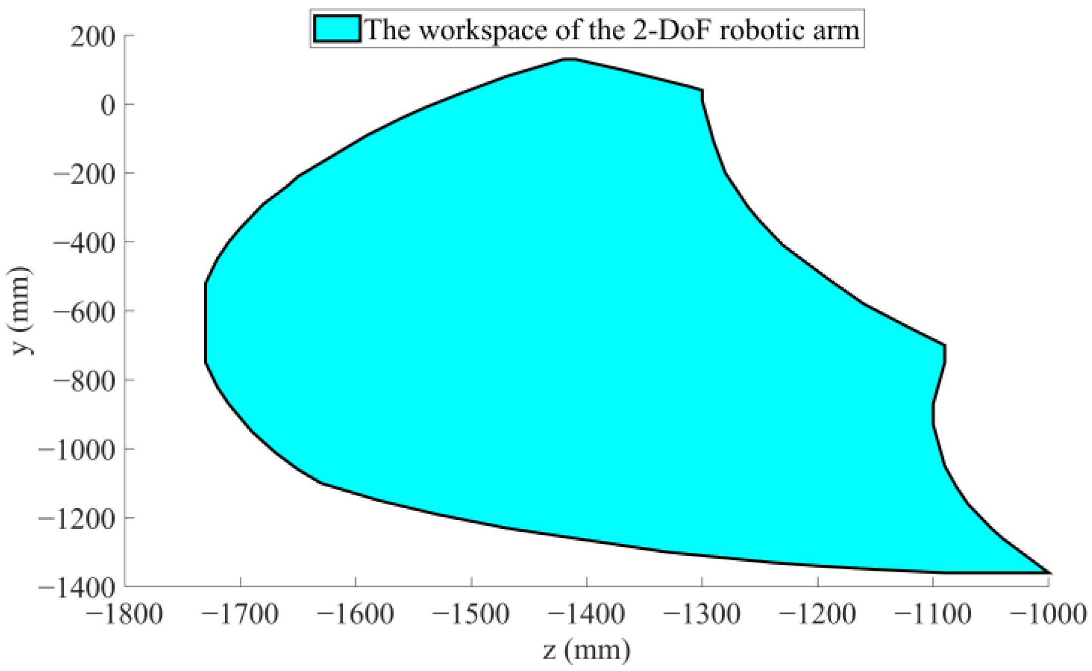
2.3. Kinematic Modeling of the Two-DoF Robotic Arm

To establish the stiffness model of the robotic arm by using the MSA method, the mapping relationship between the pose of each component and the position of the end effector must be studied. Therefore, the inverse kinematics of the robotic arm should be investigated.

The kinematic scheme of the two-DoF robotic arm is shown in Figure 5. The global coordinate frame, O₀-x₀y₀z₀, is attached to the robotic arm, and the origin, O₀, is the center of a fixed revolute joint. The y₀-axis is in the working plane and vertically downward, and the z₀-axis is in the working plane and horizontal to the right. The x₀-axis can be obtained by the right-hand rule. The inverse kinematics of the two-DoF robotic arm can be obtained by plane geometry [21] as

$${|M}_1{M}_3{|}^2{=|\mathit{OM}}_3{|}^2+{|\mathit{OM}}_1{|}^2-2{|\mathit{OM}}_3{\left|\right|\mathit{OM}}_1|\cos \angle M_1{\mathit{OM}}_3$$

(9)

$${|M}_2{M}_4{|}^2{=|\mathit{OM}}_2{|}^2+{|\mathit{OM}}_4{|}^2-2{|\mathit{OM}}_2{\left|\right|\mathit{OM}}_4|\cos \angle M_2{\mathit{OM}}_4$$

(10)

When the lengths of |M₁M₃| and |M₂M₄| are known, the position of each point in the coordinate frame, O₀-x₀y₀z₀, can be calculated. Further, the pose of each component can be obtained. Component AB is an example: the local coordinate frame, O_AB-x′y′z′, and the global coordinate frame, O_AB-x₀y₀z₀, are shown in Figure 6, so the rotation matrix of component AB can be written as

$$\begin{array}{l}{\mathit{\lambda }}_{AB}=\left(\begin{array}{ccc}0& 0& -1\\ -\sin f_{\mathit{AB}}& -\cos f_{\mathit{AB}}& 0\\ -\cos f_{\mathit{AB}}& \sin f_{\mathit{AB}}& 0\end{array}\right)\\ f_{\mathit{AB}}=\mathrm{atan}2(y_C{-y}_H{ , z}_C{-z}_H)\end{array}$$

(11)

where $(y_C,z_C)$ and $(y_H,z_H)$ represent the coordinates of point C and point H, respectively, in coordinate frame O_AB-x₀y₀z₀. The rotation matrices of other components can be obtained in a similar way.

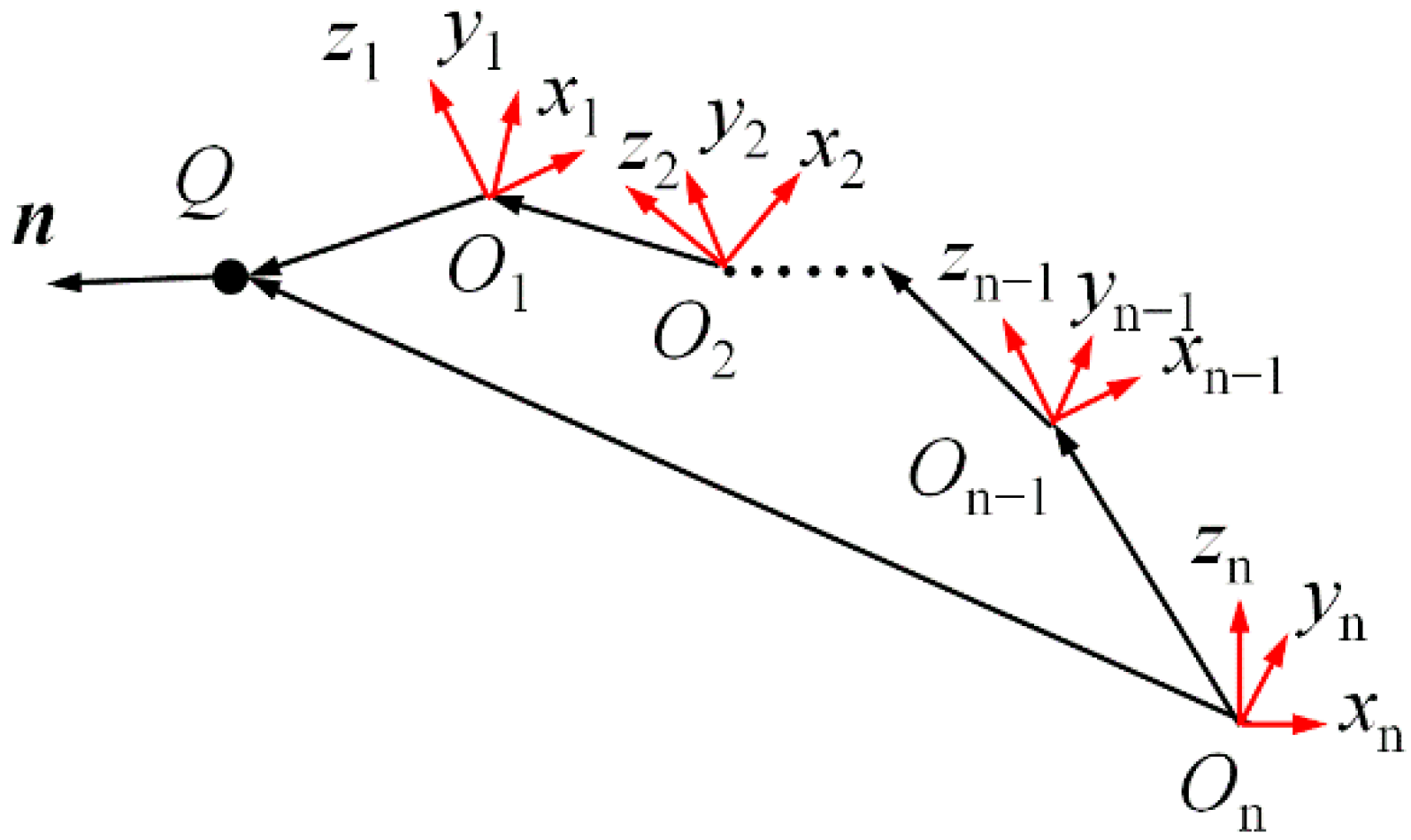
2.4. Kinematic Modeling of the Hybrid Machining Robot

To solve the hybrid machining robot configuration when the spindle’s position and orientation are fixed, conducting a kinematic analysis of the hybrid machining robot is necessary. According to the machining mode mentioned above, the robotic arm should be fixed in a specific position before processing, which can be artificially specified. The length of the two screws can be solved by Equations (9) and (10). The spindle’s position and orientation in the base coordinate frame, O₁-x₁y₁z₁, and the global coordinate frame, O₀-x₀y₀z₀, are shown in Figure 7. In order to solve the length of each limb, the position and orientation of the spindle represented in coordinate frame O₁-x₁y₁z₁ must be obtained. Therefore, the key to specifying the configuration of the hybrid machining robot is to solve the mapping relationship between the spindle’s position and its orientation represented in the global coordinate frame, O₀-x₀y₀z₀, and in the base coordinate frame, O₁-x₁y₁z₁.

In coordinate frame O₀-x₀y₀z₀, the position and orientation of the spindle can be expressed by ${\left[x_0{,y}_0{,z}_0{,f}_0{,\theta }_0\right]}^{\mathrm{T}}$. In coordinate frame O₁-x₁y₁z₁, the position and orientation of the spindle can be expressed by ${\left[x_1{,y}_1{,z}_1{,f}_1{,\theta }_1\right]}^{\mathrm{T}}$. In coordinate frame O₀-x₀y₀z₀, the position of point O₁ can be expressed by ${\mathit{O}}_1^{O_0}$. Thus, the spindle’s position and orientation in coordinate frame O₀-x₀y₀z₀ and in coordinate frame O₁-x₁y₁z₁ can be described as

$$\begin{array}{l}{\mathit{Q}}^{O_0}=(x_0{,y}_0{,z}_0{)}^{\mathrm{T}}\\ {\mathit{n}}^{O_0}=(\cos f_0\sin {\theta }_0 \sin f_0\cos {\theta }_0 \cos {\theta }_0{)}^{\mathrm{T}}\\ {\mathit{Q}}^{O_1}=(x_1{,y}_1{,z}_1{)}^T\\ {\mathit{n}}^{O_1}=(\cos f_1\sin {\theta }_1 \sin f_1\cos {\theta }_1 \cos {\theta }_1{)}^T\end{array}$$

(12)

The rotation matrix of coordinate frame O₁-x₁y₁z₁ is defined as R. The mapping relationship between the spindle’s position and its orientation in the base and global coordinate frames can be expressed as

$$\begin{array}{l}{\mathit{Q}}^{O_0}={\mathit{O}}_1^{O_0}+\mathit{R}{\mathit{Q}}^{O_1}\\ {\mathit{n}}^{O_0}=\mathit{R}{\mathit{n}}^{O_1}\end{array}$$

(13)

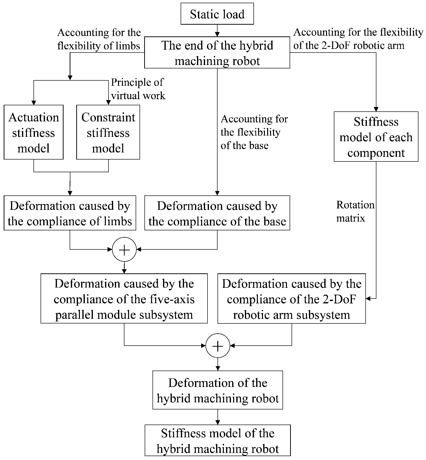
3. Stiffness Modeling

The stiffness performance of a robot is influenced by mainly three factors [13]: (1) the material and structure of the robot; (2) the actuation and constraint systems; and (3) the robot’s configurations. For a given robot, the stiffness performance can be improved only by changing its configuration, so it is necessary to establish the stiffness model of the robot to study how the stiffness performance varies with the robot configuration. The method to establish the stiffness model of the hybrid machining robot is shown in Figure 8. The stiffness model of the five-axis parallel module is established by using the FEA method and the principle of virtual work. The stiffness model of the robotic arm can be obtained by MSA method. The stiffness mapping relationship between the end of the robotic arm and the end of the hybrid machining robot is studied, and the stiffness model of the hybrid machining robot is obtained according to the linear superposition principle.

Because joint friction and bearing deformation have little effect on the end stiffness, they can be ignored when establishing the stiffness model. In addition, the deformation of each component is considered as linear elastic deformation.

3.1. Stiffness Modeling of the Five-Axis Parallel Module

The five-axis parallel module can be divided into the limbs and the base. The VJM and the FEA are used to establish their respective stiffness models as follows.

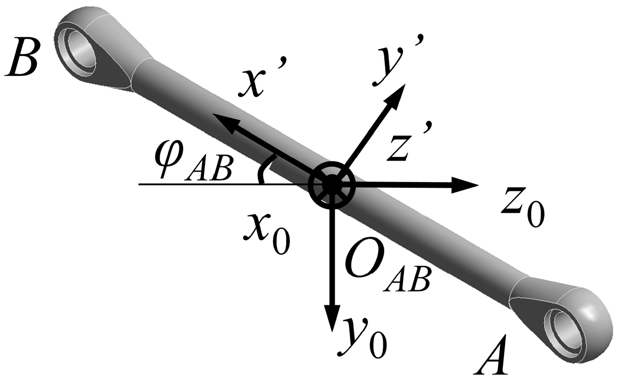
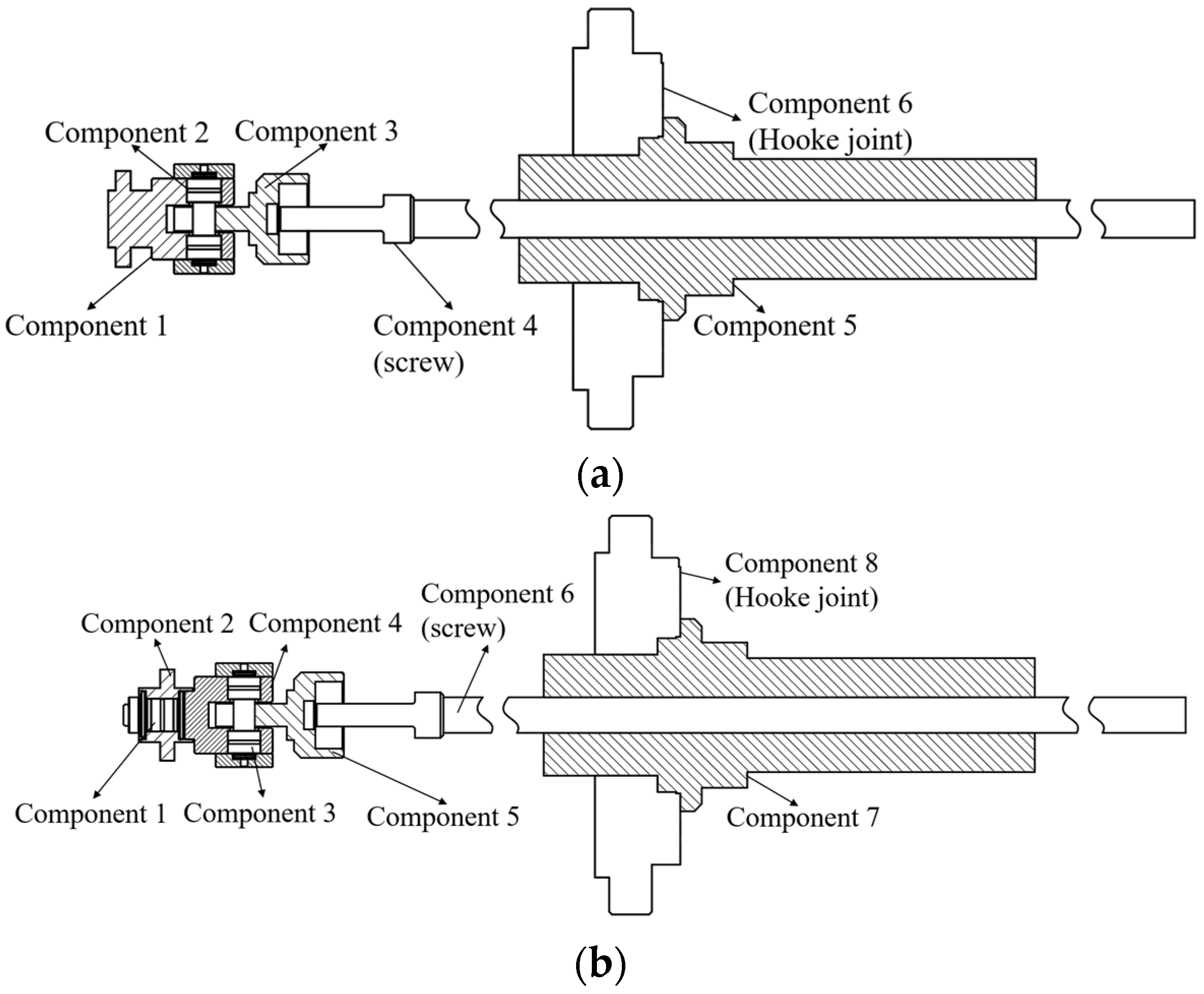
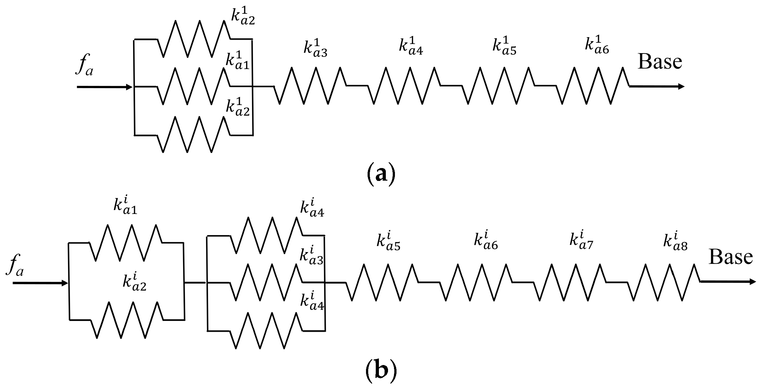
3.1.1. Stiffness Modeling of the Limbs

Assume that the base is rigid. According to the principle of virtual work, the virtual work done by the external load at the end effector of the five-axis parallel module is equal to the sum of the deformation energy of each limb. It can be written as

$${\mathit{\tau }}^{\mathrm{T}}{\Delta }_{\mathrm{p}}={\mathit{f}}^{\mathrm{T}}\Delta \mathit{\rho }$$

(14)

where $\mathit{\tau }$ represents the external load imposed on the end effector of the five-axis parallel module, ${\Delta }_{\mathrm{p}}$ represents the deformation of the end effector, f represents the actuation force and the constraint force, and $\Delta \mathit{\rho }$ represents the deformation in actuation and constraint directions. The relationship between f and $\Delta \mathit{\rho }$ can be written as

$$\begin{array}{l}\mathit{f}={\overline{\mathit{K}}}_{\rho }\Delta \mathit{\rho }\\ {\overline{\mathit{K}}}_{\rho }=\left(\begin{array}{cc}{\mathit{K}}_{\mathrm{a}}& 0\\ 0& K_{\mathrm{c}}\end{array}\right)\end{array}$$

(15)

where K_a and K_c are defined as the actuation stiffness matrix and the constraint stiffness, respectively. ${\overline{\mathit{K}}}_{\rho }$ is defined as the stiffness matrix of the limbs. Once Equations (8), (14), and (15) have been combined, the relationship between $\mathit{\tau }$ and ${\Delta }_{\mathrm{p}}$ can be written as

$$\begin{array}{l}\mathit{\tau }={\mathit{K}}_{\rho }{\Delta }_{\mathrm{p}}\\ {\mathit{K}}_{\rho }={{\mathit{J}}^{\prime }}^T{\overline{\mathit{K}}}_{\rho }{\mathit{J}}^{\prime }\end{array}$$

(16)

where K_ρ is defined as the stiffness matrix of the five-axis parallel module. The method to establish K_a and K_c will now be described in detail.

Because all the limbs are subjected to axial force only in actuation direction, K_a is a diagonal matrix. It can be written as

$${\mathit{K}}_{\mathrm{a}}=\mathit{diag}\left(k_{\mathrm{a}1}{,k}_{\mathrm{a}2}{,k}_{\mathrm{a}3}{,k}_{\mathrm{a}4}{,k}_{\mathrm{a}5}\right)$$

(17)

where k_ai (i = 1~5) denotes the axial stiffness coefficient of limb i, which is decided by the structure of the limb. The kinematic schemes of limb 1 (UCR kinematic chain) and limb 2~5 (UCU kinematic chain) are shown in Figure 9.

They can be simplified as the series spring systems, shown in Figure 10. Further, k_ai can be written as

$$\begin{array}{l}{k}_{\mathrm{a}1}{}^{-1}=(k_{\mathrm{a}1}^1+2k_{\mathrm{a}2}^1{)}^{-1}+{\displaystyle \sum _{j=3}^6{k}_{\mathrm{a}j}^1{}^{-1}}\\ k_{\mathrm{a}i}{}^{-1}=(k_{\mathrm{a}1}^i+k_{\mathrm{a}2}^i{)}^{-1}+(k_{\mathrm{a}3}^i+2k_{\mathrm{a}4}^i{)}^{-1}+{\displaystyle \sum _{j=5}^8{k}_{\mathrm{a}j}^i{}^{-1}}, i=2~5\end{array}$$

(18)

where $k_{\mathrm{a}6}^i\left(k_{\mathrm{a}4}^1\right)$ donates the axial stiffness of the screw, which is related to its length and $k_{\mathrm{a}8}^i\left(k_{\mathrm{a}6}^1\right)$ donates the equivalent translational stiffness of the Hooke joint along the axial direction of the limb, which is related to its pose. The other terms can be considered as constants. As shown in Figure 11, coordinate frame B-uvw attached to the Hooke joint inner ring takes the center of the Hooke joint as the coordinate origin, and coordinate frame B′-u′v′w′ attached to the Hooke joint outer ring has the same origin as coordinate frame B-uvw. The direction of each axis is also shown in Figure 11.

According to [10], the equivalent translational stiffness of the Hooke joint along the axial direction of the limb can be expressed as

$$k_{\mathit{epw}}{}^{-1}=k_{\mathit{pw}}{}^{-1}+{\mathit{w}}^{\mathrm{T}}{\mathit{R}}^{\prime }{{\mathit{K}}^{\prime }}_{\mathrm{p}}{{\mathit{R}}^{\prime }}^T\mathit{w}$$

(19)

where k_epw denotes the equivalent translational stiffness of the Hooke joint along the axial direction of the limb, k_pw denotes the axial stiffness of the Hooke joint inner ring in coordinate frame B-uvw, R′ denotes the rotation matrix of coordinate frame B′-u′v′w′, R″ denotes the rotation matrix of coordinate frame B-uvw, and ${{\mathit{K}}^{\prime }}_{\mathrm{p}}$ denotes the stiffness matrix of the Hooke joint outer ring in coordinate frame B′-u′v′w′.

K_c represents the bending stiffness of limb 1 and is not suitable to be solved in an analytical way, because of its complex structure [16]. Thus, the FEA-based method is used in this article. Limb 1 can be simply considered as a supported beam and is assumed to consist of an equal-section rod of length l and other components of constant stiffness in series. As shown in Figure 12, the equal-section rod of length l is in the middle of limb 1, and two constant stiffness components of lengths l₁₁ and l₁₂ are connected in series to its left and right, respectively.

The bending stiffness of limb 1 can be expressed as

$$K_{\mathrm{c}}=\frac{1}{C_1{l}^3{+C}_2{l}^2{+C}_3{l+C}_4}$$

(20)

By using the FEA method, K_c is obtained with a set of values of l. The least-squares method is used to fit coefficients C₁~C₄; the results are shown in

Table 1. Coefficients of constraint stiffness of limb 1.

Coefficients	C1	C2	C3	C4
Magnitude	2.26 × 10−7	−3.18 × 10−4	0.184	−33.0

. Once Equations (16)–(20) have been combined, the stiffness model of the limbs can be calculated.

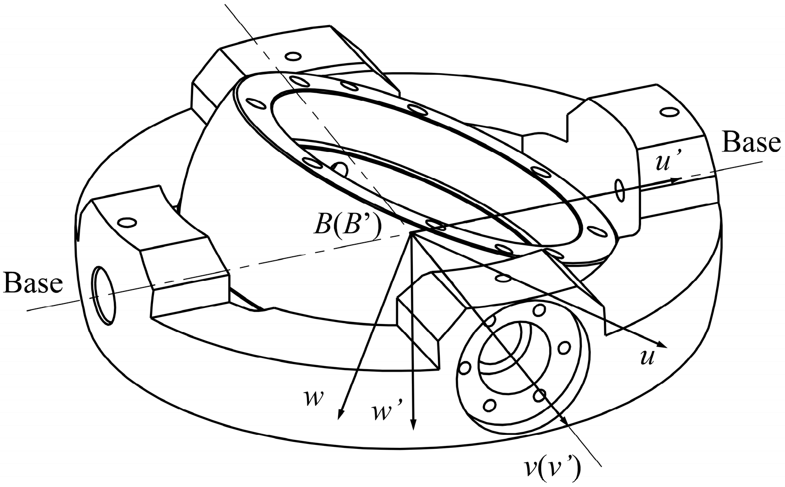
3.1.2. Stiffness Modeling of the Base

When the stiffness of the base and the stiffness of the limbs are in the same order of magnitude, the influence of base compliance on the stiffness of the end effector cannot be neglected. Therefore, the mapping relationship between them needs to be studied.

Assume that the limbs are rigid. The offset of the Hooke joint center is defined as $\Delta {\mathit{\rho }}_B$, which is a 15-order column vector. The generalized deformation of the end effector is defined as ${\Delta }_Q$, which is a six-order column vector. The relationship between $\Delta {\mathit{\rho }}_B$ and ${\Delta }_Q$ can be expressed as

$${\Delta }_Q={\mathit{J}}_{fB}\Delta {\mathit{\rho }}_B$$

(21)

According to the principle of virtual work, the virtual work done by the external load at the end effector of the five-axis parallel module is equal to the sum of the deformation energy of the base. It can be expressed as

$${\mathit{\tau }}_Q·{\Delta }_Q={\displaystyle \sum _{i=1}^5\Delta {\mathit{\rho }}_{\mathit{Bi}}·{\mathit{f}}_{\mathit{Bi}}=}\Delta {\mathit{\rho }}_B·{\mathit{f}}_B$$

(22)

where ${\mathit{\tau }}_Q$ represents the generalized external load of the end effector and f_B represents the load of the Hooke joint center.

According to Hooke’s law, the relationship between f_B and $\Delta {\mathit{\rho }}_B$ can be expressed by

$${\mathit{f}}_B={\overline{\mathit{K}}}_f\cdot \Delta {\mathit{\rho }}_B$$

(23)

where ${\overline{\mathit{K}}}_f$ is defined as the interface stiffness matrix of the base. Once Equations (22) and (23) have been combined, the stiffness matrix of the base mapped to the five-axis parallel module K_Qf can be expressed as

$$\begin{array}{l}{\mathit{\tau }}_Q={\mathit{K}}_{\mathit{Qf}}\cdot {\Delta }_Q\\ {\mathit{K}}_{\mathit{Qf}}=({\mathit{J}}_{fB}{\overline{\mathit{K}}}_f^{-1}{\mathit{J}}_{fB}^{\mathrm{T}}{)}^{-1}\end{array}$$

(24)

The FEA method is used to establish ${\overline{\mathit{K}}}_f$. The force model of the base subsystem is shown in Figure 13. ${\overline{\mathit{K}}}_f$ is chunked by column: ${\overline{\mathit{K}}}_f=({\overline{\mathit{K}}}_{f1} {\overline{\mathit{K}}}_{f2} {\overline{\mathit{K}}}_{f3} \cdots {\overline{\mathit{K}}}_{f15})$. Let $\Delta {\mathit{\rho }}_B$ be sequentially equal to e_i (e_i is a column vector whose ith element is 1, and the rest are 0), so that the corresponding support reaction force ${\mathit{p}}_{\mathrm{a}i}(i=1~15)$ can be calculated. So ${\overline{\mathit{K}}}_f$ can be constructed column by column as

$${\overline{\mathit{K}}}_{\mathit{fi}}={\mathit{p}}_{\mathrm{a}i}, (i=1~15)$$

(25)

According to linear superposition principle, the stiffness model of the end effector of the five-axis parallel module can be expressed as

$${\mathit{K}}_{PKM}={({\mathit{K}}_{\rho }^{-1}+{\mathit{K}}_{Qf}^{-1})}^{-1}$$

(26)

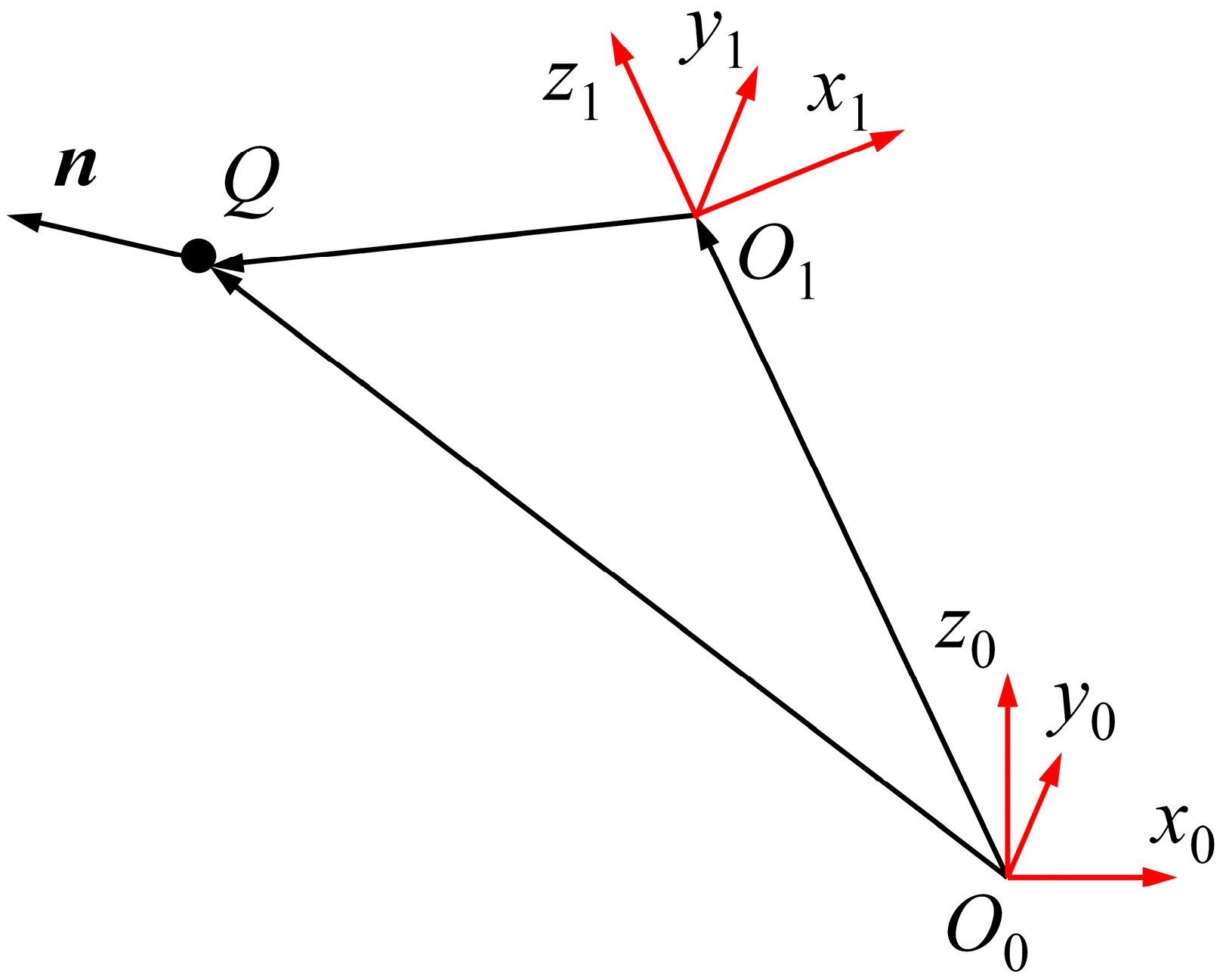
3.2. Stiffness Modeling of the Two-DoF Robotic Arm

When the stiffness of the robotic arm and the stiffness of the five-axis parallel module are of the same order of magnitude, its contribution to the stiffness of the hybrid machining robot cannot be neglected.

An MSA-based method is used to establish the stiffness model of the robotic arm. The stiffness matrix of each component in the local coordinate frame is defined as ${\mathit{K}}_i^e$ and can be obtained by using FEA software. The rotation matrix of each component is defined as ${\mathit{\lambda }}_i$ and can be calculated through the similar method mentioned in Section 2. Therefore, the stiffness matrix of component i in the global coordinate frame, O₀-x₀y₀z₀, can be expressed as

$$\begin{array}{l}{\mathit{K}}_i^{O_0}={\mathit{T}}_i{\mathit{K}}_i^e{\mathit{T}}_i^{\mathrm{T}}\\ {\mathit{T}}_i=\mathit{diag}(\underset{1}{{\mathit{\lambda }}_i} \underset{2}{{\mathit{\lambda }}_i}\cdots \underset{2k}{{\mathit{\lambda }}_i})\end{array}$$

(27)

where ${\mathit{K}}_i^{O_0}$ denotes the stiffness matrix of component i in the global coordinate frame, O₀-x₀y₀z₀.

The stiffness matrix of the robotic arm is defined as ${\mathit{K}}_{\mathit{limb}}^{+}$. It is a 188-order matrix and can be obtained from ${\mathit{K}}_i^{O_0}$ through order expansion and splicing. According to the displacement boundary conditions, the rows and columns of ${\mathit{K}}_{\mathit{limb}}^{+}$ with 0 generalized displacement are deleted. Then a 178-order matrix can be obtained, and it is defined as ${\mathit{K}}_{\mathit{limb}2}^{+}$. The corresponding force vector is defined as f, and the displacement vector is defined as δ. The relationship between them can be expressed as

$$\mathit{f}={\mathit{K}}_{\mathit{limb}2}^{+}\mathit{\delta }$$

(28)

To focus on the stiffness matrix of the end effector of the robotic arm, ${\mathit{K}}_{\mathit{limb}2}^{+}$ is chunked, and the center of the end effector of the robotic arm is defined as node 1. Therefore, Equation (28) can be expressed as

$$\left[\begin{array}{c}{\mathit{f}}_1\\ 0\end{array}\right]=\left(\begin{array}{cc}{\mathit{K}}_{11}& {\mathit{K}}_{12}\\ {\mathit{K}}_{21}& {\mathit{K}}_{22}\end{array}\right)\left[\begin{array}{c}{\mathit{\delta }}_1\\ {\mathit{\delta }}_{\mathrm{others}}\end{array}\right]$$

(29)

According to static coalescence, the relationship between f₁ and δ₁ can be expressed as

$$\begin{array}{l}{\mathit{f}}_1={\mathit{K}}_{limb}{\mathit{\delta }}_1\\ {\mathit{K}}_{limb}={\mathit{K}}_{11}-{\mathit{K}}_{12}{\mathit{K}}_{22}^{-1}{\mathit{K}}_{21}\end{array}$$

(30)

where f₁ denotes the external force imposed on the end effector of the robotic arm and δ₁ denotes the corresponding generalized displacement.

3.3. Stiffness Modeling of the Hybrid Machining Robot

Without loss of generality, the stiffness-modeling method for a hybrid robot with n subsystems connected in series is investigated. The scheme of a hybrid robot is shown in Figure 14. Q and n represent the position and orientation of the spindle, respectively. Q_i represents the center of the (i + 1)th subsystem’s end effector. The stiffness matrix of the nth subsystem in its local coordinate frame is defined as K_n, and the position of the nth subsystem end effector’s center in its local coordinate frame is defined as ${\left(x_n{,y}_n{,z}_n\right)}^{\mathrm{T}}$. The mapping matrix of the deformation of the nth subsystem’s end effector with respect to the deformation of the (n − 1)th subsystem’s end effector is ${R_n}^{\prime }$. The external force of the end of the hybrid robot is defined as F_Q, and the corresponding displacement is δ_Q. Meanwhile, the force on the nth subsystem’s coordinate origin caused by F_Q is defined as F_n, and the corresponding displacement is defined as δ_n. Assume that the nth subsystem is deformable and that the other subsystems are rigid. The relationship between δ_Q and δ_n can be expressed as

$$\begin{array}{l}{\mathit{\delta }}_Q={{\mathit{R}}_n}^{\prime }·{\mathit{\delta }}_n\\ {{\mathit{R}}_n}^{\prime }=\left(\begin{array}{cc}{\mathit{I}}_3& {\mathit{\lambda }}_n\\ 0& {\mathit{I}}_3\end{array}\right)\\ {\mathit{\lambda }}_n=\left(\begin{array}{ccc}0& z_n& -y_n\\ -z_n& 0& x_n\\ y_n& -x_n& 0\end{array}\right)\end{array}$$

(31)

where I₃ is a third-order unit matrix.

Thus, the mapping matrix of the deformation of the nth subsystem’s end effector with respect to the deformation of the hybrid robot’s end effector can be expressed as

$${\mathit{R}}_n={{\mathit{R}}_n}^{\prime }{{\mathit{R}}_{n-1}}^{\prime }\dots {{\mathit{R}}_2}^{\prime }$$

(32)

The principle of virtual work can be expressed as

$${\mathit{F}}_Q\cdot {\mathit{\delta }}_Q={\mathit{F}}_n·{\mathit{\delta }}_n$$

(33)

Once Equations (31)–(33) have been combined, the relationship between F_Q and δ_Q caused by the compliance of the nth subsystem can be expressed as

$$\begin{array}{l}{\mathit{F}}_Q={\mathit{K}}_{\mathrm{nf}}{\mathit{\delta }}_Q\\ {\mathit{K}}_{\mathrm{nf}}={\mathit{R}}_n^{-\mathrm{T}}{\mathit{K}}_n{\mathit{R}}_n^{-1}\end{array}$$

(34)

According to the linear superposition principle, the stiffness matrix of a hybrid robot with n subsystems connected in series can be expressed as

$${\mathit{K}}_Q^{-1}={\mathit{K}}_1^{-1}+{\displaystyle \sum _{i=2}^n({\mathit{R}}_i^{-\mathrm{T}}{\mathit{K}}_i}{\mathit{R}}_i^{-1}{)}^{-1}$$

(35)

For the hybrid machining robot, it comprises two subsystems: the five-axis parallel module and the robotic arm. ${{\mathit{R}}_0}^{\prime }$ and λ₀ can be expressed as

$$\begin{array}{l}{\mathit{R}}_0=\left(\begin{array}{cc}{\mathit{I}}_3& {\mathit{\lambda }}_0\\ 0& {\mathit{I}}_3\end{array}\right)\\ {\mathit{\lambda }}_0=\left(\begin{array}{ccc}0& z_1& -y_1\\ -z_1& 0& x_1\\ y_1& -x_1& 0\end{array}\right)\end{array}$$

(36)

According to Equations (34) and (35), the stiffness model of the hybrid machining robot can be expressed as

$$\begin{array}{l}{\mathit{K}}_h=({\mathit{K}}_{\mathit{PKM}}^{-1}+{\mathit{K}}_{\mathit{limbf}}^{-1}{)}^{-1}\\ {\mathit{K}}_{\mathit{limbf}}={\mathit{R}}_0^{-\mathrm{T}}{\mathit{K}}_{\mathit{limb}}{R}_0^{-1}\end{array}$$

(37)

where K_limbf represents the stiffness matrix of the robotic arm mapped to the end of the hybrid machining robot and K_h represents the stiffness matrix of the hybrid machining robot.

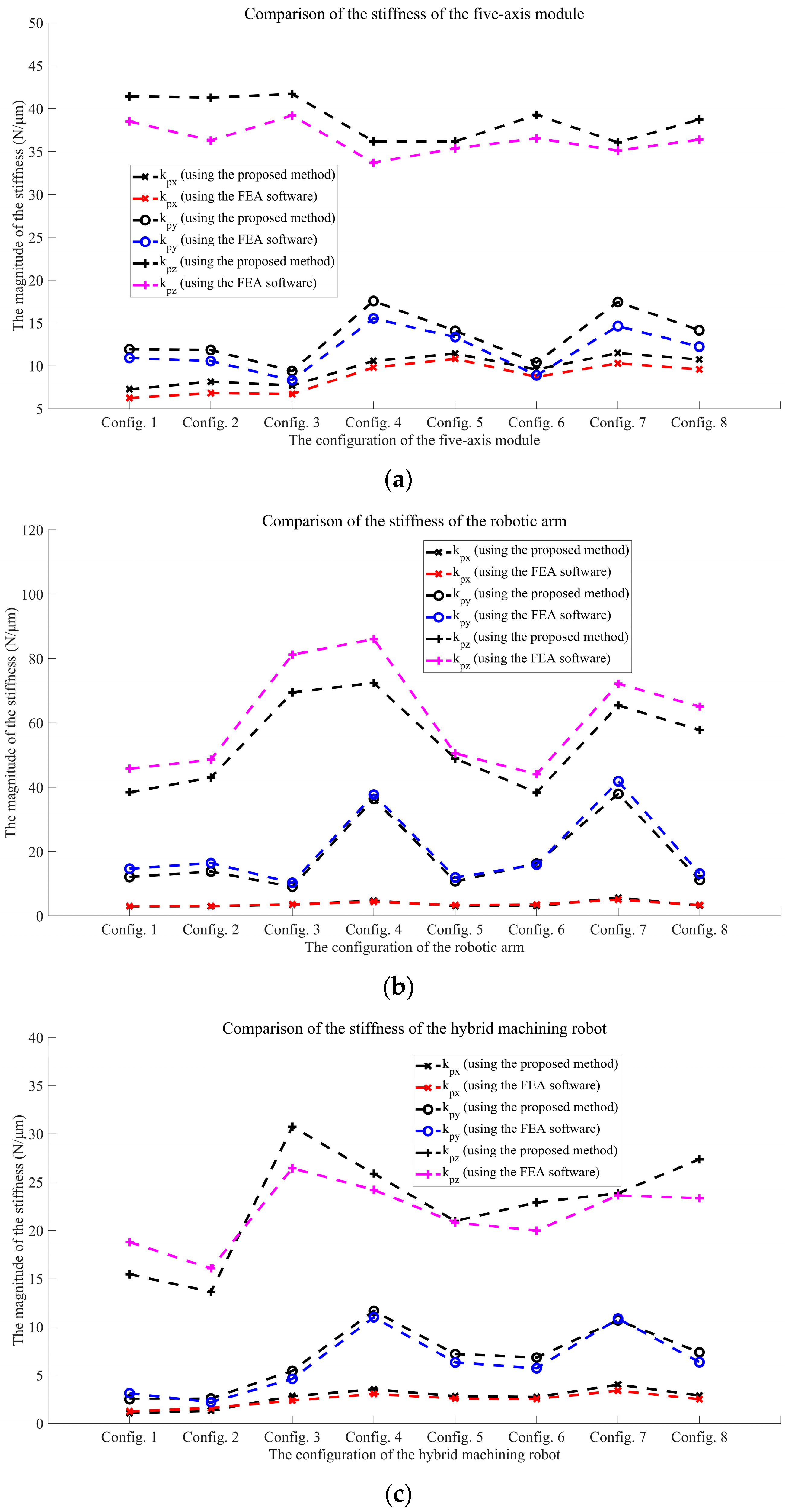
3.4. Simulation Experiment

A simulation experiment is carried out to verify the stiffness model. FEA software was used to calculate the stiffness in compared with that obtained by the method proposed in this article. Eight configurations of the five-axis parallel module, eight configurations of the robotic arm, and eight configurations of the hybrid machining robot were selected randomly as the validation configurations. The comparison of the stiffness of the five-axis module, the robotic arm, and the hybrid machining robot obtained by the two methods is shown in Figure 15a–c. According to the information in Figure 15, it can be concluded that the variation of stiffness obtained by the method proposed in this article has the same trend of that obtained by the FEA software. Therefore, the stiffness model has been verified, and it can be used to predict the trend of stiffness variation with configuration.

4. Stiffness-Performance Evaluation and Redundant Motion Planning

The hybrid machining robot consists of two subsystems connected in series, and the two-stage-positioning mode results in redundant DoFs in the y-direction and z-direction (shown in Figure 1), which makes it possible to optimize the robot’s configuration during machining. In [29,30], researchers proposed stiffness-performance indices and redundant motion-planning methods for drilling robots, and the stiffness of the robot in the feed direction is improved by optimizing the configuration. For the drilling processing, the stiffness performance in the plan perpendicular to the feed direction also has an impact on the hole quality. The previous research in this field is relatively limited. Therefore, redundant motion planning based on stiffness-performance indices still needs to be investigated.

4.1. Mathematical Description of Redundant Motion

According to Section 2, Equation (13) can be also expressed as

$$\left[\begin{array}{l}{x}_0\\ y_0\\ z_0\end{array}\right]=\left[\begin{array}{l}{x}_{O_1}\\ y_{O_1}\\ z_{O_1}\end{array}\right]+\mathit{R}\left[\begin{array}{l}{x}_1\\ y_1\\ z_1\end{array}\right], \left[\begin{array}{c}\cos f_0\sin {\theta }_0\\ \sin f_0\cos {\theta }_0\\ \cos {\theta }_0\end{array}\right]=\mathit{R}\left[\begin{array}{c}\cos f_1\sin {\theta }_1\\ \sin f_1\cos {\theta }_1\\ \cos {\theta }_1\end{array}\right]$$

(38)

where R is a three-order unit matrix and $x_{O_1}=0$. The pose of the hybrid machining robot can be expressed as ${[x_1,y_1,z_1,f_1,{\theta }_1,y_{O_1},z_{O_1}]}^{\mathrm{T}}$. Therefore, the following relationship can be obtained:

$$x_0=x_1,y_0=y_{O_1}+y_0,z_0=z_{O_1}+z_1,f_0=f_1,{\theta }_0={\theta }_1$$

(39)

According to Equation (39), when the position and the orientation of the spindle are given, only three of seven DoFs can be determined (x₁, f₁ and θ₁). Thus, the redundant motion-planning problem turns into obtaining the optimal configuration of the robot by optimizing the distribution for $y_1,z_1,y_{O_1},z_{O_1}$.

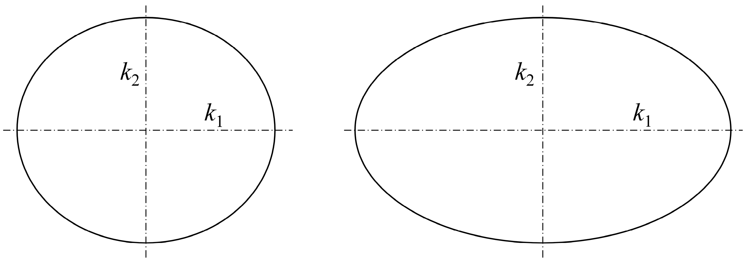
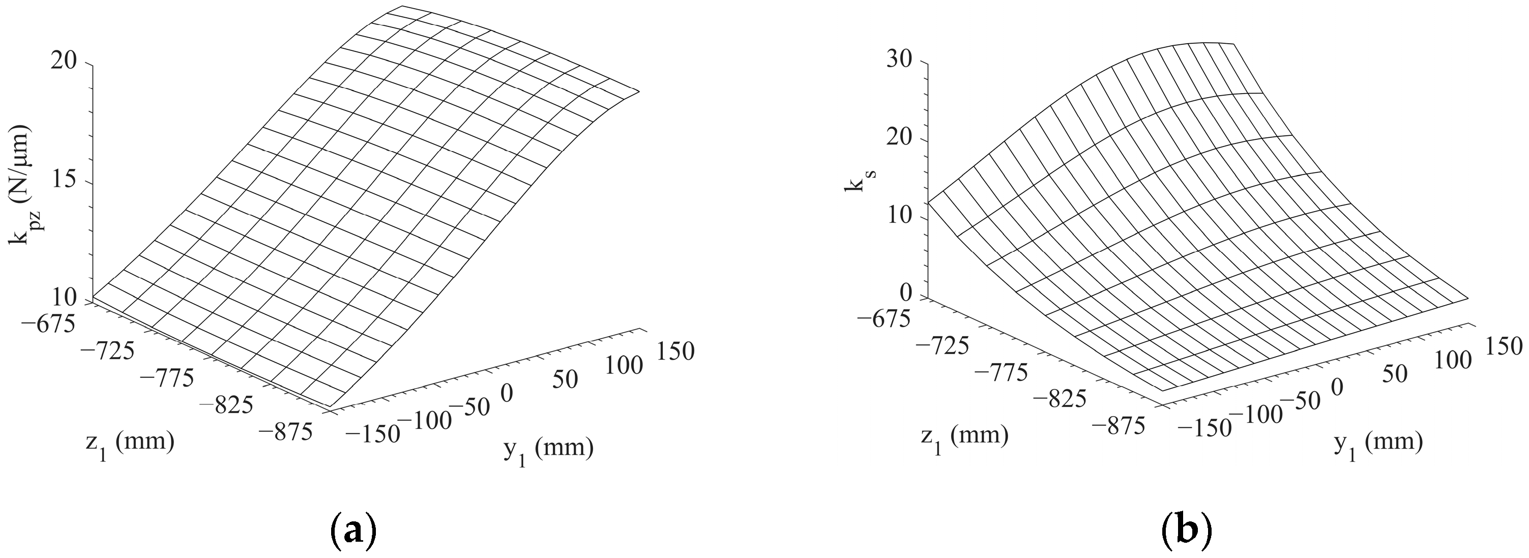
4.2. Stiffness Evaluation

To conduct a stiffness evaluation on the drilling process, it is necessary to analyze the force on the twist drill during processing. The force diagram of twist drill during processing is shown in Figure 16.

The generalized force applied to the twist drill is defined as ${[F_x F_y F_z M_x M_y M_z]}^{\mathrm{T}}$, where F_x, F_y, M_x, and M_y represent the generalized force in the radial plane and F_z and M_z represent the generalized force along the spindle axis. Theoretically, the generalized force can be expressed as

$$\begin{array}{l}{F}_x=F_y=0, M_x=M_y=0\\ F_z=F_{f\psi }+2F_{\mathit{fo}}+2F_{\mathit{fo}1}\\ M_z=M_{c\psi }{+M}_{\mathit{co}}{+M}_{\mathit{co}1}\end{array}$$

(40)

The cutting pressure applied on the end effector can be neglected when compared with the translational force [16]. Moreover, according to Equation (40), the magnitude of force along the spindle axis is much higher than that in the radial plane. Therefore, the axial stiffness along spindle axis k_pz has a significant influence on the accuracy of the hole axial direction, and it is defined as the axial stiffness index.

Meanwhile, there still exist forces in the radial plane because of nonideal conditions, such as the uneven distribution of material properties, the pose error of the twist drill, and the twist drill’s unevenly wearing. Thus, the stiffness performance in the radial plane needs to be accounted for [31]. The translational stiffness in the x’ direction and the y’ direction is defined as k_px and k_py, respectively. When the larger one is taken as the long axis of the ellipse and the other as the short axis, the centrifugal rate can be expressed as

$$\begin{array}{l}e=\sqrt{1-(k_2/k_1{)}^2}\\ k_1=\mathit{max}(k_{\mathrm{px}};k_{\mathrm{py}})\\ k_2=\mathit{min}\left(k_{\mathrm{px}}{;k}_{\mathrm{py}}\right)\end{array}$$

(41)

The centrifugal rate, e, characterizes the stiffness isotropy in the radial plane, and the closer the magnitude of k₁ and k₂ are, the closer the magnitude of e is to 0. To ensure drilling precision, the magnitude of k₁ and k₂ must be accounted for. Figure 17 shows two ellipses with the same short axis, and the latter one has a longer long axis. The diameter of the latter one is larger than that of the former one, in all directions, but its centrifugal rate is higher. Therefore, it is necessary to take the magnitude of k₁ and k₂ into account. In this article, the area of the ellipse is used to reflect the magnitude of k₁ and k₂, and the stiffness index in radial plane can be defined as

$$k_s=\pi k_1{k}_2/e$$

(42)

where k_s is the radial plane stiffness index and at the same time characterizes both the stiffness isotropy and the magnitude in the radial plane. Both an increase in k₁ and k₂ and an improvement in stiffness isotropy will increase k_s.

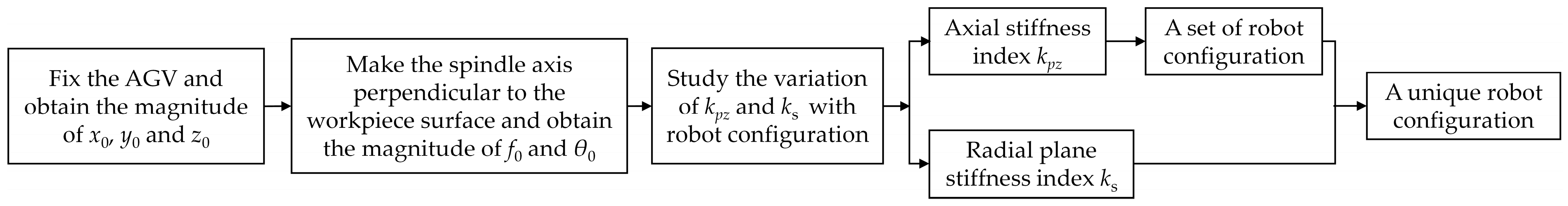
4.3. Redundant Motion Planning

According to the machining process mentioned in Section 2, the redundant motion-planning method can be summarized in five steps, shown in Figure 18:

(1)

Fix the AGV and obtain the magnitude of x₀, y₀, and z₀.

(2)

Make the spindle axis perpendicular to the workpiece surface by adjusting f and θ.

(3)

Figure out how k_pz and k_s vary with the configuration of the hybrid machining robot.

(4)

Select a set of robot configurations that make the magnitude of k_pz high.

(5)

Determine a unique robot configuration that makes the magnitude of k_s the highest among the robot configurations in Step 4.

4.4. Case Study

To better understand the redundant motion-planning method proposed in previous section, a case study is given. In this case, the parameters in Step 1 and Step 2 are set as following:

$$y_0=-750 \mathrm{mm},z_0=-1975 \mathrm{mm},x_1=x_0=0,f=0,\theta =0$$

(43)

When the position and the orientation of the spindle are given, the magnitudes of x₁, f, and θ are uniquely determined, and they will effect only J′, mentioned in Section 2. Therefore, even though x₁, f, and θ are not 0 when machining, the redundant motion-planning method still works.

The variation of the stiffness indices is shown in Figure 19. According to Figure 19a, k_pz is insensitive to the distribution of redundant motion in the z-direction and will increase as y₁ increases. Thus, a set of robot configurations that make the magnitude of k_pz high are where y₁ = 200 mm. Figure 19b shows that the higher the magnitude of y₁ and z₁ is, the higher the magnitude of k_s is. Therefore, in this case, the optimal configuration of the robot for drilling is y₁ = 200 mm, z₁ = −675 mm, y₀ = −950 mm, and z₀ = −1300 mm.

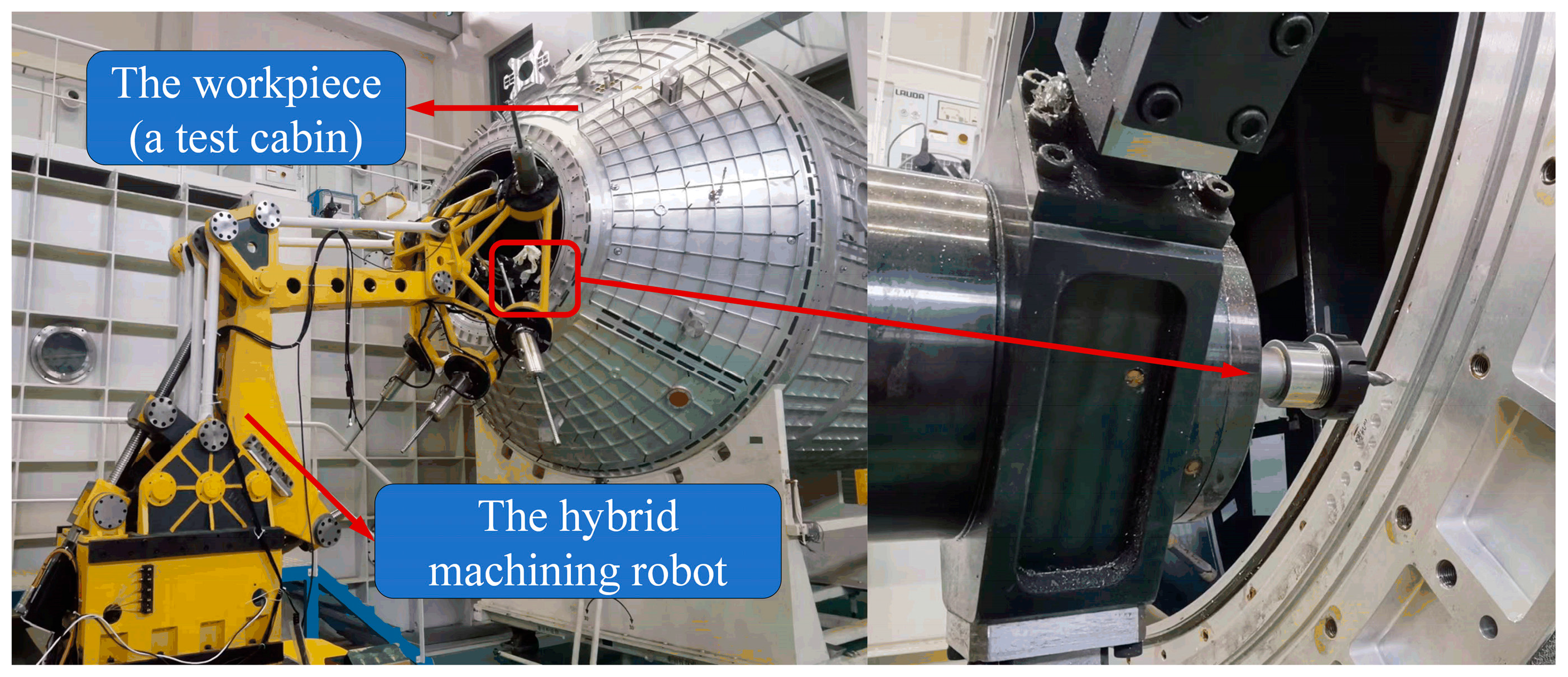
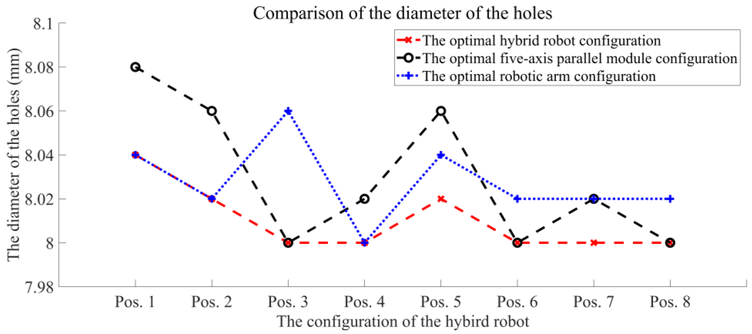
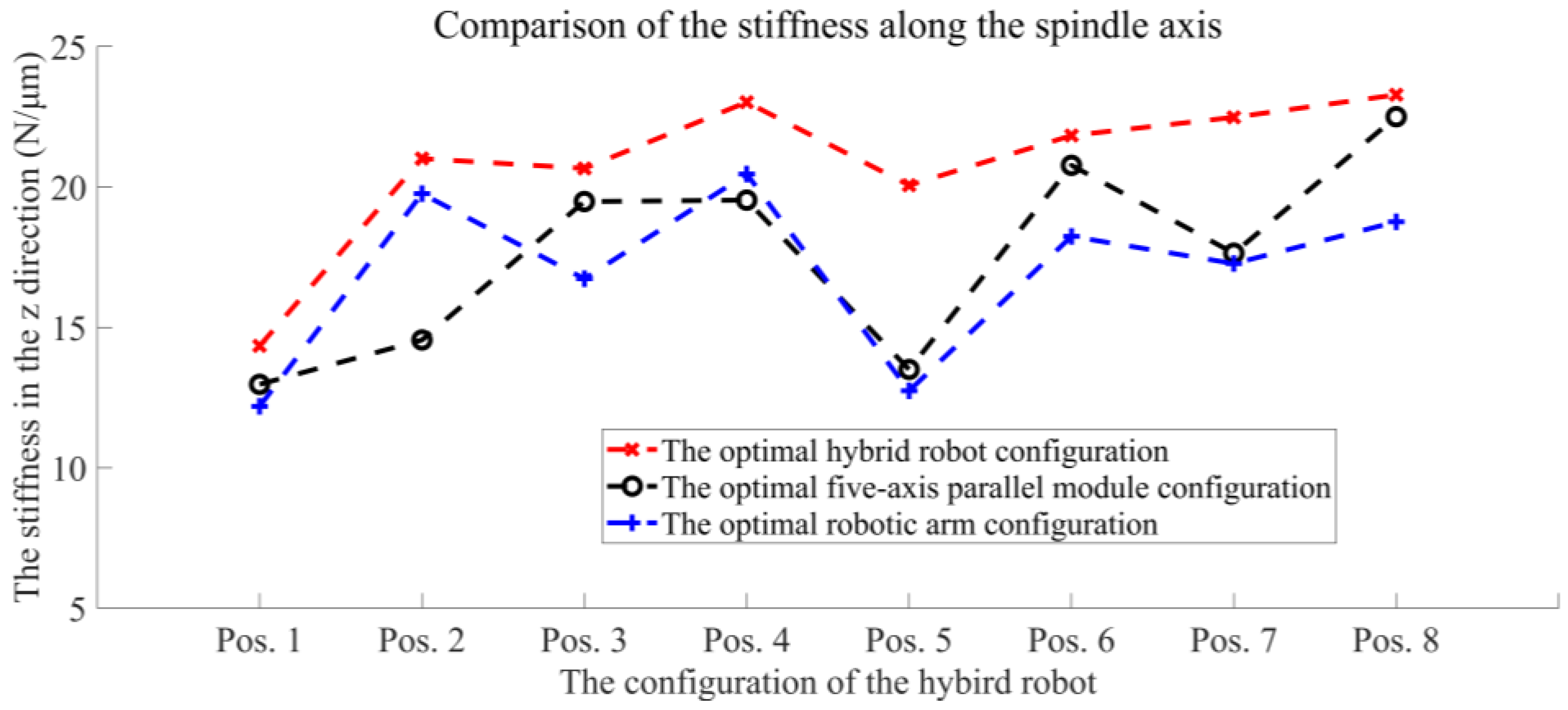
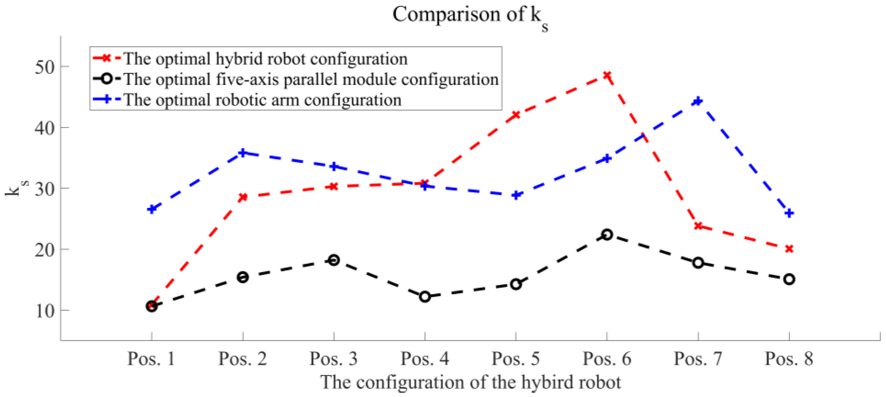
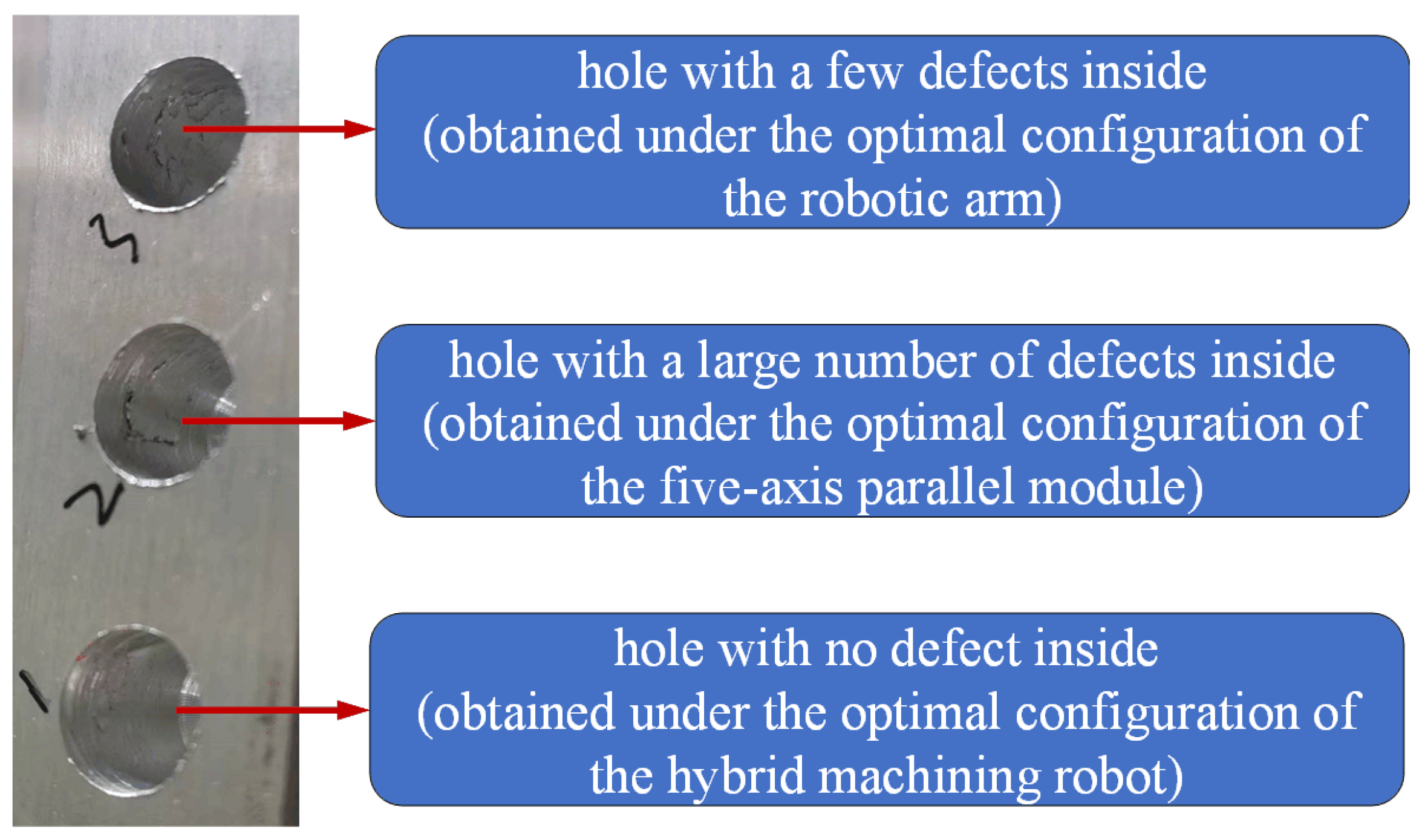
5. Drilling Experimental Verification

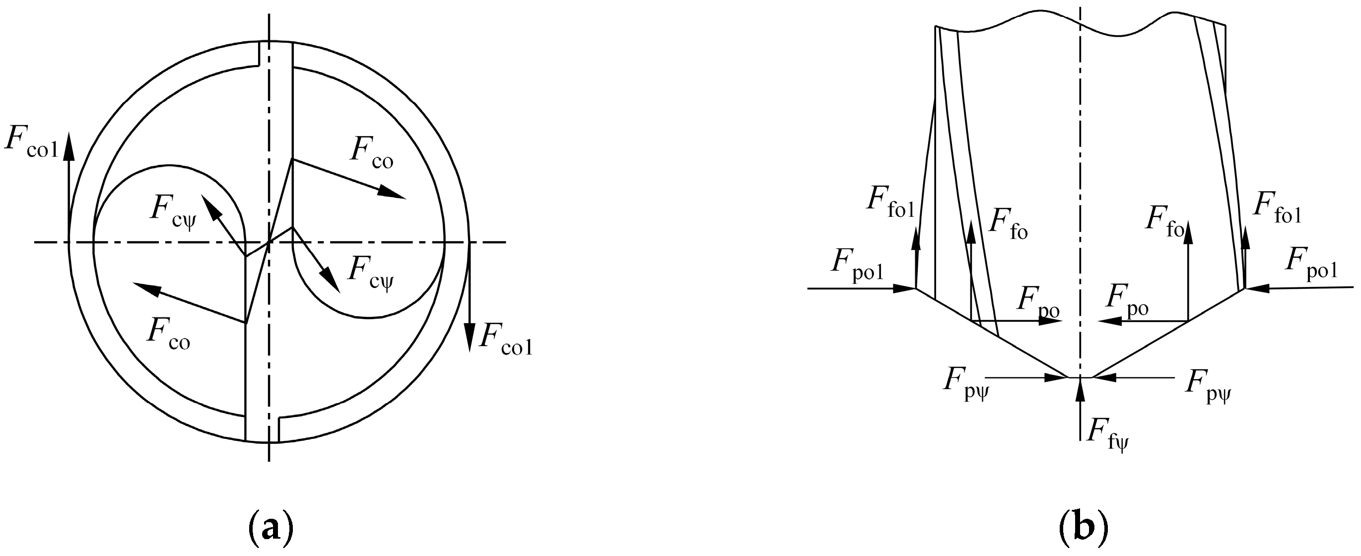
5.1. Design of Drilling Comparative Experiment

After establishing the stiffness model of the hybrid machining robot and proposing a redundant motion-planning method for drilling, it is necessary to conduct a drilling experiment to verify the validity of the proposed method. The hybrid machining robot and the workpiece (a test cabin made up of aluminum) used in the experiment are shown in Figure 20, and the test cabin has high relatively local stiffness at the end face. The AGV was moved to a suitable position and was fixed on the ground. Points in the workspace were selected randomly as drilling positions. For each position, the optimal configuration of the hybrid machining robot was determined by the five steps mentioned in Section 4.

To determine the optimal configuration of the hybrid machining robot, two other configurations are used for each drilling position. The five-axis parallel module contacts with the workpiece and has a direct impact on drilling precision. The robotic arm is away from the end effector of the hybrid machining robot, which means the deformation of it will be enlarged at the end and that the drilling precision will be influenced. Therefore, the two other configurations for comparison are based on the optimal configuration of the five-axis parallel module and the robotic arm, respectively. The error of the hole diameter is used to reflect the stiffness performance of the hybrid machining robot, because the stiffness of the robot is the ratio of force to the deformation of the end effector. When the forces applied to the end effector are the same, the higher the stiffness of the robot is, the smaller the error of the hole diameter is.

In this experiment, an 8 mm diameter drill was used for drilling, and federate was 60 mm/min. Eight drilling positions were selected, and holes were drilled in the end face of the test cabin. The vernier caliper was used to measure the diameter of the holes.

5.2. Experiment Result and Discussion

The diameters of the holes are shown in Figure 21, which demonstrates the difference in diameter of the holes drilled with different configurations in eight drilling positions. According to Figure 21, the mean diameters of the holes are 8.013 mm (with the optimal configuration of the hybrid machining robot, hereinafter called configuration 1), 8.030 mm (with the optimal configuration of the five-axis parallel module, hereinafter called configuration 2), and 8.028 mm (with the optimal configuration of the robotic arm, hereinafter called configuration 3). The relative errors of the diameters of the holes are 1.63% (with configuration 1), 3.75% (with configuration 2), and 3.50% (with configuration 3). It can be concluded that the error of the hole diameter obtained under the optimal configuration of the hybrid machining robot is smaller than those obtained under the other two configurations.

Figure 22 and Figure 23 show the stiffness of the hybrid machining robot along the spindle axis and the radial plane stiffness index, k_s, with different configurations in eight drilling positions, respectively. After combining these figures with Figure 21, the results in Pos. 3 and Pos. 7 show that although the magnitude of k_s with configuration 2 is lower than that with configuration 3, the diameter of the hole drilled with configuration 2 is not bigger than that drilled with configuration 3. According to the results in Pos. 1 and Pos. 5, although the magnitude of the stiffness along the spindle axis with configuration 2 is close to that with configuration 3, the diameter of the holed drilled with configuration 3 is smaller than that drilled with configuration 2. In conclusion, when the magnitude of the stiffness along the spindle axis is high, the diameter of the holes is influenced mainly by the stiffness along the spindle axis, despite the difference in the magnitude of k_s with different configurations, but the difference in the magnitude of k_s will lead to the difference of the diameter of the holes when the magnitude of the stiffness along the spindle axis is low.

The different machining performance with different robot configurations can be directly reflected by Figure 24. It demonstrates that there is no defect inside the hole drilled with the optimal configuration of the hybrid machining robot, whereas the holes drilled with the two other configurations have defects inside.

6. Conclusions

Motivated by the requirement for efficiently and precisely drilling in large-scale components, this article addressed the problem of the redundant motion planning of a hybrid machining robot on the basis of stiffness performance. The hybrid machining robot consists of two subsystems (a five-axis parallel module and a two-DoF (Degree-of-Freedom) robotic arm when the guideway is fixed). The kinematic analysis of the five-axis parallel module, the robotic arm, and the hybrid machining robot was carried out. To take the compliance of each subsystem into account, the stiffness-modeling method for the hybrid robot with n subsystems connected in series was proposed. The stiffness model of the hybrid robot was established using this method, and the variation of the stiffness magnitude had the same trend as that obtained by the FEA software. Based on the stiffness model, two stiffness indices were proposed. One (k_pz) was the stiffness magnitude along the spindle axis. The other (k_s) was defined as the ratio of the area to the centrifugal rate of the ellipse obtained by stiffness model, and it was used to evaluate stiffness isotropy in the radial plane. The redundant motion of the hybrid machining robot was planned by maximizing the stiffness magnitude along the spindle axis, with priority to the value of k_s. Finally, a drilling comparison experiment was carried out, and the results demonstrated that the error of the hole diameter obtained under the optimal configuration of the hybrid machining robot was smaller than those obtained under the other two configurations. The results also indicated that the diameter of the holes was influenced mainly by the stiffness of the hybrid machining robot along the spindle axis, and the effect of k_s on the diameter of the holes only showed up when the magnitude of the stiffness along the spindle axis was low. The proposed stiffness-modeling method and the stiffness-performance index were also applicable to other hybrid robots.

References

- Lei, P.; Zheng, L.Y. An automated in-situ alignment approach for finish machining assembly interfaces of large-scale components. Robot. Comput. Integr. Manuf. 2017, 46, 130–143. [Google Scholar] [CrossRef]
- Zhao, X.; Tao, B.; Ding, H. Multimobile Robot Cluster System for Robot Machining of Large-Scale Workpieces. IEEE ASME Trans. Mechatron. 2022, 27, 561–571. [Google Scholar] [CrossRef]
- Chen, K.X. A Thesis Submitted in Partial Fulfillment of the Requirements for the Degree for the Master of Engineering. Master’s Thesis, Huazhong University of Science & Technology, Wuhan, China, 2021. [Google Scholar]
- Tao, B.; Zhao, X.W.; Ding, H. Mobile-robotic machining for large complex components: A review study. Sci. China. Tech. Sci 2019, 62, 1388–1400. [Google Scholar] [CrossRef]
- Zhao, X.; Tao, B.; Han, S.; Ding, H. Accuracy analysis in mobile robot machining of large-scale workpiece. Robot. Comput. Integr. Manuf. 2021, 71, 102153. [Google Scholar] [CrossRef]
- DeVlieg, R.; Sitton, K.; Feikert, E.; Inman, J. ONCE (ONe-sided Cell End effector) robotic drilling system. In Proceedings of the 2002 SAE Automated Fastening Conference & Exhibition, Chester, UK, 1–3 October 2002. [Google Scholar]
- Zhang, Z.Y.; Jiang, Q. Research on integration technology of wing box robot drilling system for large aircraft. Aeros. Manuf. Tech. 2018, 61, 16–23. [Google Scholar]
- Brahmia, A.; Kelaiaia, R.; Company, O.; Chemori, A. Kinematic sensitivity analysis of manipulators using a novel dimensionless index. Rob. Auton. Syst. 2022, 150, 104021. [Google Scholar] [CrossRef]
- Metrom. Available online: https://metrom.com/on-site-machining-robot/ (accessed on 3 September 2022).
- Wang, Y.Y. Stiffness Modeling Theory and Approach of the Spherical Coordinate Hybrid Robot. Ph.D. Thesis, Tianjin University, Tianjin, China, 2008. [Google Scholar]
- Xie, F.G.; Mei, B.; Liu, X.J.; Zhang, J.B.; Yue, Y. Novel mode and equipment for machining large complex components. J. Mech. Eng. 2020, 56, 70–78. [Google Scholar]
- Brahmia, A.; Kelaiaia, R.; Chemori, A.; Company, O. On Robust Mechanical Design of a PAR2 Delta-Like Parallel Kinematic Manipulator. J. Mech. Robot. 2022, 14, 11001. [Google Scholar] [CrossRef]
- Jiao, J.C.; Tian, W.; Liao, W.H.; Zhang, L.; Bu, Y. Processing configuration off-line optimization for functionally redundant robotic drilling tasks. Robot. Auton. Syst. 2018, 110, 112–123. [Google Scholar] [CrossRef]
- Yan, S.J.; Ong, S.K.; Nee, A.Y.C. Stiffness analysis of parallelogram-type parallel manipulators using a strain energy method. Robot. Comput. Integr. Manuf. 2016, 37, 13–22. [Google Scholar] [CrossRef]
- Shanmugasundar, G.; Sivaramakrishnan, R.; Meganathan, S.; Balasubramani, S. Structural optimization of a five degrees of freedom (T-3R-T) robot manipultor using finite element analysis. Mater. Today Proc. 2019, 16, 1325–1332. [Google Scholar] [CrossRef]
- Klimchik, A.; Pashkevich, A.; Chablat, D. Fundamentals of manipulator stiffness modeling using matrix structural analysis. Mech. Mach. Theory 2019, 133, 365–394. [Google Scholar] [CrossRef]
- Delblaise, D.; Hernot, X.; Maurine, P. A systematic analytical method for PKM stiffness matrix calculation. In Proceedings of the 2006 IEEE International Conference on Robotics and Automation, Orlando, FL, USA, 15–19 May 2006. [Google Scholar]
- Cammarata, A. Unified formulation for the stiffness analysis of spatial mechanisms. Mech. Mach. Theory 2016, 105, 272–284. [Google Scholar] [CrossRef]
- Yu, G.; Wang, L.P.; Wu, J.; Wang, D.; Hu, C.J. Stiffness modeling approach for a 3-DOF parallel manipulator with consideration of nonlinear joint stiffness. Mech. Mach. Theory 2018, 123, 137–152. [Google Scholar] [CrossRef]
- Gosselin, C. Stiffness mapping for parallel manipulators. IEEE Trans. Robot. Autom. 1990, 6, 377–382. [Google Scholar] [CrossRef]
- Zhao, C.; Guo, H.W.; Zhang, D.; Liu, R.Q.; Li, B.; Deng, Z.Q. Stiffness modeling of n(3RRlS) reconfigurable series-parallel manipulators by combining virtual joint method and matrix structural analysis. Mech. Mach. Theory 2020, 152, 103960. [Google Scholar] [CrossRef]
- Görgülü, İ.; Carbone, G.; Dede, M.İ.C. Time efficient stiffness model computation for a parallel haptic mechanism via the virtual joint method. Mech Mach Theory 2020, 143, 103614. [Google Scholar] [CrossRef]
- Cao, W.; Yang, D.; Ding, H. A method for stiffness analysis of overconstrained parallel robotic mechanisms with Scara motion. Robot. Comput. Integr. Manuf. 2018, 49, 426–435. [Google Scholar] [CrossRef]
- Chen, J.K.; Xie, F.G.; Liu, X.J.; Bi, W.Y. Stiffness evaluation of an adsorption robot for large-scale structural parts processing. J. Mech. Robot. 2021, 13, 40907. [Google Scholar] [CrossRef]
- Wang, M.M.; Luo, J.J.; Fang, J.; Yuan, J.P. Optimal trajectory planning of free-floating space manipulator using differential evolution algorithm. Adv. Space Res. 2018, 61, 1525–1536. [Google Scholar] [CrossRef]
- Nouri Rahmat Abadi, B.; Mahzoon, M.; Farid, M. Singularity-free trajectory planning of a 3-RPRR planar kinematically redundant parallel mechanism for minimum actuating effort. Iran. J. Sci. Technol. Trans. Mech. Eng. 2019, 43, 739–751. [Google Scholar] [CrossRef]
- Chembuly, V.V.M.J.; Voruganti, H.K. Trajectory planning of redundant manipulators moving along constrained path and avoiding obstacles. Procedia Comput. Sci. 2018, 133, 627–634. [Google Scholar] [CrossRef]
- Liao, Z.Y.; Li, J.R.; Xie, H.L.; Wang, Q.H.; Zhou, X.F. Region-based toolpath generation for robotic milling of freeform surfaces with stiffness optimization. Robot. Comput. Integr. Manuf. 2020, 64, 101953. [Google Scholar] [CrossRef]
- Bu, Y.; Liao, W.H.; Tian, W.; Zhang, L.; Dawei, L.I. Modeling and experimental investigation of Cartesian compliance characterization for drilling robot. Int. J. Adv. Manuf. Technol. 2017, 91, 3253–3264. [Google Scholar] [CrossRef]
- Bu, Y.; Liao, W.H.; Tian, W.; Zhang, J.; Zhang, L. Stiffness analysis and optimization in robotic drilling application. Precis. Eng. 2017, 49, 388–400. [Google Scholar] [CrossRef]
- Görgülü, İ.; Dede, M.İ.C. A new stiffness performance index: Volumetric isotropy index. Machines 2019, 7, 44. [Google Scholar] [CrossRef] [Green Version]