1. Introduction
With the development of heavy-duty gas turbines, the mass flow rate and single-stage load of compressors and the alternating aerodynamic force borne by blades continue to rise, resulting in increasingly prominent fluid-induced blade vibration [
1]. The vibration problems faced by compressor blades mainly include the flutter and forced vibration caused by intake distortion [
2,
3], rotor–stator interference [
4,
5], stall and surge [
6,
7], and drop vortex [
8,
9]. The accidents caused by the forced vibration of gas turbines account for 25% of the total blade accidents, which cannot be ignored [
10]. However, due to its large flow rate and low speed, the first stage blade of the heavy-duty gas turbine is extremely long and, thus, prone to serious fatigue phenomenon and fracture failure.
Among the aerodynamic excitation factors, rotor–stator interaction is the inherent factor of compressors. The unsteady aerodynamic load caused by the rotor–stator interaction in an axial compressor is primarily because of the nonuniform potential flow field of adjacent blades and the viscous wake of upstream blades [
11,
12]. Michael [
13] found that wake is the main cause of blade surface pressure variation through a test study of a four-stage low-speed compressor. Vahdati et al. [
14] found that nonuniform potential flow field and viscous wake have significant effects on blade vibration in high pressure turbines. Bauer et al. [
15] studied the excitation characteristic of a radialflow turbine with an adjustable guide vane and pointed out that rotor–stator interaction is the main cause of compressor blade vibration under design conditions. At present, most of the research on the forced vibration caused by rotor–stator interaction focuses on single- or multi-stage compressors, but the forced vibration caused by struts is small.
The strut is an important part of heavy gas compressors and usually has few blades and a large thickness. Some researchers have studied the aerodynamic and vibration performance of struts for gas turbines. In terms of vibration, Chiang et al. [
16] found through a decoupled two-dimensional numerical simulation that struts cause significant potential flow disturbance on and the vibration of the final stage stator blade. Jones et al. [
17] simulated the rotor–stator–strut flow field through the potential flow model and found that the struts cause obvious nonuniform potential flow, which leads to the change in the stator blade force. Walker et al. [
18] studied the influence of the outlet struts’ shape on the aerodynamic performance of large civil turbofan engines through tests, and the optimized struts profile reduced the loss and the sensitivity to off-design working conditions. In terms of aerodynamics, Cioffi et al. [
19] proposed a new robust optimization method for compressor blades and applied it to the optimal design of inlet struts for heavy multistage axial compressors. Walker et al. [
20] used the outline of the existing intake struts and modified its arc line to improve the efficiency of the multistage compressor, and compared the flow field before and after optimization through three-dimensional CFD simulation. Turner et al. [
21] predicted the qualitative and quantitative features of the non-synchronous vortex that was shed in time by the interaction of the rotor shock with the trailing edge of the upstream strut. At present, the research on the excitation and vibration caused by the intake struts of heavy-duty gas turbines is limited.
In heavy-duty gas turbines, the inlet guide vanes and the first-stage rotor blades are usually located downstream of the intake struts, and their circumferential relative positions are fixed. Given that the number of inlet guide vanes and first-stage stator blades is usually not multiple or even mutual, the fundamental frequency and low octave excitations caused by two rows of blades are usually not superimposed, while the frequency of high octave excitations caused by the same frequency load of the two rows of blades is very high due to the large number of blades in the two rows, and the high order mode vibration is usually small. Therefore, the superposition effect of inlet guide vanes and the first-stage stator blades excitation has little influence on the rotor blades’ strength. However, the thick struts will generate a strong wake, which will transmit downstream for a long distance. Meanwhile, the number of struts is small, and the high frequency doubling may be the same as the low frequency doubling of the stator and the guide blades, which together will cause dangerous resonance.
In engineering, the Campbell diagram and blade frequency modulation are usually used to avoid the low-order resonance caused by struts, and a non-equidistant misfrequency design is adopted to reduce the excitation level of the multiple frequency of struts [
22]. However, these methods cannot completely eliminate the unsteady load of the relevant frequency and generate other frequency components to excite the first-stage rotor blades, together with the downstream stator blades and inlet guide vanes, complicating the excitation of the first-stage rotor blade. Therefore, the influence of struts and downstream stator blades and inlet guide vanes on the excitation and vibration of first-stage rotor blades should be considered.
When the circumferential relative positions of intake struts, inlet guide vanes, and first-stage blades are different, the excitation and vibration of the first-stage rotor blades are superimposed to different degrees, which belongs to the timing effect. At present, most of the studies on the timing effect in unsteady excitation are focused on stationary blades at different stages. Cizmas and Key [
23] found that when inlet guide vanes and stator blades are in a relatively high efficiency position, the guide vanes strengthen the pressure response of the stator blade and increase the potential flow interaction of the rotor and stator blades. Li and He [
24] studied the timing effect of rotor and stator blades in a 1.5-stage nonrepetitive turbine and found that changing the positions of rotor and stator blades effectively reduces the excitation level of blades. Lee [
25] studied the timing effect of rotor blades on the unsteady aerodynamic force of stationary blades through numerical simulation and found that the timing effect reaches 15%. Salontay and Key [
26,
27] conducted tests and numerical simulations on Purdue University’s three-stage low-speed axial flow compressor and found that the change in the excitation amplitude of the rotor blade suction surface reaches 37% because of the change in the static blade position.
In previous studies on the influence of blade position on unsteady excitation, the influence of intake struts was rarely considered. The thick intake strut is relatively stationary with the inlet guide vane and the stator blade, increasing the complexity of the unsteady load and vibration of the first-stage rotor blade, which needs further research. This paper takes the first 1.5-stage of a gas turbine compressor with intake struts as the object to study the influence law of the circumferential position of intake struts on the load and vibration of first-stage rotor blades under design conditions. This study can provide reference and guidance for the installation of compressor intake struts.
2. Materials and Methods
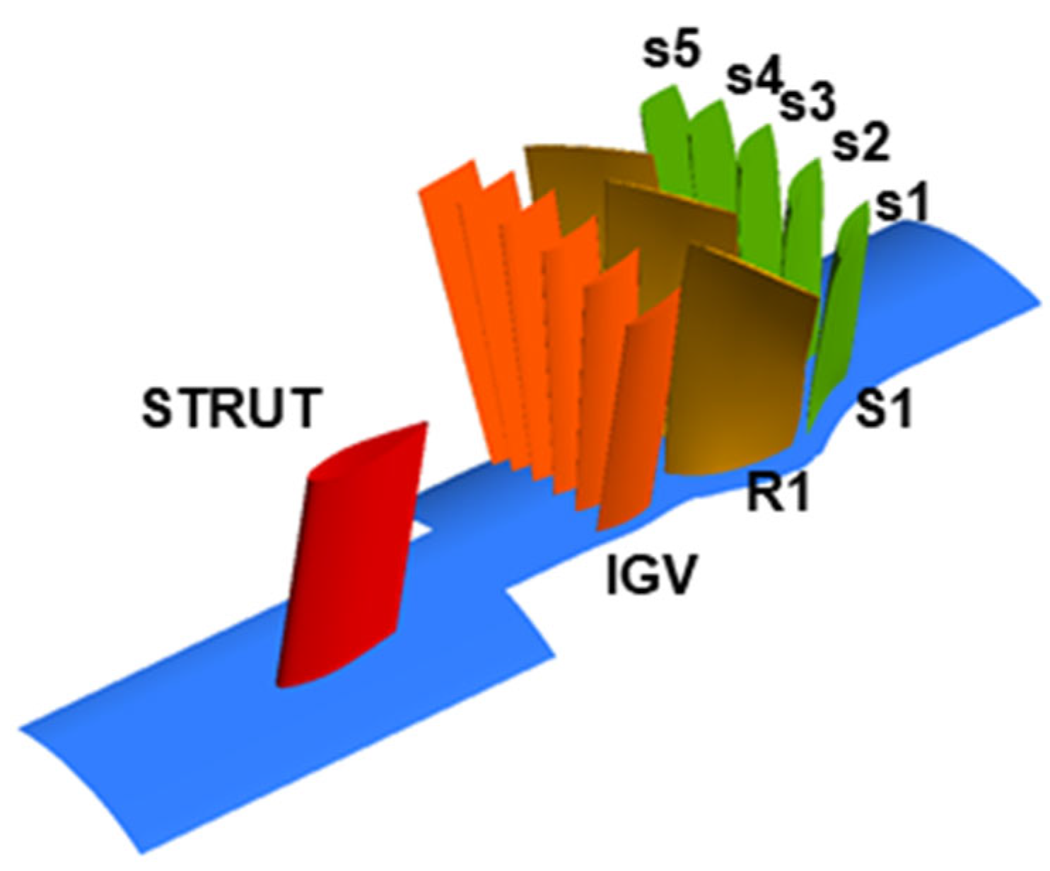
The research object is the first 1.5-stage of a compressor, including the inlet struts (STRUT), the inlet guide vanes (IGV), the first-stage rotor blades (R1), and the first-stage stator blades (S1), and the outlet is located at 2.5 times the chord length downstream of the S1 trailing edge. The tip clearance of R1 and S1 is 0.5 mm. The design speed is 9000 rpm.
To reduce the computational mesh number and save in computational cost, the numbers of STRUT, IGV, R1, and S1 are respectively reduced to 9, 54, 27, and 45, and 1/9 sector is used for calculation. The ratio of the numbers of blades in the computational domain is 1:6:3:5. When adjusting the number of blades, the blade profile size is scaled to ensure constant cascade solidity [
28,
29]. The blade profiles of the intake struts and the IGV are scaled with their trailing edge points as reference points, the previous edge point of the blades of S1 is scaled as the reference point to ensure that the axial distance from the trailing edge of the struts to the leading edge of R1 remains unchanged, and the axial clearance of IGV\R1 and R1\S1 remains unchanged. The blades of S1 are labelled s1, s2, s3, s4, and s5 along the counterclockwise direction of the flow direction. The geometric model is shown in
Figure 1.
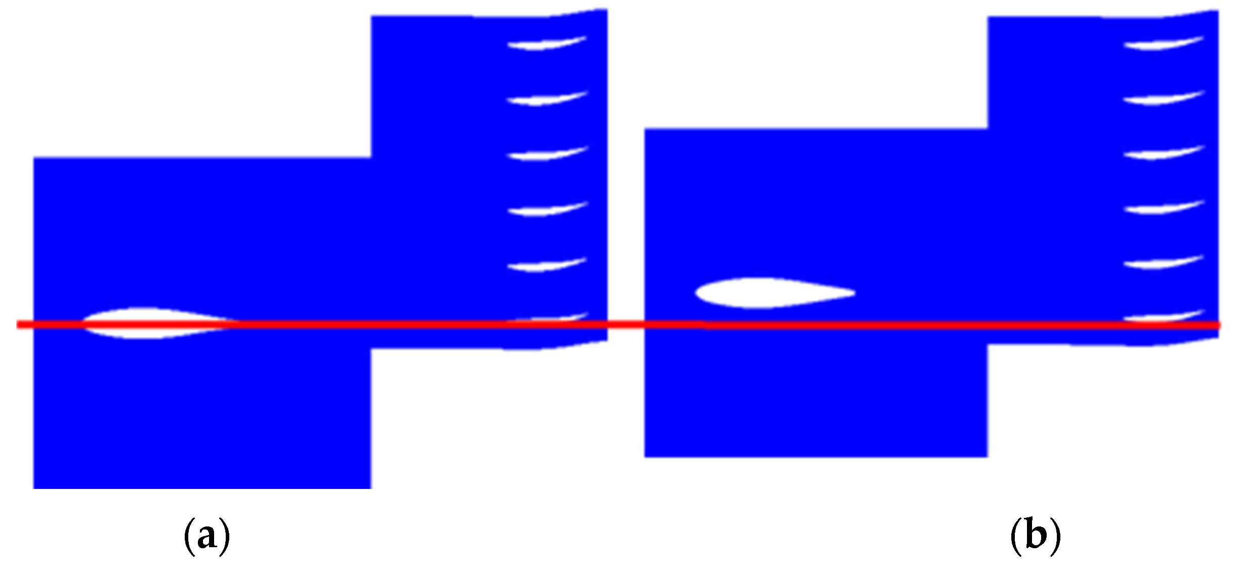
To study the influence of the different circumferential positions of the struts on the blade load and vibration, this paper sets two calculation examples according to the relative positions of the struts and the IGV, namely, C# and M#, respectively, as shown in
Figure 2. Viewed from the inlet along the axial downstream direction, the trailing edge of the struts in the C# example is axial to the leading edge of the IGV, while the trailing edge of the struts in the M# example is in the middle of the two leading edges of the IGV.
2.1. Mathematical Model
2.1.1. Fluid Model
The unsteady, compressible Reynolds-averaged Navier–Stokes equations are solved. This system of equations, written in a conservative form for a smoothly bounded control volume Ω with boundary Γ, takes the form:
where
i is the coordinate direction index, and
ni represents the
i-th direction component of the outward unit vector of the control volume boundary Γ.
U,
F,
G, and
S represent conservative vector, inviscid flux vector, viscous flux vector, and source term vector, respectively.
2.1.2. Structural Model
It is implicitly assumed that the vibration amplitude remains within the bounds of linear behavior. The structural motion equation can be written as:
where
M,
K, and
C are the mass, stiffness, and damping matrices;
x is the displacement vector;
f is a vector of pressures. A standard structural finite-element formulation is used to obtain the left-hand side, while the flow model above is used to obtain the unsteady forcing of the right-hand side.
To decouple the equations of motion for the damped systems, we use the mass normalized mode shape (
), defined as the normal modes divided by square root of the generalized mass (
). Let:
Equation (2) by the transpose Φ
T is:
where
.
q is the vector of the principal coordinates. N is the number of modal coordinates.
ωj and
ξj are natural frequency and modal damping ratio for mode
j.
When the external force is harmonic, under a single excitation frequency, Equation (4) can be transformed into:
where
ωex is excitation frequency, and
i is an imaginary unit. The subscript harmonic represents the harmonic components number of a variable at a specified frequency. By obtaining the harmonic components of the excitation force at the specified frequency, the displacement components of different mode shapes can be obtained, and the actual vibration displacement at the specified frequency can be obtained by superimposing them.
2.1.3. Vibration Calculation Method
The three-dimensional numerical methods for calculating blade vibration can be divided into coupling and decoupling methods. In the coupling method, the vibration of the blade in the fluid is calculated simultaneously, and the flow and structural fields transmit data to each other at each time step. The coupling method can fully simulate the coupling between the fluid and the solid with few assumptions, but it has a high computational cost and a slow convergence, especially near the resonance point.
The decoupling method calculates the vibration force and aerodynamic damping of the blade and provides the mechanical damping through the test results or experience. Excitation force, aerodynamic damping, and mechanical damping are applied to the structural calculation model of the blade, and the vibration of the blade is obtained through the transient or harmonic response calculation. This method considers the larger rigidity and density of the blade than those of the surrounding fluid and the small amplitude. The vibration shape of the fluid is basically unaffected by the aerodynamic load. Meanwhile, the influence of blade vibration on the surface excitation force can be ignored, and the excitation force and the aerodynamic damping can be solved separately [
30,
31]. The decoupling method is suitable for calculating the vibration of turbomachinery blades, and the calculation cost is obviously lower than that of the coupling method, which is widely used in the calculation of the force vibration of compressor blades [
32]. In this paper, the decoupling method is used to calculate the blade vibration.
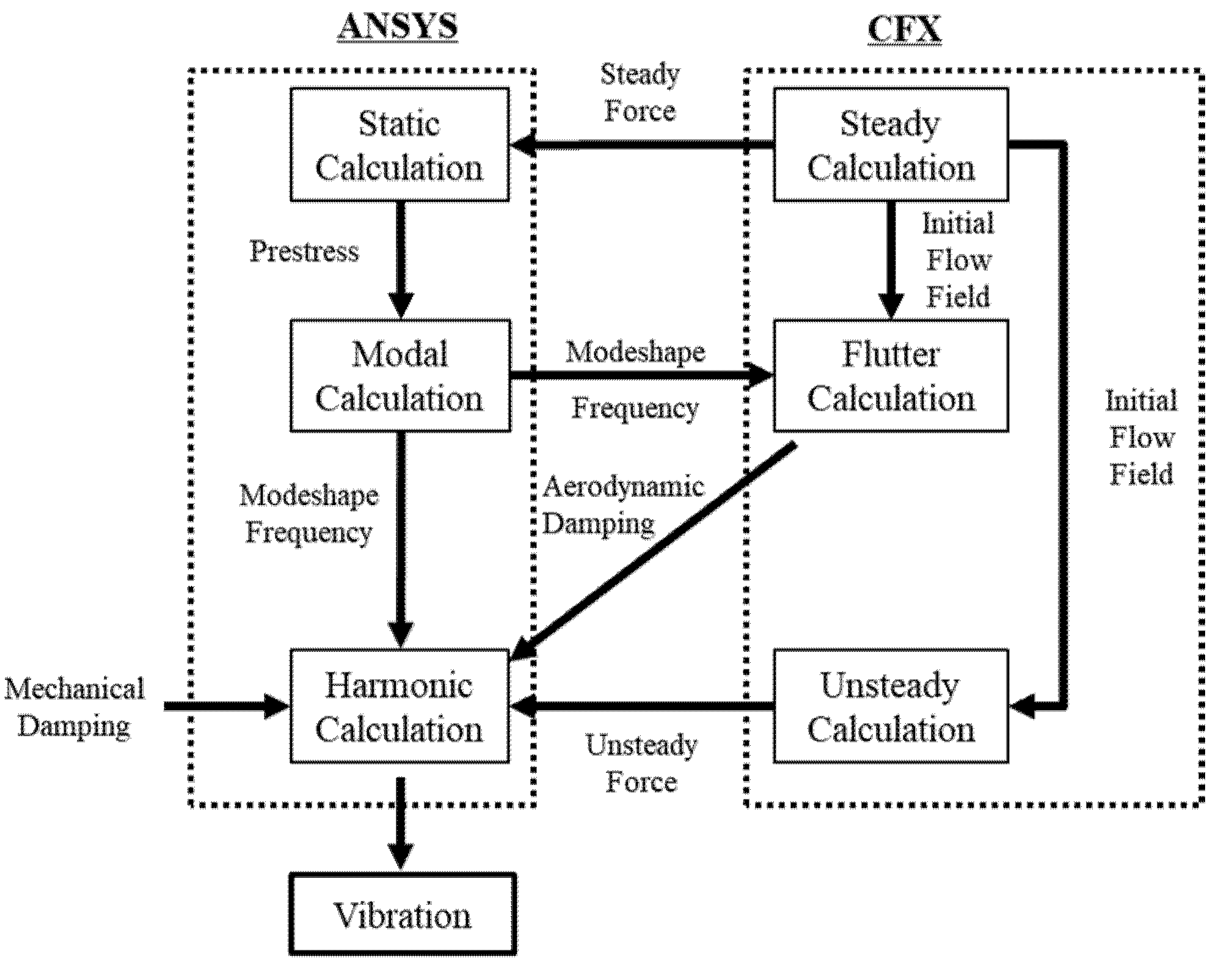
The forced vibration of the blade is calculated using the harmonic response on the basis of the mode superposition method. First, the modal calculation is used to provide the modal information of each order of the blade, including the mode shape and the natural frequency, for the subsequent calculation of the blade forced vibration. Second, the unsteady results of the blade surface pressure obtained after the unsteady flow field calculation are transformed into the frequency domain results at different frequencies by Fourier transform. Third, the aerodynamic damping of the blade is calculated by flutter, which is combined with mechanical damping to form the total damping. Finally, when calculating the blade vibration, the real and imaginary parts of the pressure in the frequency domain of the blade surface are loaded onto the finite element model under different excitation frequencies, and the harmonic response is calculated and solved to obtain the vibration results under the corresponding excitation frequencies.
The specific calculation process is shown in
Figure 3.
2.2. Fluid Domain
2.2.1. Solving Setup
The flow field is solved using CFX. A second-order backward Euler scheme is used for the temporal scheme, a high-resolution scheme is used for the spatial scheme, and a high-resolution scheme is used for the numerical accuracy of turbulence. The SST turbulence model is used to solve the problem.
The total pressure of the STRUTS is 101,325 Pa, the total temperature is 288.15 K, and the direction of intake is axial. The radial equilibrium equation is adopted as the outlet boundary condition. The solid surface adopts the adiabatic no-slip condition. Both sides of the fluid domain are set to rotating periodic interfaces. The stage model is used for the steady calculation, while the transient rotor–stator model is used for the unsteady calculation. The unsteady calculation takes the result of the steady calculation as the initial condition. The time step is 2.05761 × 10⁻⁶ s, that is, 360 physical time steps are required for R1 to sweep the complete computational domain. In the convergence condition, the flow rate and the force of the rotor blade have obvious periodic changes.
2.2.2. Method Verification
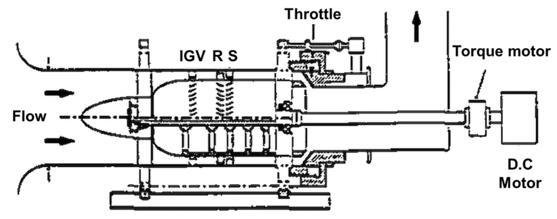
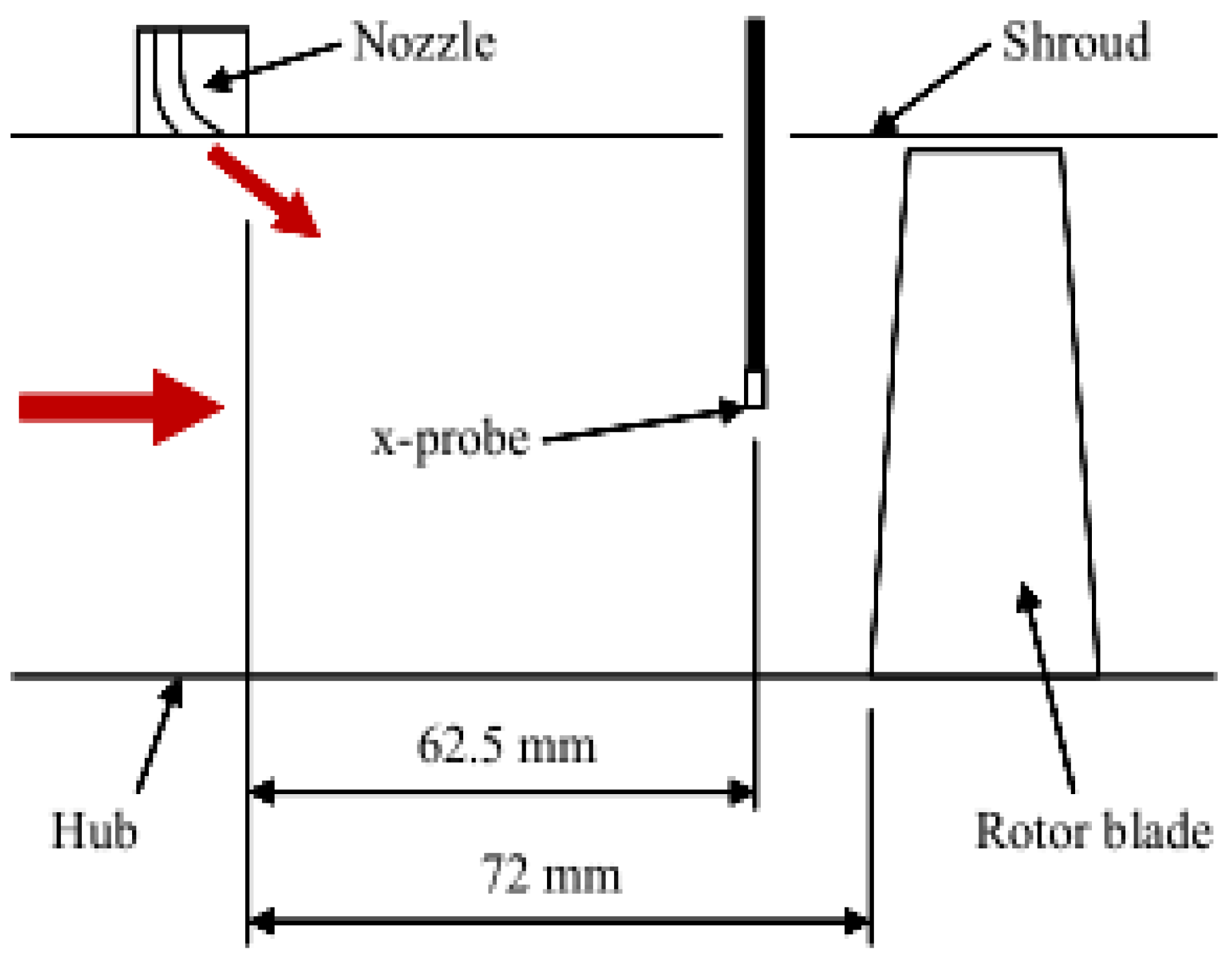
To verify the accuracy of the unsteady load prediction of compressor blades, the unsteady flow field of a compressor [
33,
34,
35] under near-design and high-load conditions is calculated. The compressor includes 60 inlet guide vanes, 58 rotor blades, and 60 stator blades, and the rotational speed is 1050 rpm, as shown in
Figure 4. The unsteady aerodynamic force at 50% stator blade span is measured by the pressure sensor. Andrew [
33] calculated the two-dimensional flow field and unsteady force.
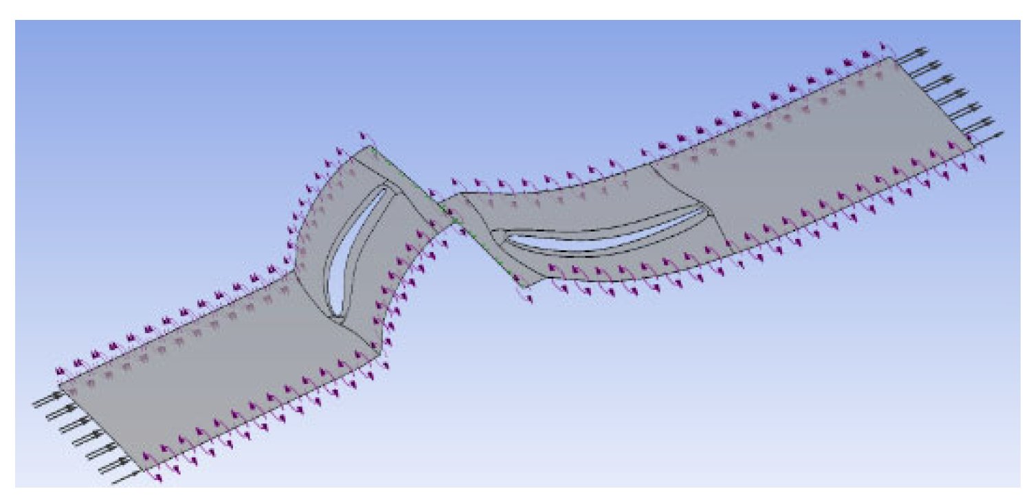
Only the rotor and stator blades were considered in the numerical simulation, and the number of stator blades was reduced to 58. Meanwhile, the stator blade profile was scaled to ensure that the axial distance and the cascade solidity are unchanged. The calculation domain is shown in
Figure 5.
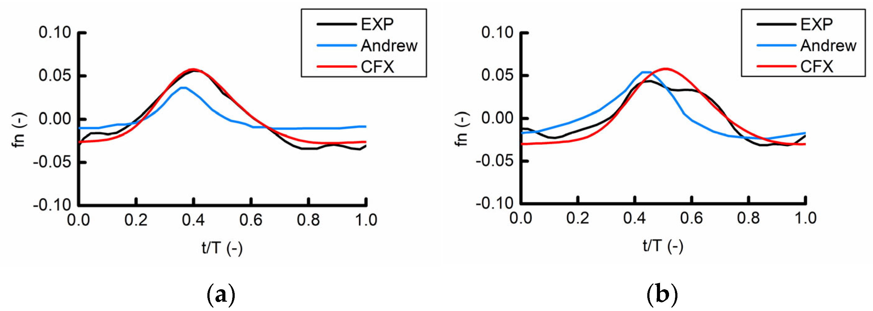
The calculated unsteady force is in good agreement with the experimental results, as shown in
Figure 6.
2.3. Structural Domain
2.3.1. Solving Setup
The structural calculation object is the R1 blade. The blade material is steel, with a density of 7850 kg/m3, a Young’s modulus of 200 GPa, and a Poisson’s ratio of 0.3. The commercial finite element software ANSYS is used for structural calculation. The R1 blade root constraint is the fixed support condition.
The aerodynamic damping of each mode is not calculated, but the total damping ratio of 0.001 is given for each mode.
2.3.2. Method Verification
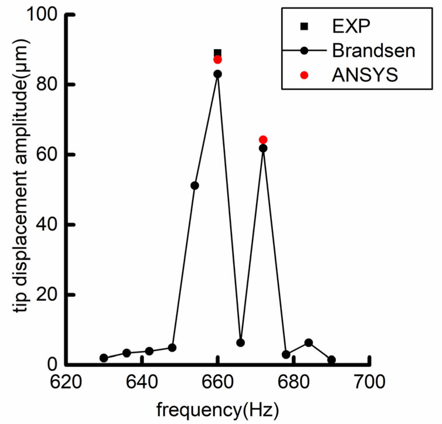
To verify the accuracy of the decoupling method in predicting the compressor blade vibration, the vibration of a compressor blade [
36,
37] excited by the pulsating jet hole is calculated in this paper, as shown in
Figure 7. In the references, the 660 Hz pulsating air flow of the jet hole excites the head rotor blade, which contains 15 jet holes and 43 rotor blades. The rotor blade is excited by the 660 Hz pulsating air flow and by the 720 Hz excitation caused by the rotor–stator interference between the jet hole and the rotor blade.
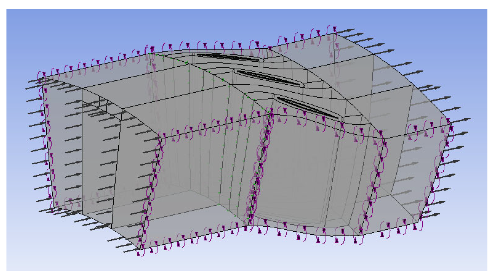
Brandsen [
37] carried out a bidirectional coupling calculation. To reduce the calculation cost, the numbers of jet holes and rotor blades were, respectively, changed to 14 and 42, and 1/14 channel was used for calculation without modifying the relevant geometry. At this time, the excitation frequency caused by the rotor–jet hole interaction was changed to 672 Hz. The calculation domain is shown in
Figure 8.
In this paper, the same numbers of jet holes and rotor blades are used for the decoupling calculation. The test results only show the amplitude of 660 Hz due to the change in the rotor interference frequency. The decoupling calculation results are in good agreement with the experimental and bidirectional coupling calculation results in the references, as shown in
Figure 9. The decoupling method can quickly and accurately predict the forced vibration of compressor blades.
2.4. Meshing and Verification
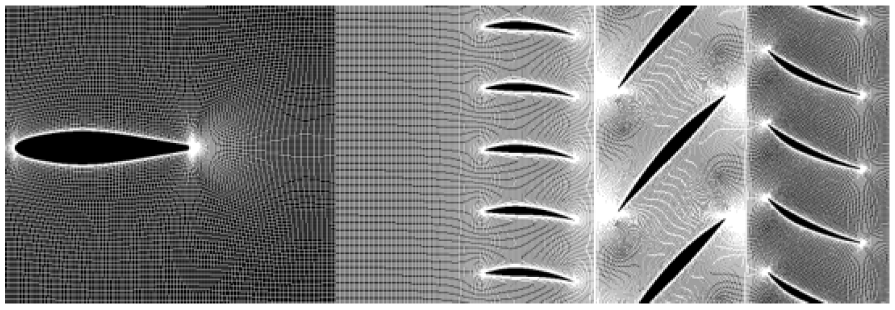
2.4.1. Meshing
NUMECA Autogrid5 was adopted for meshing. The mesh numbers of the STRUT, IGV, R1, and S1 channels are 1.08, 3.22, 4.37, and 3.41 million, respectively. The total number of mesh cells is 12.08 million, and the O4H mesh was adopted, as shown in
Figure 10. The tip clearance of R1 and S1 adopted a butterfly mesh with 17 mesh nodes in the radial direction.
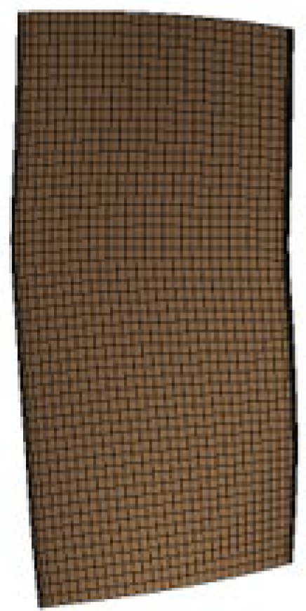
The finite element mesh type of the R1 blade is Solid186, which is a 20-node hexahedral element. The R1 blade has 40,230 mesh nodes. The mesh is shown in
Figure 11.
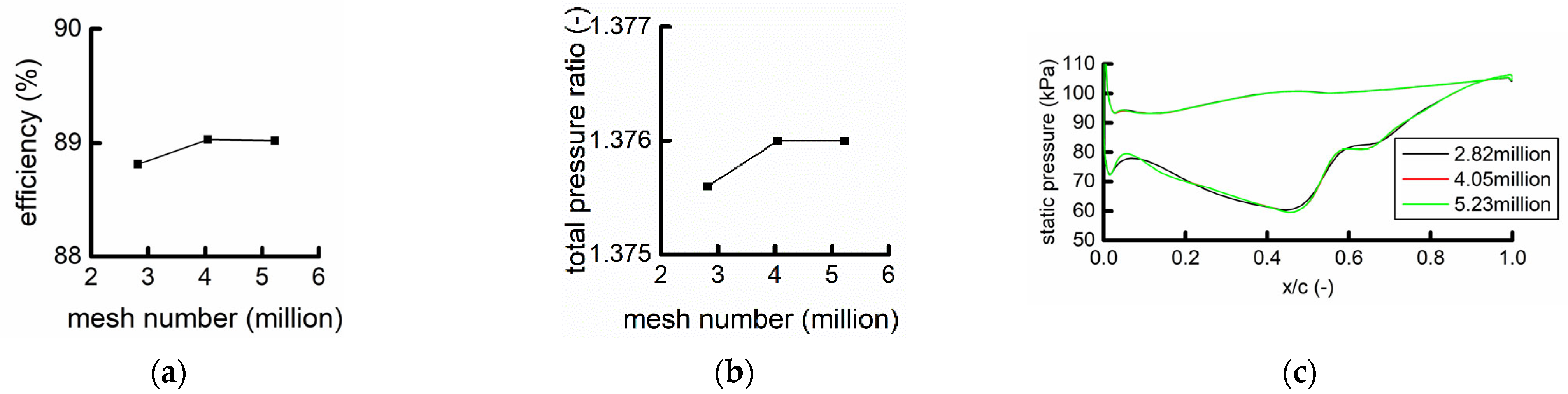
2.4.2. Independence
The convergence of the mesh in this paper was verified on other examples, including one IGV blade, one R1 blade, and one S1 blade without struts. The IGV, R1, and S1 blades are consistent with the examples in this paper.
Figure 12 shows that when the mesh number was 4.05 million, the efficiency, the total pressure ratio, and the pressure distribution did not change with the mesh number. Each channel mesh in this paper is consistent with the example.
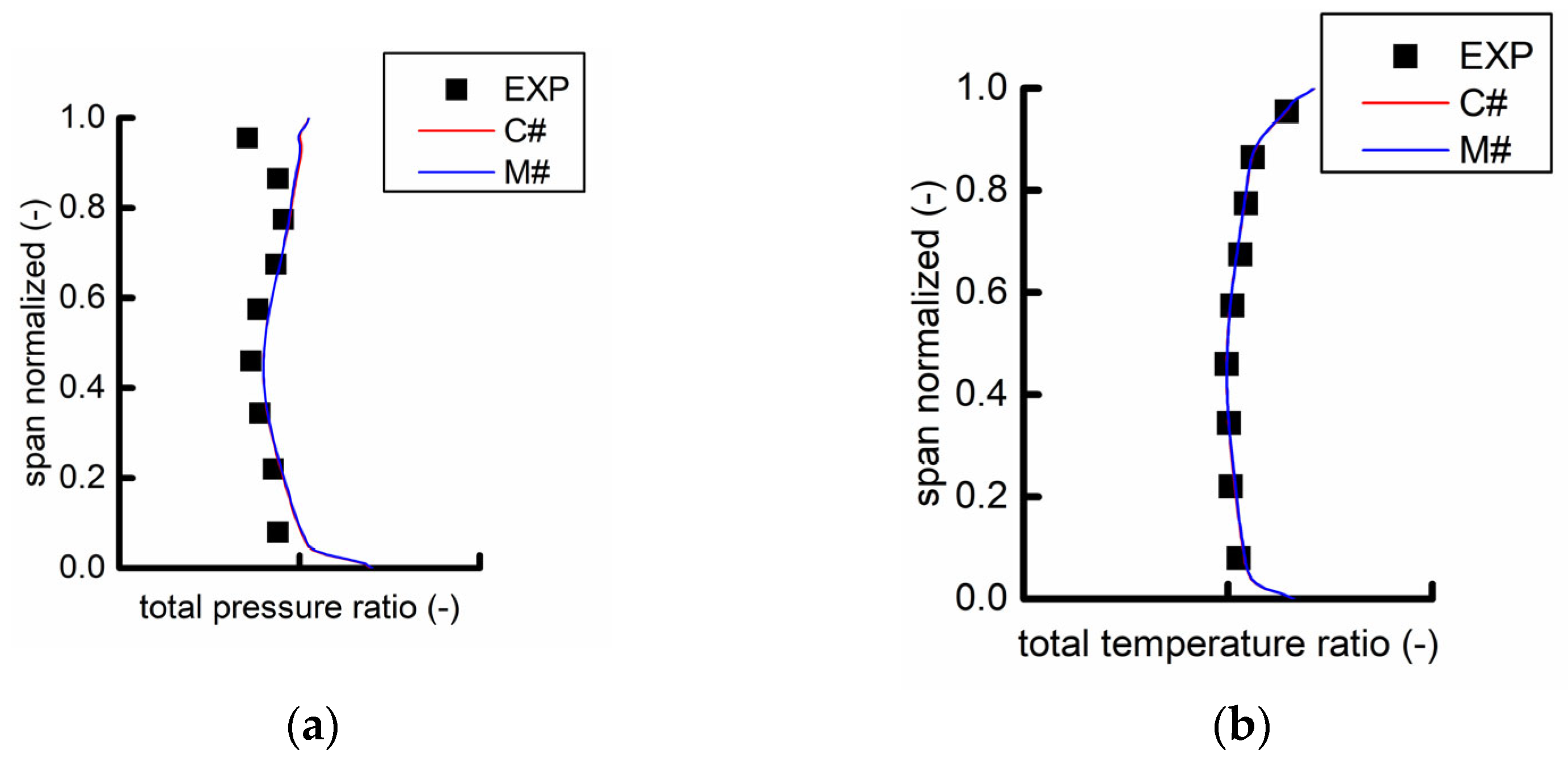
2.4.3. Test Data
The unsteady flow fields of the two examples were calculated. The static pressure at the outlet diameter of the flow field was adjusted to make the flow rate consistent with the test. The span distribution of the time-average values of the total pressure and the total temperature ratio of C# and M# were obtained and compared with the test results. The calculation and test results are shown in
Figure 13. The distributions of the total pressure ratio and the total temperature ratio obtained in the two examples are nearly the same, indicating that the position of the struts has little influence on the aerodynamic performance under design conditions. The calculated total pressure ratio and total temperature ratio are in good agreement with the test data.
3. Results and Discussion
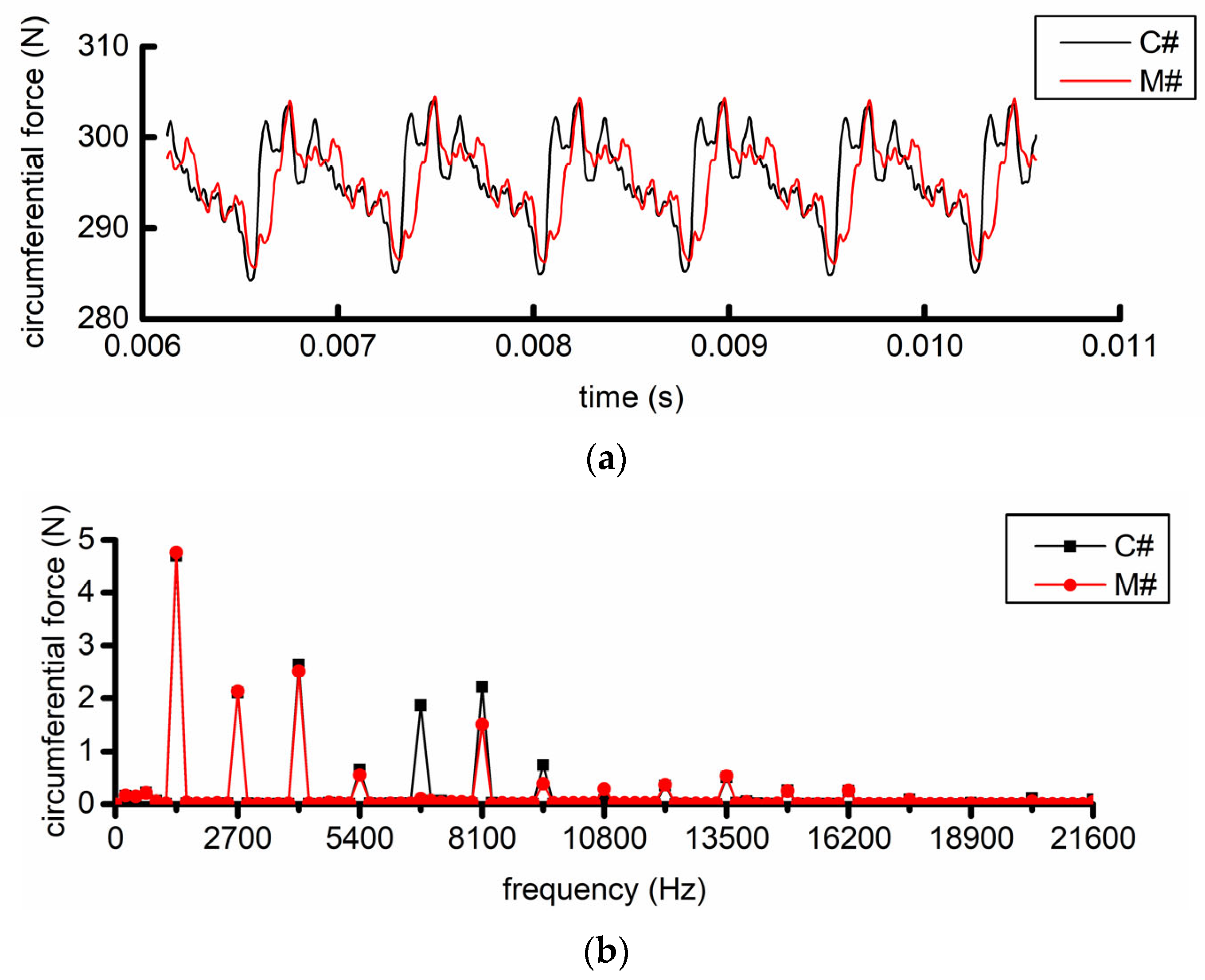
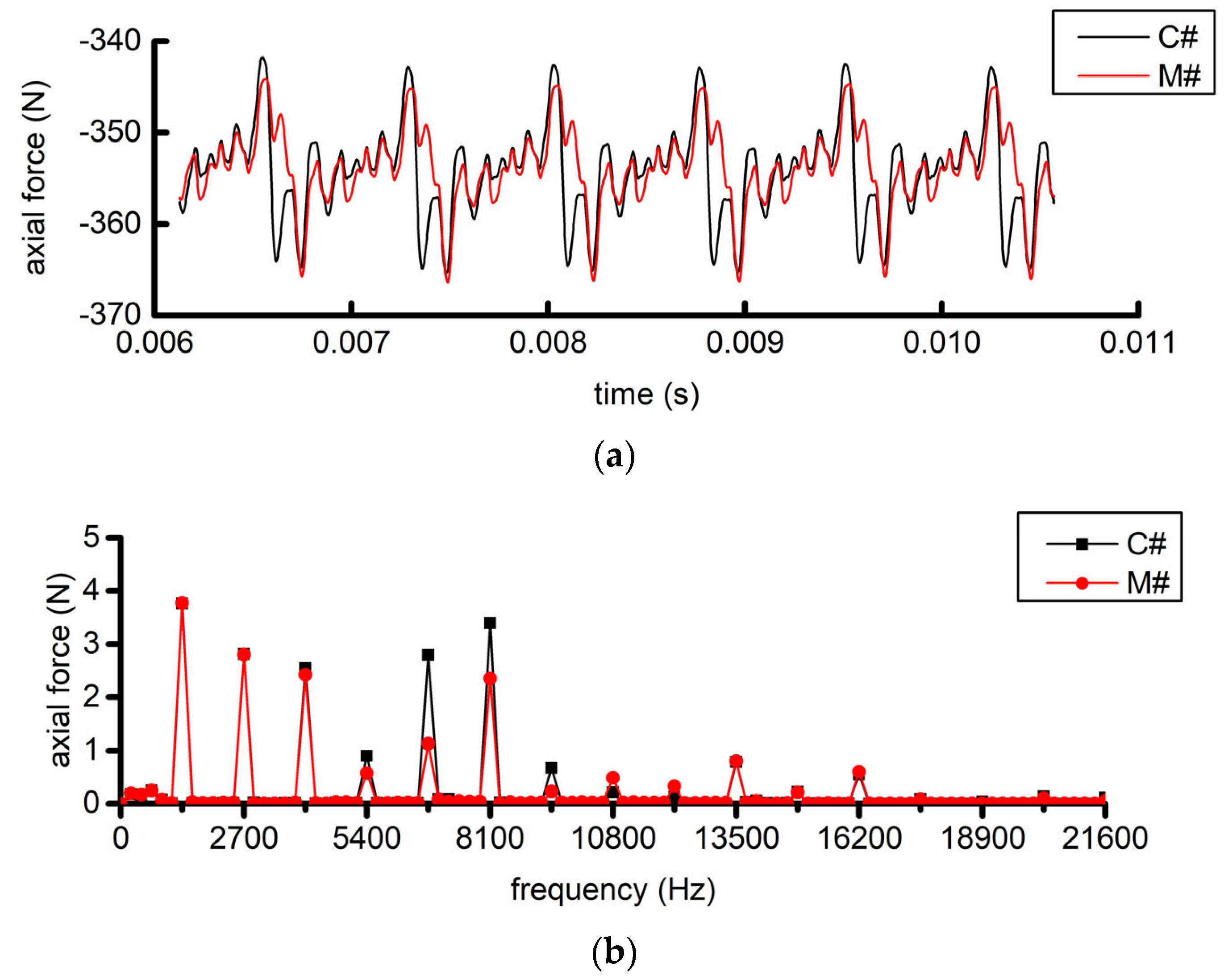
Figure 14 and
Figure 15 show the calculation results of the R1 blade forces. Fourier transform is applied on the time domain results to obtain the force components of the blades at different frequencies. The time domain results show that the R1 blade forces in the two examples show obvious periodic changes with time, and the calculation basically converges.
The results in the frequency domain indicate that the frequencies of each component under the force of R1 in the two calculation examples are mainly 1350 Hz and its frequency multiples., and the five frequencies with the largest amplitude are 1350, 2700, 4050, 6750, and 8100 Hz. These frequencies are directly related to the numbers of blades of STRUT, IGV, and S1 and the rotational frequency of R1. The above frequencies are 1, 2, 3, 5, and 6 times that of the struts excitation frequency, and 6750 and 8100 Hz are the fundamental frequencies of the S1 and IGV blades, respectively, as shown in
Table 1. These results indicate that R1 has many excitation sources, mainly including STRUT, IGV, and S1.
Notably, 6750 Hz (45EO) is not only the five-fold frequency of the IGV excitation but also the fundamental frequency of the S1 excitation, indicating that the load on R1 at this frequency is generated by the joint action of the struts and S1. Similarly, the 8100 Hz (54EO) load is affected by the struts and the IGV.
Figure 14b and
Figure 15b and
Table 2 show that the force components in the two directions of the struts have little difference. However, the axial and circumferential force components corresponding to the 5 and 6 octave frequencies of the struts, namely, the 1 octave frequencies of S1 and IGV, are significantly different, indicating that the position of the struts has a significant influence on the S1- and IGV-induced unsteady load.
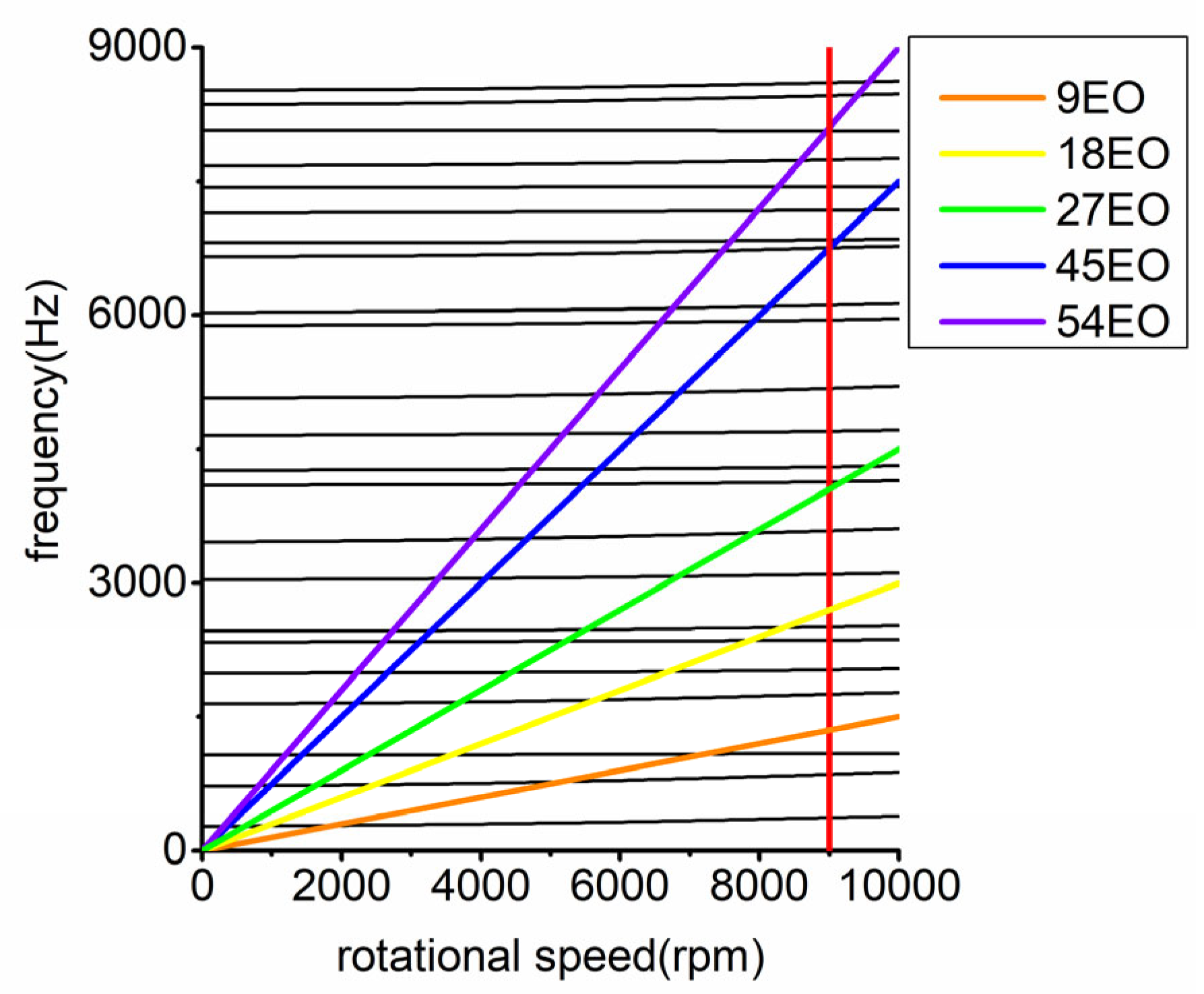
The natural frequencies of the first 23 modes under the stationary state and the design working condition of the R1 blade were taken, and the Campbell diagram was drawn according to the above main excitation frequencies, as shown in
Figure 16. Considering the C# and M# examples, the natural frequencies of every order mode of the average pressure were very small (less than 0.1 Hz), which could hardly be distinguished on the Campbell diagram. Therefore, only the Campbell diagram of the C# examples was drawn.
Figure 16 indicates that at the design speed of the example, the 54 EO excitation frequency is near the 21st mode natural frequency (8065.9 Hz), and the 45 EO excitation frequency is near the 16th mode natural frequency (6746.5 Hz).
The load at the 9, 18, 27, 45, and 54 EO frequencies subjected to R1 was used for harmonic response calculation to obtain the maximum amplitude of the R1 blade at the above excitation frequencies, as shown in
Table 3. The position of the struts has a significant influence on the vibration corresponding to the 1 octave frequency doubling of S1 and IGV, and the M# is 25.40% and 17.46% lower than C#.
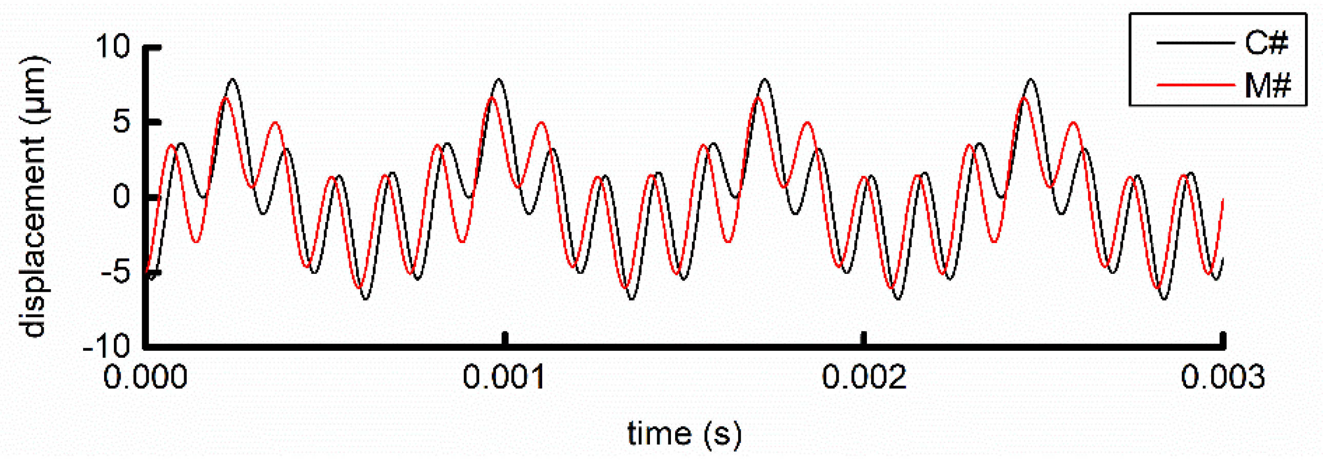
Taking the amplitude and phase of the blade tip at the above frequencies, the transient displacement response was reconstructed as shown in
Figure 17, where the tip response range of the C# example is 15.8% higher than that of the M# example.
3.1. Influence of Intake Strut Position on Unsteady Load and Vibration of Rotor Blade at IGV Fundamental Frequency (54EO)
The viscous wake of struts and IGV is one of the main excitation sources of the R1 blade. The total pressure deficit and nonuniform airflow angle caused by the wake leads to unsteady pressure waves propagating downstream on the surface of the R1 blade, forming the excitation to the R1 blade [
11,
29].
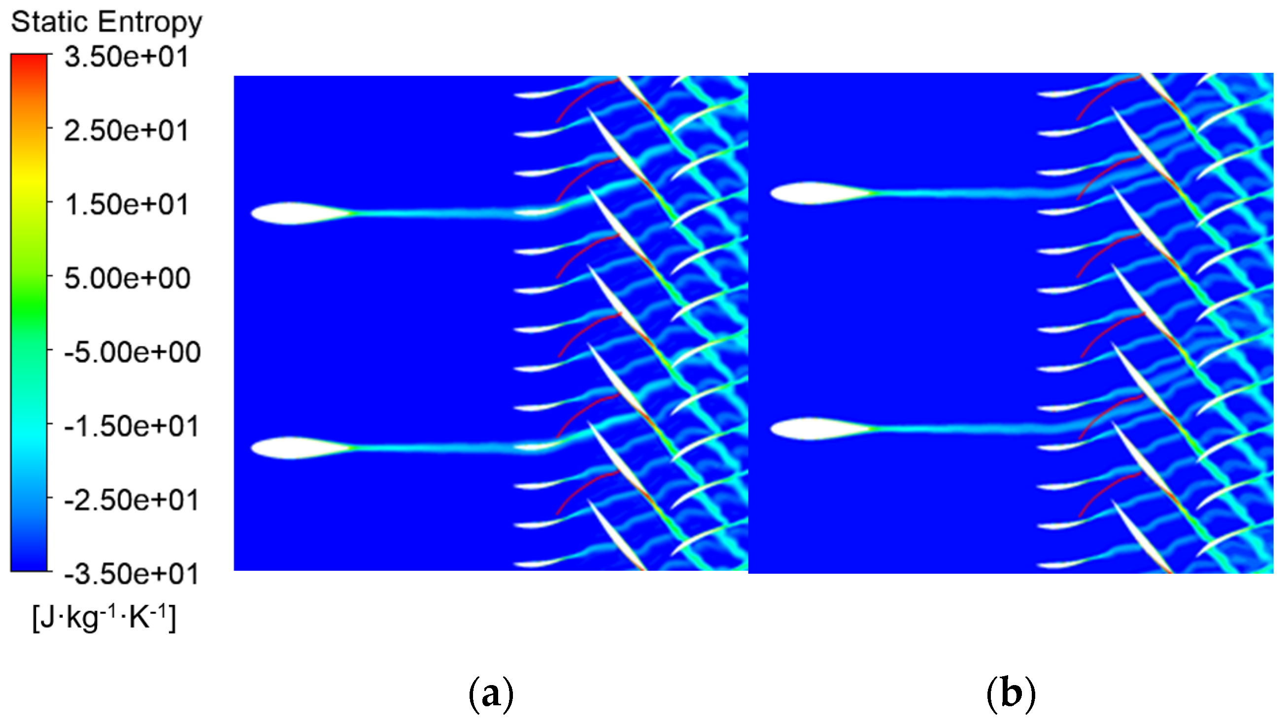
The static entropy in
Figure 18 shows that in the C# example, the struts wake is merged with the IGV wake at its corresponding position, and the width and strength of the merged wake are larger than those of the other IGV wakes. The width and entropy of the wake of the other IGVs in C# are largely unaffected by the struts. In the M# example, the struts wake is always between two adjacent IGV wakes, and no obvious difference exists between the wakes of each IGV.
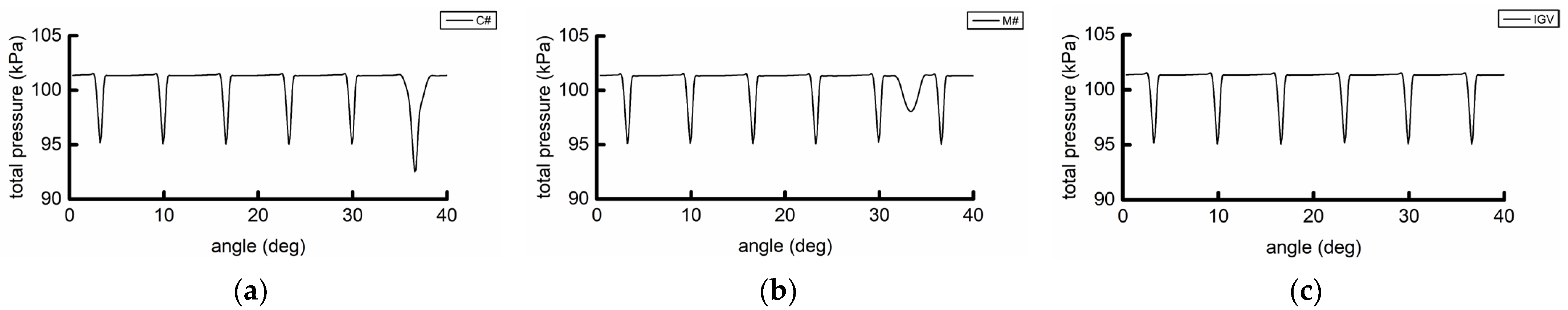
Figure 19 shows the circumfluence distribution of the time-average value of the total pressure at 50% of the span of the IGV/R1 interface, where ‘IGV’ is the reference value, representing the total pressure distribution solely caused by the IGV, which is drawn by directly copying the total pressure distribution from the left half to the right half. In the C# example, the total pressure deficit of 35–40° is wider and stronger than that of the other angles. In C# and M#, the total pressure distribution in the 1–32° and 35–40° ranges in M# are basically the same, indicating that the superimposed wakes of the struts and the IGV are stronger than those of the other IGV wakes, and the other IGV wakes are only slightly affected by the struts.
The spatial distribution of the total pressure is transformed into the temporal distribution according to the rotational speed, and the 54 EO component in the three cases can be obtained by spectrum analysis, as shown in the first three items in
Table 4. The total pressure amplitude of the M# example is 39.27% lower than that of the C# example.
The harmonic components of the two examples in the first two rows of
Table 4 are subtracted considering only the total pressure of the IGV, and the components (STRUT(C#) and STRUT(M#)) generated by different intake struts positions are obtained, as shown in the last two rows of
Table 4. The STRUT(C#) phase angle is 180.71° different from the STRUT(M#) phase angle, and the STRUT(C#) phase angle is only 1.87° different from the IGV component. The value of the single difference is consistent with the specific position of the struts in the two examples. In the two examples, the angle difference of the struts is half of the circumferential angle of the two IGV blades, which is equivalent to 180° at the 54 EO frequency. In the C# example, the phase angles of the total pressure components of the struts and the IGV are close, strengthening the total pressure amplitude. However, in the M# example, the phase angle difference is nearly 180°, resulting in the cancellation of the struts and IGV components. The angle difference indicates that the difference in the total pressure circumfluence component of IGV/R1 in the two examples is mainly due to the difference of the phase angle of the total pressure component of the struts that is directly caused by the change in the position of the struts, which affects the superposition of the struts and IGV components and further affects the inhomogeneous inlet conditions and the surface load of R1 blades.
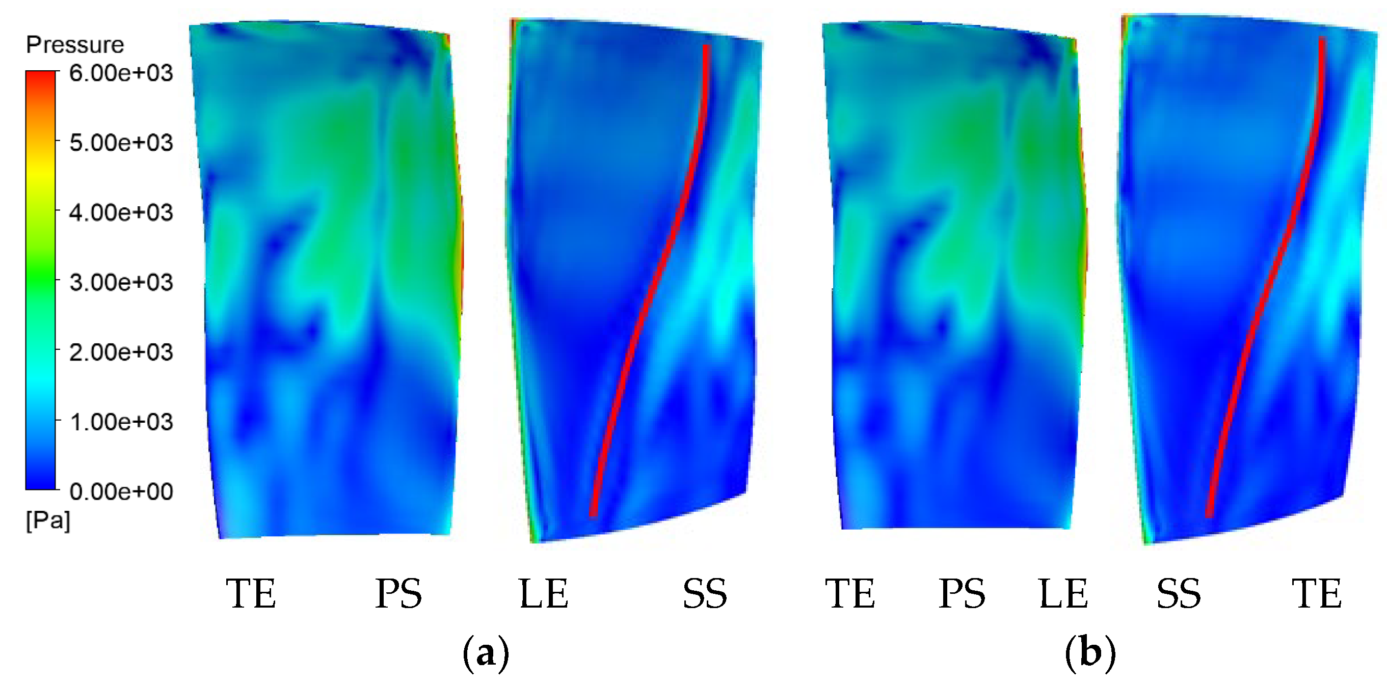
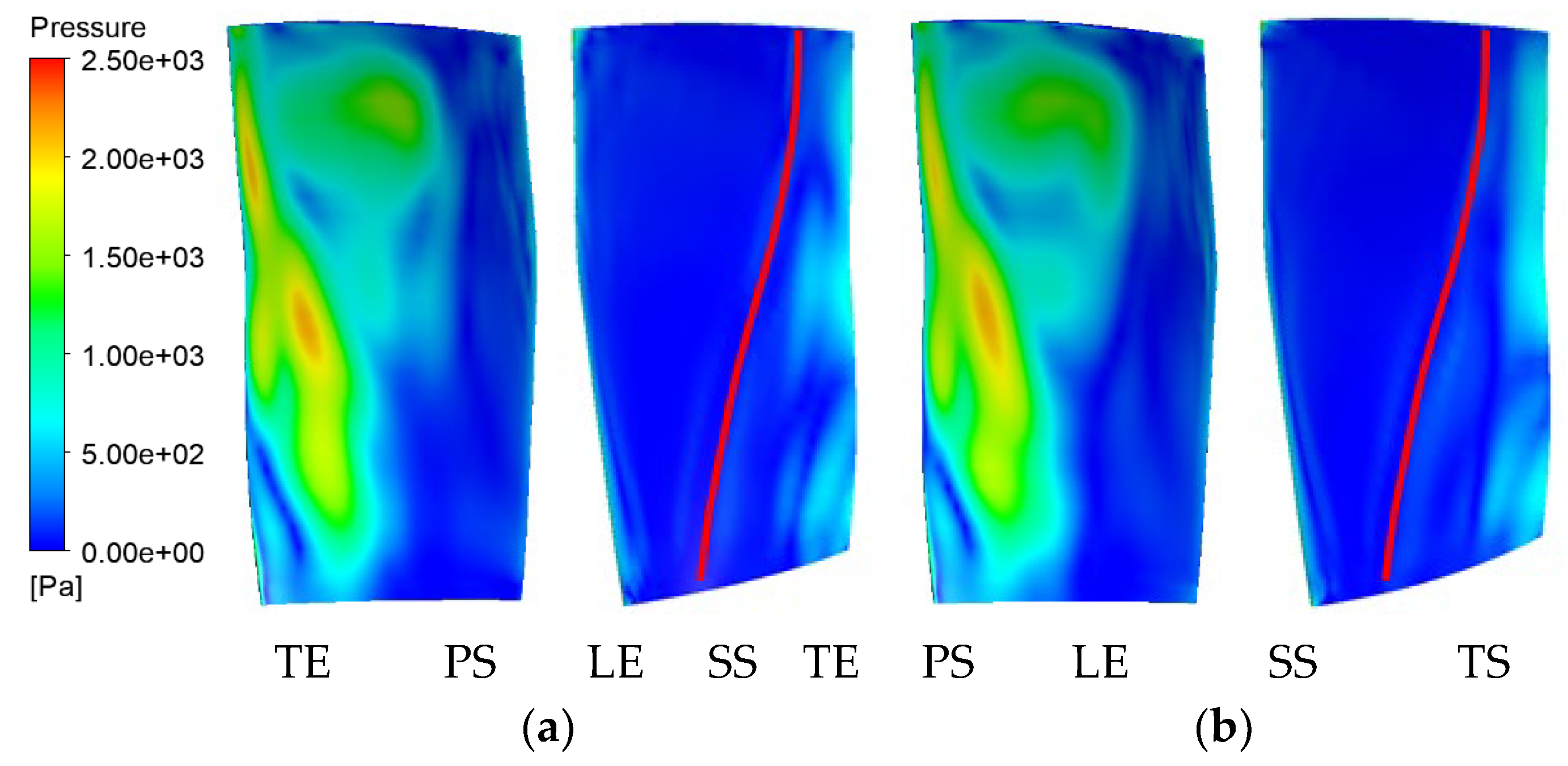
Figure 20 shows the 54 EO pressure amplitude of the R1 surface for two calculation examples. Among them, PS, SS, LE, and TE represent the pressure surface, suction surface, leading edge, and trailing edge of the blade, respectively.
Figure 20 indicates that the static pressure amplitude at 54 EO on the pressure surface is significantly higher than that on the suction surface. The unsteady pressure amplitude at 40–90% of the blade span on the pressure surface is large. The pressure amplitude of the pressure surface is the largest at the leading edge and decreases along the downstream direction. The pressure amplitude of the suction surface shows an opposite trend. The pressure wave is amplified after the shock wave, and the pressure amplitude behind the shock wave is obviously larger than that of the shock wave front. The pressure amplitude distributions of the two examples are basically the same, indicating that the position of the struts has little influence on the propagation of the unsteady load distribution at the IGV fundamental frequency on the surface of the R1 blade.
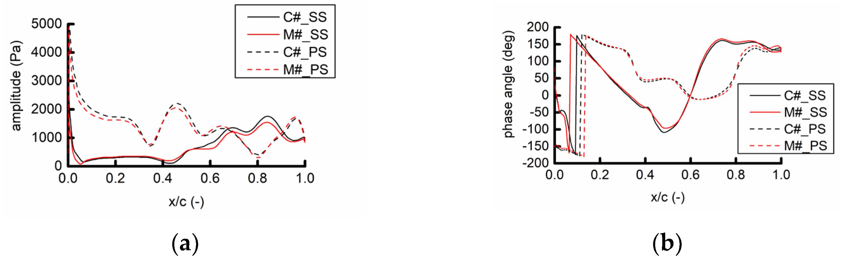
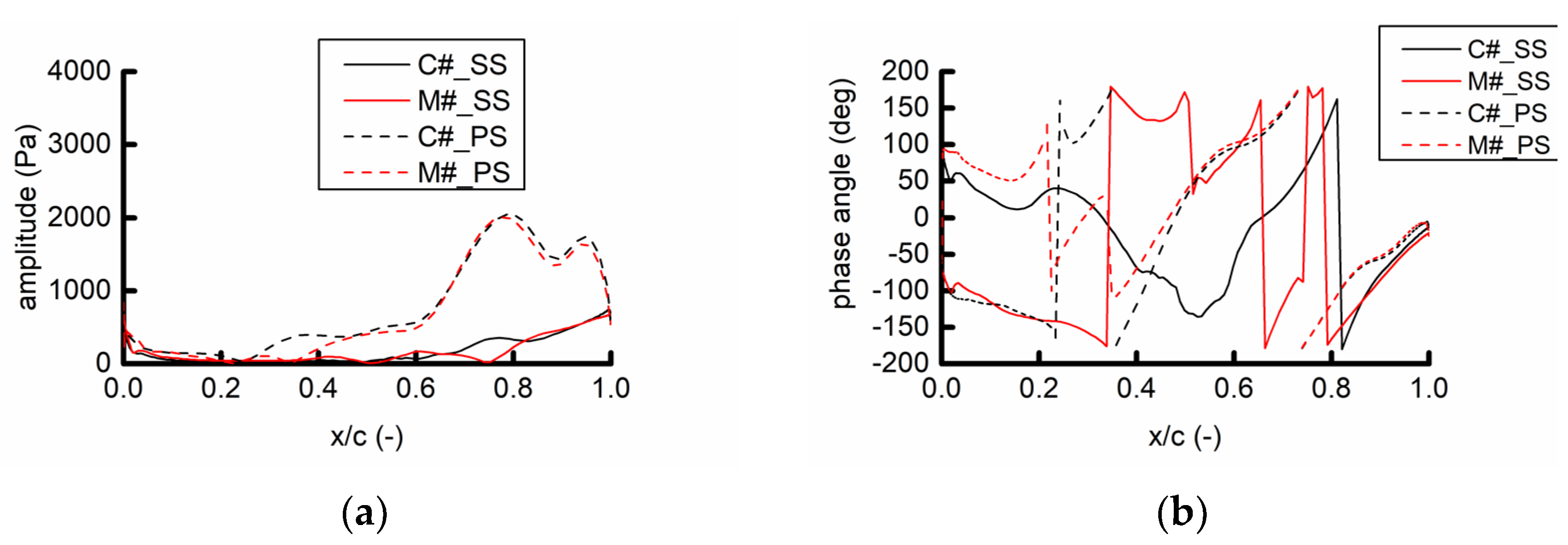
Figure 21 shows the amplitude and phase angle of the 54 EO pressure on the suction surface and the pressure surface at the 50% blade span. Overall, the pressure amplitude in the C# example is larger than that in the M# example, but the spatial distribution of the two is similar, and the pressure amplitude near the leading edge is higher than those in the other choroidal positions. The phase angle distribution of the two is basically the same, indicating that the pressure waves caused by the struts and the IGV move downstream at the same time, and the propagation process of the pressure wave is basically the same.
Figure 22 compares the pressure amplitude and phase angle of 54 EO on the suction and pressure surfaces at the 80% blade span. Overall, the pressure amplitude in the C# example is slightly larger than that in the M# example, but the distribution of the two is similar, and the phase angle distribution is basically the same. This result indicates that the influence of the position of the struts on the unsteady leaf surface at the IGV frequency has a similar rule at different blade spans.
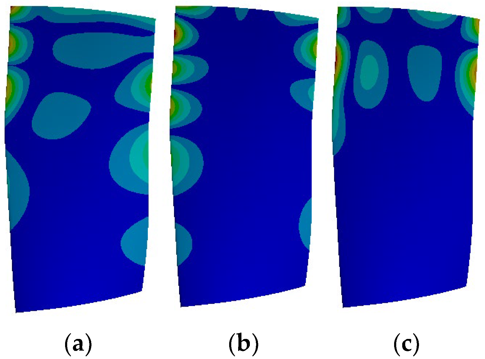
According to the Campbell diagram in
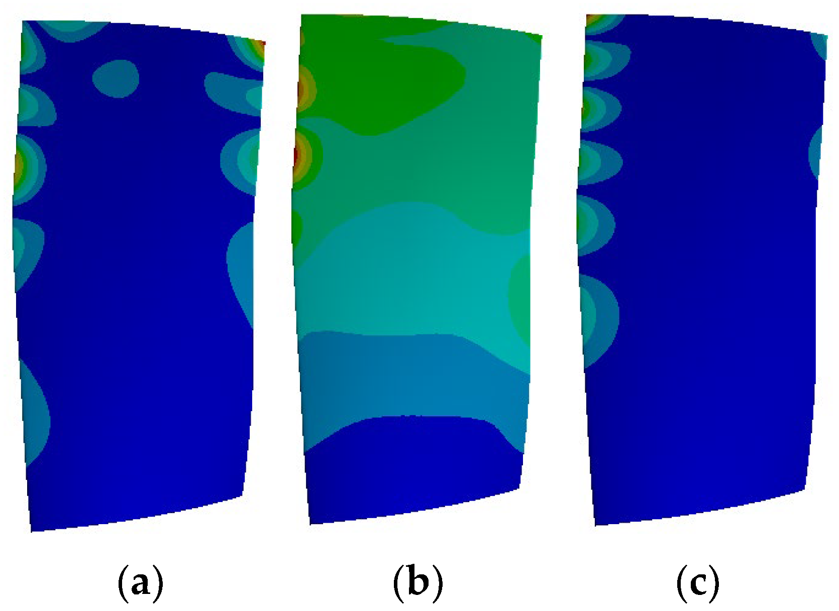
Figure 16, the 54 EO excitation frequency is near the natural frequency of Mode 21 (8065.9 Hz), which is between Modes 20 and 22. The three modes are shown in
Figure 23.
Figure 24 shows the 54 EO frequency amplitudes of the R1 blades in the C# and M# examples. The amplitude distribution of the two examples is similar, showing a large amplitude at the anterior trailing edge and near the tip of the blade and a small amplitude at the middle and root of the blade, which is much different from the mode shape of the 21st order. This is because although the excitation frequency is closest to the natural frequency of Mode 21, the displacement direction of Mode 21 is mainly radial, while the pressure load is the normal load on the blade surface, and this mode is not sensitive to the pressure load. In the 20th and 22nd mode shapes, the vibration displacement direction is similar to the normal direction of the blade surface, which is sensitive to the pressure load. The 54 EO vibration of the blade is mainly composed of the superposition of the 20th and 22nd modes. The unsteady load of the blade is changed by the change in the position of the struts. Inconsequently, the overall amplitude of C# is slightly larger than that of M# but has little influence on the specific distribution of the amplitude of the R1 blade surface.
3.2. Influence of Intake Strut Position on Unsteady Load and Vibration of Rotor Blade at S1 Fundamental Frequency (45 EO)
The circumferential nonuniform potential flow field is caused by the S1 in the downstream of R1, leading to the change in the load on the R1 blade surface, which belongs to potential flow interference [
11,
29].
Figure 25 shows that the distribution of the pressure amplitudes of C# and M# is similar, and the amplitudes of the pressure and suction surfaces near the downstream position are significantly larger than those in the front position. On the one hand, the area near the trailing edge of the R1 blade is near the leading edge of the S1 blade, and the pressure surface faces the leading edge of the S1 blade. Therefore, the area near the trailing edge (especially the trailing edge of the pressure surface) is strongly disturbed by the downstream S1 potential flow. On the other hand, on the suction surface, the potential flow disturbance from the downstream S1 stator blade has difficulty passing through the shock wave and continues to propagate upstream, so the wave-front position of the suction surface is mainly affected by the upstream struts and IGV.
In
Figure 25, the pressure amplitude distribution at the 40–90% blade span behind the suction surface shock wave is significantly different between the two calculation examples. To analyze the reasons,
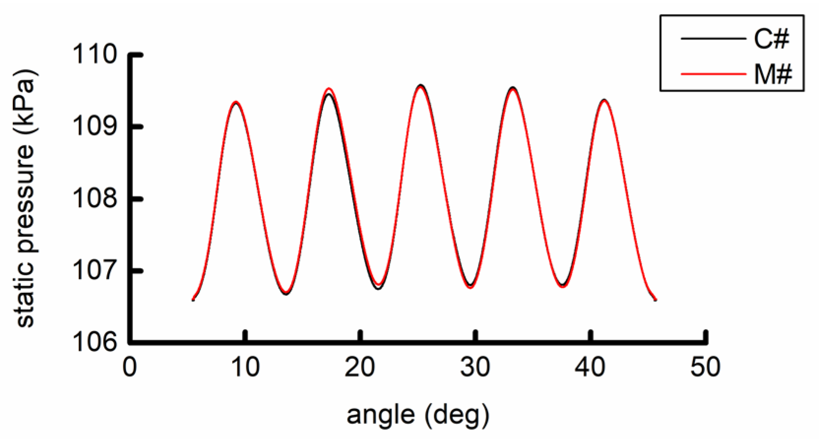
Figure 26 shows the distribution of the time-average value under static pressure at the 50% blade span on the R1/S1 interface, which reflects the influence of the potential flow propagating upstream from the downstream S1 blade. In the two examples, the circumferential distribution of the time-average value under static pressure is basically the same, and the change in the position of the struts does not significantly change the circumferential nonuniform pressure field caused by the S1 blades. This phenomenon indicates that the circumferential position of struts has little influence on the upward propagation potential flow of S1, and the difference in the unsteady load on the blade surface may be mainly caused by the superposition relationship between the influence of the upstream struts and the downstream stator blades.
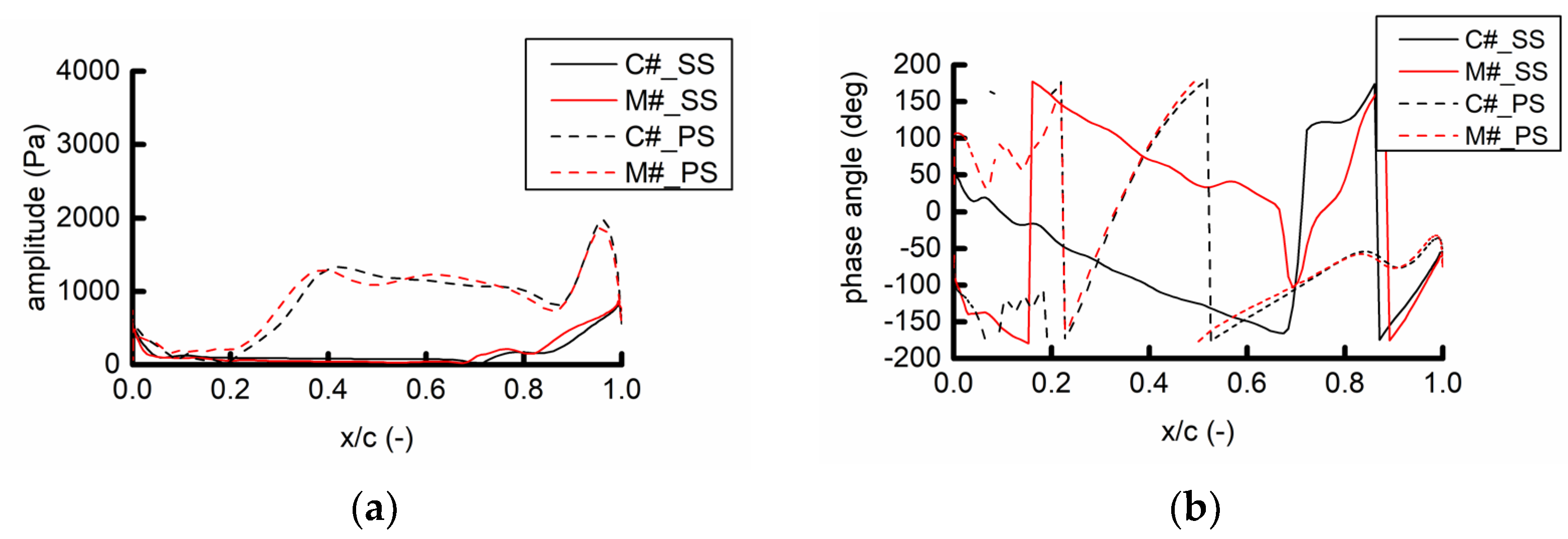
The chordwise distribution of the pressure amplitude in
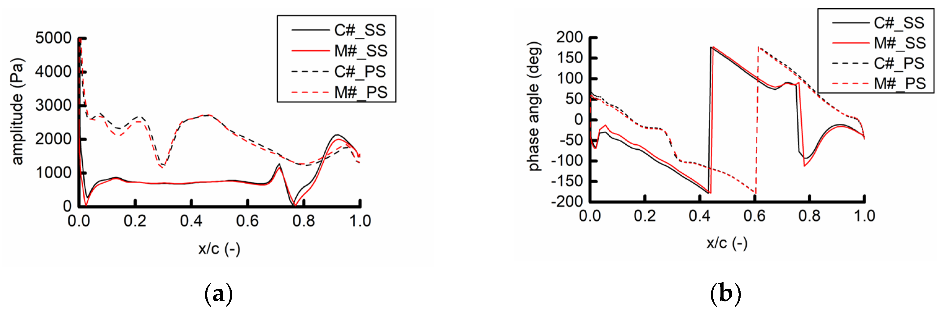
Figure 27 shows that the pressure amplitude on the pressure surface is larger than that on the suction surface, and the pressure amplitude near the trailing edge is obviously about the leading edge, indicating that at 45 EO, the influence of the downstream S1 potential flow interference is significantly stronger than that of the upstream struts. At the 30–50% chord length on the pressure surface and 70–80% chord length on the suction surface, the pressure amplitudes of the two examples are obviously different, and the phase angle difference changes from approximately 150° to near 0°, indicating that the influence of the upstream struts and downstream potential flows at these two locations is similar. At its upstream, the pressure amplitude is generally small, and the phase angle decreases with the chord length, indicating that the pressure wave propagates downstream. Overall, the pressure phase angles of the two examples have an approximately 150° difference, which corresponds to the position of the struts in the two examples, indicating that the influence of the upstream struts is dominant here. At its downstream, the pressure amplitudes of the two examples are similar, and the phase angles increase with the chord length and are similar, indicating that the pressure waves in the two examples nearly propagate upstream at the same time, which corresponds to the constant position of the S1 blade in the two examples, indicating that the potential flow influence of the S1 blade at this point is dominant. These conditions indicate that the loads on the leading and trailing edges of the R1 blade are dominated by the upstream strut’s wake and the downstream S1 potential flow field, respectively, while the middle chord of the R1 blade is affected by the superposition of struts and S1.
Figure 28 shows that the pressure amplitude and phase angle at 80% spanwise of the two examples are similar at the leading and trailing edge, while the position in the middle chord length of the pressure surface and after 70% chord length of the suction surface (shock wave) are different due to the different positions of the struts. It also shows that the unsteady load at different leaf heights is affected by the superposition of struts and S1 and are related to the circumferential position of the struts.
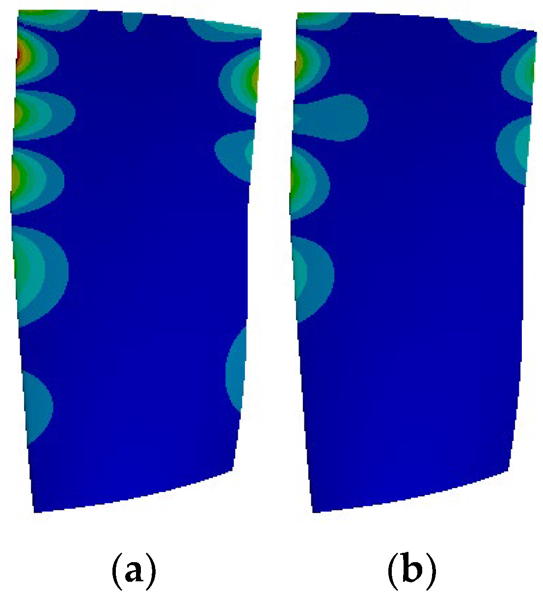
According to the Campbell diagram in
Figure 16, the 45 EO excitation frequency is near the natural frequency of Mode 16 (6746.5 Hz), which is between Modes 15 and 16. The three modes are shown in
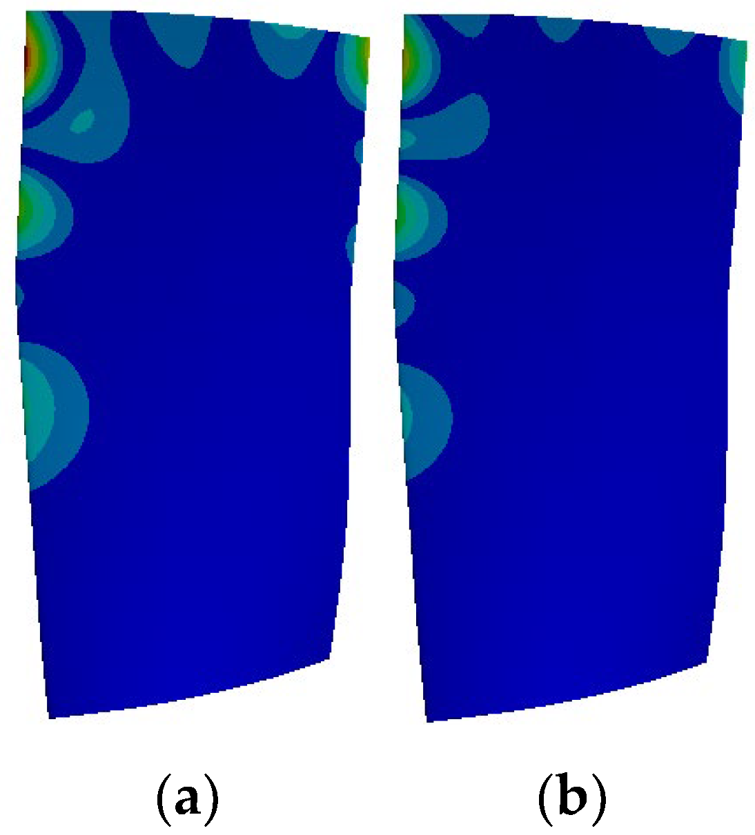
Figure 29.
Figure 30 shows that the 45 EO frequency amplitude distribution of the R1 blade in the C# and M# calculation examples is similar, and its 16th mode shape is similar, indicating that the 16th mode near this frequency plays a dominant role in vibration. The position of struts and the change in the load caused by struts do not change the distribution of the blade vibration displacement obviously.
Notably, the R1 for the twisted blade, blade, and shock wave positions is different at different blade spans, while the upstream downstream S1 blade affects the direction of propagation of the plate. These factors result in the different superposition relationships of the influences of struts and IGV at different blade spans, resulting in a difference in the pressure amplitude distribution at the 40–90% blade span after the shock wave on the R1 blade suction surface in
Figure 25.


