Article

Vibration Analysis of Two-Stage Helical Gear Transmission with Cracked Fault Based on an Improved Mesh Stiffness Model

National Key Laboratory of Vehicular Transmission, Beijing Institute of Technology, Beijing 100081, China
*
Author to whom correspondence should be addressed.
Machines 2022, 10(11), 1052; https://doi.org/10.3390/machines10111052
Submission received: 11 October 2022 / Revised: 3 November 2022 / Accepted: 6 November 2022 / Published: 9 November 2022
(This article belongs to the Section Machines Testing and Maintenance)

Abstract

:
The crack fault has an important influence on the vibration characteristics of the transmission system. This paper is devoted to analyzing fault mechanism and dynamic characteristics of transmission with gear crack, which provides the basis for crack diagnosis and monitoring of helical gear in two-stage transmission system. For this purpose, an improved calculation method of time-varying meshing stiffness with crack fault is proposed considering the axial force of the helical gear. The influence of crack depths and angles on stiffness is analyzed. Based on this, the dynamic model of the two-stage helical gear transmission system is established using the lumped mass method. The influence of crack parameters on the characteristics of the transmission system is studied. In order to better diagnose the crack fault of the helical gear, the statistical index in time domain is calculated and the sensitivity to crack fault is analyzed. It is shown that the stiffness decreases by 25%, and the vibration acceleration increases by 8.3% after the axial force component is considered into the stiffness of the crack gear pair. The meshing stiffness decreases with the increase of crack depths and crack angles. The dynamic model is verified by rig test. Periodic impact exists in the system. The time of entering meshing of the cracked tooth and the time of complete disengagement is observed in the residual signal. In the frequency domain, there appear sidebands on the mesh frequency of the first gear pairs and its harmonics, the second gear mesh frequency and its harmonic frequencies. There is a little influence on the vibration acceleration of the driven gear of the second-stage. According to the signals in the frequency domain and the time domain, we can tell at which stage the gear is cracked. While through the time required for the crack tooth from engagement to disengagement completely, we can tell which gear is cracked. The sensitivity of skewness, impulse factor and kurtosis to crack fault decreases successively. The results provide theoretical basis for crack fault diagnosis of a two-stage helical gear transmission system.

1. Introduction

A helical gear transmission system has the characteristics of smooth transmission, strong bearing capacity and high speed. It has been widely used in aerospace, ships, automobile transportation and other fields. It is shown that gear faults account for 60% of the transmission faults [1]. Driven by motor directly, the gear working in the transmission system of pure electric vehicle bears high-frequency alternating load, which is prone to crack failure. Analysis of the vibration characteristics of cracked gear provides a theoretical basis for the diagnosis of crack fault. The accurate calculation of time-varying meshing stiffness is the key to dynamics analysis. Therefore, the calculation of helical gear meshing stiffness accurately with axial force is considered important. The influence of a crack on the vibration characteristics of a two-stage helical gear transmission system is of great significance to the fault diagnosis of helical gear.
There are several methods to calculate the stiffness of helical gears. The finite method is more accurate, but refined by the mesh accuracy, the calculation speed is relatively slow. In some systems [2], using the analytical Hertzian model for contact deformation and FEA simulation for the bending and foundational deflection to get a more accurate stiffness in dynamic model. The analytic-FE method combines the analysis method and the finite method more accurately and saves time, but it is slightly complex for some dynamic model. The analytical method is simplified, with a lower accuracy, but it is fast. The calculation of the gear stiffness using potential energy method was proposed first by Yang and Lin [3]. In the method, the gear considered was a cantilever beam with variable cross-section. The elastic deformation of the gear included Hertz contact energy, bending deformation energy and axial compression energy. The shear deformation was also considered by Tian [4]. The foundation deformation formula was derived by Sainsot [5] and the deformation was included in the calculation of gear stiffness. In the above assumptions, the cantilever beam was from the base circle. When the root circle of the gear was larger than the radius of the base circle, the energy and deformation between the root circle and the base circle was ignored. To solve this problem, the stiffness calculation formula with a different radius of root circle and base circle was derived [6]. The error of meshing stiffness of gears with different number of teeth was reduced compared with the finite element calculation result. A cantilever beam model starting from the root circle was proposed by Ma [7] of Northeastern University. The accurate transfer curve between the tooth profile and the root circle was studied rather than considering the size relationship between the root circle and the radius of the base circle. Compared with the previous method, the calculated stiffness is closer to the finite element calculation result. After that, an improved calculation method for the helical gear was proposed [8]. With the action of axial force considered, the meshing stiffness of the helical gear was calculated [9,10,11,12]. Yan [13] calculated the meshing stiffness of the helical gear using the connection of the contact line method and the slice method. Zhang [14] calculated the meshing stiffness of helical gears using the FE-analytical slice method. Yang [15] improved the stiffness calculation of helical gears considering the flexible deflection and the clearance. Huangfu [16,17] improved the stiffness calculation method of helical gear and calculated the stiffness of helical gear with a space crack. Lin [18] studied the meshing stiffness of helical gears with crack faults.
The gear transmission system mainly consists of gears, bearings and shafts. The gear transmission system was regarded as a single degree of freedom system. Based on the impact theory, the excitation generated by the meshing impact was calculated. It was not until 1950s that the gear meshing transmission model was equivalent to the spring-mass model [19] for the first time. The one DOF model of pure torsion was established. In 1991, Kahraman and Singh [20] established a 3 DOF model considering the coupling multi-degree-of-freedom model and studied the influence of tooth clearance on it. Brethee [21] established an 8 DOF model considering the influence of motor, load and bearing. Chen [22] established the dynamics model of high-speed locomotive vehicle and gear transmission with crack faults.
Meng [23] established a dynamic model with the first-level spur gear cracked. The vibration response of the crack failure was analyzed by segmental stiffness method. Chen [24] developed the dynamic model and analyzed dynamic characteristics of a two-stage planetary gear transmission with cracked gear. The oil lubrication of bearing is analyzed in the literature [25]. An accurate dynamical model of gear systems was established [26]. Considering the eccentricity, Esayed [27] established modified helical gear models. A lumped element model was developed considering meshing stiffness and backlash [28]. Wang [29] established a distributed helical gear dynamic model with error tooth profiles. Yan [30] achieved tooth surface optimization by analyzing the dynamic characteristics of helical gears. Jiang [31] studied the helical gear dynamics model considering the friction. Wei [32] studied the calculation of time-varying meshing stiffness and dynamic characteristics of a two-stage helical gear system based on potential energy method. Liu [33] used the energy method to calculate the meshing stiffness and developed a 16 DOF model of gear-bearing-rotor using the lumped mass method.
The existing literature mainly focuses on spur gear cracks and planetary gear cracks. However, there are a few studies on the dynamics of a two-stage helical gear transmission system with crack failure considering axial force. In this paper, a calculation method of meshing stiffness of helical gear with crack fault considering the axial force and the crack fault is proposed. The lumped mass model of a two-stage helical gear transmission system with gear cracked is established. The influence of time-varying mesh stiffness and transmission error on the dynamic characteristic of gears is studied. The time-frequency signal of vibration acceleration of helical gear is obtained and compared with the experimental results. The influence of crack parameters of helical gear on vibration characteristics of the two-stage transmission system is analyzed. Considering the axial force in the stiffness model, the impact amplitude of the cracked gear vibration acceleration is 25% larger. This is helpful to realize the diagnosis of crack fault. There appears sidebands around the first mesh frequency and the second mesh frequency and their harmonics. However, the amplitude of vibration acceleration of driven gear on the output shaft changes a little when the driving gear on the input shaft is cracked.

2. Calculation of Time-Varying Meshing Stiffness of Helical Gears with Crack Fault

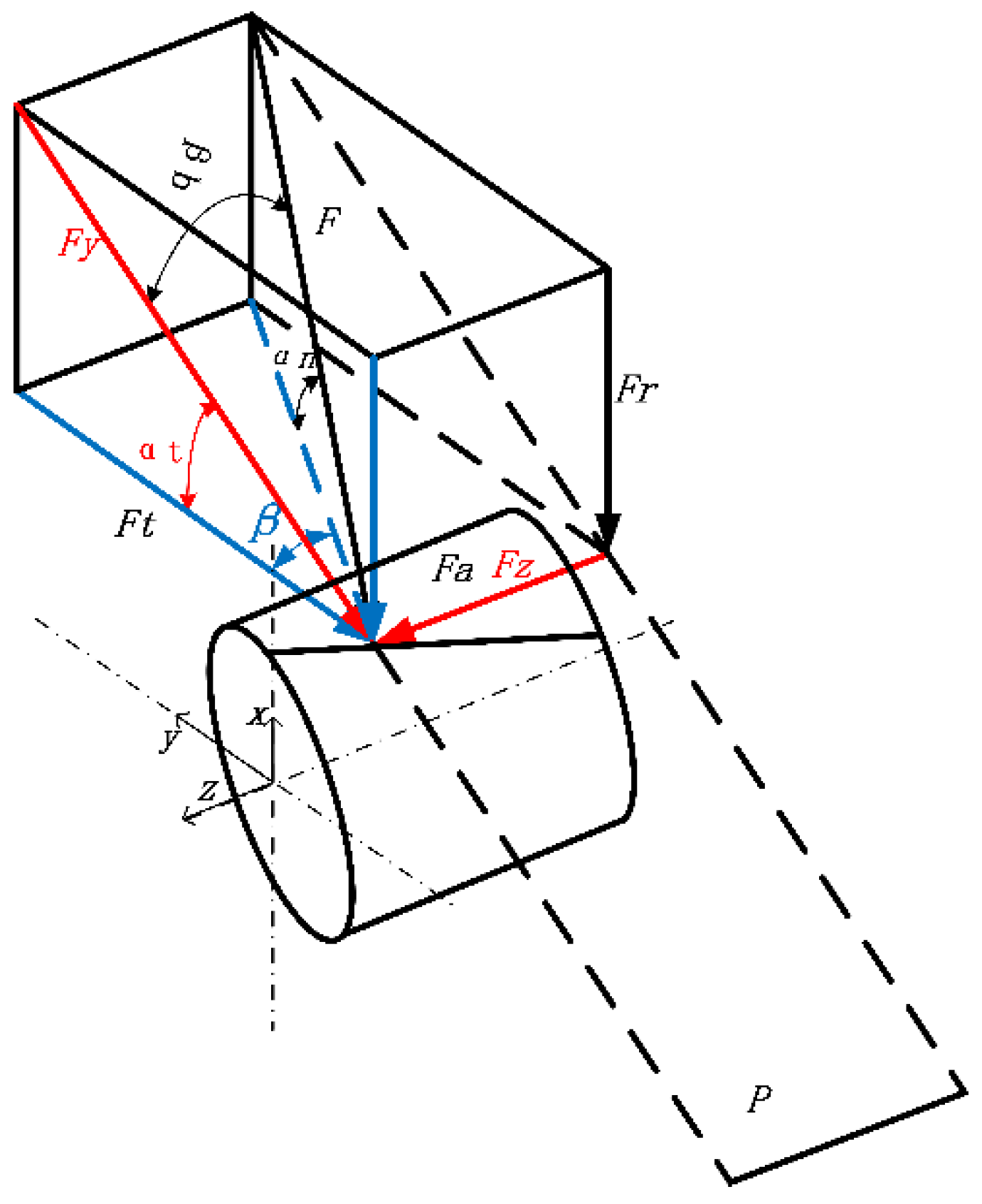
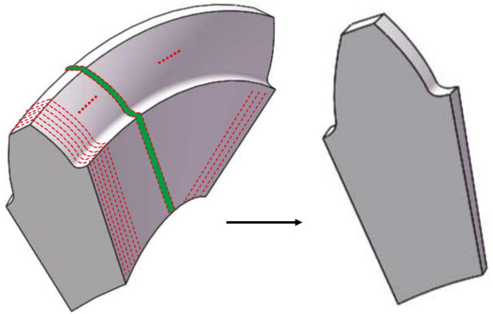
2.1. Computational Formula for Helical Gears with Crack Fault

Figure 1 is the force analysis diagram of helical gear. The axial force in helical gear is an important component of the meshing force, and it can be expressed as:
F a = F cos α n sin β
where α n is the normal pressure angle, β is helical gear helix angle. The method of time-varying meshing stiffness should include the axial components.
The helical gear tooth is sliced along the tooth width, and each slice is regarded as a variable section cantilever beam. According to the theory of material mechanics and elasticity mechanics, the calculation of helical gear stiffness should include not only Hertz contact stiffness, bending stiffness caused by transverse force, shear stiffness and axial compression stiffness but also the axial bending stiffness and axial shear stiffness caused by axial force. In addition, the fillet-foundation deflection should also be included. The calculation method can be given [9] as follows:
d U b = F 2 2 d k b ,   k b = 0 l F 2 2 d U b d z
d U s = F 2 2 d k s ,   k s = 0 l F 2 2 d U s d z
d U r c = F 2 2 d k r c ,   k r c = 0 l F 2 2 d U r c d z
d U a b = F 2 2 d k a b ,   k a b = 0 l F 2 2 d U a b d z
d U a s = F 2 2 d k a s ,   k a s = 0 l F 2 2 d U a s d z
d U h = F 2 2 d k h , k h = E L π 4 ( 1 v 2 ) ,  
where F is the meshing force, d U b , d U s , d U r c , d U a b , d U a s are the bending deformation energy, shear deformation energy, axial compression deformation energy, axial bending deformation energy and axial shear deformation energy of each slice, respectively. k b , k s , k r c , k a b , k a s , are the equivalent bending, shearing, axial compression, axial bending and axial shear stiffness, respectively. k h is the Hertz contact stiffness, G is the shear elasticity modulus, the expression is given [34] as:
G = E 2 ( 1 + v )
where E is the elasticity modulus, v is the passion ratio, L is the length of the contact line length.
The total energy of a slice of a pair of meshing teeth in a helical gear pair is:
d U = F 2 2 d k = F 2 2 ( 1 d k b 1 + 1 d k s 1 + 1 d k r c 1 + 1 d k a b 1 + 1 d k a s 1 + 1 d k h + 1 d k b 2 + 1 d k s 2 + 1 d k r c 2 + 1 d k a b 2 + 1 d k a s 2 )
where dk is the total meshing stiffness of a slice unit, 1, 2 represents the driving gear and driven gear of the first-stage, respectively.
Besides tooth deformation, the fillet-foundation deflection also affects the meshing stiffness, so the gear fillet-foundation stiffness should be also considered [5]. The calculation method and parameter selection of fillet-foundation stiffness have been mentioned in the literature [5], so it is not described here. Therefore, the comprehensive meshing stiffness of a single pair of teeth by integrating Equation (9) is described as:
k = 1 / ( 1 k b 1 + 1 k s 1 + 1 k r c 1 + 1 k a b 1 + 1 k a s 1 + 1 k h + 1 k b 2 + 1 k s 2 + 1 k r c 2 + 1 k a b 2 + 1 k a s 2 + 1 k f 1 + 1 k f 2 )
Figure 2 is the schematic diagram of slicing method. When more than one pairs of teeth are engaged, by adding stiffness in Equation (10), the stiffness of multiple pairs can be written as:
k = i = 1 N 1 / ( 1 k b 1 i + 1 k s 1 i + 1 k r c 1 i + 1 k a b 1 i + 1 k a s 1 i + 1 k h i + 1 k b 2 i + 1 k s 2 i + 1 k r c 2 i + 1 k a b 2 i + 1 k a s 2 i + 1 k f 1 i + 1 k f 2 i )
where the N is the number of gears engaged at the same time, i is the ith pair of gears engaged.
During the working process of helical gear, cracks may occur due to the excitation of external motor, road surface and other parts of the transmission system. With the change of meshing angle, the depth and angle of cracks will change and crack propagation will occur. As the meshing stiffness of helical gears changes, the dynamic response of gear transmission system will change.
When the root crack of helical gear occurs, the bending stiffness and the shear stiffness caused by radial force, and the axial bending stiffness and the axial shear stiffness caused by axial force will change. While the axial compression stiffness caused by radial force remains unchanged, and the Hertz contact stiffness remains unchanged.
According to the relationship between the radius of the root circle and the base circle of the gear pair, the stiffness calculation of crack fault is discussed in two cases; only the process in case of r b 1 < r f 1 is deducted in this paper.
Figure 3 is the schematic diagram of helical gear transverse face with crack fault.
We can see from the Figure 3 that when r b 1 < r f 1 , if the operating point of F is inside the crack affected zone, then the cross-section area is:
A x 2 = ( h a + h x 2 ) L , x 2 d a 2 h x 2 L , x 2 > d a
where h a is the distance from crack termination point to tooth centerline, x 2 is the distance from meshing point to root circle, d a is the distance between the end point of the crack on the tooth and the tooth root circle, h x 2 is the distance from the contact point to tooth centerline, and L is the contact line length. When the meshing stiffness of helical gears is calculated by slice method, the contact line length of each slice is d z . The h a and h x 2 are given as:
h a = r b 1 sin α 2 l c 1 sin γ
h x 2 = r b 1 [ ( α 2 α ) cos α + sin α ] , 0 x 2 d a r b 1 [ ( α 2 α ) cos α + sin α ] , d a x 2 d t
where d t is the distance from apex circle to root circle.
The inertia moment can be given by:
I x 2 = 1 12 ( h a + h x 2 ) 3 L , x 2 d a 1 12 ( 2 h x 2 ) 3 L , x 2 > d a
I y 2 = 1 12 ( h a + h x 2 ) ( d z ) 3 , x 2 d a 1 12 ( 2 h x 2 ) ( d z ) 3 , x 2 > d a
Figure 4 is the schematic diagram of a cracked gear tooth with slice method.
We can see from Figure 4 that when cracks occur in helical gears, the axial compression stiffness is not affected, so the axial compression stiffness is calculated [34] by:
1 d k r c 1 = x Q x F sin 2 α n E A x 2 d x 2
where A x 2 is the cross-sectional area at the coordinates.
However, the bending stiffness and shear stiffness caused by radial force as well as the axial bending stiffness and axial shear stiffness caused by axial force are affected.
These parameters are put into the calculation formula of the stiffness, then we get:
1 d k b 1 = x Q x F cos α n cos β ( x F x 2 ) sin α n y F 2 E I x 2 d x 2 = α g α 2 [ cos α n cos β [ r b 1 ( α 2 + α 1 ) sin α 1 + r b 1 cos α 1 r b 1 ( α α 2 ) sin α r b 1 cos α ] sin α n ( r b 1 sin α 2 l c sin γ ) ] 2 E / 12 ( r b 1 sin α 2 l c 1 sin γ + r b 1 [ ( α 2 α ) cos α + sin α ] ) 3 ( d z ) r b 1 ( α 2 α ) cos α d α + α 1 α g cos α n cos β r b 1 [ ( α 2 + α 1 ) sin α 1 + cos α 1 ( α α 2 ) sin α cos α ] sin α n r b 1 [ ( α 2 + α 1 ) cos α 1 sin α 1 ] ] 2 E / 12 ( 2 r b 1 [ ( α 2 α ) cos α + sin α ] ) 3 ( d z ) r b 1 ( α 2 α ) cos α d α
where α g is the involute expansion angle of the point corresponding to the crack termination point G, and it is also the critical angle of the crack affected zone. Debug the program to make the following equation in the critical condition, then we can get the critical angle α g .
r b 1 ( α 2 + α g ) cos α g + l c 1 sin γ = r b 1 sin α 2 + r b 1 sin α g
Using the same method, the shear stiffness caused by radial force can be obtained as:
1 d k s 1 = x Q x F 1.2 cos 2 α n cos 2 β G A x 2 d x 2 = α 1 α g 1.2 cos 2 α n cos 2 β ( 1 + v ) r b 1 cos α ( α 2 α ) E r b 1 [ ( α 2 α ) cos α + sin α ] ( d z ) d α + α g α 2 2 1.2 cos 2 α n cos 2 β ( 1 + v ) r b 1 cos α ( α 2 α ) E ( r b 1 sin α 2 l c 1 sin γ + r b 1 [ ( α 2 α ) cos α + sin α ] ) ( d z ) d α
The axial bending stiffness caused by axial force is written as:
1 d k a b 1 = x Q x F [ cos α n sin β ( x F x 2 ) ] 2 E I y 2 d x 2 = α 1 α g 6 cos 2 α n sin 2 β r b 1 2 [ ( α 1 + α 2 ) sin α 1 + cos α 1 + α 2 α sin α cos α ] 2 ( α α 2 ) cos α E ( d z ) 3 [ sin α + α 2 α cos α ] d α + α g α 2 12 cos 2 α n sin 2 β r b 1 2 [ ( α 1 + α 2 ) sin α 1 + cos α 1 + α 2 α sin α cos α ] 2 E [ r b 1 [ ( α 2 α ) cos α + sin α ] + r b 1 sin α 2 l c sin γ ] ( d z ) 3 r b 1 ( α α 2 ) cos α d α
The axial shear stiffness caused by axial force is given by:
1 d k a s 1 = x Q x F 2 1.2 cos 2 α n sin 2 β ( 1 + v ) E A x 2 d x 2 = α 1 α g 1.2 ( 1 + v ) cos 2 α n sin 2 β E r b 1 [ ( α 2 α ) cos α + sin α ] ( d z ) r b 1 ( α 2 α ) cos α d α + α g α 2 2 1.2 ( 1 + v ) cos 2 α n sin 2 β E ( r b 1 sin α 2 l c 1 sin γ + r b 1 [ ( α 2 α ) cos α + sin α ] ) ( d z ) r b 1 ( α α 2 ) cos α d α
when the contact force is within the influence zone of the crack, the cross-section area is:
A x 2 = ( h a + h x 2 ) L
and the formula for calculating the moment of inertia is:
I x 2 = 1 12 ( h a + h x 2 ) 3 L
where L is the contact line length. When the meshing stiffness of helical gears is calculated by slice method, the contact line length of each slice is d z .
Substitute the above formula into the stiffness calculation formula of crack fault, then the bending stiffness caused by radial force is given by:
1 d k b 1 = x Q x F cos α n cos β ( x F x 2 ) sin α n y F 2 E I x 2 d x 2 = α 1 α 2 A 1 E / 12 ( r b 1 sin α 2 l c 1 sin γ + r b 1 [ ( α 2 α ) cos α + sin α ] ) 3 ( d z ) r b 1 ( α 2 α ) cos α d α
where
A 1 = [ cos α n cos β [ r b 1 cos ( α 1 + α 2 ) sin α 1 + r b 1 cos α 1 r b 1 ( α α 2 ) sin α r b 1 cos α ] sin α n ( r b 1 sin α 2 l c sin γ ) ] 2
Similarly, the shear stiffness caused by radial force is written as:
1 d k s 1 = x Q x F 1.2 sin 2 α n G A x 2 d x 2 = α 1 α 2 1.2 sin 2 α n ( 1 + v ) r b 1 cos α ( α 2 α ) E ( r b 1 sin α 2 l c 1 sin γ + r b [ ( α 2 α ) cos α + sin α ] ) ( d z ) d α
Likewise, the bending stiffness caused by axial force can be described as:
1 d k a b 1 = x Q x F cos 2 α n sin 2 β ( x F x 2 ) 2 E I y 2 d x 2 = α 1 α 2 C E / 12 [ r b 1 [ ( α 2 α ) cos α + sin α ] + r b 1 sin α 2 l c sin γ ] ( d z ) 3 d α
C = cos 2 α n sin 2 β r b 1 2 [ ( α 1 + α 2 ) sin α 1 + cos α 1 α α 2 sin α cos α ] 2 r b 1 ( α α 2 ) cos α
The shear stiffness caused by axial force is written as:
1 d k a s 1 = x Q x F 2 1.2 cos 2 α n sin 2 β ( 1 + v ) E A x 1 d x 2 = α 1 α 2 2 1.2 ( 1 + v ) cos 2 α n sin 2 β E ( r b 1 sin α 2 l c 1 sin γ + r b 1 [ ( α 2 α ) cos α + sin α ] ) ( d z ) r b 1 ( α 2 α ) cos α d α
Figure 5 is the mesh stiffness of cracked gear pair when the axial force is neglected and considered, respectively. The stiffness reduced 0.7 × 10⁸ N/m after the axial force is considered in the method. It is shown that the stiffness decreased by 25%. This is because the axial bending and the axial shear stiffness reduces when a crack fault happens.

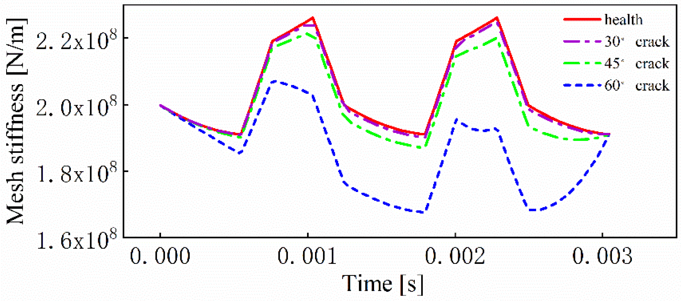
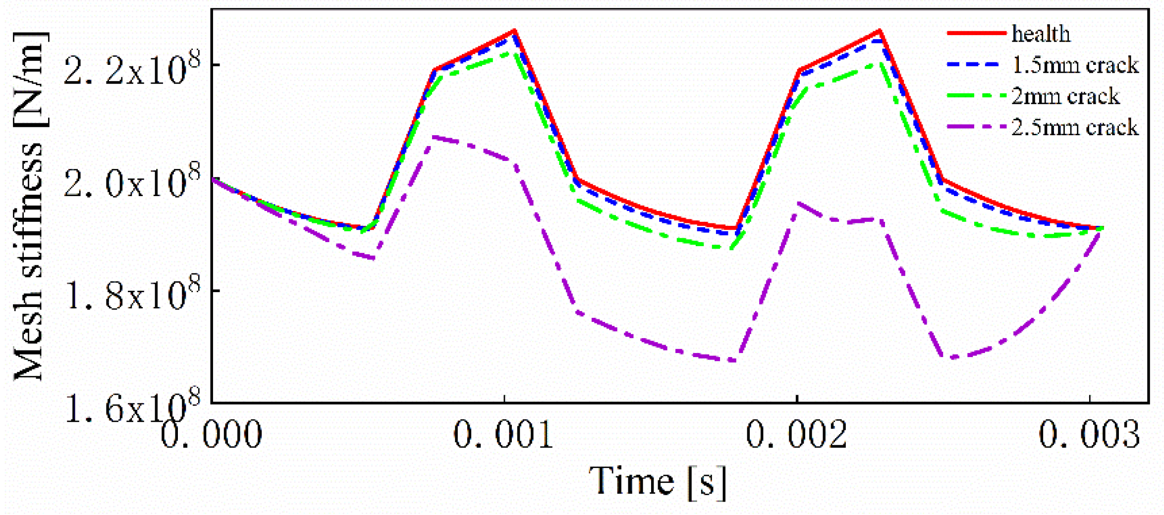
2.2. Influence of Crack Parameters on the Time-Varying Meshing Stiffness

The tooth root crack of helical gear can be determined by the depth of crack on the front l c , the crack angle γ on the front end face and crack length q . The influence of crack parameters on meshing stiffness is studied by analyzing the change of stiffness values of parameters under different values. According to the helical gear pairs listed in Table 1, the influence of parameters on time-varying meshing stiffness is analyzed. The driving gear speed is 3000 r/min. The tooth profile parameters of helical gear pair are shown in Table 1. The module is selected according to the literature [35]. The Young’s modulus and the Poission’s ratio are selected according to the value of steel in the Ansys/workbench.
When the crack length q is 10 mm, the crack depth l c of the transverse face is 2.5 mm, the stiffness is calculated. It is calculated when crack angle is 30 degrees, 45 degrees and 60 degrees, respectively. It can be seen from the Figure 6 that time-varying meshing stiffness reduces when crack fault occurred. With the increase of crack angle, the meshing stiffness of cracked gear decreases more seriously. When the crack angle is 30 degrees, the amplitude decreases by 0.1 × 10⁷ N/m.
When the crack angle γ at the transverse face is 60 degrees, the influence of crack depth parameter l c is studied with the crack length q 10 mm. The results in Figure 7 show that with the increase of crack depth, the amplitude of crack stiffness decreases more obviously. The stiffness decreases by 2.5 × 10⁷ N/m when the crack depth is 2.5 mm. This is because the cross-sectional area and the moment of inertia reduces with the change of crack angle and depth.

3. Establishment of Dynamic Model

y 12 , y 34 is the normal vibration displacement along gears 1 and 2, and gears 3 and 4, respectively, and their expressions are as follows.
y 12 = ( ( x 1 x 23 ) cos α t + ( y 1 y 23 ) sin α t + r 1 θ 1 r 2 θ 2 ) cos β b + ( z 1 z 23 ) sin β b e 12 y 34 = ( ( x 23 x 4 ) cos α t + ( y 23 y 4 ) sin α t + r 3 θ 3 r 4 θ 4 ) cos β b + ( z 23 z 4 ) sin β b e 34
where e 12 is transmission error between gears 1 and 2, e 34 is transmission error between gears 3 and 4. The expression of the two errors is written as:
e 12 = e 0 + e r cos ( w t + ϕ ) e 34 = e 0 + e r cos ( w t + ϕ )
where b 12 is the clearance between gear 1 and 2, b 34 is the clearance between gear 3 and 4. The expressions of the displacement are:
f ( y 12 ) = y 12 b 12 , y 12 b 12 b 12 , b 12 y 12 b 12 y 12 + b 12 , y 12 b 12 f ( y 34 ) = y 34 b 34 , y 34 b 34 b 34 , b 34 y 34 b 34 y 34 + b 34 , y 34 b 34
The normal meshing forces between gears 1 and 2 and between gears 3 and 4 are:
F 12 = k f ( y 12 ) + c f ˙ ( y 12 ) F 34 = k f ( y 34 ) + c f ˙ ( y 34 )
where F y 12 , F z 12 , F y 34 , F z 34 represents the components of contact force of gear 1 and 2 along the transverse direction and axial direction, the components of contact force of gear 3 and 4 along the transverse and axial direction, respectively, and they can be expressed as follows.
F y 12 = F 12 cos β b F z 12 = F 12 sin β b F y 34 = F 34 cos β b F z 34 = F 34 sin β b
The transmission system of pure electric vehicle is typically composed of motor, gear, bearing, elastic shaft and output half shaft of the transmission system. Therefore, a 15 DOF dynamic model of a two-stage helical gear transmission system is established in this paper, as shown in Figure 8a. In Figure 8b, T p is the input torque of the motor, and T g is the load torque, representing the moment of resistance to the wheel.
The model established has fifteen degrees of freedom, including the x , y , z and θ of the driving gear 1, driven gear 4, the x , y , z of the gear 2 and 3 as well as the rotation of gear 2 and gear 3. The dynamic equations are shown as follows.
The dynamics equation of the driving gear on the first level is described as:
m 1 x ¨ 1 + k x 1 x 1 + c x 1 x ˙ 1 = F y 12 cos α t m 1 y ¨ 1 + k x 1 y 1 + c x 1 y ˙ 1 = F y 12 sin α t m 1 z ¨ 1 + k x 1 z 1 + c x 1 z ˙ 1 = F z 12 J 1 θ ¨ 1 = T p r 1 F y 12
The dynamics differential equation of gears on intermediate shaft is given by:
( m 2 + m 3 ) x ¨ 23 + k x 23 x 23 + c x 23 x ˙ 23 = F y 12 cos α t F y 34 cos α t ( m 2 + m 3 ) y ¨ 23 + k x 23 y 23 + c x 23 y ˙ 23 = F y 12 sin α t F y 34 sin α t ( m 2 + m 3 ) z 23 + k x 23 z 23 + c x 23 z 23 = F z 1 F z 2 J 2 θ ¨ 2 = F y 12 r 2 ( c 23 ( θ ˙ 2 θ ˙ 3 ) + k 23 ( θ 2 θ 3 ) ) J 3 θ ¨ 3 = ( c 23 ( θ ˙ 2 θ ˙ 3 ) + k 23 ( θ 2 θ 3 ) ) F y 34 r 3
The dynamics differential equation of gear on output shaft is written as:
m 4 x ¨ 4 + k x 4 x 4 + c x 4 x ˙ 4 = F y 34 cos α t m 4 y ¨ 4 + k y 4 y 4 + c y 4 y ˙ 4 = F y 34 sin α t m 4 z ¨ 4 + k x 4 z 4 + c z 4 z ˙ 4 = F z 34 J 4 θ ¨ 4 = r 4 F y 34 T g
where x , y , z , respectively, represents the displacement in three directions, and the subscripts represent gears 1 to 4. θ is the torsional degree, p , g represents the driving and the driven gear, α t is the end pressure angle of helical gear. The parameters selected of the system are shown in Table 2.

4. Analysis of Dynamic Characteristics of Transmission System

4.1. Experimental Test

Figure 9 is the test of the two-stage transmission system. A two-stage electric drive system test platform is built, as shown in Figure 9a. The system consists of driving motor, two-stage helical gear reducer, half shaft, torque speed sensor, loading motor, controller, accelerometer and so on. The transmission system parameters used are shown in Table 1.
The accelerometer SAE30001 made in Shi’ao Technology is used in this system. The voltage sensitivity is 500 Mv/g. The vibration accelerometer is installed at the bearing of the two-stage drive system near the first driving gear on the gearbox. The sampling frequency of the accelerometer used is 40 kHz. After working for 10 min, with the system working stablely, data is sampled for approximately 2 min.
A 10 N.m torque is applied to the transmission system. The motor input speed is set as 3000 rpm, the same parameters as the simulated. The vibration acceleration data is obtained in the upper computer.

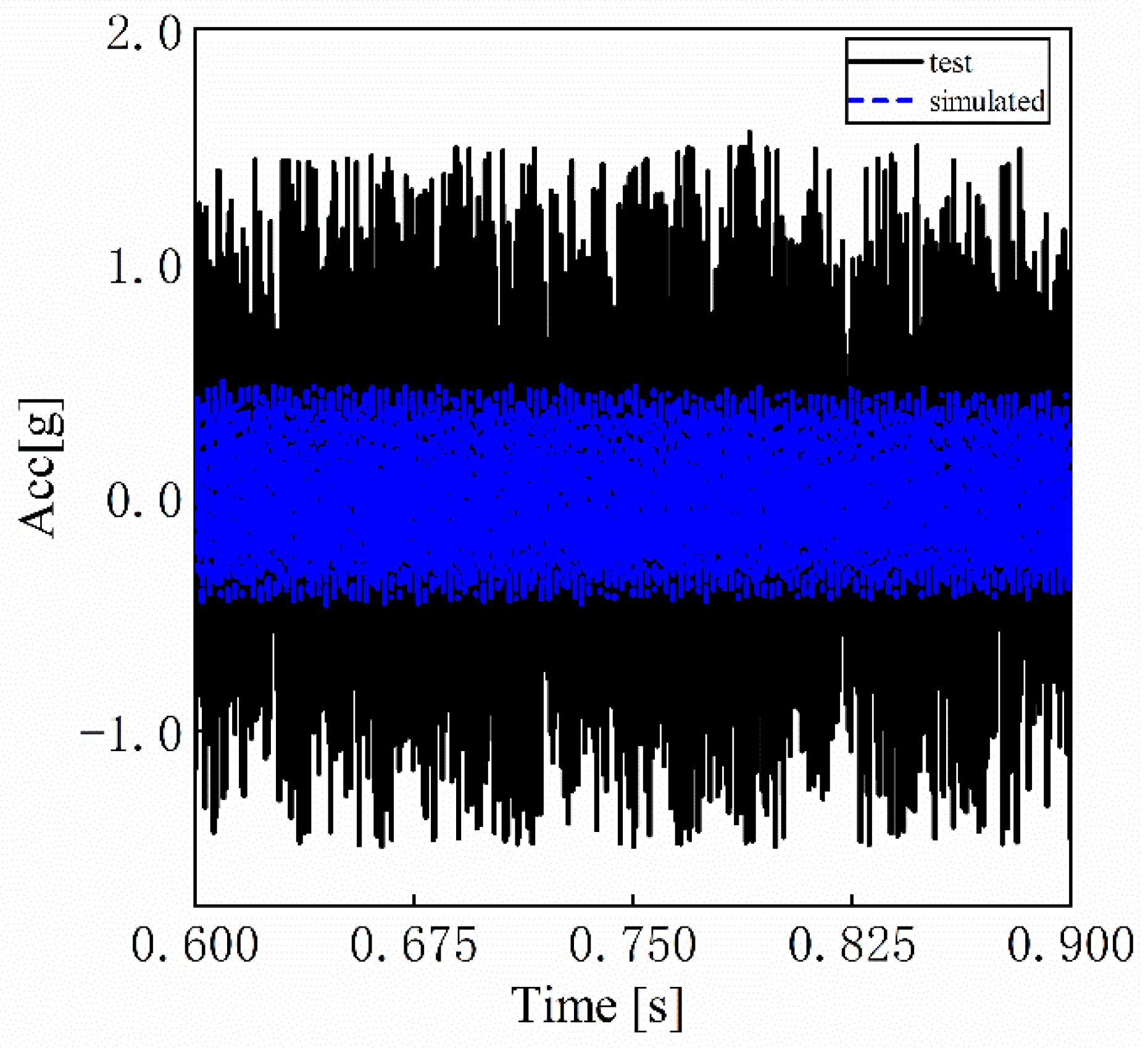
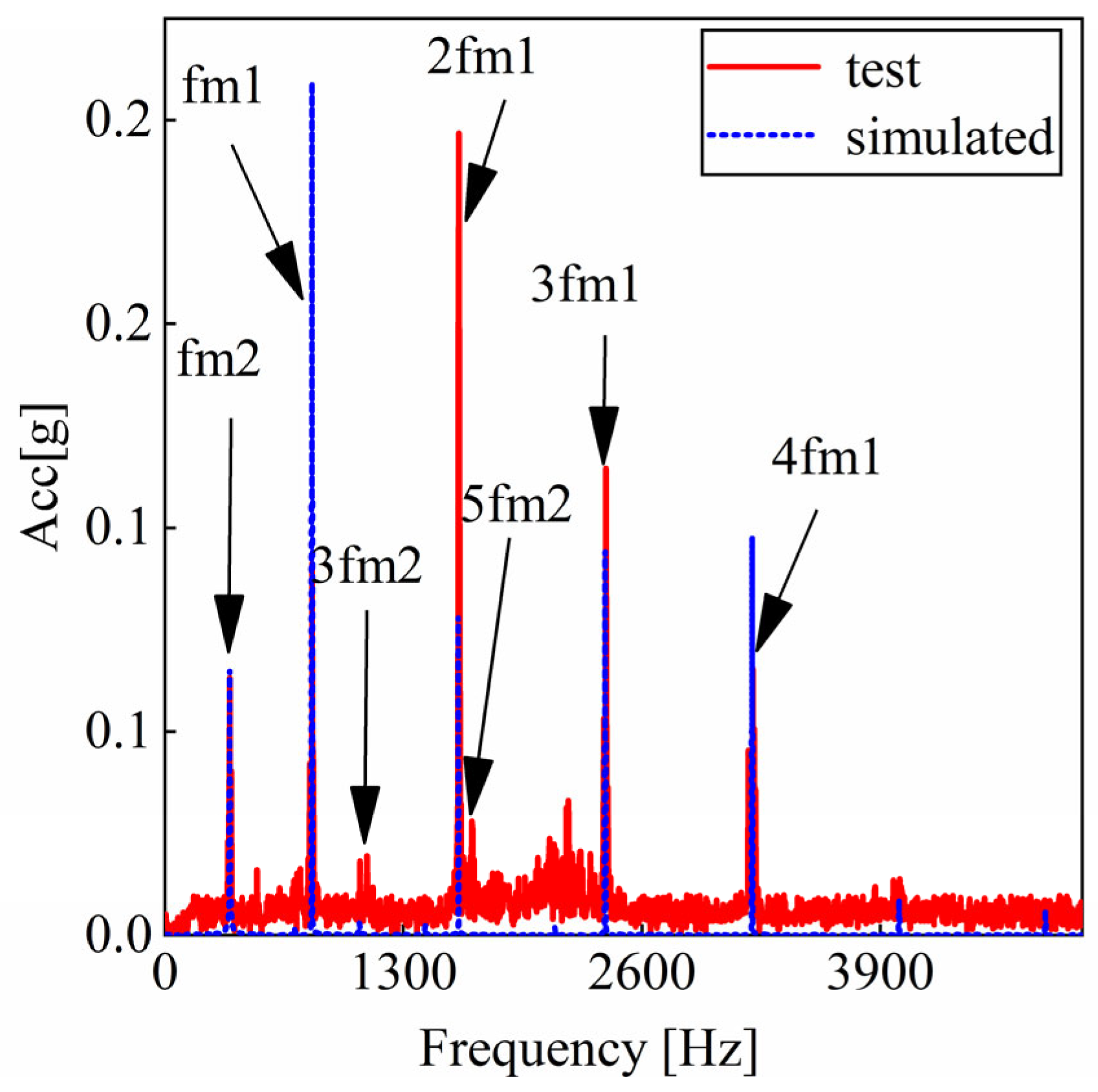
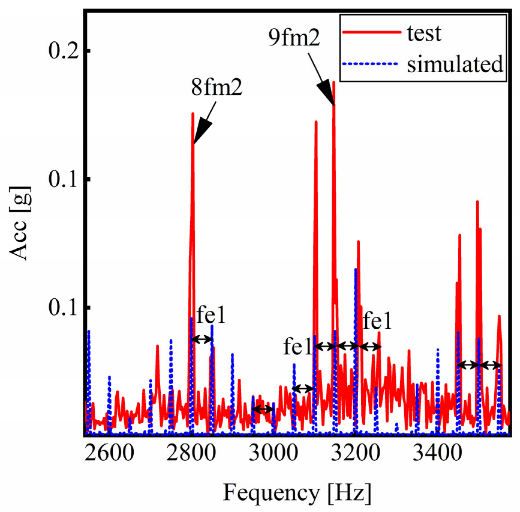
4.2. Analysis of the Simulation and Test Result

The dynamics model of the transmission system established in the above part is solved using Runge-Kutta method. The improved method is used to calculate the stiffness of the gear with crack fault and the gear under normal state. The calculated stiffness is used in the dynamics model.
It is assumed that a crack fault occurs on a tooth of a high-speed driving gear in the transmission system, with the parameters of 10 mm length, 2.5 mm depth, and 30 degrees angle. Figure 10 shows the test and simulated result under normal state in time domain. There appears regular vibration in the test and simulated vibration, and there is no obvious impact in the vibration.
Figure 11 is the test and simulated vibration result under healthy state in the frequency domain. Fourier transform is applied to the experimental and simulated acceleration in time domain. Then, we get the data in frequency. The blue line represents the simulated acceleration vibration, and the red line represents the test data. There are mesh frequency f m 1 of the first gear pairs, mesh frequency f m 2 of the second gear pairs, the harmonic frequencies of the mesh frequency 2 f m 1 , 3 f m 1 , and 4 f m 1 in the frequency domain under normal state. The amplitude at harmonic frequencies is smaller than that of the gear mesh frequency f m 1 and f m 2 . The simulated result is consistent with the test data. This indicates that the dynamic model is correct.

5. Dynamic Characteristics Analysis of Transmission System with Crack Fault

5.1. Influence of the Crack on Vibration Response of Transmission System

Figure 12 shows the test and simulated result of the first gear under fault state. The blue line is the simulated acceleration vibration in time domain, and the black line represents the test acceleration vibration. Choosing 0.3 s as the analytical time, there is a small deviation between the simulated signal and the test data. This is because there is a small deviation of starting time between the simulated data and the test data. There appear regular impacts in the test and the simulated vibration, and the time T is the rotation frequency. This is the time of the input shaft rotating a cycle. In time domain, the result of the simulated is consistent with the test data. The amplitude of vibration is larger than that under normal state.
In order to analyze fault signals more clearly, the difference between vibration acceleration in faulty state and that in normal state in time domain is defined as the residual signal. Figure 13 is the result of residual vibration acceleration under cracked state over time. The depth of the crack is 2.5 mm and the crack angle is 30 degrees. In Figure 13, T is 0.02 s, which is the time for a gear rotating a cycle. It is also the rotation period of the shaft the cracked gear located on. This indicates that the periodic impact vibration is caused by the crack fault. The impact amplitude is approximately 3 g. TC is 0.0030431 s, which is the time required for the crack tooth from engagement to disengagement completely. The t1 represents the time one gear rotating from the tooth after the cracked one. Working to the time t2, the cracked tooth starts to enter mesh. After the time TC, the cracked tooth disengages completely. Then, the tooth after the cracked one enters meshing, starting the next cycle from the time t3. Telling the impact time, we can deduce which gear is faulty in the two-stage helical system.
Figure 14 is the vibration result in frequency domain. Fourier transform is applied to the test and simulated data in time domain data in Figure 12. The red line represents the test acceleration in frequency domain, and the blue represents the simulated result. There appears sidebands around the frequency of the mesh frequency and its harmonics, and the zoomed plot is shown in Figure 15. The sideband frequency is the rotation frequency of the shaft mounting the faulty gear.

5.2. Influence of the Stiffness Considering Axial Force on Vibration Response with Cracked Fault

The vibration acceleration of the driving gear 1 over time in y-direction under the cracked condition is shown in Figure 16. The gear is cracked with the crack depth of 2.5 mm and the crack angle of 30 degrees. Figure 16a is the vibration acceleration over time with axial force neglected. The amplitude of the impact vibration is less than 6 g. Figure 16b is the vibration acceleration over time considering the axial force. From the Figure 16b, we can see that there are obvious periodic impacts. The amplitude of these impacts increases to more than 6 g, larger than that without considering the axial force. The period of the impacts is T. The T equals to the time used by the shaft mounting the faulty gear to rotate a cycle. The impact characteristics caused by faults in time-domain Figure 16b are more obvious compared with those in Figure 16a. The vibration acceleration increases by 8.3% after the axial force is considered into the stiffness of the crack gear pair. This indicates that the characteristics of the crack fault are more obvious after considering the axial force. This is helpful for the diagnosis of crack faults. The increased impact amplitude suggests that the difference between the stiffness in cracked status and the stiffness under normal status is bigger than compared with the method without considering the axial force. This is because bending stiffness and shear stiffness are reduced due to the crack fault without considering the stiffness calculation of axial force, while with the axial force considered, the deformation resulted by the axial force increases, resulting in the reduction of the axial bending stiffness and axial shear stiffness in addition to the reduction of the bending stiffness and shear stiffness.
The acceleration of the gear on the output shaft of the two-stage gears under the healthy and the faulty state is analyzed in Figure 17. Fourier transform is applied to the vibration acceleration of the driven gear 4 in x direction in time domain. The influence of the crack fault is small on the second gear of the output shaft. The acceleration vibration amplitude of the driven gear of the second-stage at the mesh frequency is reduced only approximately 0.08 g. There is nearly no sidebands around the mesh frequency and its harmonics.

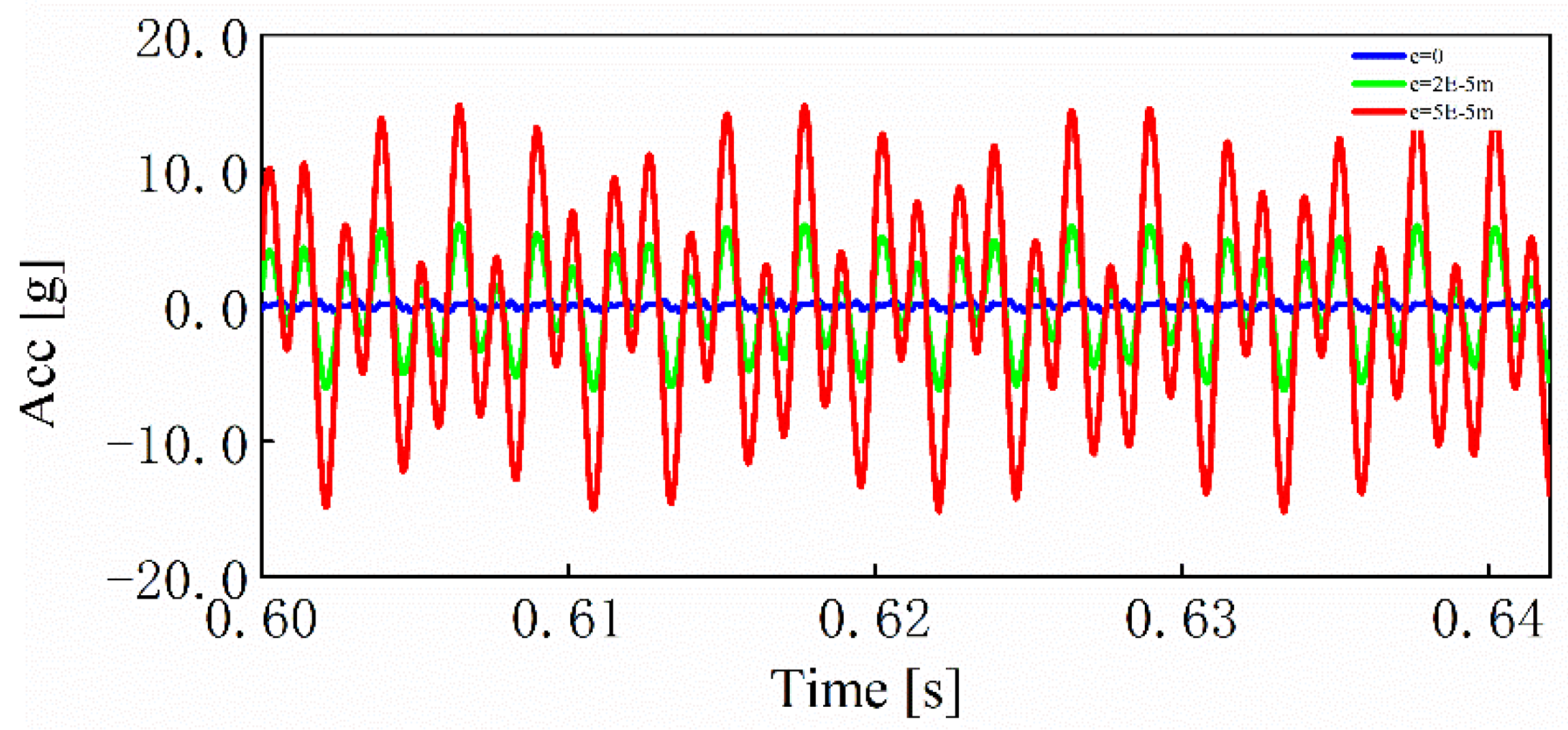
5.3. Influence of Transmission Error on Vibration Response of Transmission System

The vibration acceleration over time with different transmission errors under normal state is shown in Figure 18. The blue, green and red lines represent the vibration acceleration in the y direction in normal state with the 0 error amplitude, 20 um error amplitude and 50 um error amplitude, respectively. It can be seen from Figure 18 that the vibration amplitude with the three errors is approximately 0.5 g, 4 g and 12 g, respectively. With the increase of the transmission error, the vibration acceleration amplitude increases significantly.
Figure 19 is the acceleration signal of gearbox with different transmission errors under faulty condition. Figure 19a shows the vibration acceleration of a cracked gear with the crack depth of 2.5 m, the crack angle of 30 degrees and the crack length of 10 mm when the transmission error amplitude e = 0. The periodic vibration impact caused by the fault can be clearly observed in Figure 19a. The cracked gear starts entering meshing at the moment t2, and at the moment t3, the cracked gear disengages completely. Figure 19b shows the vibration acceleration when e equals to 20 um. The amplitude is approximately 4 g. Periodic impact exists, but it is not obvious as that when e is 0. Figure 19c is the vibration acceleration over time when e is 50 um, and its amplitude is 12 g. The periodic impact is not obvious. It shows that the vibration amplitude increases with the increase of transmission error amplitude e, which is consistent with the conclusion in a normal state. However, the periodic impact characteristics caused by crack faults are submerged heavily, increasing the difficulty of the crack fault diagnosis.

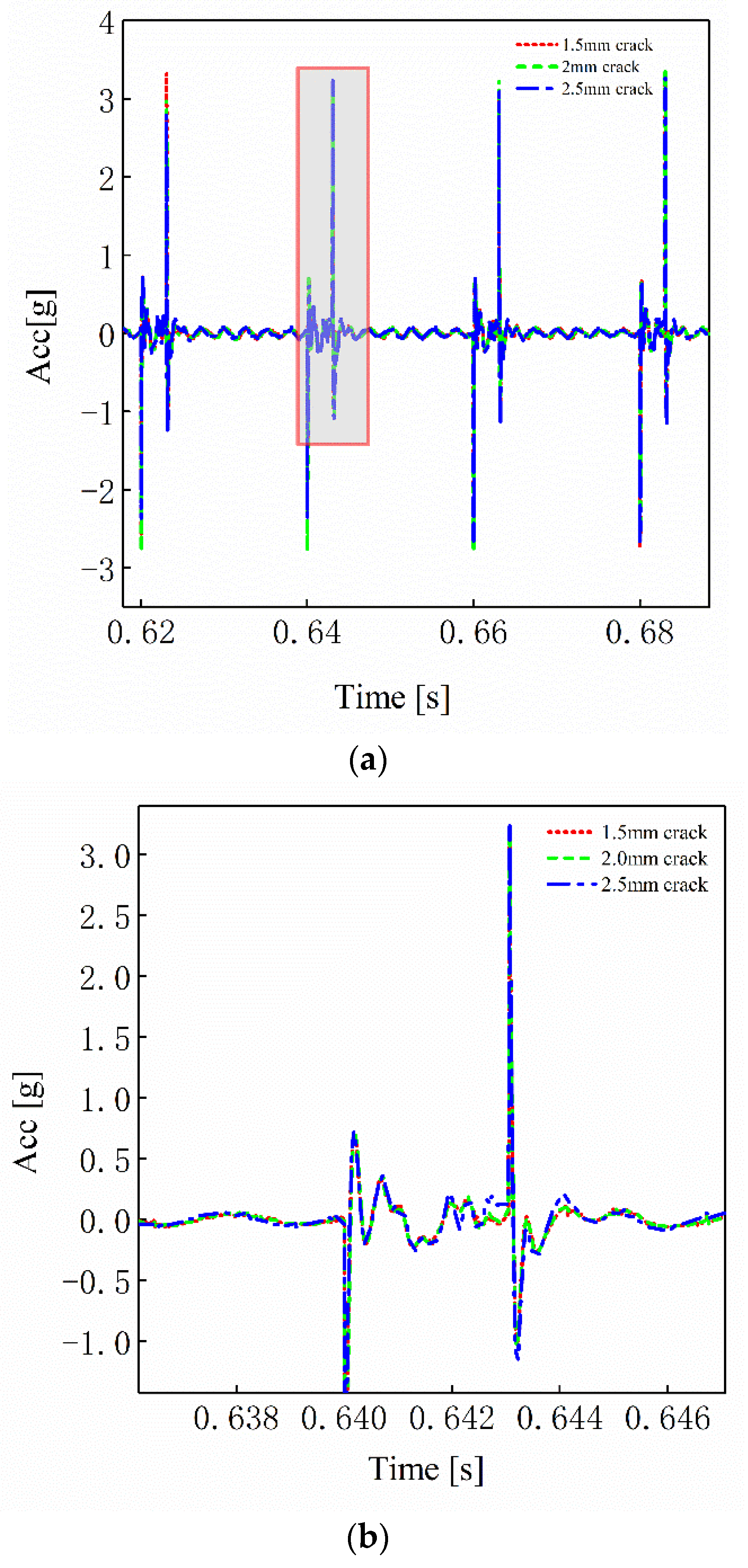
5.4. Influence of Different Crack Parameters on Vibration Response of Transmission System

The vibration characteristics of the transmission system under different crack angles and different crack depths are analyzed. In order to make the crack fault characteristics more obvious, the difference between the vibration acceleration value under faulty state and that under normal state is defined as the residual signal. This signal reduces the interference of the transmission error on the crack fault characteristics. The residual errors of residual errors of gear vibration acceleration at different crack angles over time is shown in Figure 20. The red, green and blue lines show the residual signals of 30 degrees crack, 45 degrees crack and 60 degrees crack with the crack depth 2.5 mm and the tooth length 10 mm (100% gear root width). Figure 20a shows that there exists obvious vibration impact characteristics at the three angles, and the impact amplitude is approximately 3 g. In zoomed plot Figure 20b, it can be seen that the impact amplitude increases as crack angle increases.
Figure 21 is the residual signals of vibration acceleration at different crack depths. Red, green and blue lines represent the residual signal of the 1.5 mm depth crack, 2 mm depth crack and 2.5 mm depth crack over time when the crack length of the root crack is 10 mm, and the crack angle is 60 degrees. Figure 21a shows that the residual impact vibration is obvious when the crack depth is 1.5 mm, 2 mm and 2.5 mm, and the vibration impact amplitude is approximately 3 g. Figure 21b shows that the residual increases with the deepening of the fault depth.
With the increase of crack depth and crack angle, the amplitude of residual signal increases gradually. In order to diagnose the degree of crack fault more sensitively, statistical analysis of crack fault is needed.

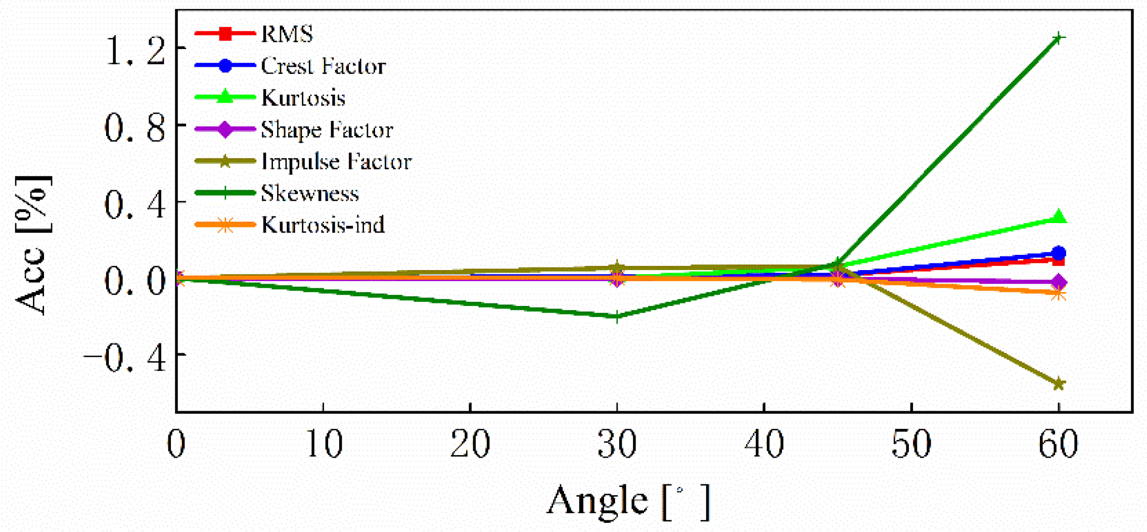
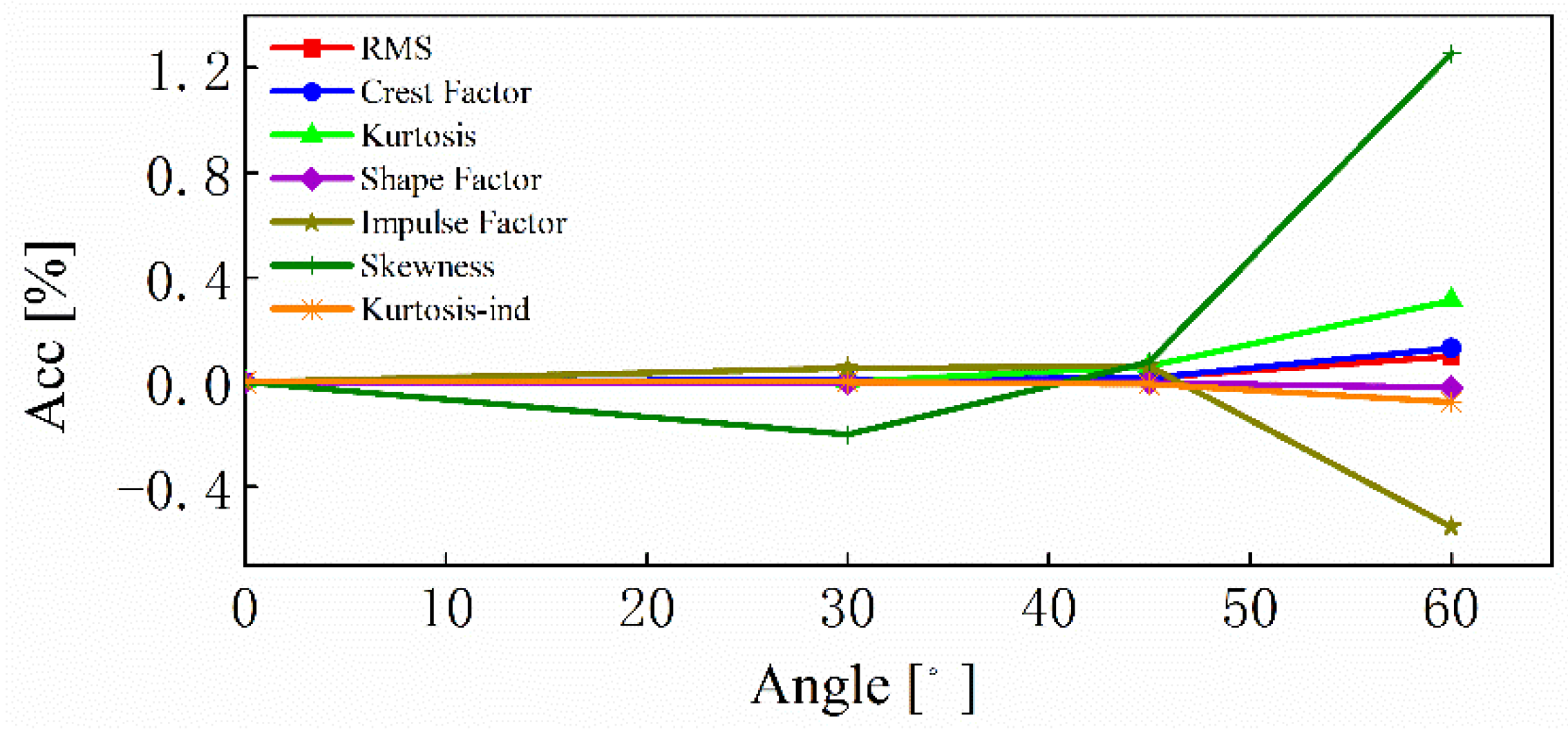
6. Statistical Index Analysis of Time Domain Signal

The degree of crack failure can be evaluated by statistical indexes. The RMS, clearance factor, peak, crest factor, kurtosis, impulse factor, skewness, shape factor and other indicators of time-domain vibration signal are calculated, respectively, to evaluate the level of crack failure. The calculation process of the above statistical indicators has been introduced in the literature [36], so we will not expand in detail here.
In order to reflect the degree of crack failure more sensitively, the method of percentage of statistical indicators is calculated. The percentage can be calculated as follows:
p c = x c x h x h 100 %
where x c is the value of statistical indicators in the faulty state, and x h is the value of statistical indicators in the normal state.
The change of percentages of several statistical indexes when the crack angles increase is shown in Figure 22. As shown in the Figure 22, the skewness first decreases and then increases with the increase of the angle, and the difference is the largest at different angles among the statistical indexes. The impulse factor changes from 0 to −0.6%, which is second only to the skewness. The value of kurtosis changes from 0 to 0.31% as the angle increases from 0 to 60 degrees. The crest factor increases from 0 to 0.13%. The change of RMS is similar to the crest factor, whose value changes from 0 to approximately 0.1%. The shape factor and kurtosis factor change very slowly, almost close to 0, very insensitive to crack.
Figure 23 is the percentage calculation result of these statistical indicators under different crack depths. Similar to the angle curve, the skewness is most sensitive to the change of crack depth. The impulse factor is also sensitive to crack, varying from 0 to approximately −0.55%. The change of kurtosis factor is weak, only from 0 to approximately −0.1%. The least obvious is the lower shape factor, whose change is almost zero.
As can be seen from Figure 22 and Figure 23, the gap between the statistical indicators and the normal condition becomes larger with the deepening of the fault degree. By comparing the percentages of the above statistical indexes at different crack angles and different crack depths, it is concluded that the skewness, impulse factor and kurtosis are more sensitive to the crack, and the sensitivity decreases in turn. It shows that the percentage of skewness can be used as the judging basis for the crack evolution of the helical gear in the transmission system. The conclusion provides a basis for fault diagnosis of crack.

7. Conclusions and Future Work

To analyze the crack influence on two levels of helical gear transmission system, the meshing stiffness is improved. A two-stage dynamic model of the helical gear is established. The influence law of crack parameters on the vibration characteristics is analyzed. The sensitive degree of statistical indicators with a crack is studied in order to better implement the two-stage helical gear fault diagnosis. The following conclusions are drawn.
(1) Considering the axial force with crack fault, the stiffness decreases by 25%. The stiffness reduced more vigorously with the increase of crack depths and angles. The impact amplitude increases by 8.3%. The improved method is more helpful to crack fault diagnosis;
(2) There appears periodic interval under the faulty state in time domain. Sidebands appear around the mesh frequency and the harmonics of the first-stage gear pairs and the second-stage gear pairs, while there is a little influence on the vibration acceleration of the driven gear on the second-stage;
(3) The introduction of transmission error brings interference to the diagnosis of the crack fault. Residual signal can be more useful to diagnose the crack fault of the helical gear;
(4) According to the residual signals in frequency domain and time domain, we can tell by the gear which stage is cracked. While through the time required for the crack tooth from engagement to disengagement completely, we can tell which gear is cracked. we can tell the faulty gear pair of the two-stage helical gear transmission system, while through the impact periodic analysis, we can tell which gear is cracked. This is of great importance to the fault diagnosis in two-stage helical gear transmission system;
(5) The skewness, impulse factor and kurtosis change obviously to the crack fault, and their sensitivity decreases in turn. They can be used for the crack fault diagnosis of the helical gear.
The results proposed can be used for the crack diagnosis of helical gears. However, the dynamic characteristics and data processing method used in the electric transmission system need more efforts to investigate.

Author Contributions

Conceptualization, Y.L.; formal analysis, Y.L., W.W. and K.L.; funding acquisition, S.Y. and W.W.; investigation, Y.L.; methodology, Y.L.; project administration, Y.L.; resources, S.Y. and W.W.; supervision, W.W.; validation, Y.L. and C.L.; visualization, X.S.; writing—original draft, Y.L.; writing—review and editing, W.W., K.L. and X.S. All authors have read and agreed to the published version of the manuscript.

Funding

This work is supported by the National Natural Science Foundation of China (Grant no. U1864210).

Conflicts of Interest

The authors declare no conflict of interest.

Nomenclature

A x 2 the cross-sectional area at the coordinates, m2
A 1 the abbreviation of an expression
b 12 the clearance between gear 1 and 2, m
b 34 the clearance between gear 3 and 4, m
Cthe abbreviation of an expression
c i the torsional damping of drive shaft, N/(m/s)
c x i the bearing damp in the direction of x , N/(m/s)
c y i the bearing damp in direction of y , N/(m/s)
c z i the bearing damp in direction of z , N/(m/s)
d a the distance from the end point of the crack to the tooth root circle, m
d k the total meshing stiffness of wheelset slice unit, N/m
d t the distance from apex circle to root circle
e 12 the transmission error between gears 1 and 2, m
e 34 the transmission error between gears 3 and 4, m
Ethe elasticity modulus, Pa
F the meshing force, N
F 12 the contact force of gear 1 and 2 on the normal surface, N
F 34 the contact force of gear 3 and 4 on the normal surface, N
F a the axial force, N
f e 3 the rotation frequency of the output shaft, Hz
f m 3 the first gear mesh frequency, Hz
f m 2 the second gear mesh frequency, Hz
F y 12 the components of contact force of gear 1 and 2 along the end face, N
F z 12 the components of contact force of gear 1 and 2 in the axial direction, N
F y 34 the components of contact force of gear 3 and 4 along the end face, N
F z 34 the components of contact force of gear 3 and 4 in axial direction, N
gthe acceleration of gravity, 9.8 N·kg−1
Gthe shear elasticity modulus, Pa
ithe number of the pair of gears engaged
k b the equivalent bending stiffness, N/m
k s the shearing stiffness, N/m
k r c the axial compression stiffness, N/m
k a b the axial bending stiffness, N/m
k a s the axial shear stiffness, N/m
k h the Hertz contact stiffness, N/m
k x i the bearing stiffness in the direction of x for the gear i, N/m
k y i the bearing stiffness in the direction of y for the gear i, N/m
k z i the bearing stiffness in the direction of z for the gear i, N/m
Lthe length of the contact line length, m
l c the depth of crack on the front, mm
Nthe number of gears engaged at the same time
p c the percentage of statistical indicators
qthe crack length, mm
R b 1 the radius of the base cycle of the driving gear 1, m
R f 1 the radius of the root cycle of the driving gear 1, m
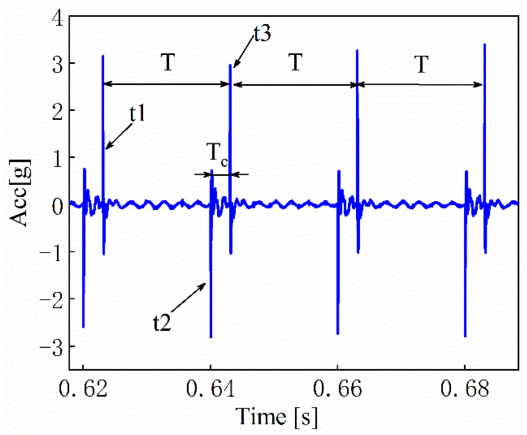
Tthe rotation time of the gear in one cycle, s
tthe time, s
t1the time one gear rotating from the tooth after the crack one, s
t2the time the cracked tooth starts to enter mesh, s
t3the time the tooth after the cracked tooth enters meshing, s
TCthe time required for crack tooth rotating in one cycle, s
T p the input torque of the motor, N.m
T g the load torque, N.m
d U b the bending deformation energy of each slice, J
d U s the shear deformation energy of each slice, J
d U r c the axial compression deformation energy of each slice, J
d U a b the axial bending deformation energy of each slice, J
d U a s the axial shear deformation energy of each slice, J
vthe passion ratio
xthe displacement in the x direction, m
x 2 the distance from meshing point to root circle, m
x c the value of statistical indicators in the fault state
x h the value of statistical indicators in the normal state
ythe displacement in the y direction, m
y 12 the normal vibration displacements along gears 1 and 2, m
y 34 the normal vibration displacements along gears 3 and 4, m
zthe displacement in the z direction, m

Greeks

α n the normal pressure angle, rad
α t the end pressure angle of the helical gear, rad
γ the crack angle on the end face, rad
p the driving gear
g the driven gear
β the helical gear helix angle, rad
θthe torsional vibration, deg.

Abbreviations

RMSthe root-mean-square value

References

  1. Wu, G.; Wu, H.; Li, D. Review of Automotive Transmission Gear Rattle. J. Tongji Univ. 2016, 44, 276–285. [Google Scholar]
  2. Spitas, C.; Spitas, V. Coupled multi-DOF dynamic contact analysis model for the simulation of intermittent gear tooth contacts, impacts and rattling considering backlash and variable torque. Proc. Inst. Mech. Eng. Part C J. Mech. Eng. Sci. 2016, 230, 1022–1047. [Google Scholar] [CrossRef]
  3. Yang, D.C.H.; Lin, J.Y. Hertzian damping, tooth friction and bending elasticity in gear impact dynamics. J. Mech. Transm. Autom. Des. 1987, 109, 189–196. [Google Scholar] [CrossRef]
  4. Tian, X. Dynamic Simulation for System Response of Gearbox Including Localized Gear Faults. Master’s Thesis, Albert University, Edmonton, AB, Canada, 2004. [Google Scholar]
  5. Sainsot, P.; Velex, P. Contribution of gear body to tooth deflections—A new bidimensional analytical formula. Trans. ASME 2004, 126, 748–752. [Google Scholar] [CrossRef]
  6. Wan, Z.; Cao, H.; Zi, Y.; He, W.; He, Z. An improved time-varying mesh stiffness algorithm and dynamic modeling of gear-rotor system with tooth root crack. Eng. Fail. Anal. 2014, 42, 157–177. [Google Scholar] [CrossRef]
  7. Ma, H.; Song, R.; Pang, X.; Wen, B. Time-varying mesh stiffness calculation of cracked spur gears. Eng. Fail. Anal. 2014, 44, 179–194. [Google Scholar] [CrossRef]
  8. Wang, Q.; Zhao, B.; Fu, Y.; Kong, X.; Ma, H. An improved time-varying mesh stiffness model for helical gear pairs considering axial mesh force component. Mech. Syst. Signal Process. 2018, 106, 413–429. [Google Scholar] [CrossRef]
  9. Jiang, H.; Liu, F. Mesh stiffness modelling and dynamic simulation of helical gears with tooth crack propagation. Meccanica 2020, 55, 1215–1236. [Google Scholar] [CrossRef]
  10. Wang, S.; Zhu, R. An improved mesh stiffness calculation model for cracked helical gear pair with spatial crack propagation path. Mech. Syst. Signal Process. 2022, 172, 108989. [Google Scholar] [CrossRef]
  11. Wang, S.; Zhu, R. An improved mesh stiffness model of helical gear pair considering axial mesh force and friction force influenced by surface roughness under EHL condition. Appl. Math. Model. 2022, 102, 453–471. [Google Scholar] [CrossRef]
  12. Wang, S.; Zhu, R.; Xiao, Z. Investigation on crack failure of helical gear system of the gearbox in wind burbine: Mesh stiffness calculation and vibration characteristics recognition. Ocean. Eng. 2022, 250, 110971–110972. [Google Scholar] [CrossRef]
  13. Yan, H.; Wen, L.; Yin, S.; Cao, H.; Chang, L. Research on gear mesh stiffness of helical gear based on combining contact line analysis method. J. Mech. Eng. Sci. 2022, 236, 9354–9366. [Google Scholar] [CrossRef]
  14. Zhang, C.; Dong, H.; Wang, D.; Dong, B. A new effective mesh stiffness calculation method with accurate contact deformation model for spur and helical gear pairs. Mech. Mach. Theory 2022, 171, 104762. [Google Scholar] [CrossRef]
  15. Yang, H.; Shi, W.; Chen, Z.; Guo, N. An improved analytical method for mesh stiffness calculation of helical gear pair considering time-varying backlash. Mech. Syst. Signal Process. 2022, 170, 108882. [Google Scholar] [CrossRef]
  16. Huangfu, Y.; Chen, K.; Ma, H.; Che, L.; Li, Z. Deformation and meshing stiffness analysis of cracked helical gear pairs. Eng. Fail. Anal. 2019, 95, 30–46. [Google Scholar] [CrossRef]
  17. Huangfu, Y.; Chen, K.; Ma, H.; Li, X.; Han, H.; Zhao, Z. Meshing and dynamic characteristics analysis of spalled gear systems: A theoretical and experimental study. Mech. Syst. Signal Process. 2020, 139, 106640–106661. [Google Scholar] [CrossRef]
  18. Lin, T.; Guo, S.; Zhao, Z. Influence of crack faults on time-varying mesh stiffness and vibration response of helical gears. J. Vib. Shock. 2019, 38, 29–36. [Google Scholar]
  19. Tuplin, W.A. Gear-tooth stresses at high speed. Proc. Inst. Mech. Eng. 1950, 163, 162–175. [Google Scholar] [CrossRef]
  20. Kahraman, A.; Singh, R. Interactions between time-varying mesh stiffness and clearance non-linearities in a geared system. J. Sound Vib. 1991, 146, 135–156. [Google Scholar] [CrossRef]
  21. Brethee, K.F.; Zhen, D.; Gu, F.; Ball, A.D. Helical gear wear monitoring: Modelling and experimental validation. Mech. Mach. Theory 2017, 117, 210–229. [Google Scholar] [CrossRef]
  22. Chen, Z.; Zhai, W.; Wang, K. Vibration feature evolution of locomotive with tooth root crack propagation of gear transmission system. Mech. Syst. Signal Process. 2019, 115, 29–44. [Google Scholar] [CrossRef]
  23. Meng, Z.; Shi, G.; Wang, F. Vibration response and fault characteristics analysis of gear based on time-varying mesh stiffness. Mech. Mach. Theory 2020, 148, 103786–103801. [Google Scholar] [CrossRef]
  24. Chen, C. Dynamic Modeling of Two-Stage Planetary Gearbox with Tooth Cracks and Its Dynamic Response Analyses. Master’s Thesis, University of Electronic Science and Technology of China, Chengdu, China, 2017. [Google Scholar]
  25. Wei, C.; Wu, W.; Hou, X.; Yuan, S. Study on Oil Distribution and Oil Content of Oil Bath Lubrication Bearings Based on MPS Method. Tribol. Trans. 2022, 65, 942–951. [Google Scholar] [CrossRef]
  26. Spitas, C.; Spitas, V. Calculation of overloads induced by indexing errors in spur gearboxes using multi-degree-of-freedom dynamical simulation. Proc. Inst. Mech. Eng. Part K J. Multi-Body Dyn. 2006, 220, 273–282. [Google Scholar] [CrossRef]
  27. Shehata, A.; Adnan, M.A.; Mohammed, O.D. Modeling the effect of misalignment and tooth microgeometry on helical gear pair in mesh. Eng. Fail. Anal. 2019, 106, 104190. [Google Scholar] [CrossRef]
  28. Sakaridis, E.; Spitas, V.; Spitas, C. Non-linear modeling of gear drive dynamics incorporating intermittent tooth contact analysis and tooth eigenvibrations. Mech. Mach. Theory 2019, 136, 307–333. [Google Scholar] [CrossRef]
  29. Wang, Q.; Ma, H.; Kong, X.; Zhang, Y. A distributed dynamic mesh model of a helical gear pair with tooth profile errors. J. Cent. South Univ. 2018, 25, 287–303. [Google Scholar] [CrossRef]
  30. Yan, P.; Liu, H.; Gao, P.; Zhang, X.; Zhan, Z.; Zhang, C. Optimization of distributed axial dynamic modification based on the dynamic characteristics of a helical gear pair and a test verification. Mech. Mach. Theory 2021, 163, 104371. [Google Scholar] [CrossRef]
  31. Jiang, H.; Liu, F. Dynamic characteristics of helical gears incorporating the effects of coupled sliding friction. Meccanica 2022, 57, 523–539. [Google Scholar] [CrossRef]
  32. Wei, P.; Deng, S. Time-varying Mesh Stiffness Calculation and Research on Dynamic Characteristic of Two-stage Helical Gear System based on Potential Energy Method. Jixie Chuangdong 2020, 44, 51–57. [Google Scholar]
  33. Liu, J.; Zhao, W.; Liu, W. Frequency and Vibration Characteristics of High-Speed Gear-Rotor-Bearing System with Tooth Root Crack considering Compound Dynamic Backlash. Shock. Vib. 2019, 2019, 1854263. [Google Scholar] [CrossRef] [Green Version]
  34. Sun, G.; Zhao, S. Mechanics of Materials; Shanghai Jiaotong University Press: Shanghai, China, 2006. [Google Scholar]
  35. Zhu, X. Handbook of Gear Design; Chemical Industry Press: Beijng, China, 2004. [Google Scholar]
  36. Sharma, V.; Parey, A. A Review of Gear Fault Diagnosis Using Various Condition Indicators. Procedia Eng. 2016, 144, 253–263. [Google Scholar] [CrossRef]
Figure 1. The force analysis diagram of helical gear.
Machines 10 01052 g001
Figure 2. The schematic diagram of slicing method.
Machines 10 01052 g002
Figure 3. Schematic diagram of helical gear transverse face with crack fault.
Machines 10 01052 g003
Figure 4. The schematic diagram of a cracked gear tooth with slice method.
Machines 10 01052 g004
Figure 5. The mesh stiffness of cracked gear pair when axial force is considered and neglected.
Machines 10 01052 g005
Figure 6. Stiffness values at different crack angles.
Machines 10 01052 g006
Figure 7. Stiffness values at different crack depths.
Machines 10 01052 g007
Figure 8. The two-stage drive system. (a) The physical model. (b) The dynamic model.
Machines 10 01052 g008
Figure 9. The test rig. (a) The helical gear test rig. (b) The gear with crack fault.
Machines 10 01052 g009
Figure 10. Time domain diagram of vibration acceleration of the helical gear in normal state.
Machines 10 01052 g010
Figure 11. Frequency domain diagram of vibration acceleration of the helical gear in normal state.
Machines 10 01052 g011
Figure 12. Time domain diagram of vibration acceleration of the helical gear in faulty state.
Machines 10 01052 g012
Figure 13. Residual vibration acceleration under cracked state over time.
Machines 10 01052 g013
Figure 14. Frequency domain diagram of vibration acceleration of the helical gear in faulty state.
Machines 10 01052 g014
Figure 15. The zoomed plot of Figure 14.
Machines 10 01052 g015
Figure 16. Vibration acceleration under cracked state. (a) Before improved. (b) After improved.
Machines 10 01052 g016
Figure 17. Frequency domain diagram of vibration acceleration of the driven gear in second stage under faulty state.
Machines 10 01052 g017
Figure 18. Time domain diagram of vibration acceleration under different transmission errors.
Machines 10 01052 g018
Figure 19. The acceleration of the gear with crack fault under different transmission error amplitudes. (a) e = 0. (b) e = 20 um. (c) e = 50 um.
Machines 10 01052 g019aMachines 10 01052 g019b
Figure 20. Time-domain diagram of residual error of vibration acceleration at different crack angles. (a) The whole. (b) Zoomed plot.
Machines 10 01052 g020
Figure 21. The residual signal of vibration acceleration with different crack depths. (a) The whole. (b) Zoomed plot.
Machines 10 01052 g021
Figure 22. Change of percentage of statistical index with different crack angles.
Machines 10 01052 g022
Figure 23. Variation of percentage of statistical index with different crack depths.
Machines 10 01052 g023
Table 1. Parameters of gears.
ParametersDriving Gear1Driven Gear1Driving Gear2Driven Gear2
Number of tooth16522371
Normal Module (mm)1.251.251.51.5
Pressure angle (°)20201616
Young’s modulus (Pa)2.11 × 10112.11 × 10112.11 × 10112.11 × 1011
Poission’s ratio0.30.30.30.3
Width of tooth (mm)10101212
Table 2. Stiffness and damping parameters used in the transmission system.
ParametersValueUnit
k x i , i = 1, 23, 48 ∗ 107N/m
k y i , i = 1, 23, 48 ∗ 107N/m
k z i , i = 1, 23, 45 ∗ 107N/m
k i , i = 1, 23, 41.2 ∗ 105N.m/rad
c x i , i = 1, 23, 4500N/(m/s)
c y i , i = 1, 23, 4500N/(m/s)
c z i , i = 1, 23, 4500N/(m/s)
c i , i = 1, 23, 410N.m/(rad/s)
Publisher’s Note: MDPI stays neutral with regard to jurisdictional claims in published maps and institutional affiliations.

