1. Introduction
The fourth industrial revolution demands for intelligence in manufacturing when dynamic data collection and data analytics are needed to support learning the production condition, prognostics, and production health monitoring. Intelligence in these complex processes is generated based on accurate knowledge about the process. Digital metrology of the geometric and dimensional characteristics of the workpiece can be a very useful feature in this paradigm to assist the creation of knowledge about the process and product. Typically, inspection is a human-driven process that is conducted by using cyber-physical systems including Coordinate Metrology Machines (CMM), optical and tactile scanners, and vision systems. Ideally, the human element could be removed entirely, and cyber intelligence could be used to determine whether a manufactured product is up to standards or not. The removal of human subjectivity from the inspection process could lead to better finished parts overall. Therefore, it is important that computers can be taught how to inspect a workpiece, as well as make important decisions about its quality, without the need for human intervention.
To allow learning about the part that is being inspected, multiple cyber tools are used. Whether the inspection is through laser scanning, photogrammetry, structured light scanning, etc., a 3D coordinate representation of the workpiece is generated. Today’s coordinate metrology sensors can collect thousands of 3D data points in a portion of a second from a finished or semi-finished surface in a production line. However, the collected data includes a combination of the real geometric information of the measured object, inspection errors, and the noises resulting from the physical nature of the sensing process. In order to “extract” the desired geometric information of the workpiece from this amalgamation of data, strong data analytics methodologies are needed.
Often the optical metrology data has no underlying information to provide prior knowledge to the data analytics processes, as to the exact orientation of the part, the existence of noise within the scan, or what a defect looks like. It is up to the programmer implementing the system to teach the computer how to do these things. In this paper, a method to remove noise from a laser scan of planar data is introduced.
This task is especially important in workpieces with highly reflective surfaces. As the laser scanning process emits a line of laser light that must be detected by a receiving camera, it is possible for this light to be scattered or for other sources of light to be detected, which causes noise in the resulting scan. This noise will show up in the data set as points that are deviated from the actual surface being scanned. Detecting these points can range in difficulty, as some points may exist far above or below a surface and are then easy to detect. However, other noisy data points may exist much closer to the real data, which can make them near impossible to detect.
2. Literature Review
As Industry 4.0 further becomes the norm for the manufacturing sector, employing intelligent inspection systems is required. Automated inspection has been an important topic for many industries for the past decades, to allow a highly consistent, unaided inspection process while maintaining the desired levels of uncertainties and precision [
1,
2,
3,
4]. Controlling the inspection uncertainty is always a challenging task in automated inspection. The robust design of inspection equipment by modeling the deformations, displacements, vibration, and other sources of the imperfection of the components [
5], or by creating mechanisms with the capabilities for self-calibration [
6] are among the major approaches in reducing the inspection uncertainty by improving the physical inspection components. However, controlling the inspection uncertainties by only focusing on the hardware and the physical equipment is always limited and can become very expensive. Today’s metrology equipment are complex cyber-physical systems, and as it is demonstrated in [
7] the cyber components contribute to controlling the inspection uncertainty no less than the hardware components. It has been discussed in previous research how highly valuable information about the manufacturing process can be extracted from the produced parts directly [
8,
9]. While there is a long history of developments in the inspection and metrology of manufacturing and assemblies, there is a lot of work to be done in reducing the uncertainties in digital metrology [
10]. The new paradigm of digital metrology for inspection of geometric features and dimensional accuracies is described as a cyber-physical system with three major cyber components. These three cyber components are described as Point Measurement Planning (PMP), Substitute Geometry Estimation (SGE), and Deviation Zone Evaluation (DZE) [
11,
12]. In several previous research works the effects of sampling strategy including the number and procedure of data collection on the inspection uncertainty are investigated [
4,
13,
14] and several methodologies for selection of the best set of data points in the inspection process are developed. The main approach in these contributions has been a closed-loop of DZE and PMP. The DZE-PMP loop allows using the gradually learned knowledge about the inspected entity to dynamically decide for revising the data set. Among the developed methodologies, the neighborhood search and the data reduction methodologies for virtual sampling from large datasets have shown very promising results with great potentials for further development and implementation [
4]. In addition, interesting results have been achieved considering the upstream manufacturing process data for PMP to allow modeling the actual manufacturing errors for error compensation or any downstream post-processing operation. The approach is referred to as Computer-Aided Manufacturing (CAM)—based inspection [
15], instead of the typical Computer-Aided Design (CAD)—based inspection.
Estimating the Minimum Deviation Zone (MDZ) based on a set of discrete points for non-primitive geometries is a very challenging task. The problem is even more complex when constrains such as the tolerance envelopes are imposed, for freeform surfaces, and for multi-feature cases. The Total Least Square (TLS) fitting criteria is becoming more popular in coordinate metrology since it has a statistical nature and it is computationally less expensive to solve. Various successful methodologies for TLS and weighted TLS (WTLS) are developed which can be used for error compensation, repair, or post-processing in the manufacturing systems [
2,
8,
10,
16]. Various works have been conducted to develop reliable and quick algorithms for TLS of complex geometries, freeform curves, and sculptured surfaces. As an example, Ref. [
17] presents a strong and fast approach for TLS fitting of Non-Uniform Rational B-Spline (NURBS) surfaces using a method referred to as Dynamic Principal Component Analysis (DPCA).
Dynamic completion of DZE by closed-loop of DZE with PMP and SGE has been the subject of several recent research works. In these contributions, the distribution of geometric deviations gradually evaluated by DZE are used for dynamic refinement of the sampling data points and estimation of fitted substitute geometry [
18,
19,
20,
21]. Intelligence is needed to address the requirement of the three main cyber components of an integrated inspection system, developing the point measurement strategy based on an estimation of the manufacturing errors [
13,
16], or using search-guided approaches to find the best representatives of the manufactured surface [
18] are among the main approaches to assist PMP. The former approach relies on significant knowledge of the manufacturing process and demands for employment of digital twins or the detailed simulation of the manufacturing process. As a result, the solutions can be computationally very expensive and logically neglect the effect of non-systematic manufacturing errors. The latter approach requires a loop of PM-SGE-DZE tasks using learning mechanisms, statistical tools, and artificial intelligence. The efficiency of this approach highly depends on the convergence of the iteration process which in difficult cases it may result in a very time-consuming process.
This paper presents an approach of using a PMP-SGE-DZE iterative loop toward solving a challenging problem in the scanning of highly reflective surfaces. These surfaces can refract and distort optical scanning techniques, leading to noise [
22,
23]. While switching to other methods of examination is possible, these methods can be less efficient, be difficult to automate, or be inappropriate for the geometry being examined [
24,
25]. Noise can lead to inaccurate results in an inspection. While these changes can be seemingly small, they can lead to perfectly acceptable parts being rejected and scrapped. It has been shown in multiple research work how significantly the results of the inspection may vary due to these noises particularly by affecting SGE and DZE evaluations [
20,
21,
26]. As the goal is to have near-perfect inspection without human intervention, it is important that this noise can be accurately removed from the scan data.
There are multiple different noise reduction techniques that have been developed for a variety of situations [
27,
28]. Whether through segmentation of the dataset, non-iterative approaches, or intelligent search algorithms, there are many advantages or disadvantages to the methods. This leads to the need for multiple different algorithms to be developed to suit individual situations. Weyrich et al. [
29] looked at the nearby groupings, or neighborhoods, of points in order to determine whether or not individual points were noise. By using three different criteria, the probability of a point being noise could be determined, and by setting a threshold, the severity of noise reduction could be changed. This is an example of a very localized method, but as it required in-depth analysis of every point within a point cloud, it could take a long time to complete the analysis. Zhou et al. [
30] introduced a non-iterative method that separated the data set into small and large threshold regions and treated them using separate algorithms. Their method was very successful in noise reduction of 3d surfaces and being non-iterative, it ran very quickly. Ning et al. [
31] looked at density analysis for outlier detection in points clouds. By examining the density of points in small areas of high-density point clouds, a reasonable estimation of noise in each area could be conducted. This method was quick and highly effective at removing outliers but could possibly struggle in areas of high-density noise. This is because these areas of noise may have a similar density to the overall point cloud, rendering them similar in the eyes of the algorithm. Wang and Feng [
32] looked specifically at reflective surfaces and utilized the scan orientation of multiple scans to best determine where noise exists in scans of parts with higher complexity. This method had a very high success rate for removing noise, but the requirement of extra scans increases scan time for large parts significantly. Rosman et al. [
33] broke down the data set into smaller, similar, overlapping patches. By examining these patches concurrently, noise could be removed from all patches. This method of denoising was focused more on surface reconstruction than analysis and could possibly smooth real errors within the scan, an undesirable result while searching for errors along the surface. Schall et al. [
34] examined point clusters in a scan. By using a kernel density estimation technique, the likelihood of a point existing on the real surface was determined. Similar to the technique developed by Weyrich et al. [
29], this likelihood was used to classify a point as noise or real data. Like a few of these options, our developed method looks at the point cloud globally. Additionally, the developed method is iterative, but the run time is small due to the relatively low computational complexity.
3. Methodology
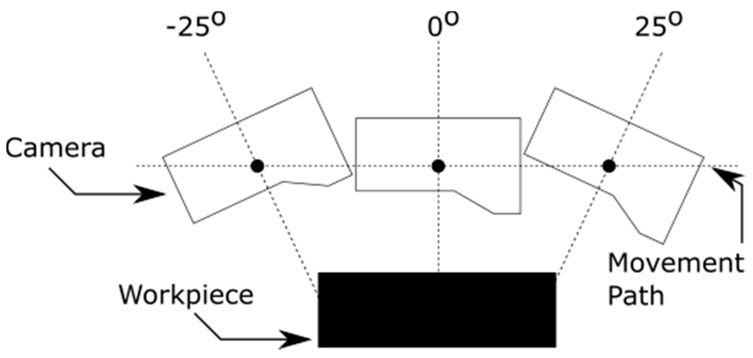
The developed methodology is explained in this section. Although the methodology is implemented for laser scanning using a robotic arm, it can be used for any other coordinate metrology setup. In the current setup, an ABB robotic arm is programmed to iterate through several different motion paths. These paths are designed so that the arm rotates the camera 5 degrees with each pass while maintaining the same vertical distance from the camera center to the workpiece’s surface. As most cameras will provide feedback on the optimal distance of the camera to the workpiece via a bar or color coding, this is used to set the initial distance. In these experiments, an LMI Gocator 2410 with an x-resolution of 0.01 mm is used. The setup is tuned with the camera parallel to the surface in question, so that the 0-degree position will provide the optimal results for the scan, with minimal amounts of noise. The scanning initially begins at the −25 degree points and iterates 5 degrees positively until the −25 degree mark, this process is shown graphically in
Figure 1. The movement path is determined so that the entire workpiece will be captured regardless of the scan angle. All parameters regarding motion speed and path planning, other than the start and end points and the height of the scanner are determined automatically by the robotic control system.
The camera scanning parameters will need to be adjusted for each material scanned, including if the workpiece height changes. These values must be determined for each part used due to variations in material properties and will not be consistent between different workpieces. With an automated algorithm on the robotic arm used in this paper, only the initial position had to be set, then all other positions were calculated automatically based on the programmed scanning pattern. This allowed for all motions to be consistent. Another important aspect of the experiment is the lighting conditions. The scans were all conducted in a controlled setting, with minimal effects of outside lighting present. As this scanning process is an optical one, abrupt changes in lighting conditions can cause a lot of noise to be captured. Another method used to reduce the impact of lighting conditions involved redoing all scans for a workpiece after rotating it 90 degrees. This allowed for the determination of the effects of lighting conditions, for if lighting conditions were an issue, the errors seen would not rotate with the workpiece.
In order to ensure different situations are represented, these tests will need to be rerun for both under and over-exposed conditions. In the underexposed tests, the amount of data captured will be much smaller than in a regular scan. The camera filters out areas of its view that are not a laser and uses the intensity of light of certain wavelengths in order to determine where the laser is. As such, by allowing a smaller amount of light into the viewfinder, more of the laser will not be processed. This leads to datasets without a lot of useful data. This can be beneficial for the reduction of noise, but also leads to situations with a small amount of actual surface information, which could mean the scan misses imperfections on the surface. In the overexposed condition, the opposite occurs, and more light is allowed into the viewfinder. This can lead to noisier point clouds as lower intensity areas of the laser that would typically be filtered out by the software would now be processed as the real surface, while not necessarily being on the real surface.
Once the scans were completed, the background data was removed. This consisted of the plate that the workpiece was laying on. This surface was matte black, and so the data captured for the surface was very consistent with very little noise. A large distance was also maintained between the inspected workpiece surface and the support surface. These factors allowed for the background data to be removed by simply fitting a plane to the data not associated with the actual workpiece surface, then removing it. The collected points (Ps), which will be the input data set, were then exported to the XYZ filetype, which consists of rows of X, Y, and Z coordinates.
Once data collection has been completed, the datasets are imported to the developed software environment to be analyzed. To begin, a plane is fit to the dataset using Total Least Squares (TLS) fitting using the Principal Component Analysis (PCA) method. This is a commonly used algorithm for planar fitting and returns a normal vector and point that defines the fit plane [
35]. The distance between each point of the dataset and the fit plane is then calculated using the point-plane distance calculation shown in Equation (1).
where
A,
B, and
C are components of the fit plane’s normal vector,
x,
y, and
z are the coordinates of a point, and
D is equal to the following.
where
x0,
y0, and
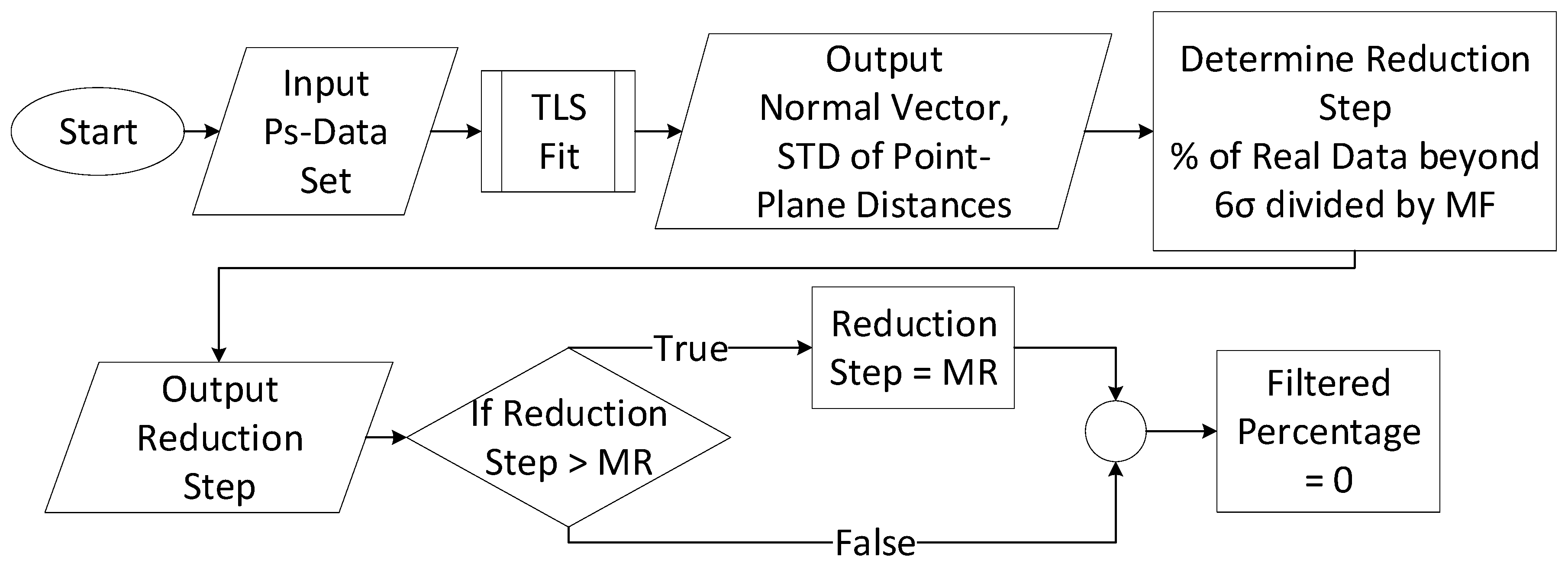
z0 are the coordinates of a point on the plane. With the point-plane distances calculated, a statistical analysis is conducted to determine how many points are beyond the 6σ range. Points beyond this range will be far from the planar surface, so there is a high likelihood that they are noise. The percentage of data in this range is calculated against the entire data set, and this value is divided by a Minimization Factor (MF). This value can control the amount of data being removed at each step. Another check made to ensure too much data is not removed was ensuring that the reduction step did not exceed a Maximum Reduction (MR) step, which is a percentage of the overall data set. The filtered percentage, which tracks how much data is going to be removed, is then set to 0 to initialize the data removal loop. This process is seen in
Figure 2.
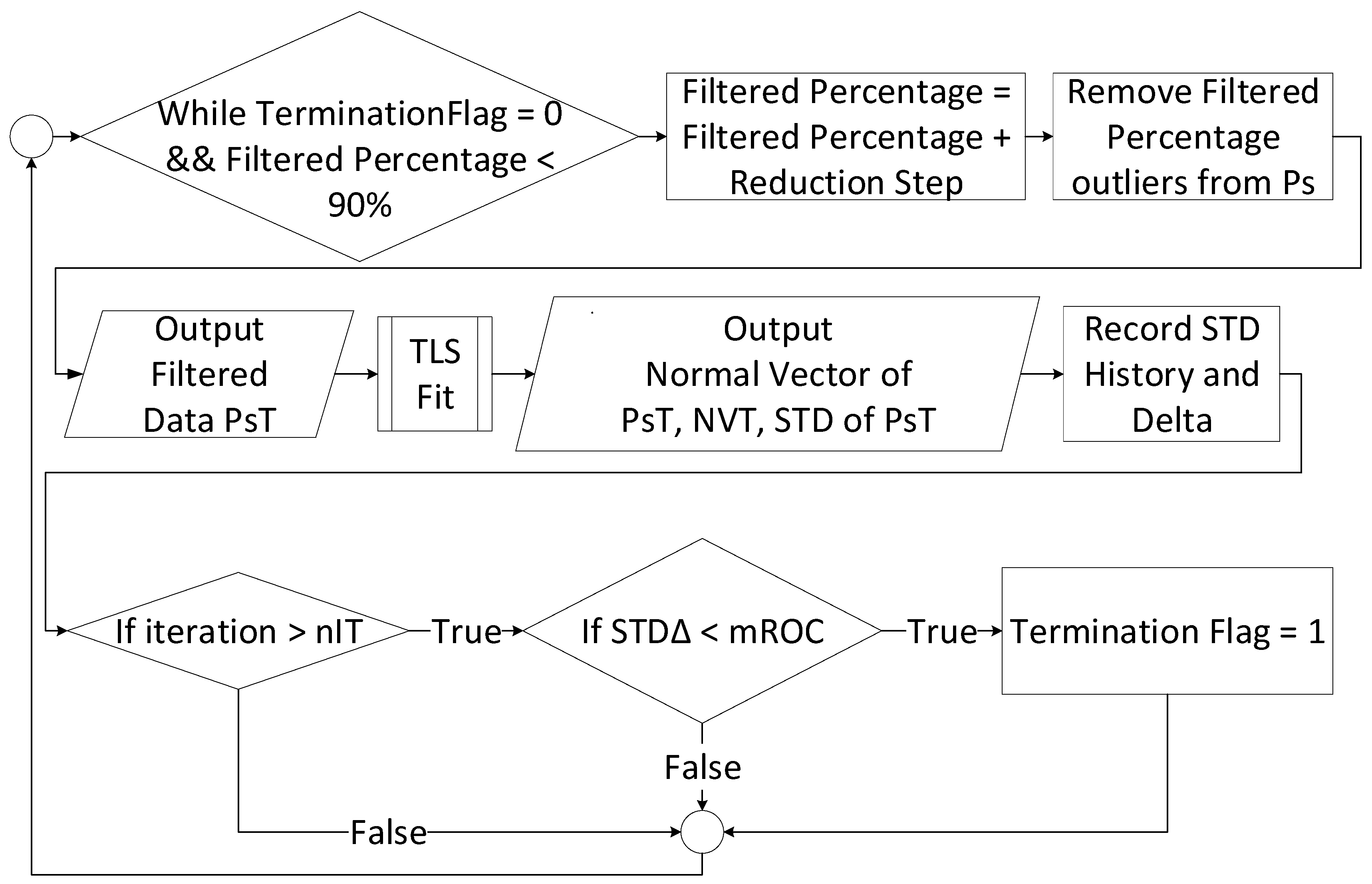
Once the reduction step has been determined, the filtering process begins. In each iteration, the amount of data removed (filtered percentage) increases by the reduction step. This amount of data is removed from the points furthest away from the fit plane. This new data set (PsT), is then fit again with a plane, using TLS. The change in the standard deviation of the point-plane distances is recorded, as well as the rate of change of the same value, these are the standard deviation (STD) history and delta graphs. This process repeats for a set number of iterations (nIT), with each iteration removing more data, as defined by the reduction step. Once the number of iterations has become larger than nIT, a check occurs to determine whether the algorithm can stop with data reduction. This check involves examining the STD delta graph, as it shows the rate of change for the STD. Once the STD delta graph has reached a steady state, determined by the rate of change being less than a minimum rate of change (mROC), the algorithm is stopped. This indicates that the points being removed from the point cloud are likely no longer having a large effect on the STD of the entire point cloud, and thus are unlikely to be outliers. Once this is true, the STD of the point-plane distances of the data set has stabilized. This data reduction algorithm is laid out in
Figure 3.
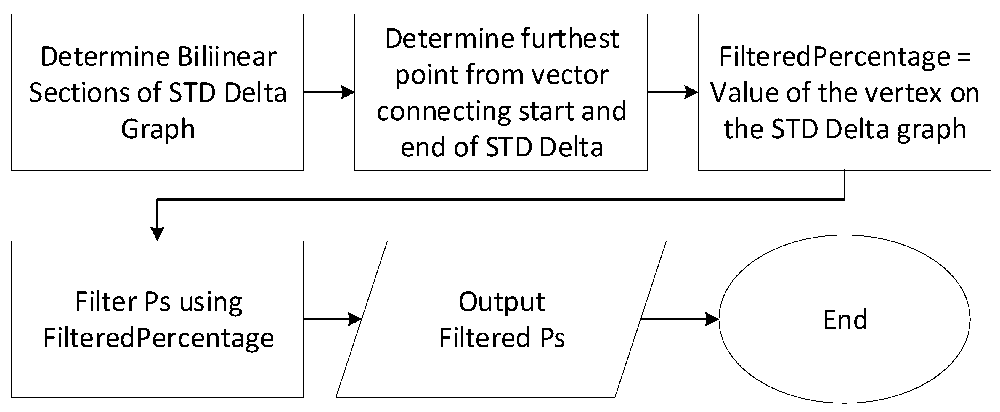
After the data reduction loop has been completed, the amount of data to be removed for the final data set is calculated. This method takes advantage of the general shape of the STD delta graph. An example is shown in
Figure 4.
In the STD delta graph, there is a steep linear section as the STD of the data set decreases, and another linear section with a very flat slope after most outliers have been removed where the STD of the data set is not changing by a significant amount. Once this steady state has been reached, the optimal number of points to be filtered must be determined. In order to accomplish this, the shape of the ideal result is exploited. As the point where the two linear sections meet is the point where the large change in the STD value occurs, the graph is treated as though it is a triangle. The two end points of the STD delta graph are connected to form a line, and the Euclidean distance of each point of the STD delta graph to the line is determined. The furthest point from this line, which would be the vertex opposite the side in the triangle, is selected. The chosen point is the filtered percentage at which the noise removal stopped removing extreme outliers. As the STD delta value begins to remain constant, the points being removed lie closer and closer to the plane. If the filtered percentage is chosen beyond this leveling-off point, actual surface data will likely be removed. The distance is calculated by treating each filtered percentage amount as a point and calculating the Euclidean distance between the intersection point and each filtered percentage amount. The value with the shortest distance is then chosen. The full dataset is then filtered using the specified percentage of removed points, and finally, the filtered data set is returned. This process is fully outlined in
Figure 5.
4. Implementation and Results
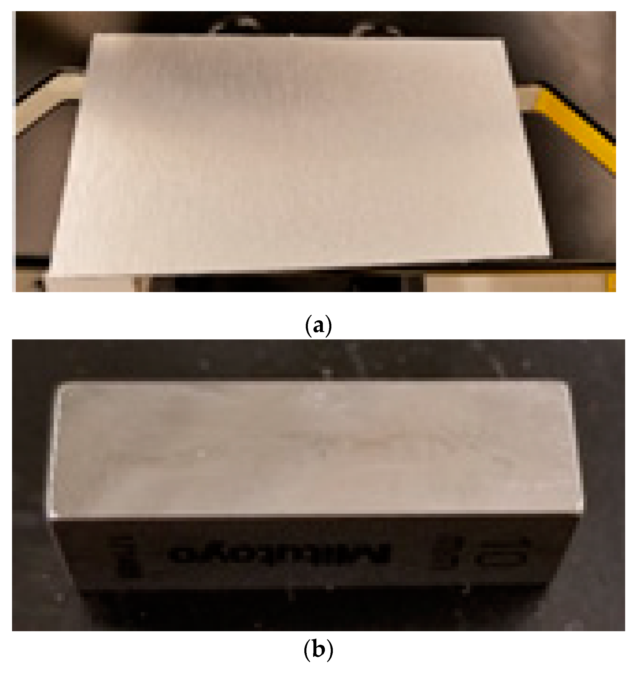
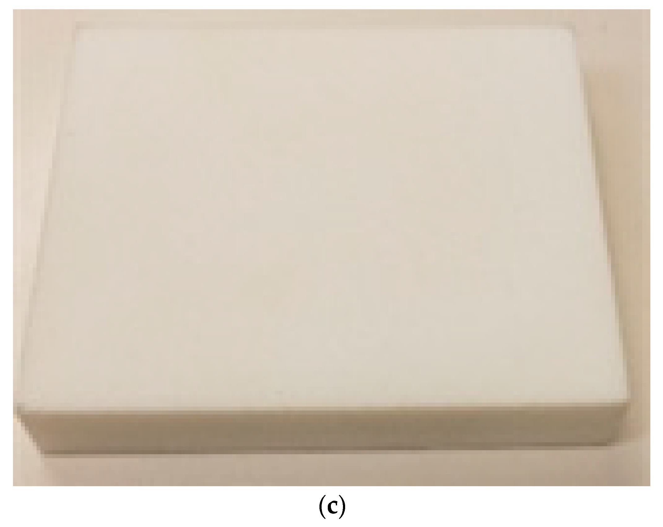
Based on the developed methodology, software was developed to verify its ability to remove noise. Multiple workpieces were analyzed in this study to get a sample of different reflectivity. The variables defined in the methodology were set as follows; minimization factor was 10, maximum reduction step was 0.3, the number of iterations was 10, and the minimum rate of change of 0.005%. These variables were determined through experimentation for the samples chosen. Three samples were used:
- -
a piece of brushed aluminum with flatness of 0.12 mm (
Figure 6a),
- -
a steel gauge block, workshop grade, with flatness of 0.5 µm (
Figure 6b), and
- -
a selective lased sintering (SLS) manufactured part with flatness of 0.08 mm (
Figure 6c).
Figure 6.
Images of three test samples: (a) gauge block; (b) brushed aluminum; (c) SLS printed part.
Figure 6.
Images of three test samples: (a) gauge block; (b) brushed aluminum; (c) SLS printed part.
All objects were selected to have minimal form error to reduce the effects these errors may have on noise generation. These three samples provided unique challenges for scanning. The flatness of the parts is according to the manufacturers’ specifications and verified by a tactile inspection coordinate metrology probe, where applicable. The gauge block had a reflective surface, yet also had a thin film of oil on its surface which reduced the amount of reflection. The SLS part, which is comprised of small, melted granules of plastic, absorbed a lot of the laser light due to its color and had granules on the surfaces which scattered light depending on how they were hit. Finally, the brushed aluminum surface structure had differently oriented grains that reflected light in different manners based on how the light was interacting with them. This was different from the SLS part as the aluminum contained long sections of reflectivity, so it was possible for bands of noise to appear on the part. All these possible sources of error can contribute to the uncertainty of measured values. When determining uncertainty, one of the areas that must be considered is the manufacturer specifications for the device being used to measure the object [
36]. When in a non-standard situation, these specifications may not be accurate. Processing of the data through the use of knowledge of the measurement and conditions can help to reduce the uncertainty of the measurement [
37]. This method may be a useful tool in the reduction of uncertainty of optical scanning of non-ideal material. The results of a few of these tests will be discussed in detail, then the results for the entire test will be shown.
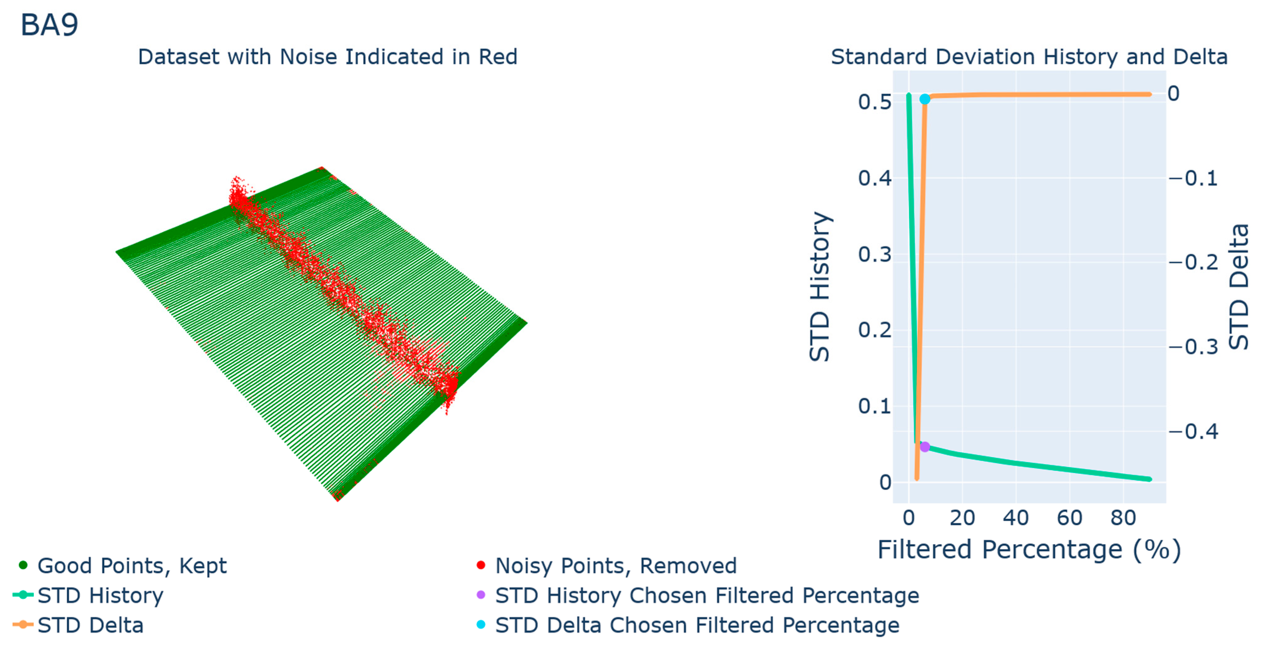
The first sample to be examined is the brushed aluminum at an angle of +15°. There is a band of noise along the center of the piece, highlighted in red in
Figure 7. This is an example of the best-case scenario for the algorithm. The STD delta graph is of the optimal shape, so there is a clear point where the effect of point removal becomes minimal. The deviation zone estimated by the data was reduced by 90.8% through this method with 6% of the point cloud filtered. The STD of deviations was 0.515 mm which was reduced by only 6% filtration to 0.047 mm. The total deviation zone was estimated as 0.113 mm which is fairly close to the known flatness of the part.
The next sample is the gauge block at +10° shown in
Figure 8. The noise in this scan is more distributed throughout the entire surface of the part, both above and below. Again, this situation is ideal. The STD delta graph follows with the shape that is sought after, and a large majority of the noise is filtered from the scan. For this sample, the flatness was reduced by 97.4%. The STD of deviations was 0.512 mm which was reduced by filtration to 0.013 mm. The total deviation zone was estimated as 0.024 mm. Obviously, the gauge block is more precise than the level of accuracy in a laser scanner and the uncertainties in the mechanical and optical features of the measurement device do not allow accurate measurement of a highly precise gauge block. However, the results show that the algorithm was successful in filtering the dominating outlier noises from the data.
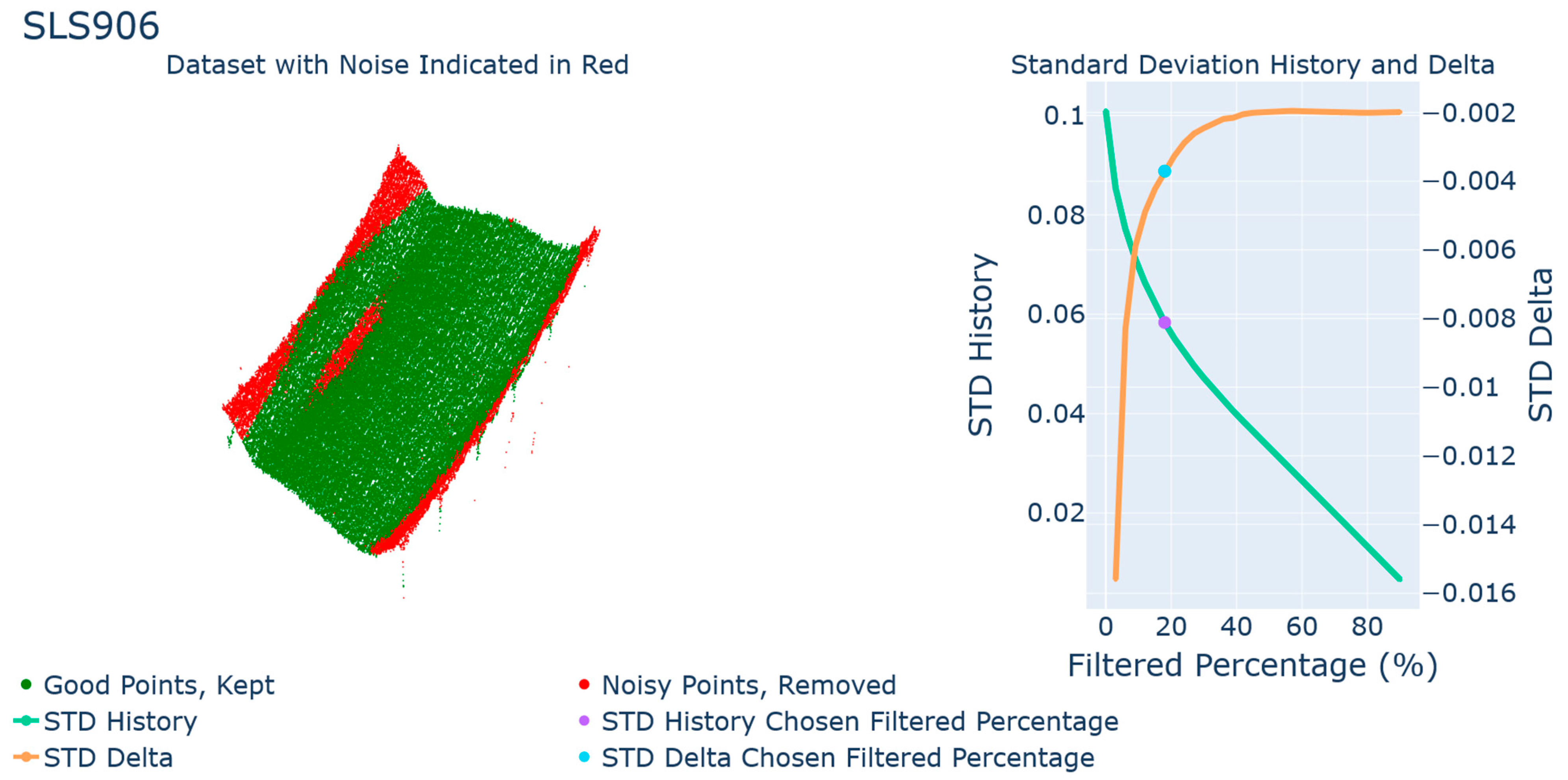
The next sample is the SLS piece, after a 90° rotation, at a scan angle of 0° (
Figure 9). The scan for this part looks cupped due to the capture of the edges of the surface. There is noise shown under the scan. However, the density of the noise is very low. For this scan, there is no initial quick drop in the standard deviation of point-plane distances, which is a less than ideal result. This is due to the relatively small amount of noise having a small effect on the flatness measured when compared to the rest of the data set. There was a reduction of only 38.2% for this sample. The STD of deviation was 0.101 mm which was reduced by filtration to 0.062 mm. The total deviation zone was estimated as 0.153 mm.
After reviewing fairly straightforward cases, a few rare problematic cases are presented in the following. As can be seen, these problematic cases require overly aggressive filtrations with some results that may cause misleading. The next sample is the brushed aluminum piece, with overexposed lighting conditions, after being rotated 90°, at a scan angle of +25° (
Figure 10). This scan had very little noise, however, the removal of the background data was not entirely completed to determine the effect of additional planar data on the algorithm. This resulted in a “stepped” planar surface with two separate heights. In a situation like this, the fit plane would be angled to capture both high-density planar areas. As the surface of the workpiece dominated the scan, a portion of it survived the filtering process, however, a large number of correct scan points was removed due to the initial plane fitting. The STD delta graph shows the wildly varying changes in the data set as points were filtered. Once the secondary background plane was eliminated from the data set, there was no further reduction in the flatness measurement, as the rest of the scan was already ideal. The STD of deviation was 4.51 mm which was reduced by filtration to 0.057 mm. The total deviation zone was estimated as 0.108 mm. While this behavior may seem desirable, it is possible that it could lead to misleading results for an operator or other decision-making process. Fortunately, it is easy to tell from the STD delta graph that something went wrong. This could be used as a diagnostic to ensure scans are occurring correctly.
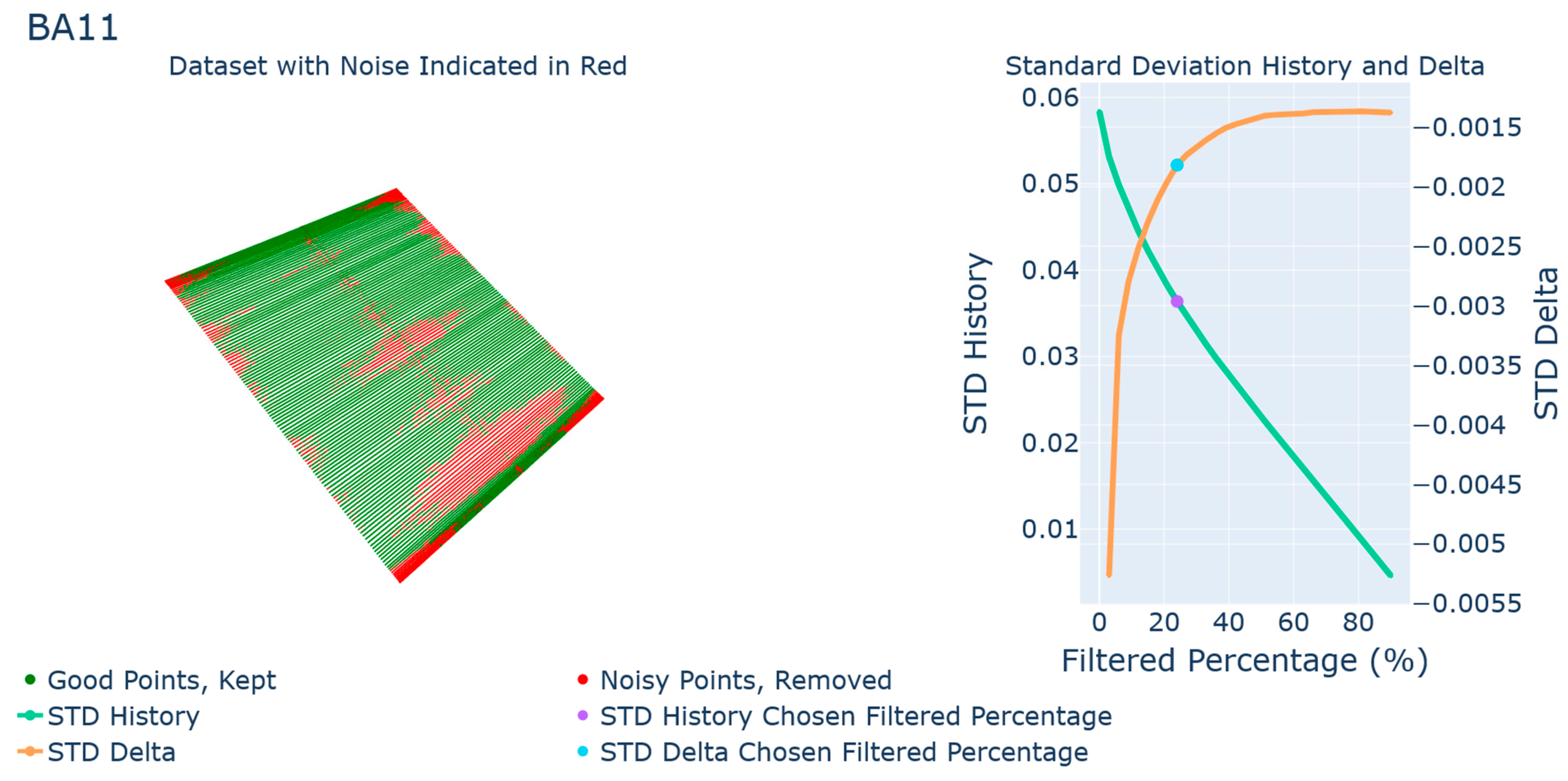
The next example of the problematic cases is brushed aluminum at +25° (
Figure 11). At first glance, the STD delta graph looks to have two bilinear sections, but with a large region of slowing change. The other issue is that the change is quite small to begin with, by only thousandths of a millimeter as indicated by the STD delta scale. This is because the scan had very little noise. As this process is a statistical analysis of the point-plane distances for a data set, if that data set is already very well formed, with only a couple of noisy points standing out from the main data set, the algorithm will overcompensate and begin to remove useful data from the set. This can be seen in the top left picture of
Figure 11, where pieces of the plane have been removed without there being any noise in those areas. Like the previous issue, this can be detected by examining the change in STD over time. If there is a very small change, or if the STD history graph is nearly linear, it is likely that the data set is already very clean. The STD of deviation was 0.058 mm which was reduced by filtration to 0.039 mm. The total deviation zone was estimated as 0.104 mm.
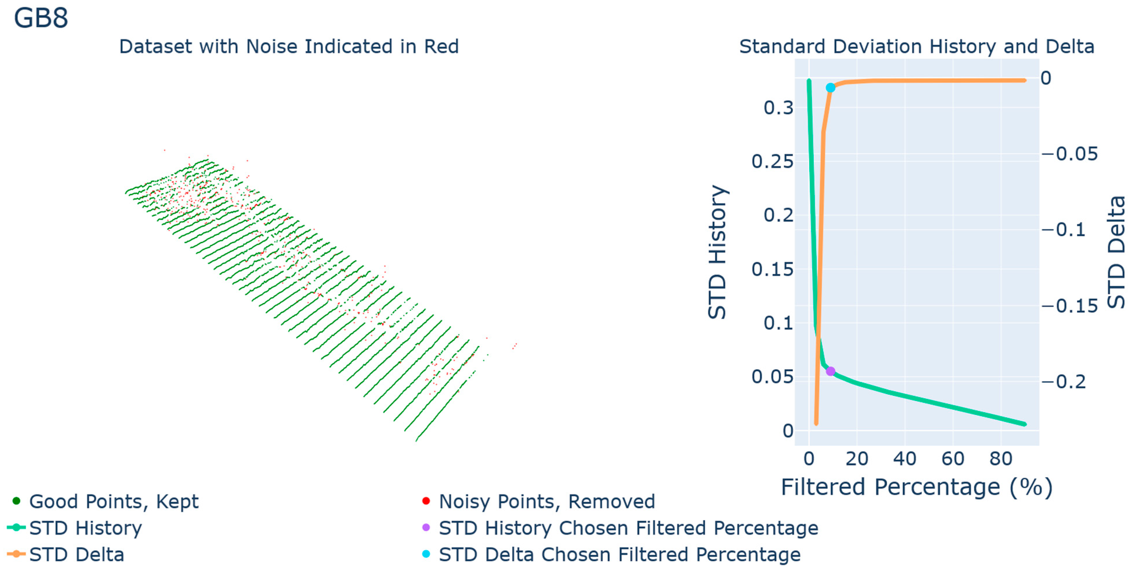
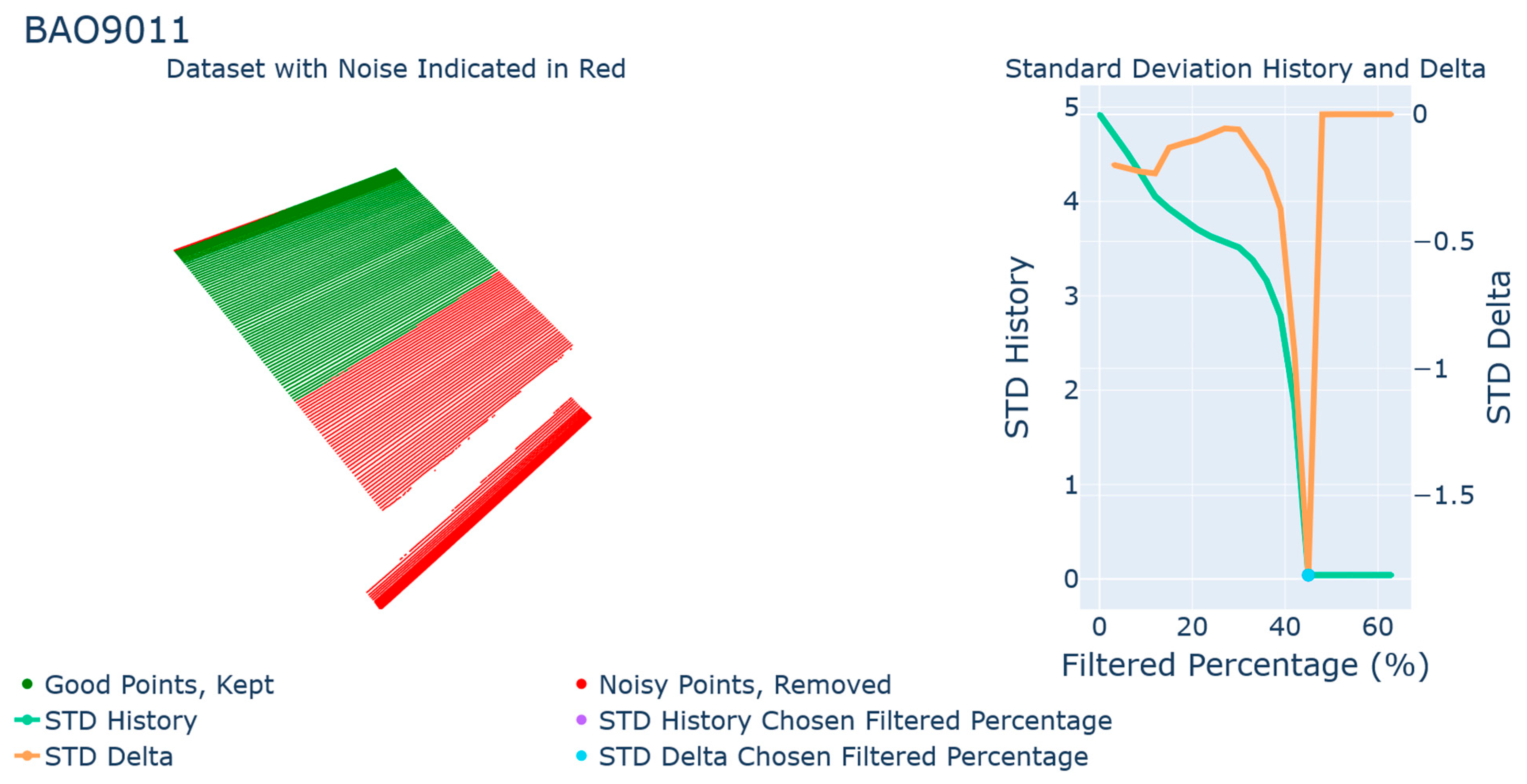
Finally, the SLS part after a 90° turn, at −10° while overexposed (
Figure 12). This data set was quite noisy and contained a “ghost” layer of data below the actual surface. This is possibly due to the light absorption properties of the material. As the laser light hits the surface, it is diffused throughout the surface, causing a “glow”. The scanner’s receiver could still pick this refracted light up, resulting in a surface below the actual surface. This added layer of data caused a shift in the STD delta graph. There are not two linear sections; instead, the line has steps in it after the initial steep increase. Due to the algorithm only using a section from either end of the STD delta graph to determine the intersection point, shown in red in the ideal STD delta graph from
Figure 4, the steps are not considered when determining the correct percentage of data to remove. This allowed most real data to remain while removing most of the noise. The STD of deviation was 0.823 mm which was reduced by filtration to 0.525 mm. The total deviation zone was estimated as 0.734 mm.
Table 1 shows the overall results for each part to four significant digits, due to the number of points used and the accuracy of the used scanner. Regardless of the sample or scan angle, there was a decrease in the detected flatness, showing removal of noise. In the naming of the cases, BA stands for brushed aluminum, GB stands for gauge block, and SLS stands for the selective laser sintered part. The number 90 in the name indicates that this part is rotated 90 degrees for the second set of measurements. The overexposed and underexposed items are defined with the letters “O” and “U” respectively, at the end of each name in this table. Generally, the overexposed condition benefitted the most from noise reduction, likely due to the added light allowed into the receiver causing more noise to be recorded. Conversely, the underexposed condition did not see as great a benefit as less light is allowed into the receiver.
5. Behavior Analysis
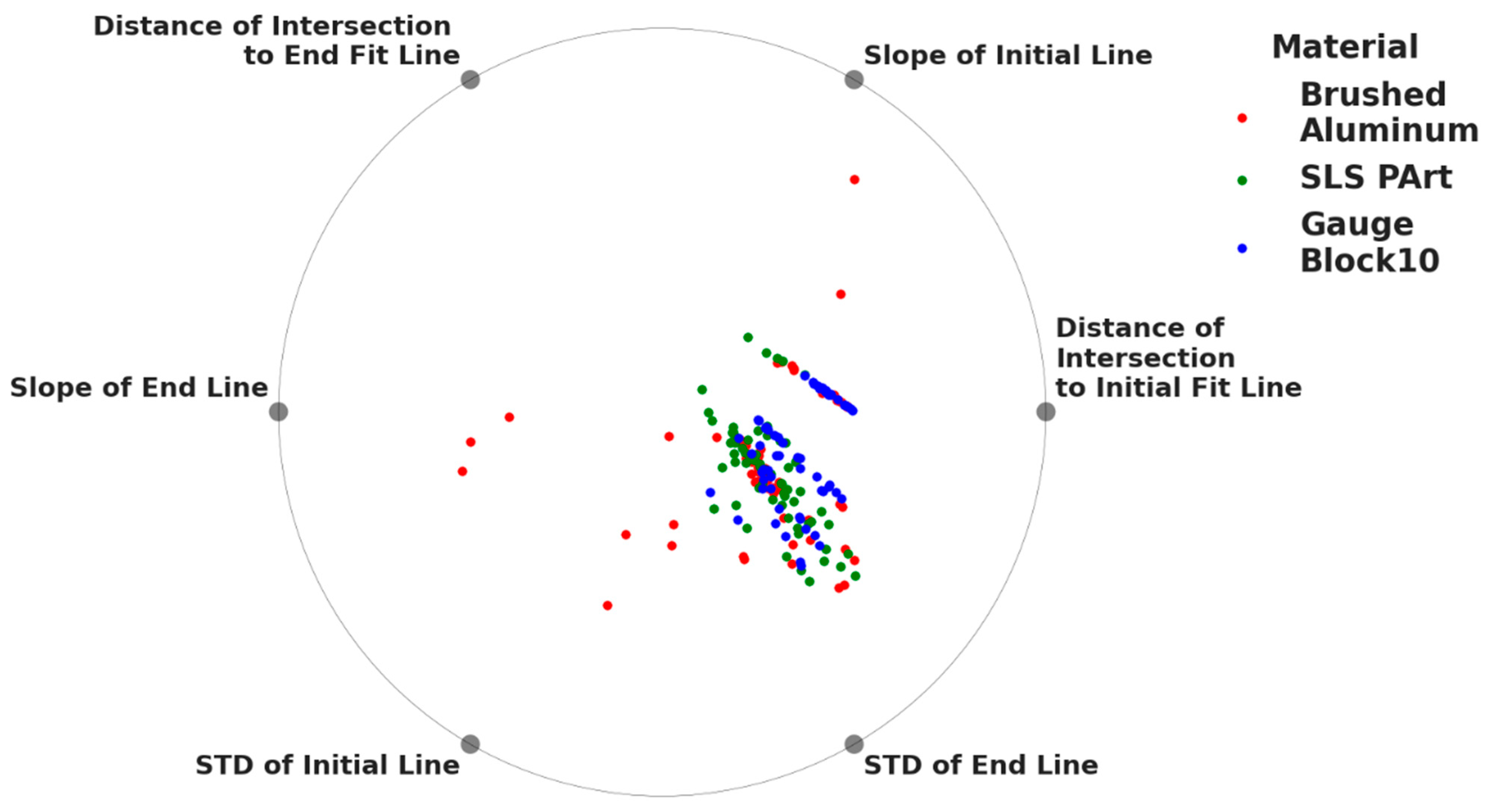
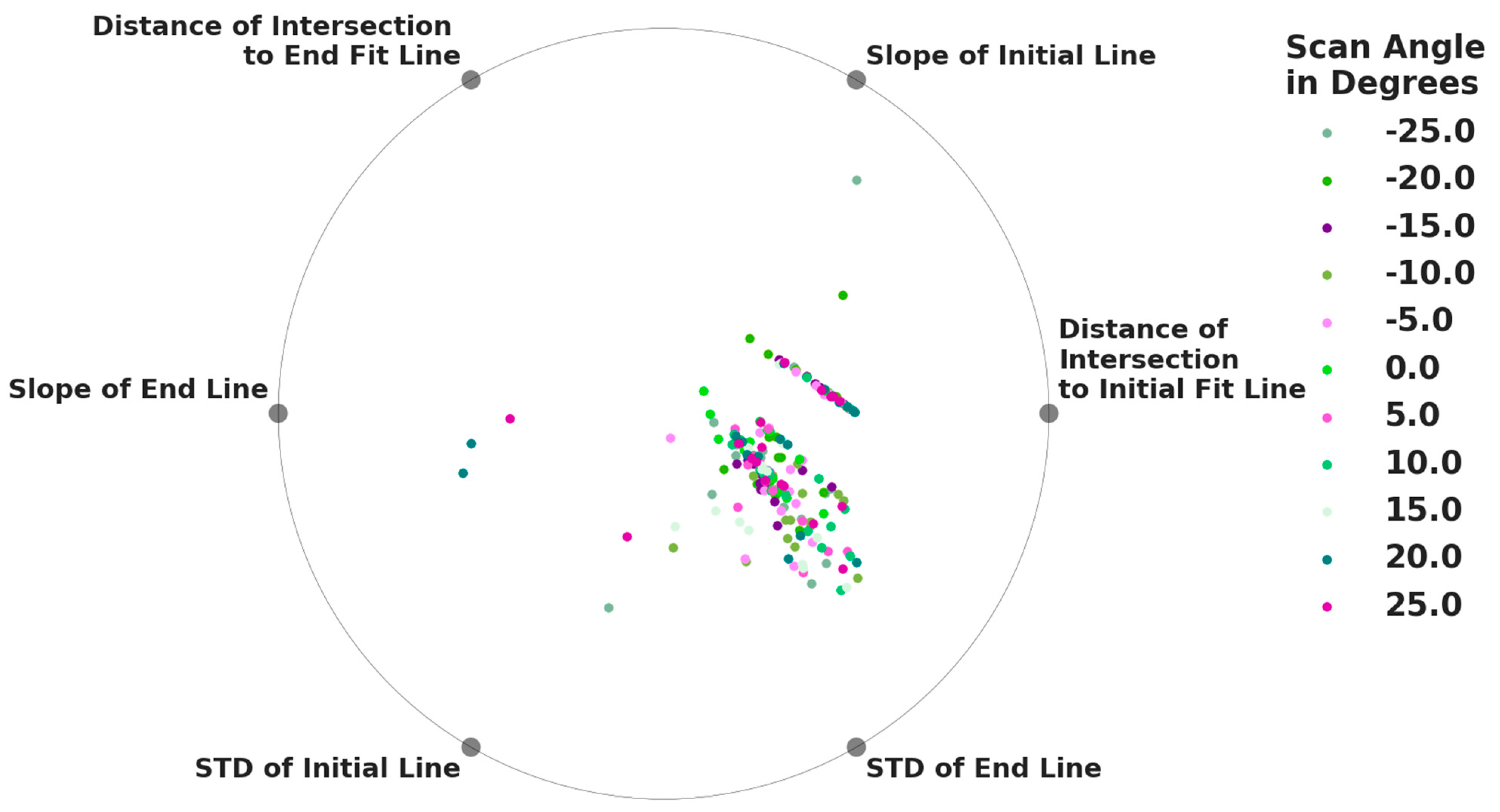
In order to determine how effective the developed methodology is, it is important to study how it is successful to determine the behavior of data. In order to do this, different quantitative parameters for effectiveness were determined. These were determined based on the ideal shape of the STD delta graph. As the graph ideally was comprised of two linear sections, with the intersection of these sections determining the amount of data to remove, parameters evaluating the closeness of this model were chosen. These six parameters are the slopes of the two fit lines, the distance of the chosen filtered percentage and the fit lines, and finally the standard deviation of the Euclidean distance of the sample points to the fit lines. In the ideal situation, the slope parameters will be maximum for the initial line, and 0 for the end line, the distances will both be 0, and the STD values will also both be 0. The following
Figure 13 and
Figure 14 show a RadViz for the test results, to determine the similarities in the parameters for each material and angle tested. RadViz is a multivariate visualization algorithm that allows for different variables to sit along the outside of a circle, where inside the circle different datapoints, for this purpose test cases, are placed. These data points are pulled to each of the outer variables as though attached by a spring and using the value of the variable as a spring constant, the datapoint is placed where the force would be equal to zero [
38]. This method can be useful to determine if your data clusters well, or if there is excessive variation within your data set.
In these visualizations, clear clustering can be seen. In this visualization, clustering is indicative of the correlation between different parameters. If for multiple, or many tests, the results cluster to one section of the circle, the items closest have the greatest effect on the result of the test. For all but the outliers, there was a very clear pull to both the distance of intersection to the initial line fit and to the STD of the end line. This means these two parameters likely have the greatest effect on the result of this filtering method and can be used to judge if a particular set of parameters for a particular work piece is optimal. For both the SLS Part and gauge block, the results were all very closely clustered together. These parts did not have the extreme reflectivity of the brushed aluminum piece, and so the results are very closely correlated. For the brushed aluminum sample, the test results outside of the cluster area all correspond to extreme angles of a scan. This is likely due to the extreme angle of the scan and the high reflectivity of the material causing only a small amount of light to enter the receiver. In this case, filtering is not an effective strategy as the data collected will be inherently wrong. To fix these cases, different scanning parameters would need to be chosen entirely. However, in most cases, the tight clustering shows that the filtering scheme is effective, even at extreme angles, for two of the three surfaces tested, and for non-extreme angles for the brushed aluminum sample.
6. Conclusions
In this paper, a noise reduction algorithm for planar systems was introduced. This system examined datasets globally in order to remove noisy data points from 3D point cloud datasets using a statistics-based approach. The methodology and algorithm were introduced and explained, and three sample parts were measured using a detailed procedure by robotic laser scanner 33 times under various conditions, for a total of 198 scans. These datasets were then processed using the algorithm in order to determine if the noise reduction was effective. Overall, the results are highly satisfactory and in the majority of cases, only with automatic filtration of a small amount of data, the estimated deviation zones are significantly improved. Examples of these cases are provided in the paper. In datasets where there was a large amount of noise, the algorithm was very effective at minimizing the effect of noise on the results. However, when the data set was already noise-free, the algorithm tended to slightly overcompensate and remove actual data. There are rare problematic datasets that are severely affected by the environmental scanning condition. As a result, a group of false data were introduced in these cases which challenged the algorithm in its filtration process. A few worst cases of these kinds are also presented in the paper. An example can be the cases where the background data was left in the scan, the fit plane was at an angle with the actual surface and so some real data was removed during the filtration process. Regardless of the error, there was evidence of these issues existing in both the STD delta and STD history graphs. It has been demonstrated that the algorithm was fairly successful to filter the false data even in these problematic cases. However, since the false data already form some patterns in these cases, the recommendation is the remove the false data by employing a pattern recognition method prior to using the developed noise filtration algorithm. In general, the developed algorithm and methodology are evaluated to be very efficient in removing the noisiness in optical metrology data. The methodology can also be employed in various scales of data and for various industrial applications. It is computationally very efficient and can be easily used for on-line noise removal during the inspection process.


