1. Introduction
Companies need to adapt continually. Organizations that identify and react with greater agility and intelligence have an advantage in the business environment [
1]. This paper is an expanded version of a previous work [
2] (© 2021 IEEE. Reprinted, with permission, from 14th IEEE International Conference on Industry Applications (INDUSCON)). Advanced digitization within factories, aggregated with Internet technologies and smart devices, seems to change the fundamental paradigm in industrial production [
3]. Some companies are capturing artificial intelligence (AI) application value at the corporate level and many others are increasing their revenues and reducing costs at least at the functional level [
1,
4,
5]. The most-reported increase of revenues is for inventory and parts optimization, pricing, analysis of customer-services, sales and forecasting [
1].
According to a study published by Massachusetts Institute of Technology (MIT) Sloan Management Review in collaboration with Boston Consulting Group [
6], almost 60% of respondents on a global survey of more than 3000 managers assert that their companies are employing AI, and 70% know the business value proportioned with AI applications. Notwithstanding the evidence, only 1 in 10 companies achieve financial benefits with AI. The survey found that organizations apply basic AI concepts, and even with adequate data and technology, financial returns are minimal. Companies need to learn from AI and implement organizational learning, adapting their strategies over time. Hence, their chances of generating financial benefits increase to 73% [
6].
A study compared the main trends in the digitization present in a “Factory of the Future” [
7], showing that a digital factory has the goal to automate and digitize the intra-factory level, using virtual and augmented reality, and simulations, aiming to optimize production. The study reports that at the lowest layer of the supply chain, the Internet of Things plays an important role in the paradigms of real-time analysis, smart sensing, and perception. From the perspective of an inter-factory collaboration, the trends are related to cloud manufacturing and virtual factory. Big data is been used to support production, to help in internal business, and to guide new discoveries [
8].
Technology implies accurate processes, better tools, and business innovation. It is compelling to blend automation, computer vision, and deep learning (DL) to improve warehouse management. Modular solutions, embedded intelligence, and data collection technologies are the key points to flexible automated warehouses [
9]. Amazon invested heavily in drive units, picking robots, autonomous delivery vehicles, and programs to help workers learn software engineering and machine learning skills [
10]. Researches conducted on literature show that in the last decade several studies on the theory of inventory management improvements were developed and new technologies could be applied in warehouse management systems [
11]. In addition, over the last ten years, Artificial Intelligence played an important role in the supply chain management field, with customer demand predictions, order fulfillment, and picking goods. Nonetheless, it is reported a lack of study on the warehouse receiving stage [
11]. According to an exploratory study, the implementation of warehouse management systems can bring benefits related to increasing inventory accuracy, turnaround time, throughput, workload management, productivity, besides reducing labor cost and paperwork [
12]. In a proposed architecture for virtualization of data in warehouses, the authors replace conventional data with a non-subjective, consistent, and time-variant type of data, making a synthetic warehouse for analytical processing, aiming scalability and source dynamics [
13]. Radiofrequency identification, short-term scheduling and online monitoring are largely used in warehouses and industry [
14,
15,
16].
In this scenario, a Brazilian electrical company is facing obstacles in its logistics. The main problems that demand solutions are the outlays of inventory control, the time-consuming tasks, and the lack of reliability in maintaining a manual flow. There is a burgeoning need for automated processes in order to reduce costs. The identification of products in this company’s warehouse is the flagship of a project to automate flow control and inventory. By this means, it is essential to build an intelligent application that can classify the products. In order to handle a classification task for this project, a real dataset was created. The dataset building represents a challenge given the variety of steps. Therefore, they were required hours of shooting, labeling, and filtering data process. Consequently, the project seeks to develop an intelligent system capable of assisting in the organization and management of the inventory of a company in the energy sector, an automated solution that checks the disposal of items in the warehouse and controls the flow of inputs and outputs, involving applications of computer vision, deep learning, optimization techniques, and autonomous robots. As part of the project, it is intended to build a tool to classify inventory items. This tool will be encapsulated in the automated system.
A blend of pipelines for colored and depth images is proposed, in a soft voting type of ensemble approach. Each pipeline corresponds to a classifier, and two CNN models are used for this task. The final classification of a scene is performed by this ensemble, not explored for this application yet. The decision is the average of the probabilities of each CNN multiplied by equal weights, meaning that the models have the same influence on the final result.
The remainder of this article is structured as follows.
Section 2 presents the problem description, illustrating the electrical utility warehouse, devices, and sensors applied to capture the images.
Section 3 depicts the dataset developed for this application, which is divided into synthetic and real data. Then,
Section 4 brings the image processing, explaining the selection and the control of captured images during the data gathering step.
Section 5 explains deep learning methods and their hyperparameter tuning to meet the requirements of the project. In
Section 6 the ensemble learning approach is illustrated, followed by
Section 7 illustrates the methodology to assess the different datasets. The results are presented and discussed in
Section 8. Finally,
Section 9 describes the conclusion and future works.
2. Problem Description
The electrical utility warehouse of this company is an 11,000 square meters building, containing more than 3000 types of objects used in the electrical maintenance field. The objects are distributed on shelves across the entire facility. There are a total of twenty-four shelves of 5 m tall, 3 m wide, and 36 m long across the entire building. The company has a constant flow and cannot allow absences of material. The stock needs to be up to date to deliver a reliable and fast service. Therefore, the company is facing management problems that need to be solved: miscounting, time-consuming processes of flow control, inventory check, as well as the costs of such processes. The project aims to reduce the impact of these issues, combining new technology and intelligent solutions, improving inventory management. Thus, an automated inventory check is proposed, using artificial intelligence, computer vision, and automation.
With the aim of keeping the inventory up to date, the project foresees two different procedures: flow control and periodic verification. The first procedure is designed to check every item that enters or leaves the warehouse using gateways and conveyor belts. Large objects will be handled by electric stackers, while small ones will be manually placed in the conveyor belts. To verify the handling products, gateways and conveyor belts will be equipped with cameras. The second procedure consists of an Automated Guided Vehicle (AGV) that checks all shelves inside the warehouse, counting the number of items.
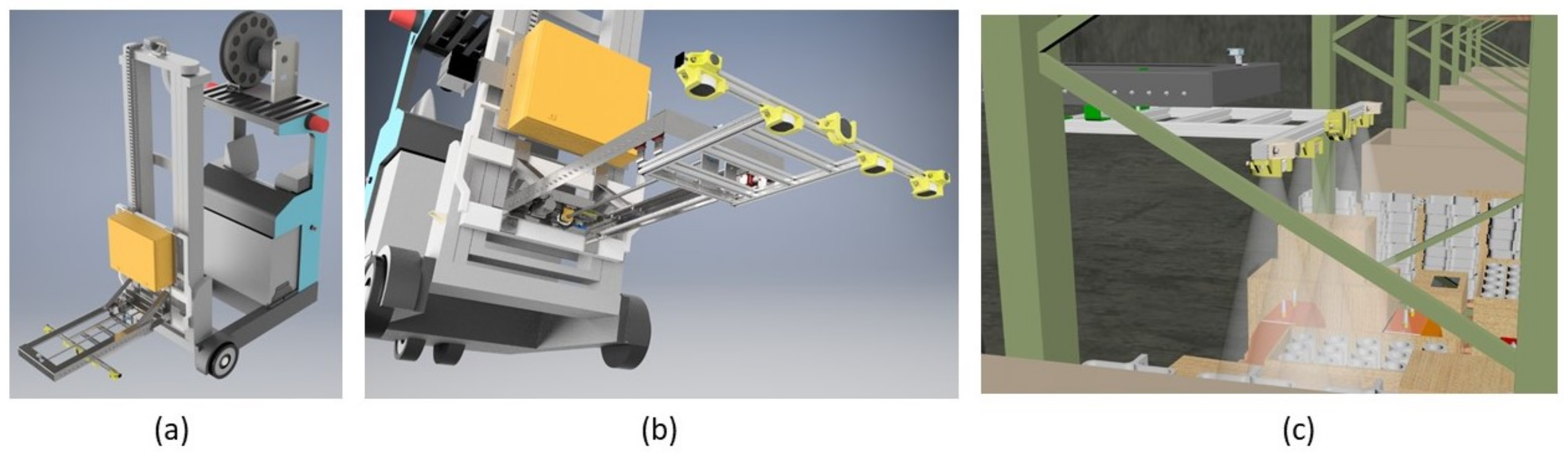
The AGV is a Paletrans PR1770 electric stacker that will be fully automated in order to work remotely and to take pictures of the products. The AGV will receive a retractable robotic arm with 5 cameras, one in the front of the arm and the others in a straight-line arrangement, enabling a better field of view and capturing the full dimension of the shelves.
Figure 1 (a) shows an overview of the AGV with the robotic arm.
Figure 1 (b) represents the robotic arm fully extended and Light Detection and Ranging (LiDAR) positions. Finally,
Figure 1 (c) illustrates the AGV capturing images of the shelves.
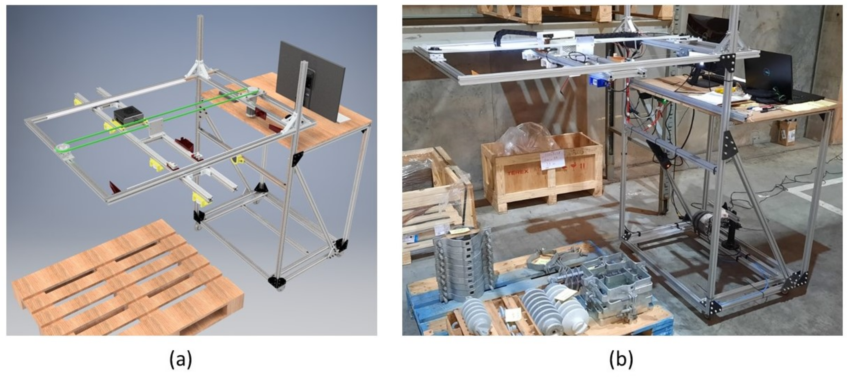
Since the gateways, conveyor belts, and the AGV are still in development, a mechanical device was built to manually capture the images inside the warehouse. The device was designed to emulate the AGV and it is manually placed on the shelves. Consequently, it was possible to build a dataset of products before the project conclusion. The data acquisition allows studying and developing techniques of image classification.
Figure 2 (a) shows the project and (b) the constructed mechanical device.
The device is a mechanical structure equipped with the same technology that will be used in the AGV, gateways, and the conveyor belts: Intel RealSense L515 LiDAR cameras with laser scanning technology, a depth resolution of 1024 × 768 at 30 fps, and a Red–Green–Blue (RGB) resolution of 1920 × 1080 at 30 fps. They are arranged identically as in the AGV design shown in
Figure 1. The technology embedded in the mechanical device for the data acquisition is described as follows: a portable computer with Ubuntu, five L515 cameras, a Python script with OpenCV, Intel Librealsense and Numpy libraries, an uninterruptible power supply (UPS) device for power autonomy, and a led strip for lighting control.
The warehouse harbors mainly materials for maintenance services for electrical distribution systems. Switches, contactors, utility pole clamps and brace bands, mechanical parts, screws, nuts, washers, insulators, distribution transformers, and wires are stored in the warehouse, among other products.
One of the essential parts of this project is to build a tool that classifies the products inside the warehouse using deep learning techniques. This tool analyzes the quality of captured images and classifies the objects placed on the shelves by RGB and Red–Green–Blue-Depth (RGB-D) data. The warehouse is considered an uncontrolled environment, increasing the difficulties for a computer vision application. It means that the shelves and pallets do not have a default background, like in some computer vision competitions. Moreover, at the time of the dataset building, there were no rules applied related to the arrangement of materials. There are issues that will be faced in order to accomplish this task, such as this random displacement of products. Moreover, the warehouse presents difficulties related to lighting distribution. Some places have poor lighting conditions. The LED strip installed on the AGV provides a better distribution of light in the shelves that has no sufficient conditions for data collection.
The depth information provided from the LiDAR can be used in order to extract more features of the scenes, where sometimes colored images do not hold these features. The arrangement of the five cameras has the role to avoid problems related to occlusion. The straight line of four cameras facing down is a setup that was brought to maximize the field of view of the scene. The robotic arm will slide from the beginning to the end of each pallet, allowing cameras to capture the most information possible for this arrangement. The frontal camera setup was also designed to give another perspective of the scene, taking pictures from the front of the pallets. Some objects are stored partially occluded. These objects are, for instance, insulators inside wooden boxes. This is a challenge that needs to be addressed as well.
3. Image Processing
The image processing operation for the captured images is divided into two parts. First, the quality of the images is checked, and then, two histogram analyses are performed. If the captured colored image is not satisfactory according to the procedure described in this section, the RGB and RGB-D images are discarded and another acquisition is made.
3.1. Image Quality Assessment
The image quality assessment (IQA) algorithms examine any image and generate a quality score on its output. The performance of these models is measured based on subjective human quality judgments, since the human being is the final receiver of the visual signal, as mentioned in [
17]. Additionally, IQAs can be of three types, such as full reference (FR), reduced reference (RR), and no-reference (NR) [
18]. The FR type is where an image without distortion (reference) is compared with its distorted image. This measure is generally applied in the evaluation of the quality of image compression algorithms. Another possibility is RR, without a reference image, but an image with some selective information about it. Finally, NR (or blind object) is the type where the only input from the algorithm is an image whose quality is to be checked [
19].
In this research, an NR IQA algorithm called blind/referenceless image spatial quality evaluator (BRISQUE) [
17] was applied, in order to evaluate the quality of the images at the time of mechanical device acquisition. The BRISQUE algorithm is a low complexity model since it uses only pixels to calculate features, with no need to perform image transformations. Based on natural scene statistics (NSS), which considers the normalized pixel intensity distribution, the algorithm identifies the unnatural or distorted images considering if they do not follow a Gaussian distribution (Bell Curve). Then, a comparison is made between the pixels and their neighbors by pairwise products. After a feature extraction step, the dataset feeds a learning algorithm that performs image quality score predictions. In this case, the model used was a support vector regressor (SVR) [
17].
The objective is to have an image quality control at the time of stock monitoring. In this scenario, the main problem is the brightness of the environment. Therefore, in addition to the assessment value of the algorithm, an analysis of the distribution of the image histogram is performed. Thus, 25 images captured were evaluated, which cover the most diverse histogram distributions, seeking to define the limits of the mean of the histogram distribution and the quality limit value. Based on the subjective judgments of the project’s developers, the threshold for the quality score of the images was set at 30, with the scale of the algorithm varying from 0 (best) to 100 (worst). Hence, images with an IQA score below 30 are considered acceptable. If the value is higher, the system considers the image unsatisfactory.
3.2. Image Adjustment
During this step, an analysis of image histogram distribution is performed to verify if there is a lack or excess of exposure. According to the evaluation of the images, the acceptable limits for the distribution of the histograms of the images were defined between 75 and 180, being a scale of 0 to 255 levels of gray. When the value is less than 75, it is a poor light environment. On the other hand, a result higher than 180 means light in excess.
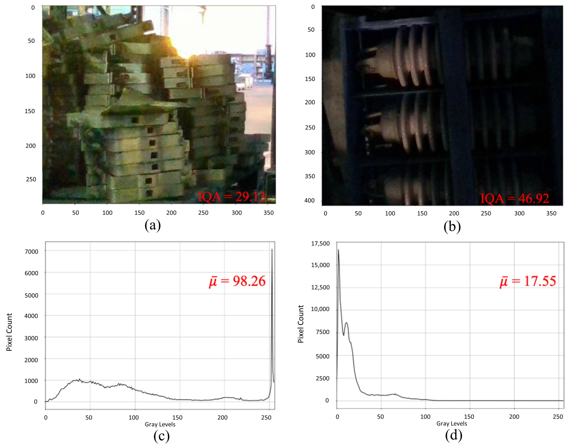
An example is shown in
Figure 3, where two images are presented with different IQA values and their respective average of gray levels for each histogram.
Figure 3 (a) has the best quality according to the BRISQUE algorithm. Analyzing its histogram in (c), the mean value (
) was 98.26. According to this assessment, the image is considered acceptable to provide information about the location. However,
Figure 3 (b) had an IQA value higher than the limit of 30, being unsatisfactory for the classification of the algorithm. In this case, the mean of the histogram is analyzed, where it is identified that the image problem is of low exposure since the mean values were less than 75, as shown in (d).
If the images are rejected by the assessment analysis, luminosity correction is carried out by adjusting the intensity of the light-emitting diodes (LEDs) present in the AGV structure. If after three consecutive attempts it is not possible to obtain an acceptable image in consonance with the defined parameters, the vehicle system registers that it was unable to collect data from that location and recommends the manual acquisition of images/information. Thus, an employee must go to the site and check the content of that pallet. The disadvantage of a manual check is that it goes against the main objectives of automated inventory control. Besides the time misspending by an employee, performing a manual verification, there is a time to register it in the system. During this period, the inventory will not be updated correctly.
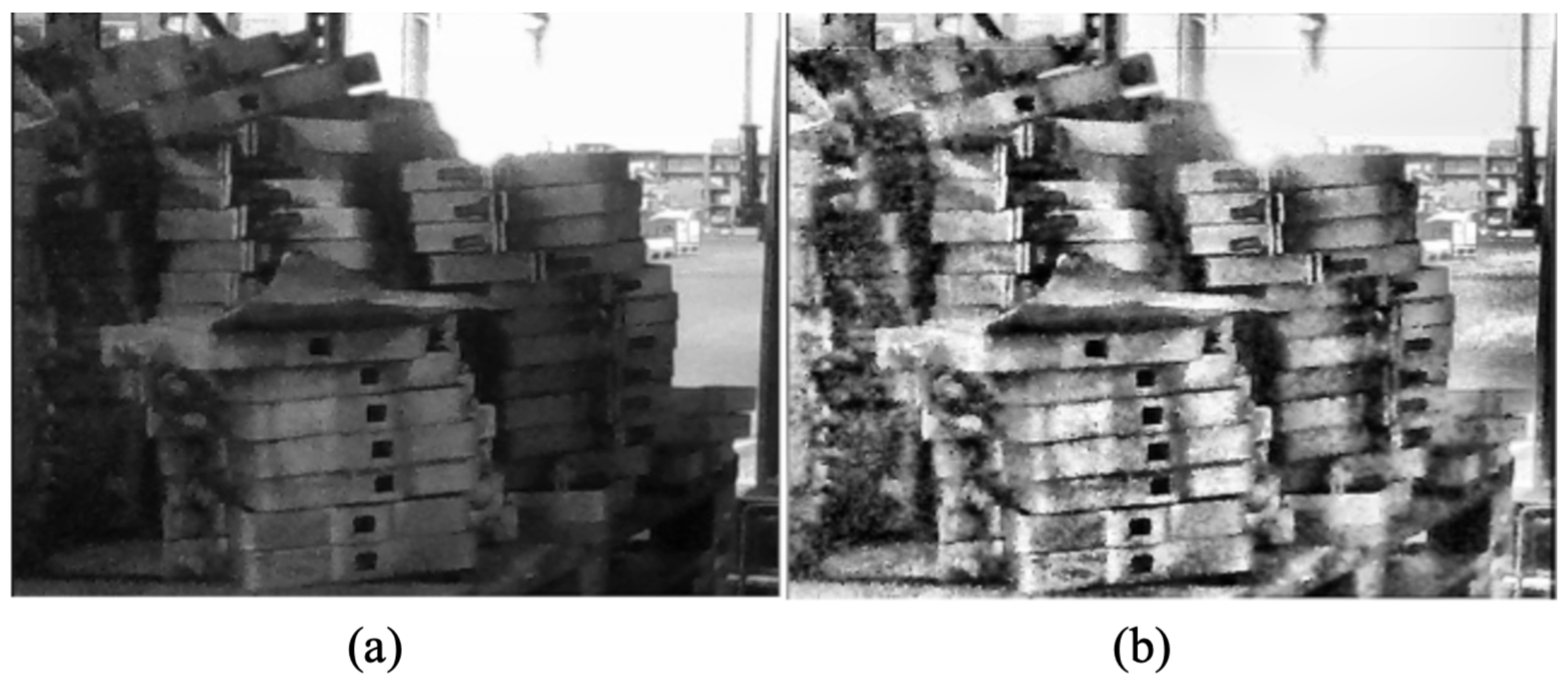
Finally, if an image is considered valid using BRISQUE and histogram analysis criteria, then a new histogram analysis is performed, looking for the values that appear most frequently (peaks). Hence, if there are peaks close to the extremes, in a range of 20 levels on each side (0 represents black and 255 white color), an adaptive histogram equalization (AHE) [
20,
21] is performed in order to improve regions of the image that have problems with luminosity. Analyzing the histogram of the first image in
Figure 3 (c), there is a peak close to the 255 level. Performing an AHE, the image will present a better distribution of the gray levels, providing an enhanced description of its characteristics to the neural network. The result is shown in
Figure 4, where (a) indicates the original image and (b) the image after the AHE process.
4. Synthetic and Real Data
Commonly, the use of deep learning techniques to deal with classification problems requires a great amount of data [
22]. However, if there are not sufficient images on the dataset, the deep learning models might not be able to learn from the data. One way to solve this issue is to apply data augmentation processing, which is divided into two categories: classic and deep learning data augmentation. The classic or basic methods are flipping, rotation, shearing, cropping, translation, color space shifting, image filters, noise, and random erasing. Deep learning data augmentation techniques are Generative Adversarial Networks (GANs), Neural Style Transfer, and Meta Metric Learning [
23]. Moreover, 3D Computer-aided design (CAD) software and renders are useful for generating synthetic images to train algorithms to perform object recognition [
24]. Game engines are great tools to build datasets as well [
22,
25].
Another point is that manually labeling a dataset requires a great human effort and it has an expensive cost [
25]. In contrast, on synthetic datasets, the process of labeling can be done automatically and it is easier to achieve more variations [
26]. In addition, there are some situations where the creation of a dataset is critical or new samples acquisition are rare, and therefore, the synthetic approach can balance these problems, as presented in critical road situations [
27], volcano deformation [
28], radiographic X-ray images [
29] and top view images of cars [
30].
The use of generated images is not exclusively done by critical datasets. This method is used in applications of common activities and places as well. For instance, in a method that places products on synthetic backgrounds of shelves on a grocery object localization task [
31], detection of pedestrian [
25,
27], cyclists [
32], vehicles [
26] and breast cancer [
33], classification of birds and aerial vehicles [
22], and synthetic Magnetic Resonance Imaging (MRI) [
34]. However, generated images sometimes present a lack of realism, making models trained on synthetic data perform poorly on real images [
24].
For this reason, there are some methods of using synthetic data during the training step of a deep learning model. The first one is training and validating only on the synthetic domain, and testing on real data. As reported by Ciampi et al. [
25] when the model is trained only on synthetic, it shows a performance drop. In contrast, Saleh et al. [
32] point out the ability to generalize their framework by training with synthetic data and testing on the real domain, increasing 21% the average precision in comparison with classical object localization methods. In Öztürk et al. [
22], they demonstrated that models trained on synthetic images can be tested on real images in the task of classification.
The second method consists in mixing both domains when training the model, and testing on real images [
27]. Reference Anantrasirichai et al. [
28] presented that the training process with synthetic and real data improved the ability of the network to detect volcano deformation. The third method is the use of a transfer learning approach to mitigate the difference between synthetic and real domain shifts. The CNN models are trained on synthetic domain and fine-tuned on real dataset [
26]. In an approach based on convolutional neural networks for MRI application, Moya-Sáez et al. [
34] proved that fine-tuning a model trained with synthetic data improved performance, while a model trained only with an actual small dataset showed degradation. Reference Ciampi et al. [
25] explored methods two and three to mitigate the domain shift problem, mixing synthetic and real data and training the CNN on a synthetic dataset, and fine-tuning on real images on training step. Both adaptations improved performance on specific real-world scenarios. Some techniques adapt CAD to real images, like the use of transfer learning to perform a domain adaptation loss, aligning both domains in feature space [
24].
When working with 3D images, Talukdar et al. [
35] evaluated different strategies to generate and improve synthetic data for detection of packed food, achieving an overall improvement of more than 40% on Mean Average Precision (mAP) object detection. The authors used the 3D rendering software Blender-Python. These strategies are a random packing of objects, data with distractor objects, scaling, rotation, and vertical stacking.
In this project, to generate the synthetic dataset, Blender [
36] by Blender Foundation was selected for being an open-source software that provides a large python API [
37] to create scenes for rendering. Moreover, Blender provides physically based rendering (PBR) shaders, getting the best out of its engines, Cycles, and Eevee, respectively a ray tracing and rasterization engine. A ray-tracing engine computes each ray of light that travels from a source and bounces throughout the scene and a rasterization engine is a computational approximation of how light interacts with the materials of the objects in the scene [
38].
A nice synthetic dataset of rendered images must approximate real-world conditions, so the best choice is to use the Cycles engine for its ray tracing capability as mentioned by Denninger et al. [
39] compared to rasterization engines because shading and light interaction is not consistent. Nonetheless, this method is computationally expensive considering the complexity of the scenes to render, number of samples, and resolution, making it difficult to generate large datasets. The Cycles approach is more accurate [
38]. However, Eevee was chosen for rendering due to its Physically Based Rendering (PBR) capabilities differentiating from other rasterization engines, being the best choice when taking into account quality and speed.
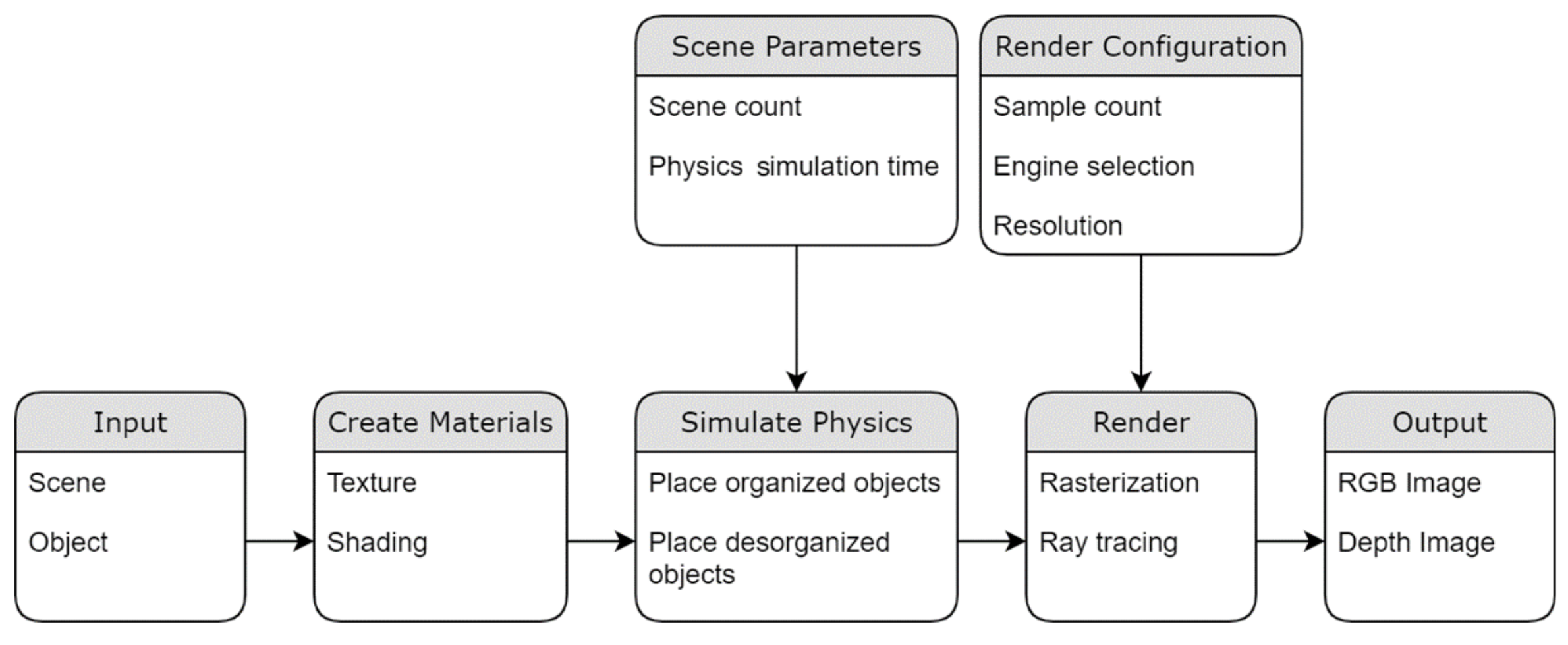
The scene was created with Blender’s graphic interface, setting the base to receive objects in a single blend file. Blender’s python API [
37] was used to create the pipeline, as shown in
Figure 5, to configure intrinsic parameters of the real camera that was used to take real-world photos, to choose objects, to simulate physics to place then randomly, to create or set shades for materials and to prepare post-processing and generate depth images based on the rendered scene.
This way the pipeline could be executed in a loop, considering the parameters scene count number, in an autonomous form to randomize the scenes and create a large dataset of synthetic RGB and depth images separated by objects classes to be used in training and test.
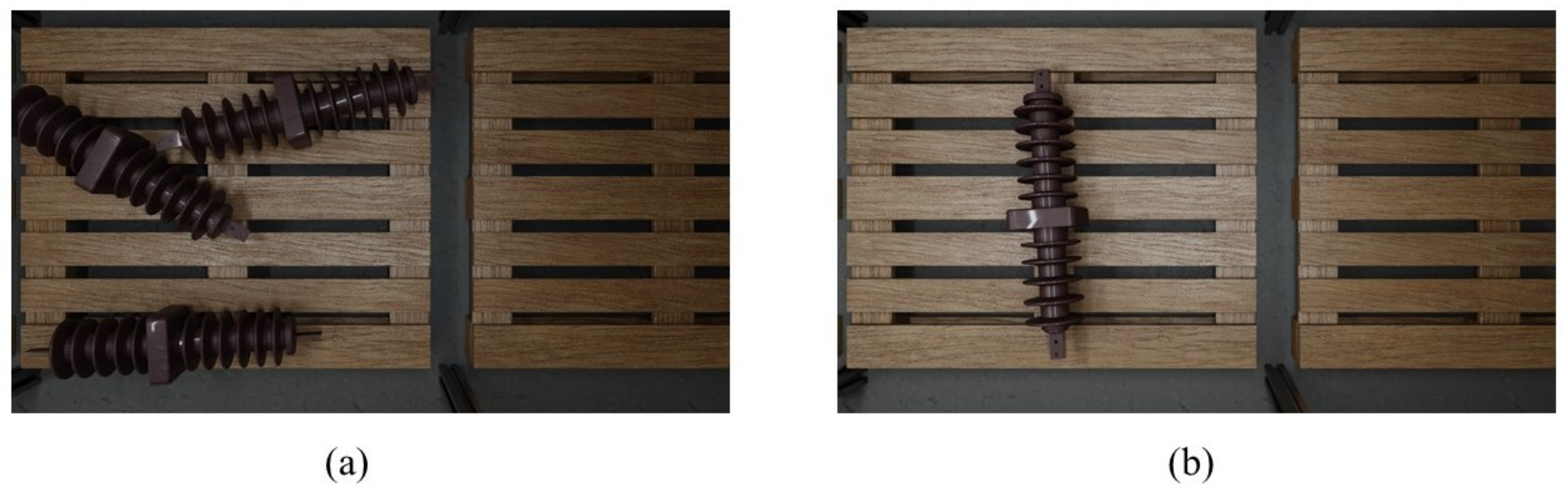
As a comparison, a test was conducted by rendering a scene with 5 cameras and 7 camera positions, giving a total of 35 rendered images for each engine, as shown in
Figure 6. Cycles (a) took approximately 19.99 s to render one image and 759.2316 s to render all images. Eevee (b) took 2.97 s on one image and 140.3429 s to generate all images. Whileough with different light sets, object positions, and quantity due to randomization, the overall shading of both engines got the same look as the materials are processed the same way. However, Cycles can create better shadows and reflection as light rays interact with all objects, in exchange for render speed.
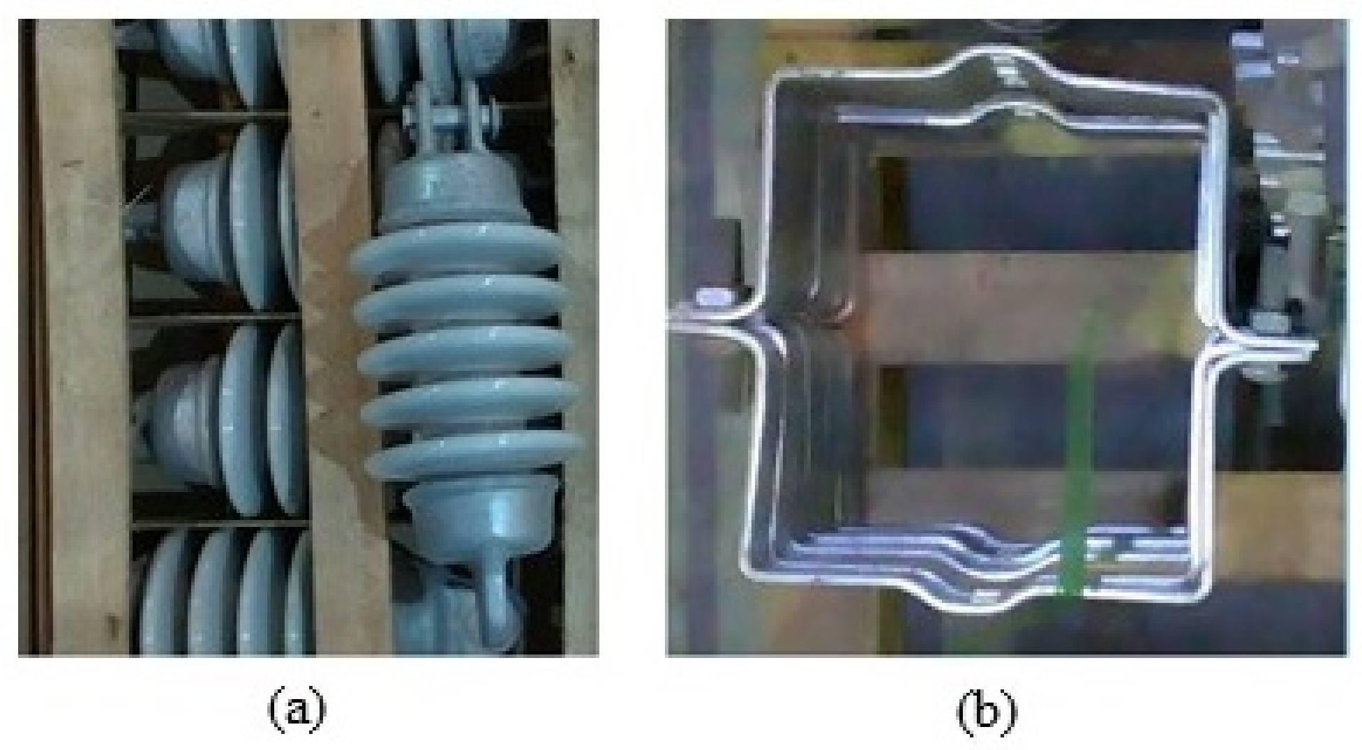
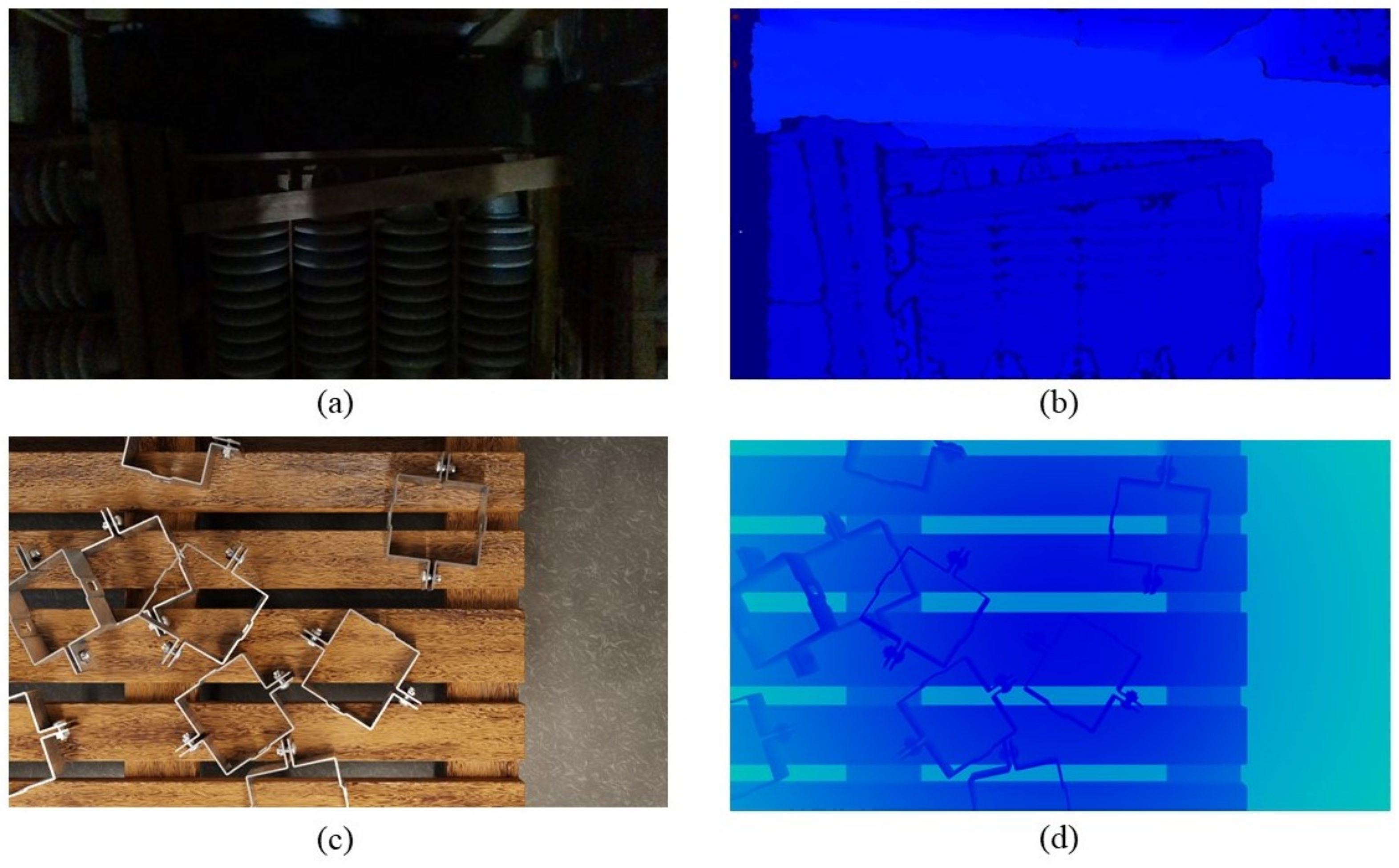
To create the real dataset, an acquisition took place inside the warehouse using the mechanical device to manually capture the images. Two classes of materials were chosen to compose the dataset, making this a binary problem to be solved. The classes are utility pole insulators in
Figure 7 (a) and brace bands in
Figure 7 (b). These classes are the objects that appear more frequently in the warehouse, and due to their high transport flow, they are stored close to the first shelves to facilitate their flux.
To build the dataset, the mechanical device was allocated on the pallets, performing the data collection, as described in
Section 2. A scene (pallets with a displacement of objects) generated seven RGB and seven RGB-D pictures per camera from the straight line of 4 cameras, and the frontal camera took one picture for each domain. The result is a total of 58 pictures per scene.
The datasets used for these projects are from the synthetic and real domains. According to the literature review presented in this section, the use of synthetic images has improved training and the final accuracy for object classification tasks. However, synthetic data is not robust enough to be used solo in the application. This is the reason why the real data collection approach was also chosen to be included in the project. In this way, real and synthetic data can be applied as input to the deep learning models, to help train and achieve better accuracy in classifying the objects.
5. Convolutional Neural Networks
Deep Learning has been used in areas like computer vision, speech processing, natural language processing, and medical applications. To summarize, deep learning is many classifiers based on linear regression and activation functions [
40]. It uses a high amount of hidden layers to learn and extract features of various levels of information [
41]. Computer vision and convolutional neural networks accomplished what was considered impossible in the last centuries: recognition of faces, vehicles that drive without supervision, self-service supermarket, and intelligent medical solutions [
42]. Computer vision is the ability of computers to understand, taking digital images or videos as input, aiming to represent an artificial system [
40,
43].
CNN is a type of neural network that delivered a promising performance on many competitions of computer vision and captivated the attention of industry and academia over the last years being a feedforward neural network that automatically extracts features using convolution structures [
41,
42,
43,
44,
45,
46,
47]. CNN is a hot topic in image recognition [
40]. Classification of images consists of allocating an image within a class category and CNN generally needs a large amount of data for this learning process.
Some of the advantages of a CNN are local connections, reducing parameters, and making it faster to converge. Moreover, they have a down-sampling dimensionality reduction, holding information while decreasing the amount of data. On the other hand, some challenges and disadvantages are: it may lack in interpretation and explanation; noise on input can cause a drop in performance; the training and validating step requires labeled data; a few changes in its hyperparameters can affect the overall performance; it cannot hold spatial information and they are not sensitive to slight changes in the images. Furthermore, the generalization ability is poor and they do not perform well in crowded scenes. Lastly, training a model requires time and computational cost and updating a trained model is not simple [
40,
42,
43].
Optimization of deep networks is a non-stopped research area [
48] and CNN improvements usually come from a restructuration of processing units and design of blocks related to depth and spatial exploitation [
43]. The following CNN architectures presented great performance, state-of-the-art results, and innovation to this field of study.
5.1. AlexNet
The AlexNet architecture is a well-known CNN and caught the attention of the researchers when it won the ILSVRC-2012 competition by a large difference, achieving a top-5 error rate of 15.3% [
49]. Moreover, one of the most important contributions of the paper was training the model with Graphics Processing Unit (GPU). The use of GPU allowed training deeper models with bigger datasets.
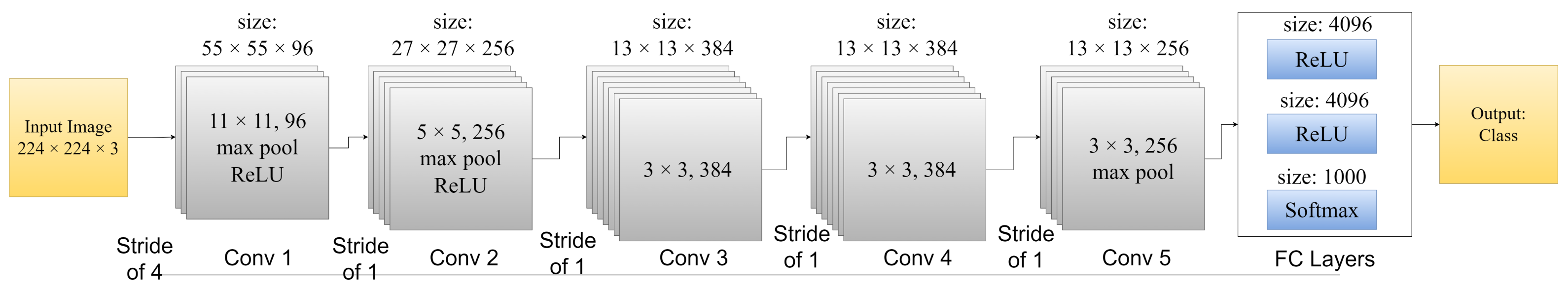
AlexNet is a five convolutional layer network, with three fully connected layers. The softmax is the final layer. The third and last layer is fully connected with a softmax function of 1000 neurons. The AlexNet’s architecture is illustrated in
Figure 8.
The AlexNet architecture [
49] also proposed a local response normalization. To achieve a generalization to the normalization, a function was implemented in between the first three convolutional layers. The activity of a neuron when given a certain kernel
i at the position
x and
y is measured by
.
N is the total of kernels and n represents the number of adjacent kernel maps at the same spatial position. Three constants are used, being
k,
, and
. The term
measures the response normalized activity and follows the Equation (
1)
In the equation, k = 2, n = 5 and = and are hyperparameters determined on validation. Besides the use of GPU, another contribution of the authors in this paper is the use of dropout and data augmentation. The first technique was implemented in all neurons of FC layers 1 and 2. The outputs of the neurons were multiplied by a constant of 0.5.
5.2. VGGNet
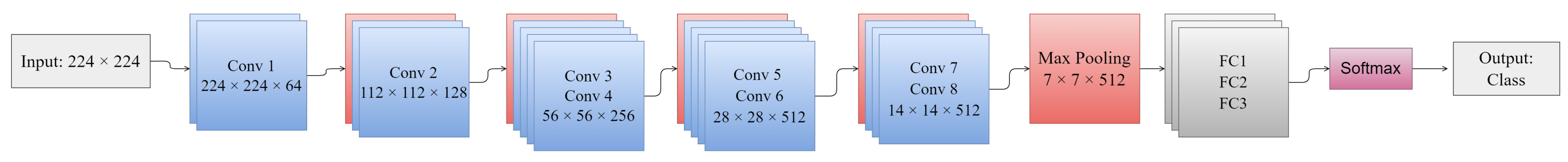
The Visual Geometry Group (VGG) architecture is proposed by Simonyan and Zisserman [
50]. VGG-11 is a network with 8 convolutional layers and 3 FC layers. The network performs a pre-processing on the image, subtracting the average values from the pixels in the training set. The input then goes to several convolutional layers of 3 × 3 filters. The VGG-11 achieved a top-5 test accuracy of 92.7% on ILSVRC.
The authors use five max pooling operations to achieve spatial pooling. This operation has a window of 2 × 2 pixels, using a stride of 2. The number of channels of the network starts with 64 on the first layer and increases the width by 2, ending with 512 channels on the last layer. Then, the last three layers are FC layers. The architecture of VGG-11 can be seen in
Figure 9.
A novelty of VGG in comparison with Alexnet is the use of 3 × 3 convolutions instead of 11 × 11 ones. The authors showed that these new narrow convolutions performed better. For instance, if input and output of the mentioned 3 × 3 operation has
C channels, the parametrization follows Equation (
2), resulting in the number of weights
On the other hand, with the use of just one 7 × 7 convolutional layer, this number of parameters is shown in Equation (
3). As it can be seen, there is an increase of 81% of parameters
VGG-11 has 133 million parameters. To bring more data to train the model, the authors performed a data augmentation on the dataset. This data augmentation helps to train the model, however, it delays the process and requires more computational power.
5.3. Inception
The neural networks proposed by Szegedy et al. [
51] explored the other dimension of neural networks. Inception version 1 ( Inception V1) came to increase the width of the architectures, not only the depth. Mainly, Inception V1 has three different sizes of filters, 1 × 1, 3 × 3, and 5 × 5. The second proposed architecture (Inception V2) reduces its dimensions, adding a one squared convolution just before the mentioned 3 × 3 and 5 × 5 filters from Inception V1. That operation focuses on reducing the parameters of the network, allowing a decrease of computational cost on training.
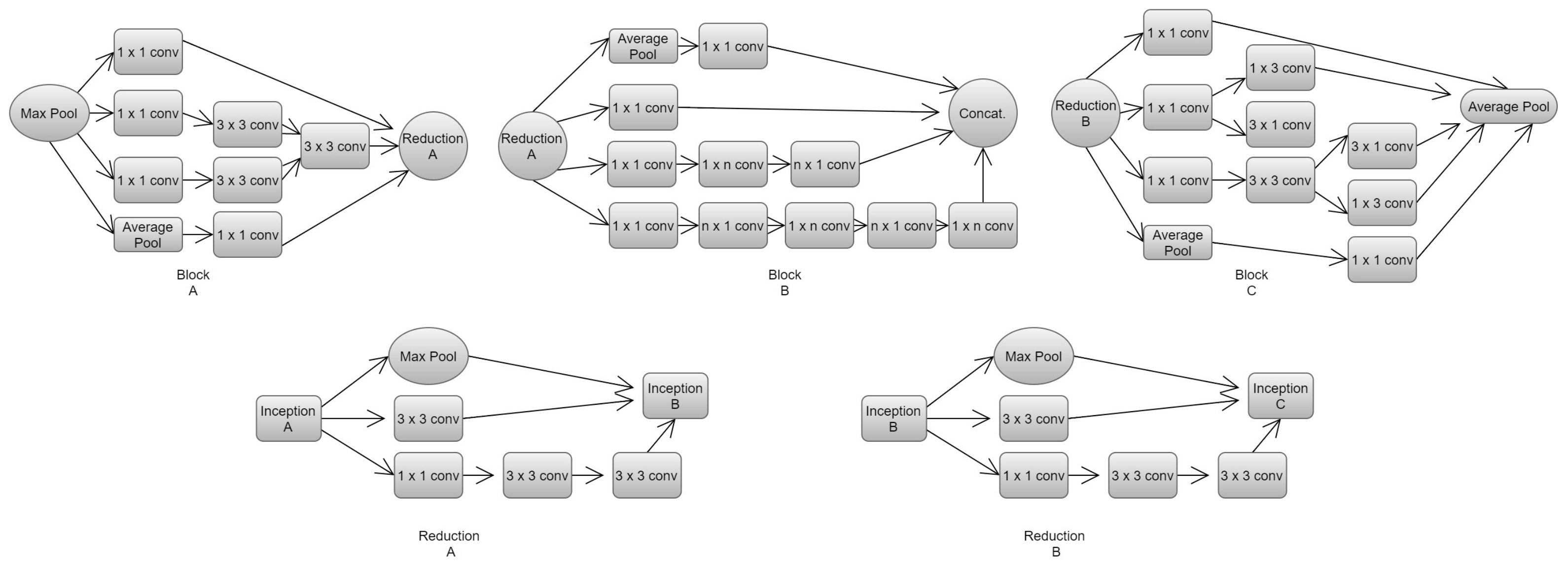
Inception version 3 [
52] proposed a factorization, decreasing the size of convolutions. Two convolutions of 3 squared pixels replace the mentioned 5 × 5 convolutions of previous versions in a block called Block A. The authors implemented a factorization into asymmetric convolutions, changing the 3 × 3 convolution by a 1 × 3 and 3 × 1. Then, one of the 3 × 3 convolutions is replaced by a 3 × 1 and 1 × 3 pixel size, known as Block C. Following the same principle of factorization, Block B is composed of a 1 × 7 convolution, a 7 × 1 in parallel with two 7 × 1 and 1 × 7 convolutions. These blocks are represented in
Figure 10, as well as their respective reduction blocks, where n is set with the value of 7.
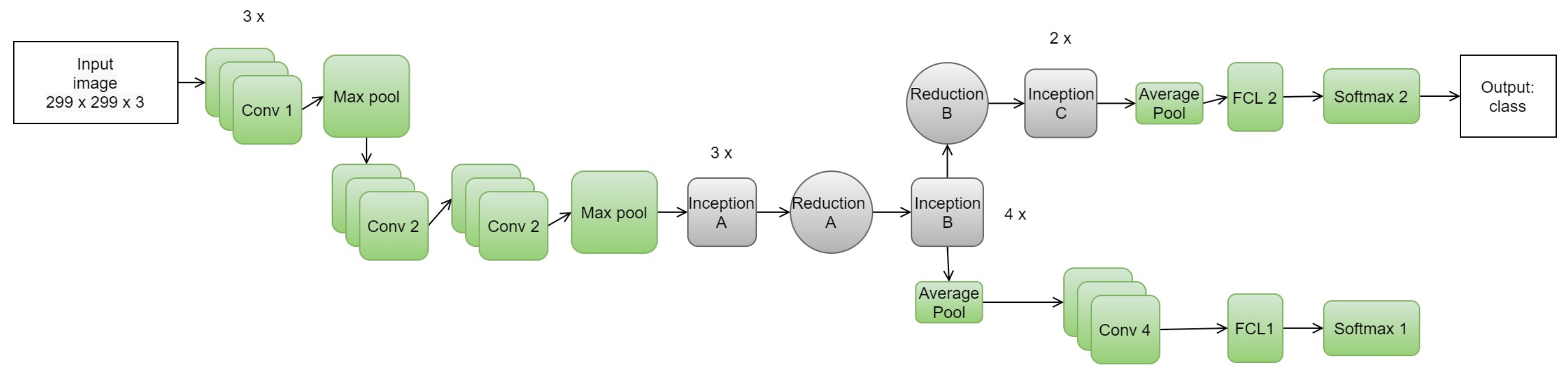
The Inception version 3 has 48 layers. Inception has an intermediate classifier. This classifier is a softmax layer that is used to help with varnish gradient problems by simply applying the loss in the second softmax function, in order to improve the results. Inception-v3 is shown in
Figure 11.
The authors evaluated inception-v3 [
52] on ILSVRC-2012 ImageNet validation set. The results were considered state-of-the-art, with a top-1 and top-5 error of 21.2% and 5.6% respectively.
5.4. ResNet
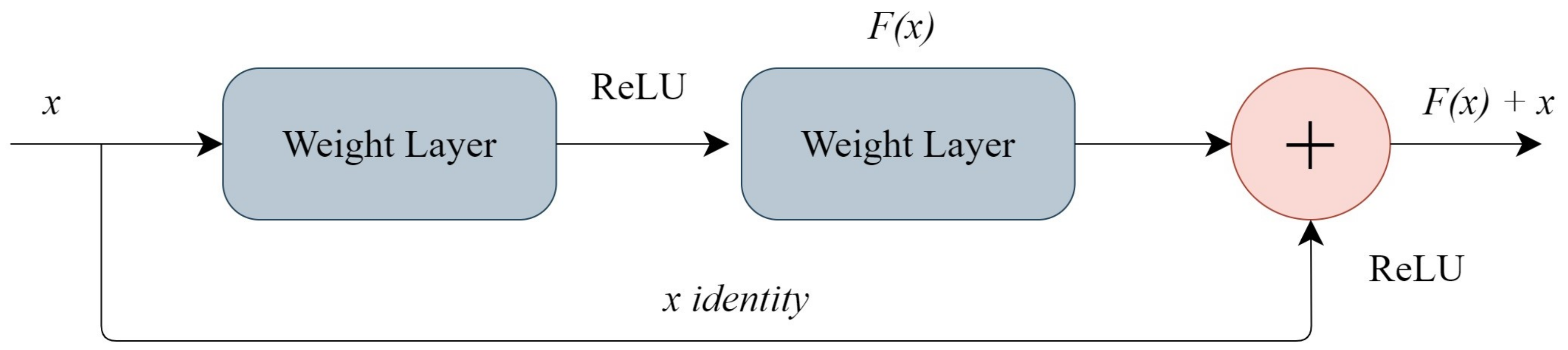
The Residual Networks (Resnets) are CNNs that learn residual functions referenced to inputs. Reference He et al. [
53] proposed a framework for deep networks that prevent saturation and degradation of the accuracy by shortcut connections that add identity map outputs to the output of skipped stacked layers. ResNets showed that the idea of stacking layers to improve results in complex problems has a limit, and the capacity of learning is not progressive. Reference He et al. [
53] introduced a residual block, enabling the creation of an identity map, bypassing the output from a previous layer into the next layer.
Figure 12 shows the residual block of Resnet.
The
x represents the input of a layer, and it is added together with the output
F(
x). Since
x and
F(
x) can have different dimensions due to convolutional operations, a certain W weight function is used to adjust the parameters, allowing the combination of
x and
F(
x) by changing the channels to match with the residual dimension. This operation is illustrated in Equations (
4) and (
5), where
x represents the input and
x + 1 is the output of an
i-th layer.
F represents the mentioned residual function. The identity map
h(
x) is equal to
xi and
f is a Rectified Linear Unit (ReLU) [
54] function implemented on the block, which provides better generalization and enhances the speed of convergence. Equation (
6) shows the ReLU function
Moreover, the Resnets use stochastic gradient descent (SGD) in the opposite of adaptative learning techniques [
55]. The authors introduced to the networks a pre-processing stage on the data, dividing the input in patches to introduce it to the network. This operation has the goal of improving the training performance of the network, which stacks residual blocks rather than layers. The activation of units is the combination of activation of the unit with a residual function. This tends to propagate the gradients through shallow units, improving the efficiency of training in Resnets [
56].
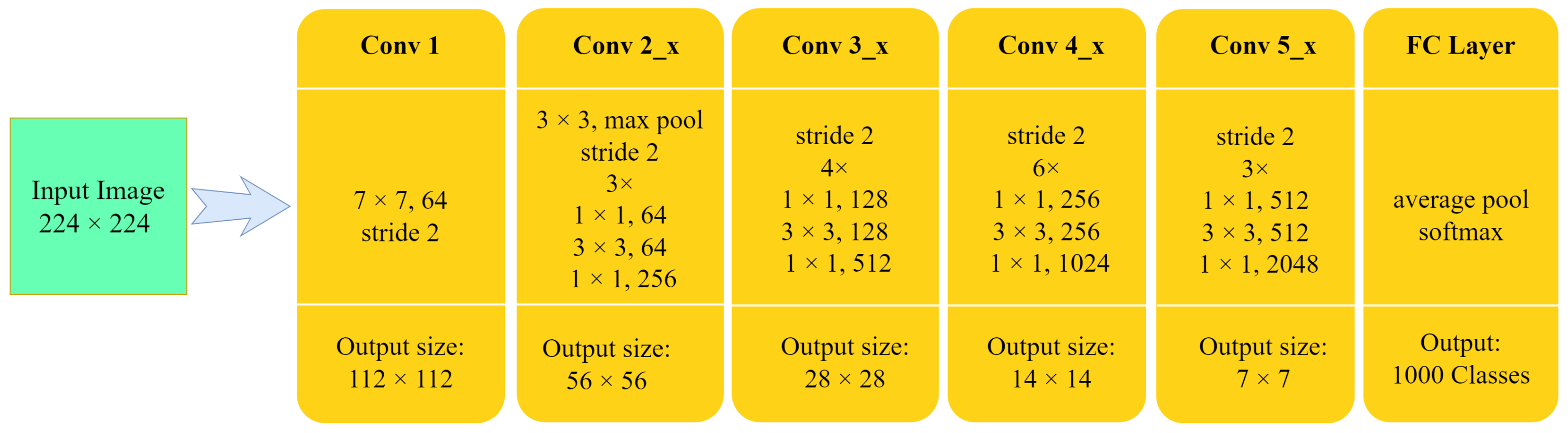
One of the versions of Resnets, Resnet50 was originally trained on the ImageNet 2012 dataset for the classification task of 1000 different classes [
57]. In total, Resnet50 runs
operations.
Figure 13 illustrates the Resnet50 architecture.
5.5. SqueezeNet
In their architecture, Iandola et al. [
58] proposed a smaller CNN with 50 times fewer parameters than AlexNet, however, keeping the same accuracy, bringing faster training, making model updates easier to achieve, and a feasible FPGA and embedded deployment. This architecture is called SqueezeNet.
SqueezeNet uses three strategies to build its structure. The 3 × 3 filters are replaced by 1 × 1, in order to reduce the number of parameters. The input channel is also modified, limiting its number to 3 × 3 filters. SqueezeNet also uses a late downsample approach, creating larger activation maps. Iandola et al. [
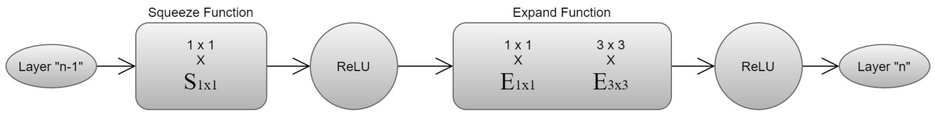
58] made use of fire modules, a squeeze convolution, and an expanded layer.
Figure 14 shows the fire module. It can be tuned in three locations: the number of 1 × 1 filters in the squeeze layer, represented by
. The number of 1 × 1 filters on expanding layer (
) and finally, the number of 3 × 3 filters also on expanding layer, represented by
. The first two hyperparameters are responsible for the implementation of strategy 1. The fire blocks also implement strategy 2, limiting the number of input channels by following a rule:
has to be less than
+
.
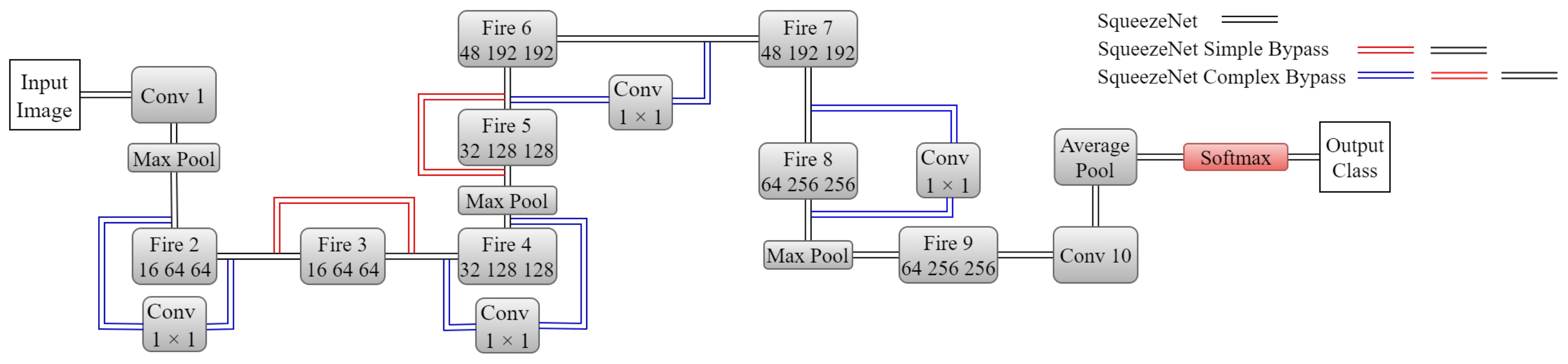
SqueezeNet has three different architectures, resumed in
Figure 15: SqueezeNet, SqueezeNet with skip connections, and SqueezeNet with complex skip connections, using 1 × 1 filters on the bypass. The fire modules are represented by the “fire” blocks, and the three numbers on them are the hyperparameters s1 × 1, e1 × 1, and e3 × 3 respectively. SqueezeNets are fully convolutional networks. The late downsample from strategy three is implemented by a max pooling, creating larger activation maps.
These bypasses are implemented to improve the accuracy and help train the model and alleviate the representational bottleneck. The authors trained the regular SqueezeNet on ImageNet ILSVRC-2012, achieving 60.4% top-1 and 82.5% top-5 accuracy with 4.8 megabytes as model size.
5.6. DenseNet
A CNN architecture that connects every layer to all layers was proposed by Huang et al. [
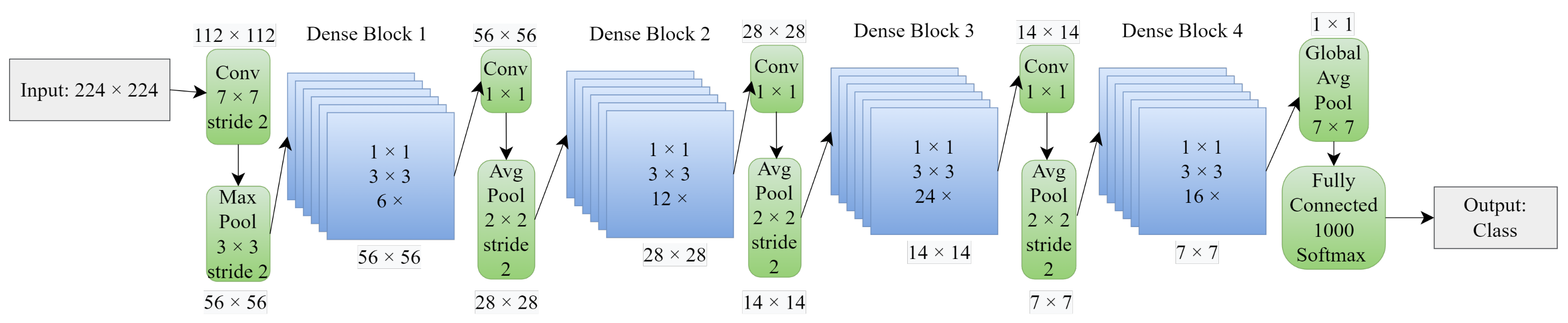
59]. This architecture called DenseNet works with dense blocks. These blocks connect each of the feature maps from preceding layers to all subsequent layers. This approach reuse features from the feature maps, compacting the model in an implicit deep supervision way.
DenseNet has four variants, each one with a different number of feature maps in their four “dense blocks”. The first variant, DenseNet-121 has the smallest depth on its blocks. It is represented in
Figure 16. Transition layers are in between the dense blocks and are composed of convolution and max pool operations. The architecture ends with a softmax to perform the final classification. As the depth increases, accuracy also increases, reporting no sign of degradation or overfitting [
59].
5.7. EfficientNet
EfficientNets [
60] are architectures that have a compound scaling, balancing depth, width, and resolution to achieve better performance. The authors proposed a family of models that follow a new compound scale method, using a coefficient
to scale their three dimensions. For depth:
d =
. Width:
w =
. Finally, resolution:
r =
. So that,
and
,
,
1. The
,
, and
are constants set by a grid search. The coefficient
indicates how many computational resources are available.
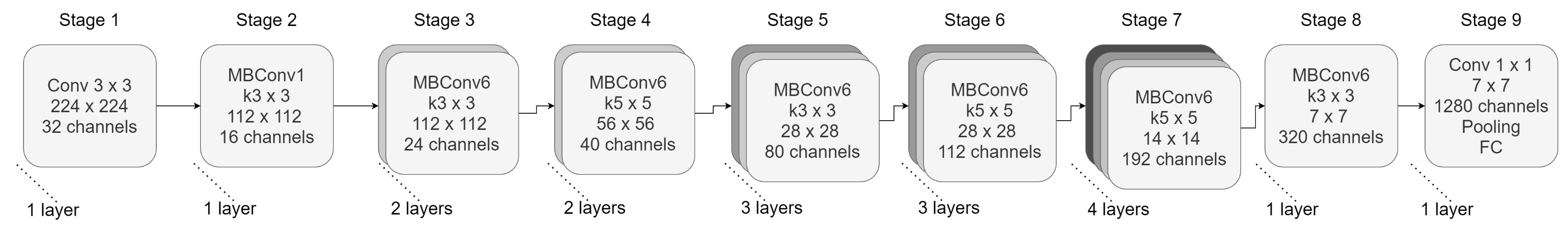
The models are generated by a multi-objective neural architecture search, optimizing accuracy and Floating-point operations per second, or FLOPS. They have a baseline structure inspired by residual networks and a mobile inverted bottleneck MBConv. The base model is presented in
Figure 17, known as EfficientNet-B0.
As more computational units are available, the blocks can be scaled up, from EfficientNet-B1 to B7. The approach searches for these three values on a small baseline network, avoiding spending that amount of computation [
60]. EfficientNet-B7 has 84,3% top-1 accuracy on ImageNet, a state-of-the-art result.
6. Ensemble Learning Approaches
Ensemble learning has gained attention on artificial intelligence, machine learning, and neural network. It builds classifiers and combines their output to reduce variances. By mixing the classifiers, ensemble learning improves the accuracy of the task, in comparison to only one classifier [
61]. Improving predictive uncertainty evaluation is a difficult task and an ensemble of models can help in this challenge [
62]. There are several ensembles approaches, suitable for specific tasks: Dynamic Selection, Sampling Methods, Cost-Sensitive Scheme, Patch-Ensemble Classification, Bagging, Boosting, Adaboost, Random Forest, Random Subspace, Gradient Boosting Machine, Rotation Forest, Deep Neural Decision Forests, Bounding Box Voting, Voting Methods, Mixture of Experts, and Basic Ensemble [
61,
63,
64,
65,
66,
67,
68].
For deep learning applications, an ensemble classification model generates results from “weak classifiers” and integrates them into a function to achieve the final result [
65,
66]. This fusion can be processed in ways like hard voting, choosing the class that was most voted or a soft voted, averaging or weighing an average of probabilities [
68]. Equation (
7) illustrates the soft voting ensemble method. The vector
represents the probabilities of classes in an n-classifier. The value of
is the weight of the n-classifier, in the range from 0 to 1. The final classification is the sum of all vectors of probabilities used on the ensemble, multiplied with their respective weights. The sum of weights must follow the rule described in Equation (
8)
The ensemble is a topic of discussion and it has been applied with deep learning and computer vision in tasks like insulator fault detection method using aerial images [
67], to recognize transmission equipment on images taken by an unmanned aerial vehicle [
68], and application of remote sensing image classification [
69]. There are also studies that compare imbalanced ensemble classifiers [
63].
9. Discussion and Conclusions
To create the synthetic dataset, Blender was used with Eevee as the render engine due to speed. Eevee was almost seven times faster than Cycles engine.
For the real dataset, the mechanical device performed the data gathering. It was built prior to the automated stacker being constructed. This enabled to testing of the CNNs with the real dataset. The Brisque IQA algorithm and the histogram analysis provided quality control for the real images.
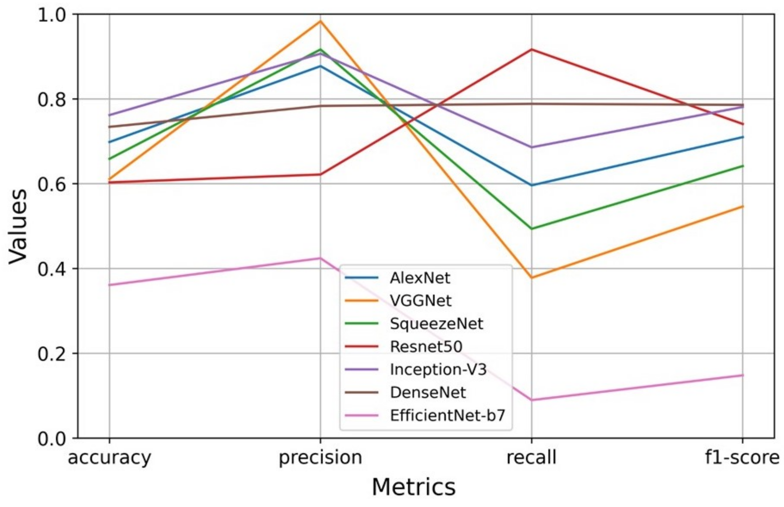
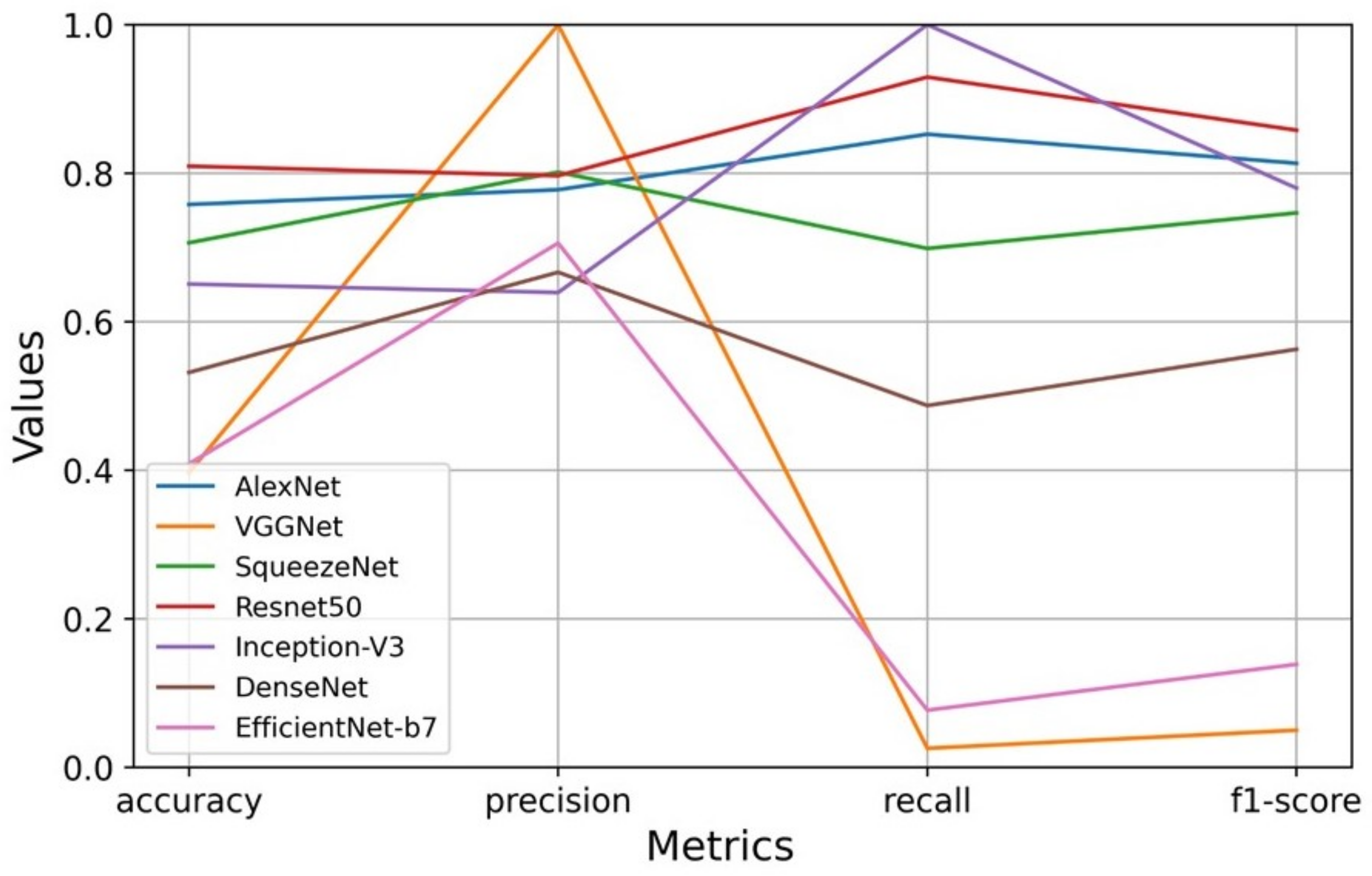
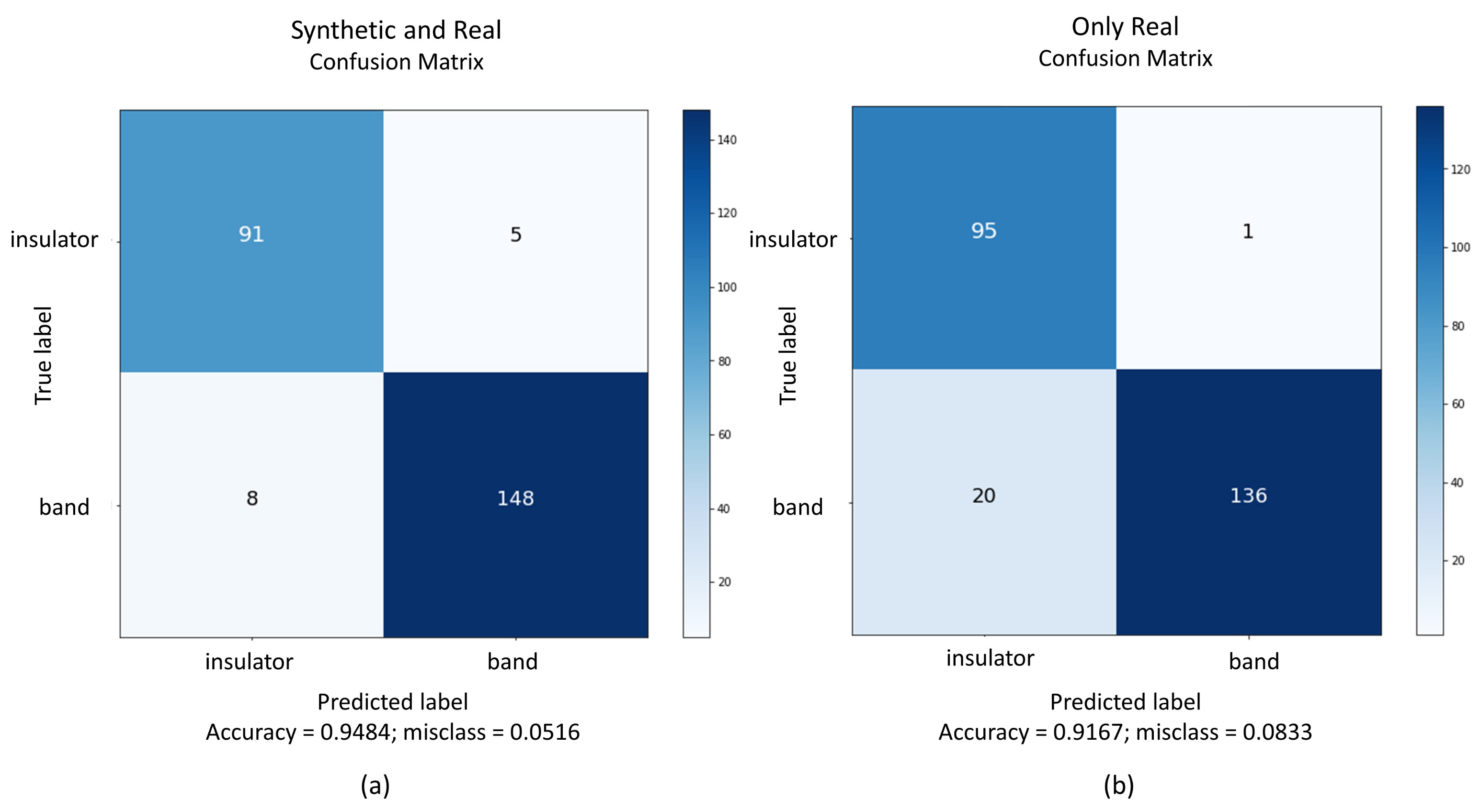
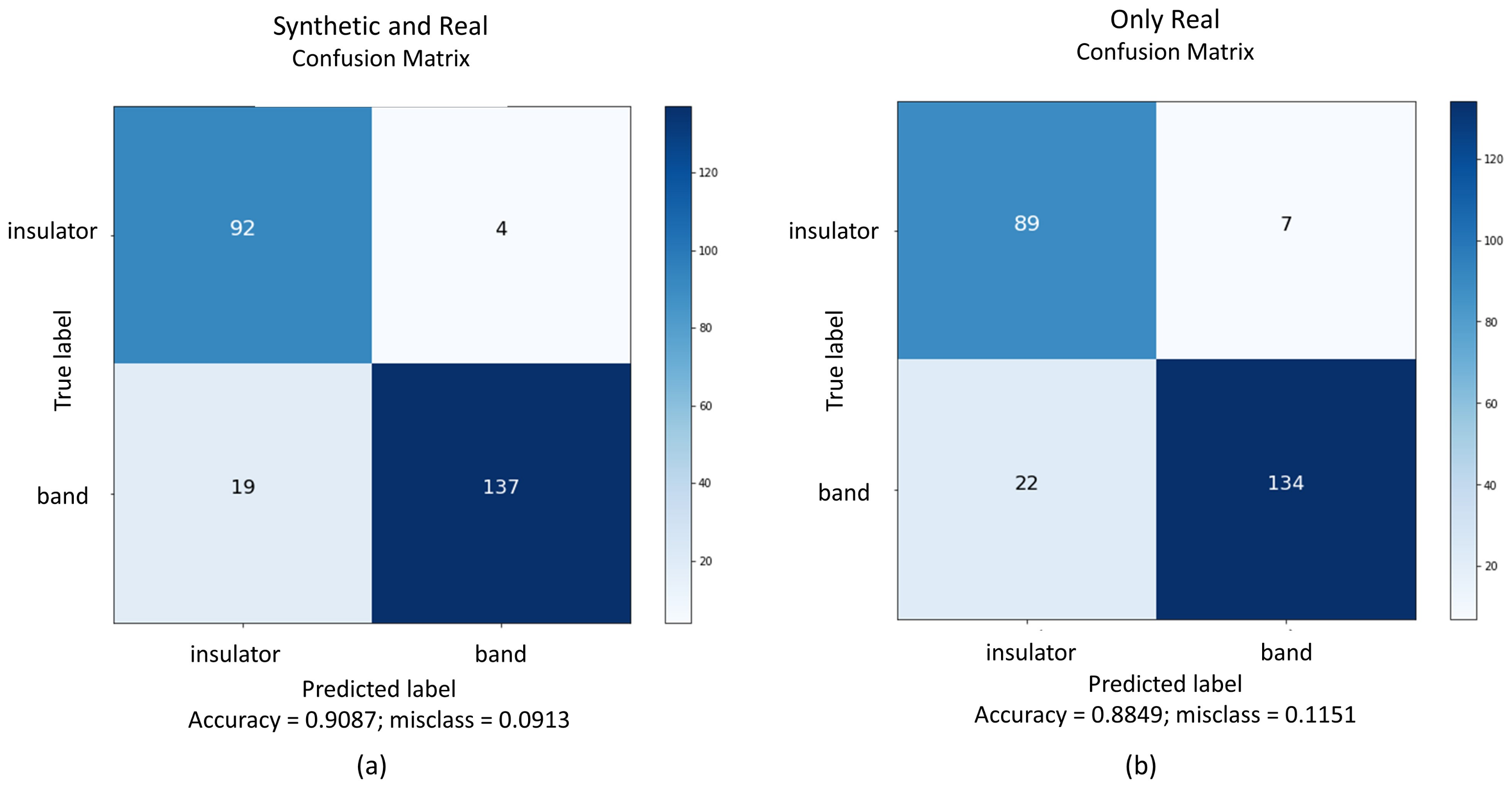
From the seven CNNs fine-tuned on the synthetic dataset and tested on the real domain, the best performance in RGB and RGB-D was respectively DenseNet and Resnet-50. The training procedure on synthetic datasets and testing on real samples showed a domain shift problem, a common issue discussed in recent studies. To contour this problem, a set of real images was separated and used to fine-tune DenseNet and Resnet. Fine-tuning the models with synthetic and then with real images outperformed classification in comparison with a straight fine-tuning on real images. The use of synthetic images generated by Blender and rendered by Eevee proved to help the classification performance.
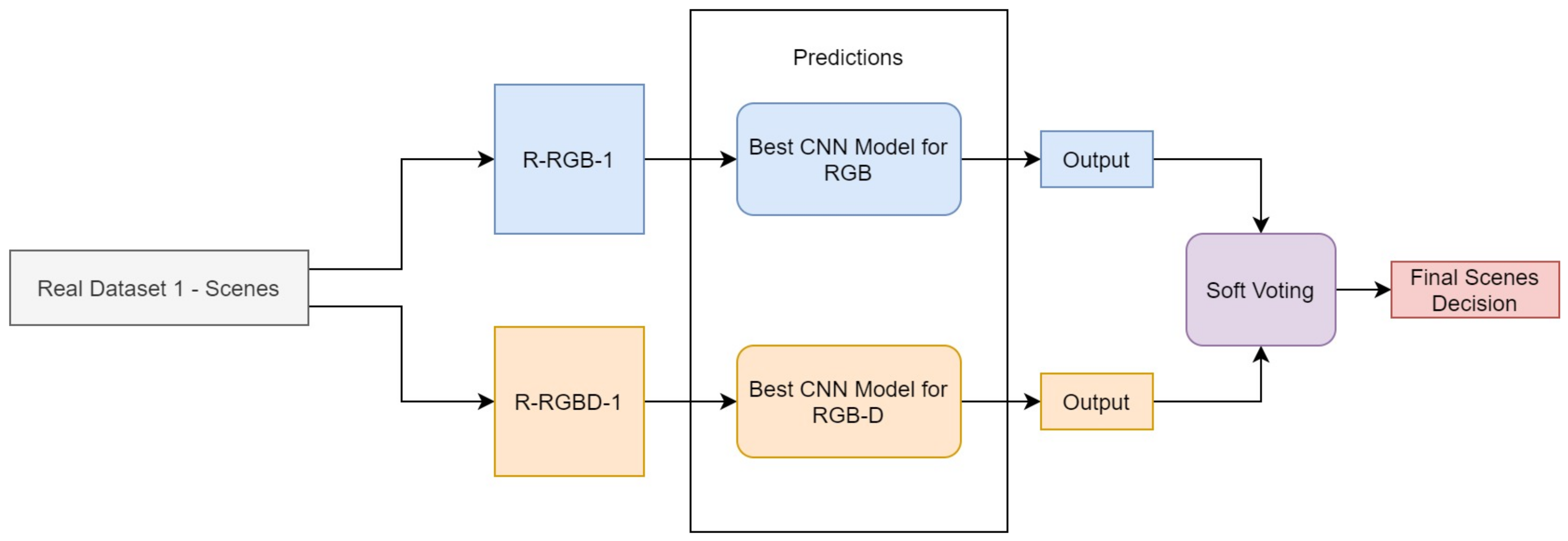
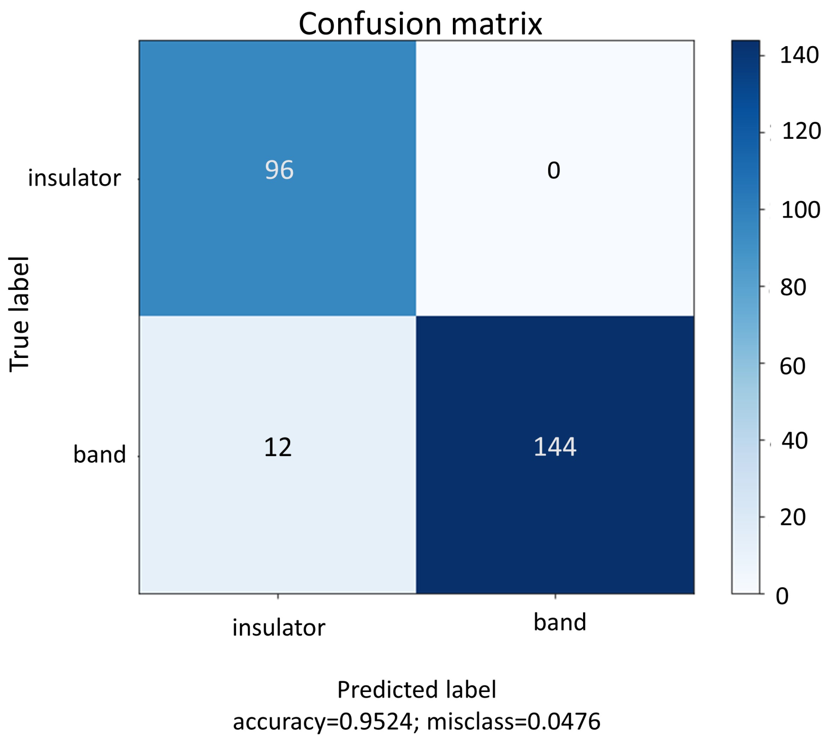
The proposed blended RGB and RGB-D pipelines were used to improve the recognition of insulators and brace bands. Since the scenes have colored and depth information, they were applied in an ensemble approach. Each pipeline contributed equally to the output prediction of the scenes, in a soft voting decision. The final classification is the average of probabilities of colored and depth pipelines. The blended approach outperformed the best results of the single CNNs, with the only exception being the metric recall in the DenseNet colored test. However, the blended pipelines misclassed fewer items in comparison with DenseNet. Blending colored and depth CNN pipelines achieved better accuracy in comparison with the previous study, where a Resnet-50 was used to classify the insulators and brace bands through RGB images [
2]. This present approach resulted in an accuracy of 95.23% in contrast to 92.87% seen in Piratelo et al. [
2].
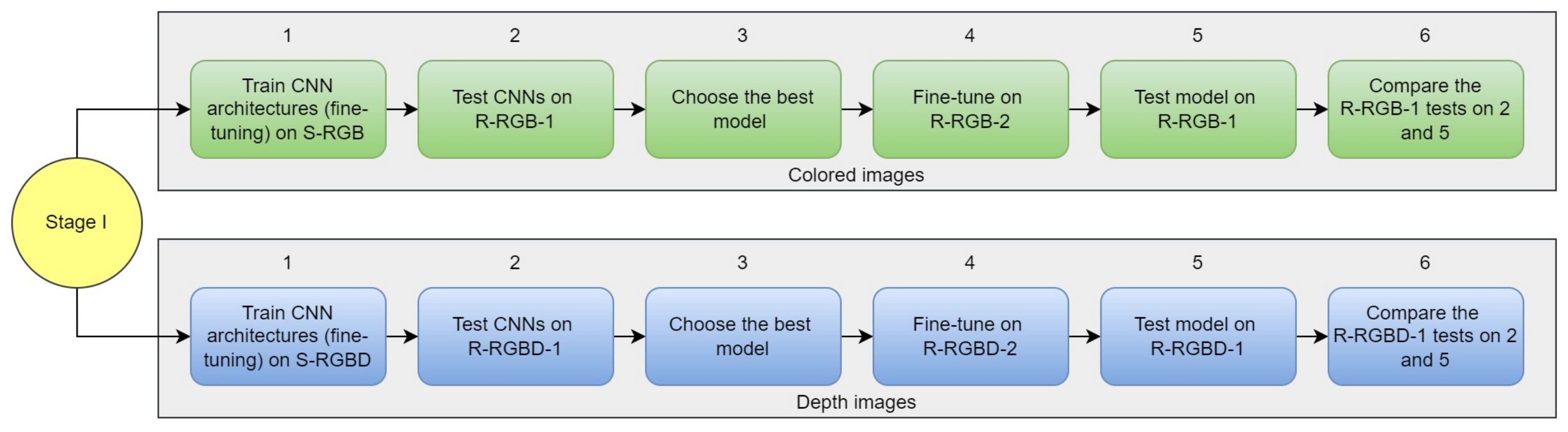
This paper presented a blend of convolutional neural network pipelines that classifies products from an electrical company’s warehouse, using colored and depth images from real and synthetic domains. The research also compared the results of training the architectures only with real and then synthetic and real data. The stage I consisted in training several CNNs on a synthetic dataset and testing them in the real domain. The architectures that performed better in RGB and RGB-D images were DenseNet and Resnet-50, although, they all suffered from the domain shift. A procedure to overcome this issue was done by fine-tuning the CNNs on a real set of data. The procedure improved the accuracy, precision, recall, and f1-score of the models in comparison to only training with real data, proving that synthetic images helped to train the models. It was time-consuming and it required a computational effort to train all CNNs on synthetic and real images, yet it showed to be a valid method to improve accuracy.
On stage II, the DenseNet model trained on RGB images was used as the first pipeline, and Resnet trained on RGB-D images composed the ensemble as the second pipeline. Each one contributed equally to the final classification, using the average of their probabilities in a soft voting method. A poorly performance of one CNN could drag down final accuracy for the ensemble. Both pipelines must be tuned with suitable accuracy. Moreover, this requires more computational resources in comparison with inferences from single CNNs on Stage I, since it is working with two models. However, the ensemble lead to a more robust classification, taking advantage of colored and depth information provided by the images, extracting features from both domains. The blended pipelines outperformed accuracy, precision, and f1-score in comparison with the single CNNs.
This approach intends to be encapsulated and used to keep the inventory of the warehouse up to date. The classification task is handled by computer vision and artificial intelligence, making full use of RGB and RGB-D images of synthetic and real domains, applied in an approach of blended CNN pipelines. The quality of captured images is also examined by an IQA called BRISQUE, equalizing the images and enhancing their features.
This study classifies two types of objects: insulators and brace bands. A transfer learning method called fine-tuning took advantage of pre-trained models, utilizing its feature detection capacity and adapting it to the problem. This transfer learning technique was used twice, first with synthetic and then with real images. The extensive tests conducted on this paper evaluated the performance of different CNNs individually and blended in an ensemble approach. In the end, the blend was able to classify the objects with an average accuracy of 95.23%. The tool will be included in the prototype of an AGV that travels the entire warehouse capturing images of the shelves, combining the application of automation, deep learning, and computer vision in a real engineering problem. This is the first step to automate and digitize the warehouse, seeking to achieve the paradigms of real-time data analysis, smart sensing, and perception of the company.
As future work, it is intended to test weights for the pipelines and seek their best combination. It is compelling to find different alternatives to ensemble learning techniques. A study of the combination between synthetic and real domain and their influence on training the models is also intended to be accomplished.


 and
and 


