Stability Anomalies of Some Jacobian-Free Iterative Methods of High Order of Convergence

Abstract

In this manuscript, we design two classes of parametric iterative schemes to solve nonlinear problems that do not need to evaluate Jacobian matrices and need to solve three linear systems per iteration with the same divided difference operator as the coefficient matrix. The stability performance of the classes is analyzed on a quadratic polynomial system, and it is shown that for many values of the parameter, only convergence to the roots of the problem exists. Finally, we check the performance of these methods on some test problems to confirm the theoretical results.

1. Introduction

Systems of nonlinear equations must usually be solved when nonlinear models, appearing in Science and Engineering, are discretized. There are no analytical techniques for solving these systems, so we approach their solutions by using iterative schemes. Although the most known iterative procedure is Newton’s scheme, in recent years, the focus of this area of research has been in constructing new iterative methods, trying to improve Newton’s one, in terms of convergence, efficiency, and stability (see, for example, some third-order schemes in References [1,2,3,4,5,6], or higher-order ones in References [7,8,9,10,11,12]). The key fact to get the most efficient methods is to evaluate as few Jacobian matrices as possible, per iteration (see Reference [13] and the references therein).

In 2016, the authors of [14] proposed a parametric class of iterative schemes with fourth-order of convergence, including a very efficient fifth-order procedure. The efficiency index used is defined as $p^{1/d+op}$, where p is the order of convergence of the method, d the number of functional evaluations per iteration, and $op$ the number of products/quotients used for obtaining a new iterate. This class combined three evaluations of the nonlinear function and only one of the Jacobian matrix, per iteration. In addition to the study of the local convergence and the computational cost of an iterative method, we must analyze its dependence on the set of initial estimations used. This analysis was made in Reference [15].

In this manuscript, we modified this class of iterative methods to avoid the calculation of Jacobian matrices, getting two different families, whose difference is based on the order of the estimation of the Jacobian matrix. Then, using the real multidimensional dynamics, we studied the behavior of the elements of the family (usually with the same order of convergence) and decided which ones are the best, from this point of view. Specifically, we studied the multipliers of the strange fixed points, analyzed the asymptotical behavior of the free critical points, and found different kinds of strange attractors using bifurcation diagrams. At the end, the dynamical planes are shown to check the theoretical results.

Introductory Concepts

Now, let us recall some concepts that we will use along this manuscript. Let $F(x)=0$ be a system of n equations with n variables, where $F:D\subseteq {\mathbb{R}}^n\to {\mathbb{R}}^n$, with coordinate functions $f_i$, $i=1,2,\dots ,n$. Our aim is to find a solution $\overline{x}\in D$ as a fixed point of the iteration method:

$$x^{(k+1)}=\overline{G}(x^{(k)}),k=0,1,\dots ,$$

(1)

$x^{(0)}$ being the initial guess.

Let us denote with $G(x)$ the vectorial fixed-point rational function associated to the iterative method applied to n-variable polynomial system $p(x)=0$, $p:{\mathbb{R}}^n\to {\mathbb{R}}^n$, $x\in {\mathbb{R}}^n$ $p(x)$. Most of the following concepts are direct extensions of those considered in complex dynamics (see, for example, [16,17]). The orbit of $x^{(0)}\in {\mathbb{R}}^n$ is defined as $\left\{x^{(0)},G(x^{(0)}),\dots ,G^m(x^{(0)}),\dots \right\}$. A point $x^{*}\in {\mathbb{R}}^n$ is a fixed point of G if $G(x^{*})=x^{*}$, and its stability is characterized in a result from Robinson ([16], p. 558), stating that the character of a period-k point $x^{*}$ depends on the eigenvalues of $G^{\prime }(x^{*})$, ${\lambda }_1,{\lambda }_1,\dots ,{\lambda }_n$. It is attracting if all $|{\lambda }_j|<1$, repelling if all $|{\lambda }_j|>1$ ($j=1,2,\dots ,n$)), and unstable or saddle if at least one ${\lambda }_{j_0}$ exists such that $|{\lambda }_{j_0}|>1$. In addition, a fixed point is called hyperbolic if all the eigenvalues ${\lambda }_j$ of $G^{\prime }(x^{*})$ have $|{\lambda }_j|\ne 1$.

On the other hand, if an iterative scheme has at least order two, then the zeroes of the function are superattracting fixed points of G. We call a strange fixed point to that not being a zero of $p(x)$. The basin of attraction $\mathcal{A}(x^{*})$ of an attracting fixed point $x^{*}$ of G, is $\mathcal{A}(x^{*})=\left\{x^{(0)}\in {\mathbb{R}}^n:G^m(x^{(0)})\to x^{*},m\to \infty \right\}$.

A point $x\in {\mathbb{R}}^n$ is a critical point of G if the eigenvalues of $G^{\prime }(x)$ are null. Therefore, if $g_i$ satisfies $\frac{\partial g_i(x)}{\partial x_j}=0$ for all $i,j\in \{1,\dots ,n\}$, then x is a critical point. If it is not a root of polynomial $p(x)$, it is called a free critical point.

In this manuscript, we apply these techniques (as it has been previously made, for example, in Reference [17]), to a couple of Jacobian-free families of iterative schemes. Specifically, we study the strange fixed points and their stability, prove the existence of free critical points, and find different chaotic behaviors (strange attractors, period-doubling cascades, etc.). In the last section, some basins of attraction are shown to visualize the performance of the elements of the family. Some numerical results are presented.

2. Jacobian-Free Parametric Families

We propose the following Jacobian-free version of a fourth-order iterative class designed by the authors of [14], denoted by M41, whose iterative expression is:

$$\begin{array}{ccc}\hfill y^{(k)}& =& x^{(k)}-H{(x^{(k)})}^{-1}F(x^{(k)}),k\ge 0\hfill \\ \hfill z^{(k)}& =& y^{(k)}-\beta H{(x^{(k)})}^{-1}F(y^{(k)}),\hfill \\ \hfill x^{(k+1)}& =& z^{(k)}+\frac{1}{\beta }H{(x^{(k)})}^{-1}\left({(\beta -1)}^{2}F(y^{(k)})-F(z^{(k)})\right),\hfill \end{array}$$

(2)

being $H(x^{(k)})=\left[x^{(k)},x^{(k)}+F(x^{(k)});F\right]$.

Because of the technique used in the proof, these methods have an order of convergence four in a neighborhood of $\overline{x}$, where $F^{\prime }(\overline{x})$ is nonsingular. The following result shows its local convergence, using the notation about the Taylor expansion of $F(x^{(k)})$ and $F^{\prime }(x^{(k)})$ around $\overline{x}$, introduced in Reference [18]. To get the Taylor expansion of the divided difference operator $[·,·;F]:D\times D\subset {\mathbb{R}}^n\times {\mathbb{R}}^n\to \mathcal{L}({\mathbb{R}}^n)$ (see Ortega-Rheimboldt [19]), its integral expression is used (known as the Genochi–Hermite formula):

$$[x+h,x;F]={\int }_0^1{F}^{\prime }(x+th)dt=F^{\prime }(x)+\frac{1}{2}{F}^{″}(x)h+\frac{1}{6}{F}^{‴}(x)h^2+O(h^3).$$

Theorem 1.

Let $\overline{x}\in D$ be a zero of $F:D\subset {\mathbb{R}}^n\to {\mathbb{R}}^n$, a sufficiently differentiable Frechét function in an open convex set D. Let us assume that $F^{\prime }(\overline{x})$ is nonsingular and let $x^{(0)}$ be an initial estimation near to $\overline{x}$. Class (2) has fourth-order of convergence for any $\beta \in \mathbb{R}$, $\beta \ne 0$. The error equation of the family is:

$$\begin{array}{ccc}\hfill e_{k+1}& =& \left[(5-\beta )C_2^2+2(3-\beta )C_2^3{F}^{\prime }(\overline{x})+3C_2^2{F}^{\prime }(\overline{x})C_2(I+F^{\prime }(\overline{x}))\right.\hfill \\ & & \left.+2C_2{F}^{\prime }(\overline{x})C_2^2(I+F^{\prime }(\overline{x}))-(\beta -1)C_2^3{F}^{\prime }{(\overline{x})}^2\right]e_k^4+O(e_k^5),\hfill \end{array}$$

being $C_k=(1/k!){\left[F^{\prime }(\overline{x})\right]}^{-1}{F}^{(k)}(\overline{x})$, $k=2,3,\dots$, $e_k=x^{(k)}-\overline{x}$, $k\ge 0$, and I denotes the $n\times n$ identity matrix.

Proof. 

The Taylor development of $F(x^{(k)})$ around $\overline{x}$ is:

$$F(x^{(k)})=F^{\prime }(\overline{x})\left[e_k+C_2{e}_k^2+C_3{e}_k^3+C_4{e}_k^4\right]+O(e_k^5),$$

being also the expansion of its successive derivatives:

$$\begin{array}{ccc}\hfill F^{\prime }(x^{(k)})& =& F^{\prime }(\overline{x})\left[I+2C_2{e}_k+3C_3{e}_k^2+4C_4{e}_k^3\right]+O(e_k^4),\hfill \\ \hfill F^{″}(x^{(k)})& =& F^{\prime }(\overline{x})\left[2C_2+6C_3{e}_k+12C_4{e}_k^2\right]+O(e_k^3),\hfill \\ \hfill F^{‴}(x^{(k)})& =& F^{\prime }(\overline{x})\left[6C_3+24C_4{e}_k\right]+O(e_k^2).\hfill \end{array}$$

Then, denoting by $w^{(k)}=x^{(k)}+F(x^{(k)})$ and $e_w=w^{(k)}-\overline{x}$:

$$[x^{(k)},w^{(k)};F]=F^{\prime }(\overline{x})\left[I+C_2(e_k+e_w)\right]+O(h^3).$$

By forcing that ${[x^{(k)},w^{(k)};F]}^{-1}[x^{(k)},w^{(k)};F]=[x^{(k)},w^{(k)};F]{[x^{(k)},w^{(k)};F]}^{-1}=I$, it is obtained that:

$${[x^{(k)},w^{(k)};F]}^{-1}=\left[I-C_2(2+F^{\prime }(\overline{x}))e_k\right]{\left[F^{\prime }(\overline{x})\right]}^{-1}+O(h^2).$$

Then, the expansion of error at the first step of the iterative process $e_y=y^{(k)}-\overline{x}$ is:

$$e_y=e_k-{[x^{(k)},w^{(k)};F]}^{-1}F(x^{(k)})=C_2(I+F^{\prime }(\overline{x}))e_k^2+O(e_k^3),$$

and, therefore:

$$F(y^{(k)})=F^{\prime }(\overline{x})\left[e_y+C_2{e}_y^2\right]+O(e_y^3).$$

In a similar way, the Taylor expansion of the error at the second step $e_z=z^{(k)}-\overline{x}$ is:

$$e_z=e_y-\beta {[x^{(k)},w^{(k)};F]}^{-1}F(y^{(k)})=(1-\beta )e_y+\beta C_2(2I+F^{\prime }(\overline{x}))e_k{e}_y-\beta C_2{e}_y^2+O(e_k^5).$$

Then:

$$F(z^{(k)})=F^{\prime }(\overline{x})\left[e_z+C_2{e}_z^2\right]+O(e_z^3),$$

and:

$$\begin{array}{ccc}\hfill {[x^{(k)},w^{(k)};F]}^{-1}\left({(\beta -1)}^{2}F(y^{(k)})-F(z^{(k)})\right)& =& \left[I-C_2(2+F^{\prime }(\overline{x}))e_k\right]\hfill \\ & & \left[{(\beta -1)}^2{e}_y+{(\beta -1)}^2{C}_2{e}_y^2-e_z-C_2{e}_z^2\right]+O(e_k^5)\hfill \\ & =& \left[{(\beta -1)}^2{e}_y+{(\beta -1)}^2{C}_2{e}_y^2-e_z-C_2{e}_z^2\right.\hfill \\ & & \left.-{(\beta -1)}^2{C}_2(2+F^{\prime }(\overline{x}))e_k{e}_y+C_2(2+F^{\prime }(\overline{x}))e_k{e}_z\right]+O(e_k^5).\hfill \end{array}$$

Finally, the error equation of the method can be expressed as:

$$\begin{array}{ccc}\hfill e_{k+1}& =& e_z-\frac{1}{\beta }{[x^{(k)},w^{(k)};F]}^{-1}\left({(\beta -1)}^{2}F(y^{(k)})-F(z^{(k)})\right)\hfill \\ & =& \left[\frac{\beta -1}{\beta }{e}_z+\frac{{(\beta -1)}^2}{\beta }{e}_y-\frac{{(\beta -1)}^2}{\beta }{C}_2(2+F^{\prime }(\overline{x}))e_k{e}_y\right.\hfill \\ & & \left.+\frac{1-\beta }{\beta }{C}_2(2+F^{\prime }(\overline{x}))e_k{e}_y+C_2(2+F^{\prime }(\overline{x}))C_2(2+F^{\prime }(\overline{x}))e_k^2{e}_y\right]+O(e_k^5),\hfill \end{array}$$

that, expressed in terms of powers of $e_k$ and after some algebraic simplifications, results in:

$$\begin{array}{ccc}\hfill e_{k+1}& =& \left[(5-\beta )C_2^2+2(3-\beta )C_2^3{F}^{\prime }(\overline{x})+3C_2^2{F}^{\prime }(\overline{x})C_2(1+F^{\prime }(\overline{x}))\right.\hfill \\ & & \left.+2C_2{F}^{\prime }(\overline{x})C_2^2(1+F^{\prime }(\overline{x}))-(\beta -1)C_2^3{F}^{\prime }{(\overline{x})}^2\right]e_k^4+O(e_k^5),\hfill \end{array}$$

proving the fourth-order of convergence of all the elements of the family for any real $\beta \ne 0$. □

Now, if a second-order estimation of the Jacobian matrix is made in the original M4 family of Reference [14] in a similar way to that in Reference [20], then it can be expressed as:

$$\begin{array}{ccc}\hfill y^{(k)}& =& x^{(k)}-M{(x^{(k)})}^{-1}F(x^{(k)}),k\ge 0\hfill \\ \hfill z^{(k)}& =& y^{(k)}-\beta M{(x^{(k)})}^{-1}F(y^{(k)}),\hfill \\ \hfill x^{(k+1)}& =& z^{(k)}+\frac{1}{\beta }M{(x^{(k)})}^{-1}\left({(\beta -1)}^{2}F(y^{(k)})-F(z^{(k)})\right),\hfill \end{array}$$

(3)

where $M(x^{(k)})=\left[x^{(k)}+F(x^{(k)}),x^{(k)}-F(x^{(k)});F\right]$, which we denote as M42. The following result shows its local order of convergence.

Theorem 2.

Let $\overline{x}\in D$ be a zero of $F:D\subset {\mathbb{R}}^n\to {\mathbb{R}}^n$, a sufficiently differentiable Frechét function in an open convex set D. Let us assume that $F^{\prime }(\overline{x})$ is nonsingular, and let $x^{(0)}$ be an initial estimation near to $\overline{x}$. If $\beta \ne 0$, the family defined by (3) has, at least, fourth-order of convergence for any $\beta \in \mathbb{R}$, being fifth-order convergent when $\beta =5$. The error equation of the class is:

$$e_{k+1}=(5-\beta )C_2^3{e}_k^4+O(e_k^5),$$

being $C_k=(1/k!){\left[F^{\prime }(\overline{x})\right]}^{-1}{F}^{(k)}(\overline{x})$, $k=2,3,\dots$ and $e_k=x^{(k)}-\overline{x}$, $k\ge 0$.

Proof. 

By denoting $w^{(k)}=x^{(k)}+F(x^{(k)})$ and $s^{(k)}=x^{(k)}-F(x^{(k)})$ and in a similar way as in the proof of Theorem 1, the Taylor expression of the second-order divided difference and its inverse can be expressed as:

$$[w^{(k)},s^{(k)};F]=F^{\prime }(\overline{x})\left[I+2C_2{e}_k\right]+O(h^2),$$

and:

$${[x^{(k)},w^{(k)};F]}^{-1}=\left[I-2C_2{e}_k\right]{\left[F^{\prime }(\overline{x})\right]}^{-1}+O(h^2).$$

Then, the error at the first step is:

$$e_y=e_k-{[w^{(k)},s^{(k)};F]}^{-1}F(x^{(k)})=C_2{e}_k^2+O(e_k^3),$$

and again:

$$F(y^{(k)})=F^{\prime }(\overline{x})\left[e_y+C_2{e}_y^2\right]+O(e_y^3).$$

Thus, the expansion of the error at the second step is:

$$e_z=e_y-\beta {[w^{(k)},s^{(k)};F]}^{-1}F(y^{(k)})=(1-\beta )e_y+2\beta C_2{e}_k{e}_y-\beta C_2{e}_y^2+O(e_k^5).$$

Therefore:

$$\begin{array}{ccc}\hfill F(z^{(k)})& =& F^{\prime }(\overline{x})\left[e_z+C_2{e}_z^2\right]+O(e_z^3)\hfill \\ & =& F^{\prime }(\overline{x})\left[(1-\beta )e_y+2\beta C_2{e}_k{e}_y+(1+{\beta }^2-3\beta )e_y^2\right]+O(e_k^5),\hfill \end{array}$$

and:

$$\left({(\beta -1)}^{2}F(y^{(k)})-F(z^{(k)})\right)=F^{\prime }(\overline{x})\left[\beta (\beta -1)e_y-2\beta C_2{e}_k{e}_y+\beta C_2{e}_y^2\right]+O(e_k^5).$$

Finally, the error equation of the method can be expressed as:

$$\begin{array}{ccc}\hfill e_{k+1}& =& e_z-\frac{1}{\beta }{[w^{(k)},s^{(k)};F]}^{-1}\left({(\beta -1)}^{2}F(y^{(k)})-F(z^{(k)})\right)\hfill \\ & =& \left[I-2C_2{e}_k\right]\left[(\beta -1)e_y-2C_2{e}_k{e}_y+C_2{e}_y^2\right]+O(e_k^5),\hfill \end{array}$$

that, expressed in terms of $e_k$ and simplifying:

$$\begin{array}{ccc}\hfill e_{k+1}& =& \left(5-\beta \right)C_2^3{e}_k^4+O(e_k^5),\hfill \end{array}$$

proving that all the members of the class have, at least, fourth-order of convergence, except the element corresponding to $\beta =5$, which is fifth-order convergent. □

In the following sections, we use the properties of the discrete dynamical systems associated to these families in order to select their most stable members.

3. Multidimensional Dynamical Analysis

In the following, we denote by $M^i(x,\beta )=(M_1^i(x,\beta ),M_2^i(x,\beta ),\dots ,M_n^i(x,\beta ))$, $i=1,2$ the fixed point function associated to M41 and M42 classes, respectively, applied on n-dimensional quadratic polynomial $p(x)=0$, where:

$$\begin{array}{c}{p}_i(x)=x_i^2-1,i=1,2,\dots ,n.\hfill \end{array}$$

(4)

3.1. Class M41

As the polynomial system has separated variables, all the components of $M^i(x,\beta )$ (for a fixed $i\in \{1,2\}$) have the same expression, with the only difference of the sub-index corresponding to the component of x. In the case of method M41, the coordinate functions of the multidimensional rational operator can be expressed as:

$$\begin{array}{ccc}\hfill M_j^1(x,\beta )& =& x_j+\frac{1-x_j^2}{-1+2x_j+x_j^2}-\frac{x_j(2+x_j){\left(-1+x_j^2\right)}^2\beta }{{\left(-1+2x_j+x_j^2\right)}^3}\hfill \\ & & +\frac{1}{{\left(-1+2x_j+x_j^2\right)}^7}{x}_j(2+x_j){\left(-1+x_j^2\right)}^2\hfill \\ & & \left(x_j(6-10\beta )+x_j^3(14-4\beta )+x_j^8(-2+\beta )+6x_j^5(-1+\beta )+\beta \right.\hfill \\ & & \left.-6x_j^4(-7+4\beta )+2x_j^7(-7+4\beta )+x_j^6(-30+19\beta )+x_j^2(-26+19\beta )\right),\hfill \end{array}$$

for $j=1,2,\dots ,n$.

All the information about the stability analysis of these fixed points appears in the next result.

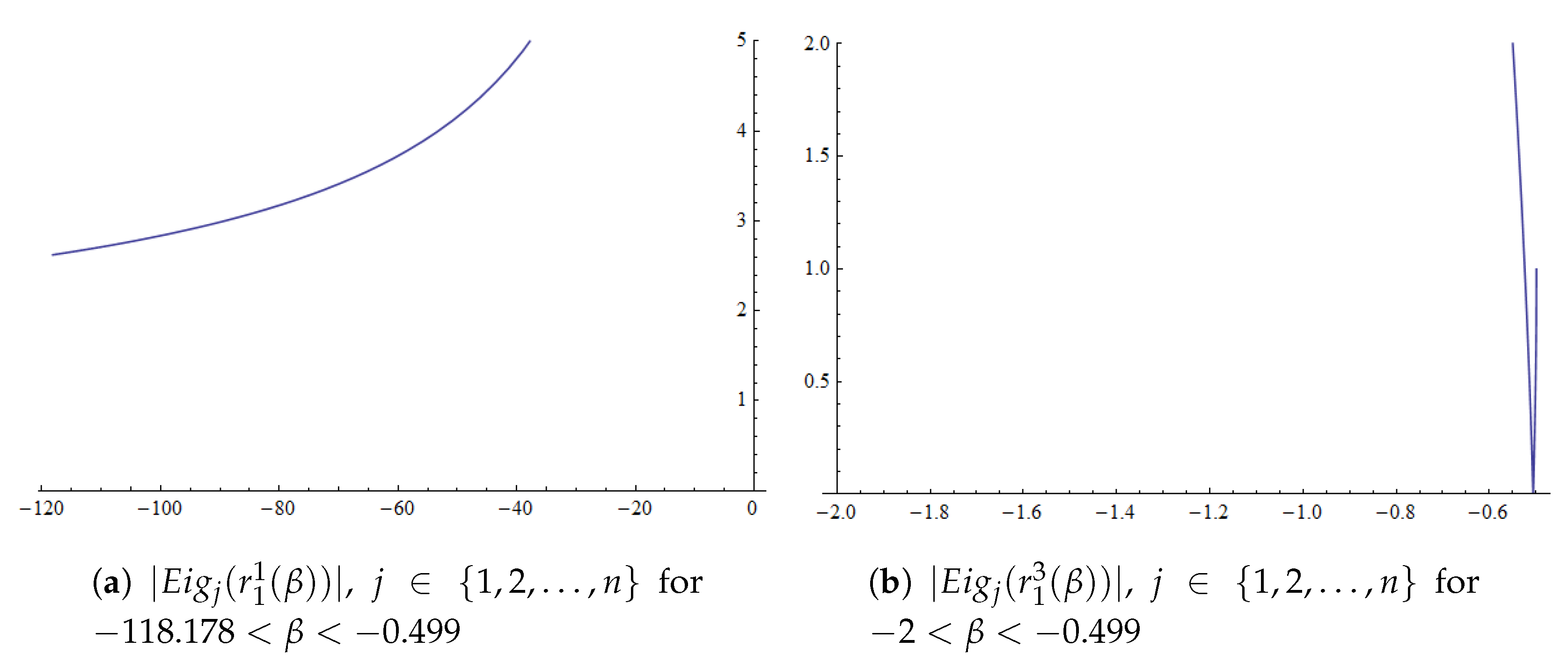
Theorem 3.

The $2^n$ roots of $p(x)$ are superattracting fixed points of the rational function associated to M41. This operator also has a different number of real strange fixed points whose values depend on β:

• If $\beta <-118.1782$, six roots of $r_1(t)$, denoted by $r_1^i(\beta )$, $i=1,2,\dots ,6$ are real, being their respective eigenvalues of the associate Jacobian matrix ${\lambda }_i(\beta )>1$, $i=1,2,\dots ,5$ and ${\lambda }_6(\beta )<1$.
• If $\beta =-118.1782$, five roots of $r_1(t)$, are real, being their respective eigenvalues of the associate Jacobian matrix ${\lambda }_i(-118.1782)>1$, $i=1,2,3,4$ and ${\lambda }_5(-118.1782)=1$.
• For $-118.1782<\beta <-0.4991$, there are four real roots of $r_1(t)$, being their respective eigenvalues of the associate Jacobian matrix ${\lambda }_i(\beta )>1$, $i=1,2,4$ and ${\lambda }_3(\beta )<1$ if $-0.5242<\beta <-0.4991$, ${\lambda }_3(\beta )>1$ for $118.1782<\beta <-0.5242$ and ${\lambda }_3(\beta )=1$ if $\beta =-0.5242$.
• If $\beta =-0.4991$, three roots of $r_1(t)$ are real, being their respective eigenvalues of the associate Jacobian matrix ${\lambda }_i(-0.4991)>1$, $i=1,2$ and ${\lambda }_3(-0.4991)=1$.
• For $-0.4991<\beta <0$ and $0<\beta <62.0613$, there are two real roots of $r_1(t)$ satisfying ${\lambda }_i(\beta )>1$, $i=1,2$.
• If $\beta =62.0613$, four roots of $r_1(t)$ are real, being their respective eigenvalues of the associate Jacobian matrix ${\lambda }_i(62.0613)=1$, $i=1,2$ and ${\lambda }_j(62.0613)>1$, $j=3,4$.
• When $\beta >62.0613$, there are four real roots of $r_1(t)$ satisfying ${\lambda }_i(\beta )>1$, $i=1,2,3,4$.

Proof. 

By solving the equation $M_j^1(x,\beta )=x_j$, the fixed points of the multidimensional rational function are obtained:

$$\frac{x_j^2-1}{{\left(-1+2x_j+x_j^2\right)}^7}{r}_1(x_j)=0,j=1,2,\dots ,n,$$

that is, they are $x_j=\pm 1$ and also the roots of the polynomial $r_1(t)=1-12t+(66-4\beta )t^2+(-146-4\beta )t^3+(5+11\beta )t^4+(312+12\beta )t^5+(-48-9\beta )t^6+(-332-12\beta )t^7+(-73+\beta )t^8+(148+4\beta )t^9+(110+\beta )t^{10}+30t^{11}+3t^{12}$, provided that $-1+2t+t^2\ne 0$.

However, as most six of the strange fixed points roots of $r_1(t)$ are real, depending on the value of $\beta$, let us denote them by $r_1^1(\beta )$ to $r_1^6(\beta )$. In order to analyze the stability of these fixed points, the eigenvalues of the associated Jacobian matrix:

$$Ei{g}_j(x_j(\beta ))=\frac{{\left(-1+x_j^2\right)}^3}{{\left(-1+2x_j+x_j^2\right)}^8}{s}_1(x_j),$$

being $s_1(t)=x_j^{10}+16x_j^9+95x_j^8+2(\beta +140)x_j^7+2(\beta +216)x_j^6+(288-14\beta )x_j^5-2(15\beta +28)x_j^4-4(11\beta +38)x_j^3-(52\beta +9)x_j^2-8(\beta -2)x_j+1$, are studied for $j=1,2,\dots ,n$. In each interval where the number of real strange fixed points changes, the Jacobian matrix is evaluated on them and the absolute value of their respective eigenvalues is analyzed. This procedure states the stability of the fixed points (see Figure 1a) for $r_1^1(\beta )$ as a component of the fixed point,$|Ei{g}_j(r_1^1(\beta ))|>1$, if $-118.178<\beta <-0.499$ and $|Ei{g}_j(r_1^3(\beta ))|<1$ for $-2<\beta <-0.499$.

Taking these results into account, those fixed points whose components are $\pm 1$ and/or $r_1^6(\beta )$ for $\beta <-118.1782$ are attracting. In a similar way, all the fixed points whose components are $\pm 1$ and $r_1^3(\beta )$ for $-0.5242<\beta <-0.4991$ are attracting. If a fixed point is composed exclusively by $r_1^6(\beta )$ and $r_1^3(\beta )$ out of these intervals of $\beta$, or by $r_1^1(\beta )$, $r_1^2(\beta )$, $r_1^4(\beta )$ and/or $r_1^5(\beta )$ for all values of $\beta$, it is repulsive. In any other case, the strange fixed point is classified as saddle. □

Now, we make a similar study for the second Jacobian-free class of iterative methods.

3.2. Family M42

When the rational operator associated to method M42 on $p(x)$ is analyzed, its coordinate functions can be expressed as:

$$\begin{array}{ccc}\hfill M_j^2(x,\beta )& =& -\frac{\beta +(\beta -40)x_j^8-4(\beta +30)x_j^6+(6\beta +40)x_j^4-4(\beta +2)x_j^2}{128x_j^7},\hfill \end{array}$$

for $j=1,2,\dots ,n$.

To calculate the fixed points of the multidimensional rational function, we get the roots of $M^2(x,\beta )=x$. We obtain again $x_j=\pm 1$ and also the real roots of the polynomial $r_2(t)=(\beta +88)t^6+(-3\beta -32)t^4+(3\beta +8)t^2-\beta$. It can be checked that $r_2(t)$ only has, at most, two real roots, which are denoted by $r_2^1(\beta )$ and $r_2^2(\beta )$. However, the rational function $M^2(x,\beta )$ is the same as that analyzed in Reference [15], corresponding to the original fourth-order iterative class designed by the authors of [14], who use Jacobian matrices in its iterative expression applied on $p(x)$.

Although the classes of iterative methods are different (that of Reference [14] uses Jacobian matrices and the proposed one is Jacobian-free), the second order estimation of the Jacobian matrix has the same effect on quadratic polynomial systems. So, the following result coincides with that of [14].

Theorem 4.

The $2^n$ roots of $p(x)$ are superattracting fixed points of the rational function associated to M42. This operator also has a different number of real strange fixed points whose values depend on β:

(a) 

If $\beta >0$ or $\beta <-88$, $r_2^1(\beta )$ and $r_2^2(\beta )$ are real, being their respective eigenvalues of the associate Jacobian matrix ${\lambda }_i(\beta )>1$, $i=1,2$.

(b) 

For $-88\le \beta \le 0$, the only real fixed points are the roots $z=\pm 1$ of $p(z)$; thus, there are no strange fixed points.

There also exist two free critical points with components $c_j(\beta )=\pm \sqrt{\frac{-7\beta }{\beta -40}}$, $j=1,2,\dots ,n$, for $\beta \in [0,40[$.

In the next section, we delve into the bifurcation analysis of these free critical points in order to locate other undesirable behaviors, such as attracting periodic orbits, strange attractors, etc.

4. Critical Points and Bifurcation Diagrams

Firstly, we analyze the case of class M41, that is, the rational function $M^1(x,\beta )$ and its critical points.

Theorem 5.

The components of the free critical points of operator $M^1(x,\beta )$ are the only ones making null all the partial derivatives of $M_j^1(x,\beta )$, for $j=1,2,\dots ,n$, that is, the solutions of $p(x)=0$ and also the real zeroes of the tenth-degree polynomial $s_1(t)$ depending on β, denoted by $c_i^1(\beta )$, $i=1,2,\dots ,8$:

(a) 

only four of them being real for $-910.178<\beta <-4.77238$;

(b) 

six for $\beta <-910.178$, $-4.77238<\beta <0.971327$, and $\beta >1$ and;

(c) 

there exist eight free different components of the critical points of $M(x)$ for $0.971327\le \beta <1$.

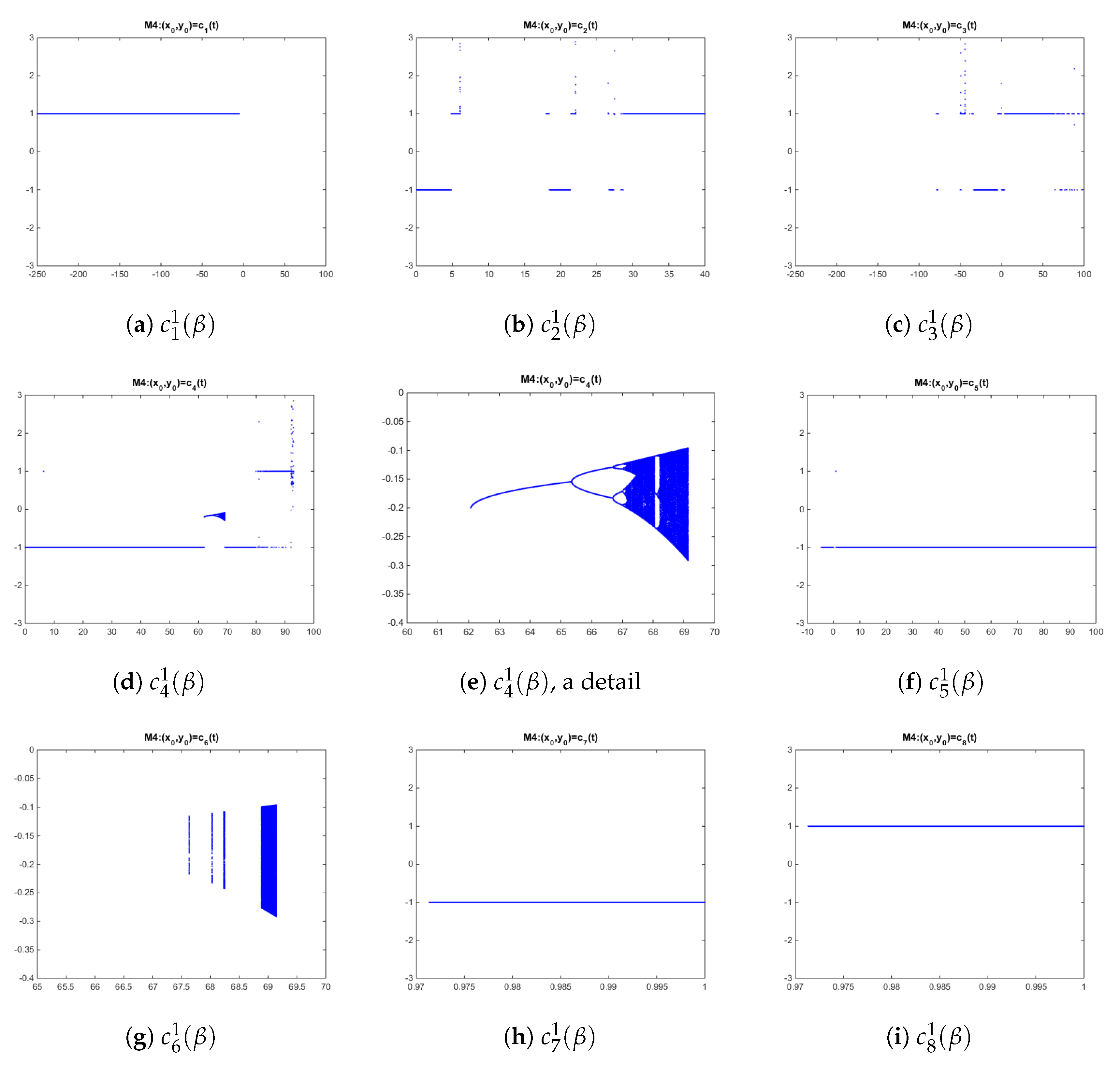
We use Feigenbaum diagrams to analyze the bifurcations of the map related to each family on system $p(x)$ using each one of the free critical points of the map as a starting point and observing their behavior for different ranges of $\beta$. When the rational function is iterated on these critical points, different behavior can be found after 1000 iterations of the method corresponding to each value of $\beta$ in a mesh of 3000 subintervals. The resulting behavior is from convergence to the roots to periodic orbits or even other attractors. In the case of class M41, we observe in Figure 2 the orbits of these critical points, in the range of $\beta$ where each one of them is real.

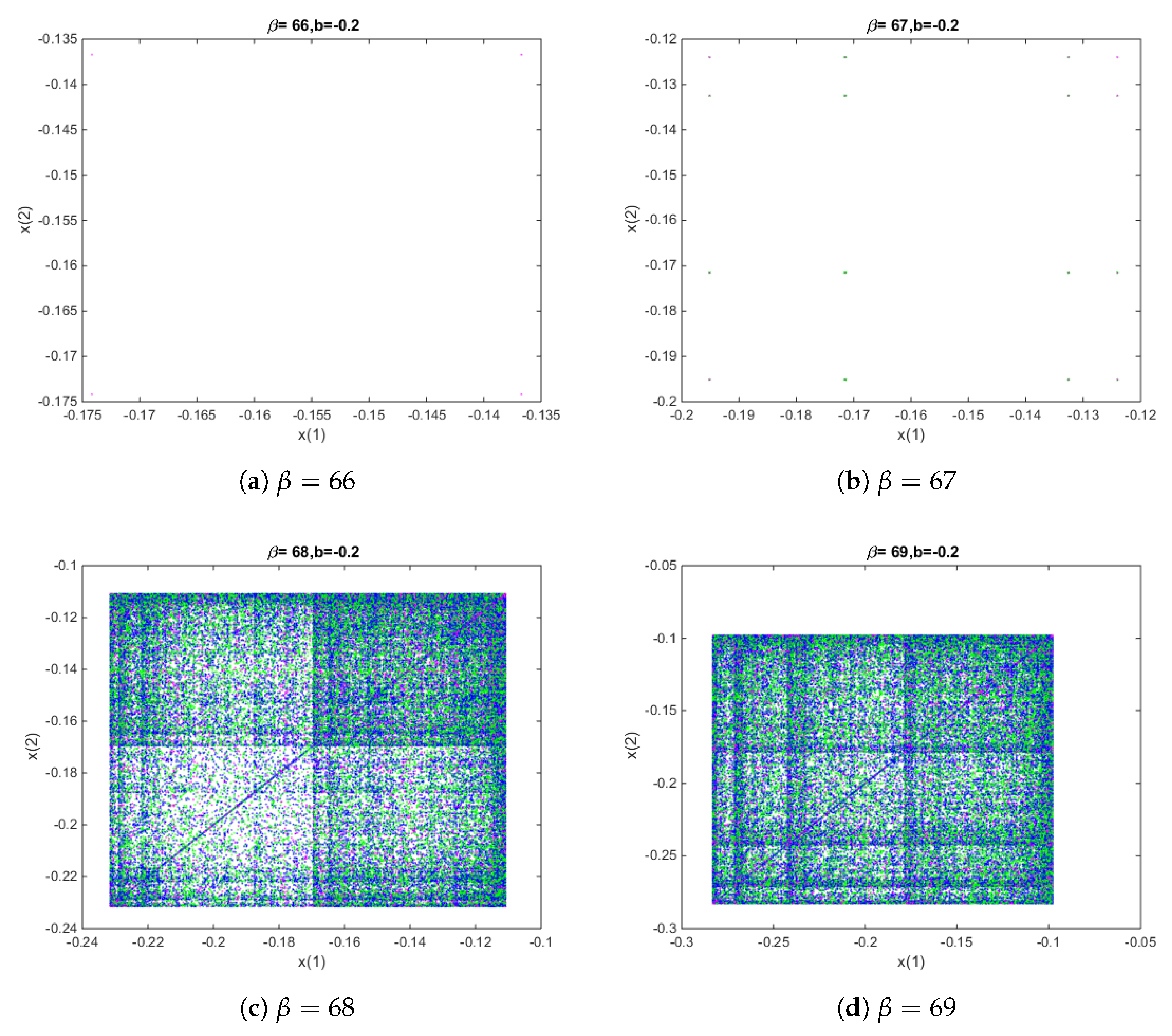
A clear convergent behavior to the roots in the intervals is observed where the critical points are real, except inside the interval $[60,70]$, where a chaotic region can be seen where a strange fixed point has bifurcated (for $\beta =62.0613$, there is change in the number of strange fixed points, two of them parabolic, see Theorem 3) into period-doubling cascades. Further, some blue regions appear associated with chaotic behavior. In them, strange attractors can be found (in the bidimensional case, $n=2$). To do it, we plotted in the $(x_1,x_2)$-space the iteration of $M\left(x_1,x_2\right)$, for values of $\beta$ in the blue area. For each fixed value of parameter $\beta$, 1000 different initial estimations have been used and, for each of them, the iterates have been plotted following this code color: The first 100 iterations are not plotted, while the following 400 are plotted in blue color, the next 400 in green color, and the last hundred in magenta color. This can be observed in Figure 3a,b, as the strange fixed point bifurcates in periodic orbits of increasing period, until the chaotic behavior appears (Figure 3c,d, where the orbits are dense in a small rectangular region of the $x_1,x_2$ space).

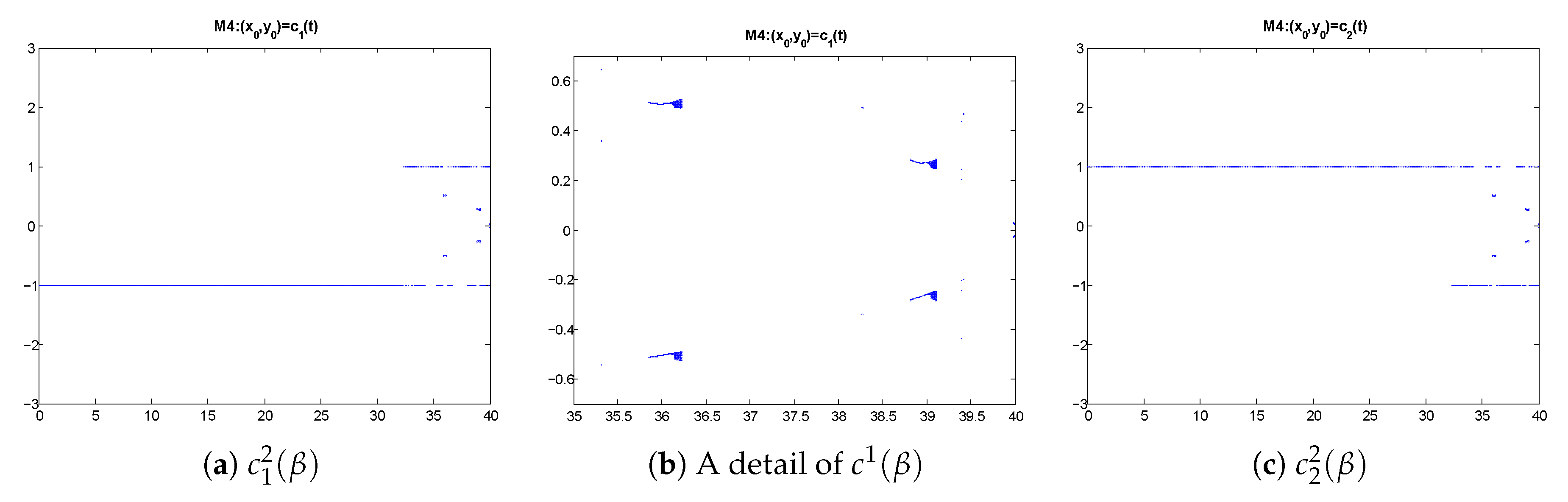
Regarding M42 class, let us remark that there exist only two different free critical points $c_1^2(\beta )=+\sqrt{\frac{-7\beta }{\beta -40}}$ and by $c_2^2(\beta )=-\sqrt{\frac{-7\beta }{\beta -40}}$ (see Theorem 4). In Figure 4a,b, a clear symmetry in the convergence to the roots is observed, and we can also see nonconvergent behavior to the roots for elements corresponding to $\beta \in [35,40]$. 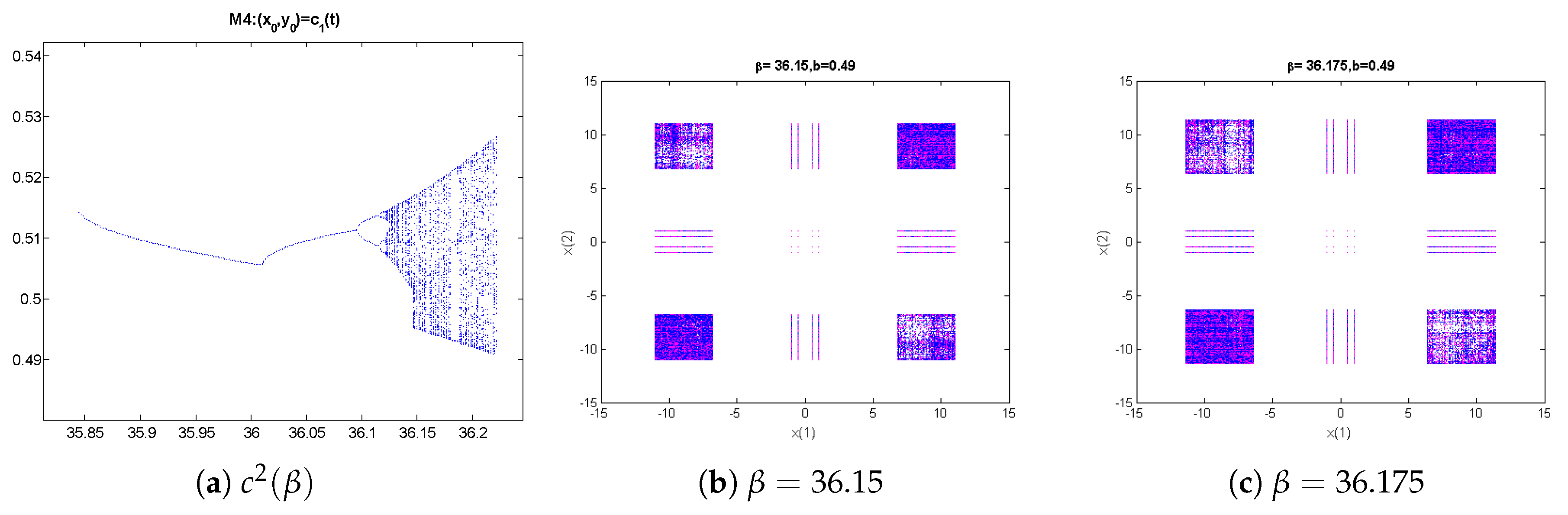We see in Figure 4c four period-doubling bifurcation areas where the repulsive fixed points have bifurcated into period-doubling orbits.

In order to better visualize this behavior, we plotted in the $(x_1,x_2)$-plane the iteration of $M^2\left(x,\beta \right)$, for $\beta$ in the blue area of Figure 5a near to $\beta =36$. Then, symmetric strange attractors appear (see Figure 5b,c).

As in this case, the four strange attractors must be separately identified, the way these pictures have been obtained is slightly different than that used in case M41 family: Fixing the value of parameter $\beta$, 1000 different initial estimations have been taken in small rectangles close to the origin. For each specific value of $\beta$, the method $M^2(x,\beta )$ has been used on each of them, plotting one point per iteration. The code color used is as follows: The first 800 iterations do not appear, while the following 100 appear in blue color and the last hundred are shown in magenta color. The resulting plots show how the four attracting fixed points change into attracting areas, being disjoint or not depending on $\beta$. Nevertheless, the set of starting guesses belonging to their respective basins of attraction is very small, as well as the interval of real values of $\beta$ inducing this performance.

5. Dynamical Planes for $n=2$

In this section, we compare the sensitivity of the proposed classes to the initial estimation, depending on some values of the parameter $\beta$ that have resulted to provide stable or unstable behavior, for each one of the families.

In Figure 6 and Figure 7, we plotted the dynamical planes corresponding to M41 for several values of $\beta$. They were obtained using the routines appearing in Reference [21]. A mesh of $400\times 400$ points was used, the maximum number of iterations employed was 40, and the stopping criterium has a tolerance of ${10}^{-3}$. We plotted a point of this mesh of different colors depending on the root they converge to. Moreover, the color is brighter when the number of iterations used is lower. It is plotted in black color if it reaches the maximum number of iterations without converging to any of the roots.

We observe in Figure 6 that the four roots of the vectorial polynomial have their respective wide basins of attraction (colored in orange, cyan, blue, and purple), with several connected components for each root, separated by the Julia set. There are also four repulsive fixed points and 16 saddle points. In case $\beta =70$, there exist four superattracting fixed points, sixteen repulsive, and other sixteen saddle fixed points. It can be observed in Figure 6b that the number of connected components in the plotted area is much higher, and the immediate basin of attraction (the component holding the fixed point) is smaller in general.

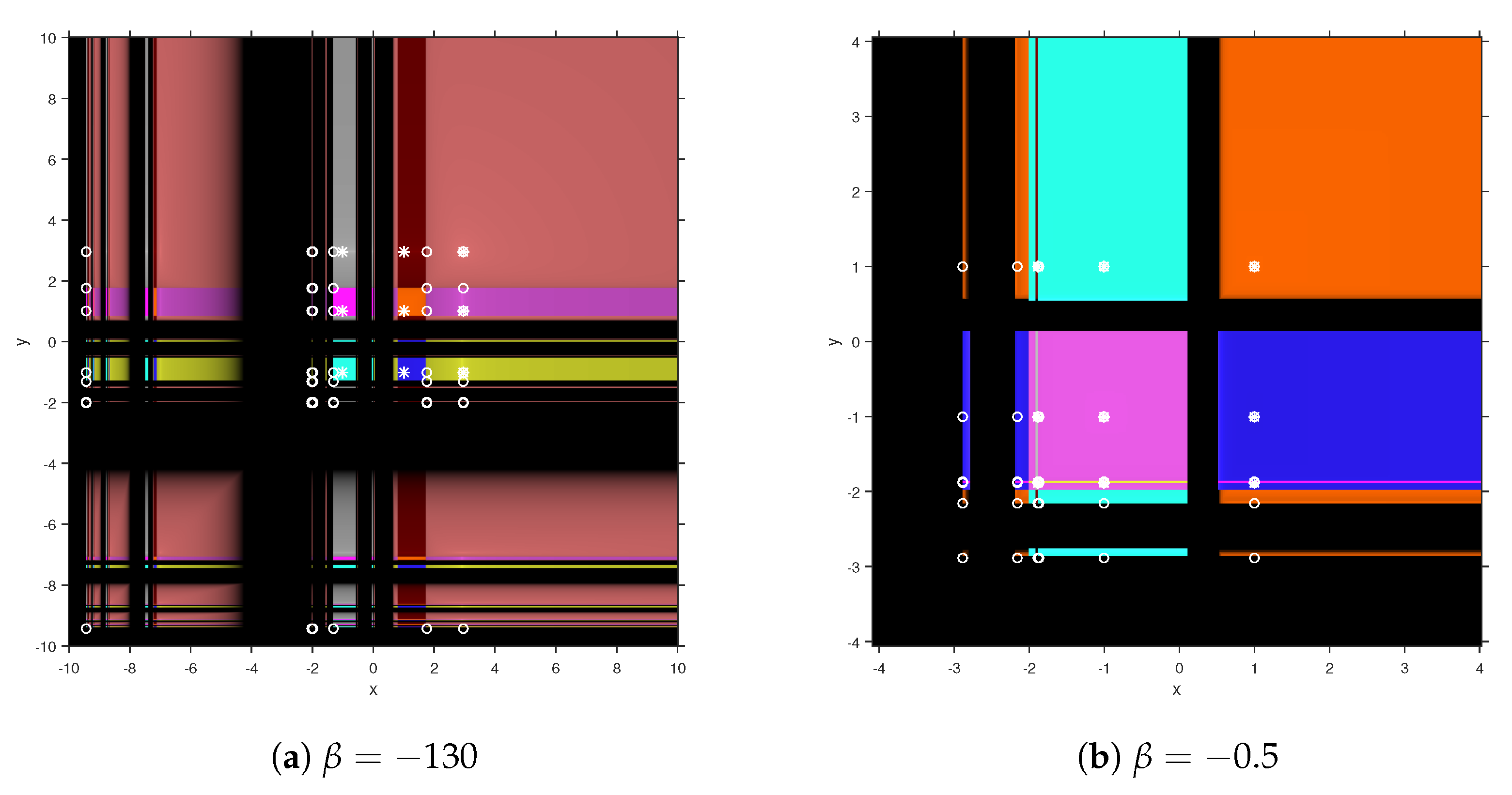
On the other hand, unstable behavior appears in Figure 7, corresponding to the values $\beta =-130$ and $\beta =-0.5$, where nine strange attracting fixed points had been found, in both cases. They are located in the colored areas of no convergence to the roots, presented in yellow, brown, gray, pink, and green, among others. There are also 25 repulsive and 30 saddle fixed points for $\beta =-130$ and, in the case of $\beta =-0.5$, there are 9 repulsive and 18 saddle fixed points. Regarding the symbols, fixed points are marked with a white circle, while those attracting are shown with a white star. Let us remark that repulsive and nonhyperbolic points are always in the Julia set, and attracting ones lay in their respective basin of attraction.

To sum up, the stability of the members of Jacobian-free class M41 of iterative schemes has been analyzed for a quadratic multivariate polynomial. Unstable behavior, in terms of attracting strange fixed points, has been located for $\beta \le -0.4991$, the rest of elements being stable, with wide sets of convergent initial estimations.

Class M42

The dynamical planes related to the M42 class on $p(x)$ for different values of parameter $\beta$ are shown in Figure 8 and Figure 9.

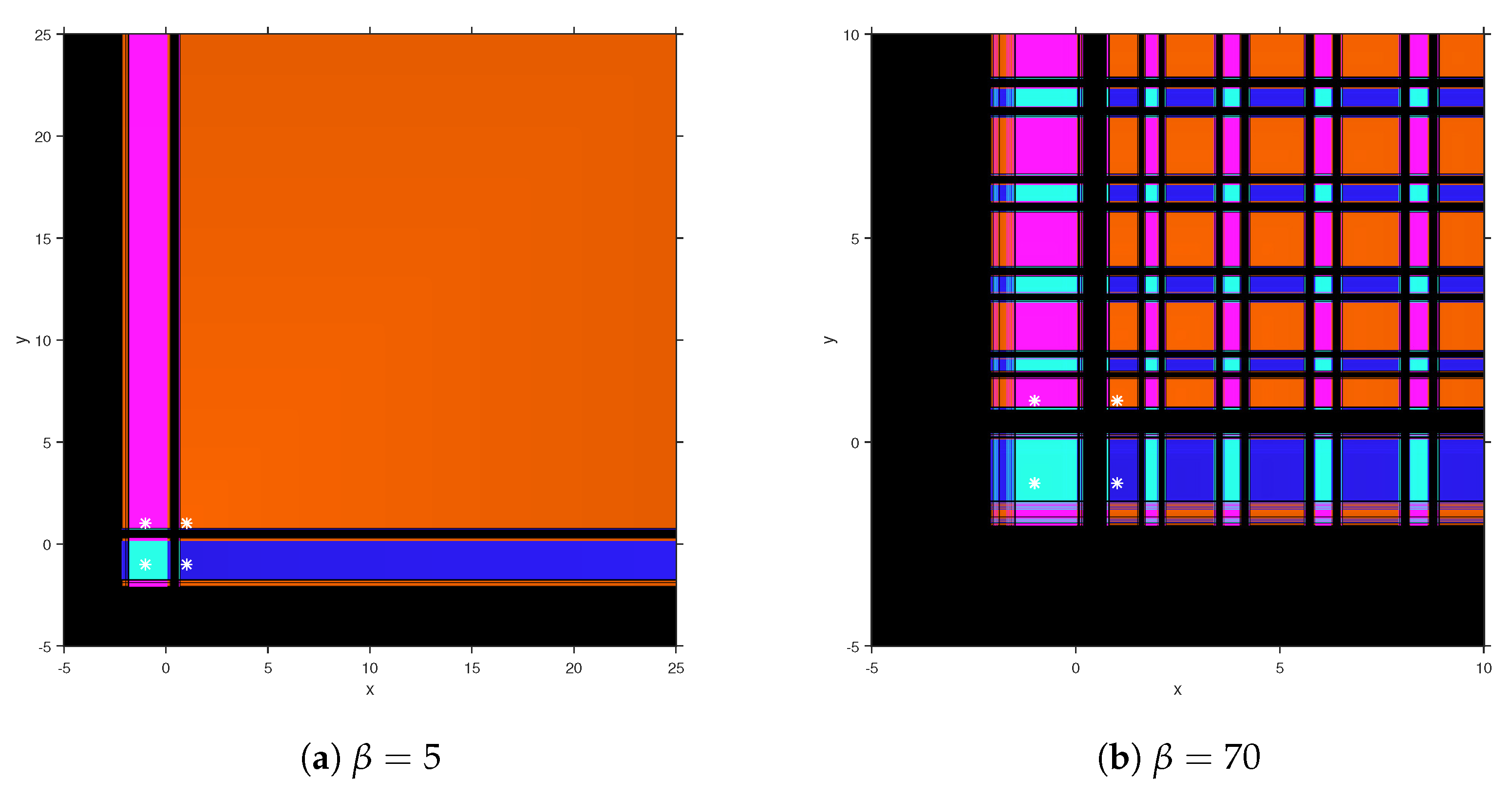
We see in Figure 8a, for $\beta =-10$, that the basins of attraction of the four zeroes of the polynomial form a balanced division of the real plane into four parts (with only a connected component for each root). The fifth-order case $\beta =5$ (Figure 8b) is also stable, but the number of basins of attraction increases slightly with the value of the parameter, and they are divided in several connected components.

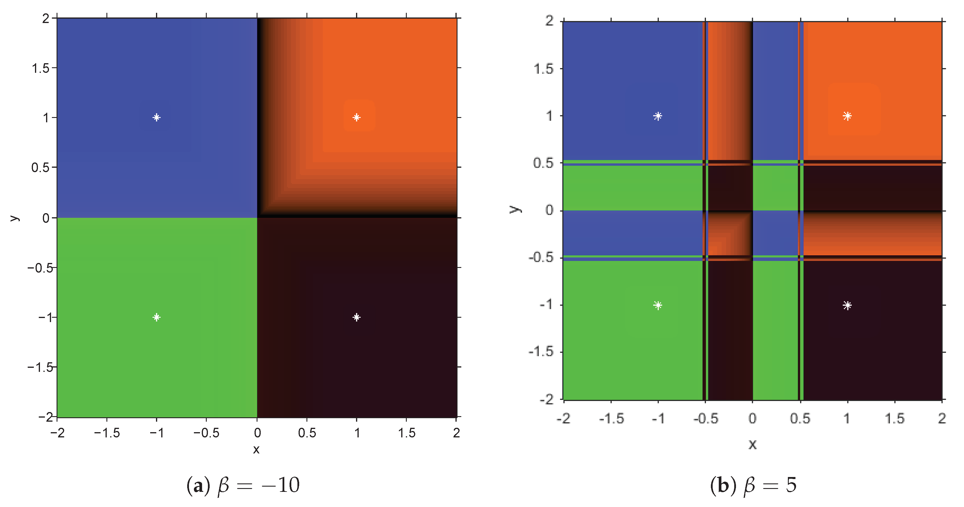
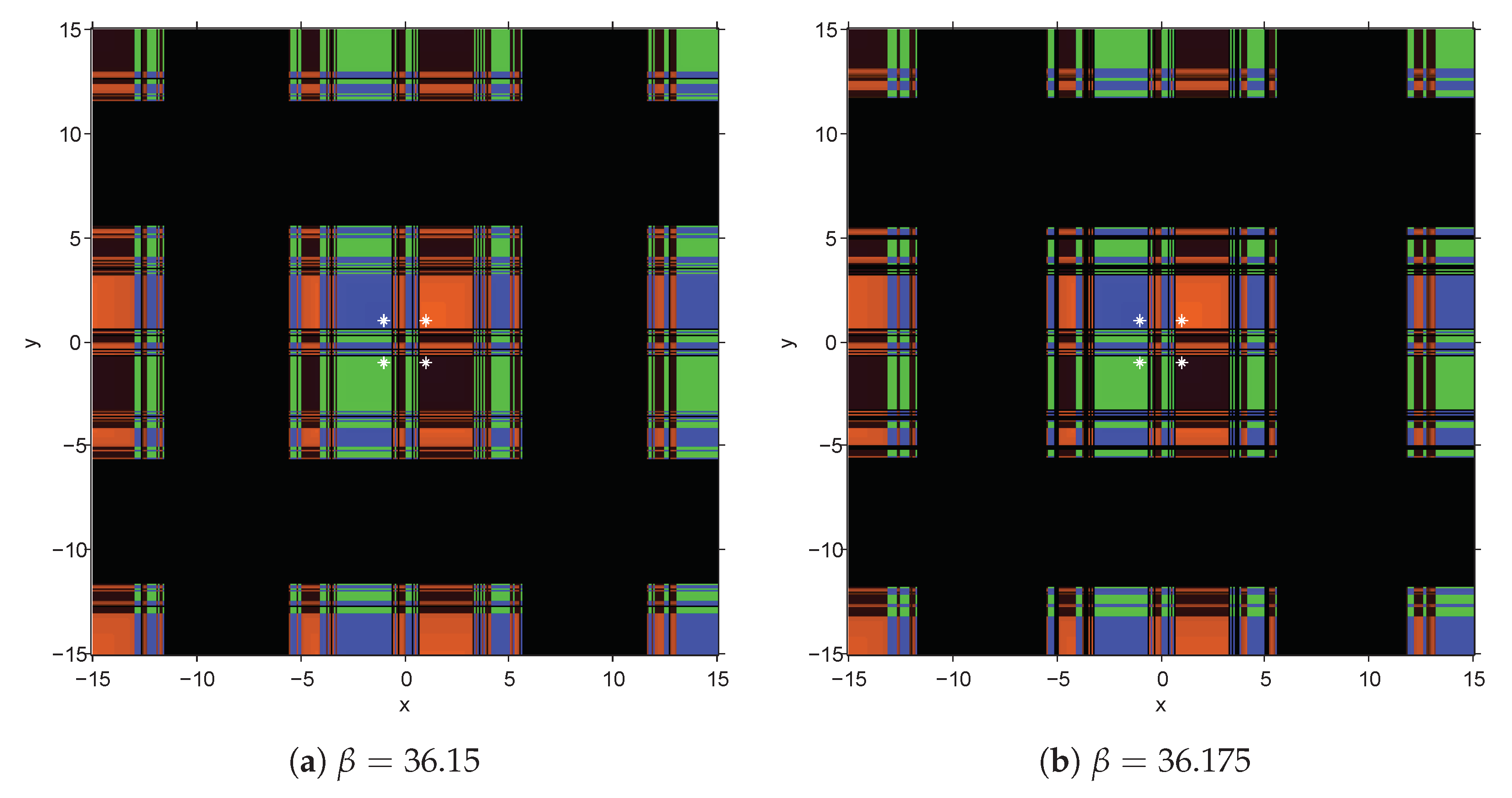
Finally, the unstable behavior is shown in Figure 9a,b, for $\beta =36.15$ and $\beta =36.175$, respectively, where strange attractors appear. They are located in the black regions, showing no convergence to the zeroes.

To summarize, the stability of the elements of classes M41 and M42 of iterative methods were studied for quadratic multivariate polynomial. The only unstable behavior was located in small intervals where attracting periodic orbits or dense attracting regions were found, and the rest of the elements were stable, the most stable ones being clearly stated. This is numerically checked in the following section.

6. Numerical Performance

The numerical results shown in this section were obtained using Matlab R2014b, with variable precision arithmetics with 200 digits of mantissa. In each table of results, the residual $\parallel F(x^{(k)}\parallel$ and the difference between consecutive iterations $\parallel x^{(k)}-x^{(k-1)}\parallel$ are presented for the first three iterations. The approximated computational order of convergence (ACOC) is also calculated, by means of (see [5]):

$$\rho =\frac{ln\left(\left|\right|x^{(k+1)}-x^{(k)}\left|\right|/\left|\right|x^{(k)}-x^{(k-1)}\left|\right|\right)}{ln\left(\left|\right|x^{(k)}-x^{(k-1)}\left|\right|/\left|\right|x^{(k-1)}-x^{(k-2)}\left|\right|\right)}.$$

The nonlinear systems used in these tests, $F(x_1,x_2,\dots ,x_n)=0$, are defined by the following coordinate functions, joint with the corresponding size and the estimated solution to be found:

• $f_i(x_1,x_2,\dots ,x_n)=x_i-cos(2x_i-x_1-x_2-x_3-x_4)$, $i=1,2,\dots ,n$, $n=20$,
  $\overline{x}\approx {(0.5149,0.5149,\dots ,0.5149)}^T$;
• $f_i(x_1,x_2,\dots ,x_n)=x_i-1.5sin\left({\sum }_{j=1}^n{x}_j\right)$, $i=1,2,\dots ,n$, $n=20$,
  $\overline{x}\approx {(0.797242,0.797242,\dots ,0.797242)}^T$.

For each Jacobian-free class, M41 and M42, two stable elements were used ($\beta =5$ and $\beta =10$ for M41 and $\beta =-10$ and $\beta =5$ for M42), and also two respective unstable elements ($\beta =68$ and $\beta =-130$ for M41 and $\beta =36$ and $\beta =36.15$ for M42), expecting to see their performance on nonpolynomial functions.

In both examples of nonpolynomial systems, it is observed that, being good results in general, those obtained using values of parameter $\beta$ that have shown to be stable in the dynamical analysis give more precise results than those that are considered unstable, as can be checked in

Table 1. $f_i(x_1,x_2,\dots ,x_n)=x_i-cos(2x_i-x_1-x_2-x_3-x_4)$, $i=1,2,\dots ,n$, $n=20$, $x^{(0)}={(0.8,0.8,\dots ,0.8)}^T$.

Class	$\mathit{\beta }$	$\parallel {\mathit{x}}^{(1)}-{\mathit{x}}^{(0)}\parallel$	$\parallel \mathit{F}({\mathit{x}}^{(1)})\parallel$	$\parallel {\mathit{x}}^{(2)}-{\mathit{x}}^{(1)}\parallel$	$\parallel \mathit{F}({\mathit{x}}^{(2)})\parallel$	$\parallel {\mathit{x}}^{(3)}-{\mathit{x}}^{(2)}\parallel$	$\parallel \mathit{F}({\mathit{x}}^{(3)})\parallel$	ACOC
M41	5	1.357	0.2225	0.08254	2.895 $\times {10}^{-6}$	1.066 $\times {10}^{-6}$	5.868 $\times {10}^{-26}$	4.0309
M41	10	1.246	0.07772	0.02856	4.087 $\times {10}^{-8}$	1.506 $\times {10}^{-8}$	3.546 $\times {10}^{-33}$	3.9913
M41	68	0.9315	0.9567	0.3453	0.005465	0.002014	2.314 $\times {10}^{-11}$	3.7328
M41	−130	0.8917	1.071	0.3819	0.03454	0.001272	8.167 $\times {10}^{-12}$	3.4626
M42	−10	0.8471	1.1990	0.4278	4.169 $\times {10}^{-6}$	1.536 $\times {10}^{-6}$	1.384 $\times {10}^{-25}$	3.5685
M42	5	1.3470	0.1941	0.07197	5.116 $\times {10}^{-10}$	1.885 $\times {10}^{-10}$	7.685 $\times {10}^{-53}$	4.9915
M42	36	1.0120	0.7287	0.2630	2.376 $\times {10}^{-5}$	8.752 $\times {10}^{-6}$	3.015 $\times {10}^{-22}$	3.7659
M42	36.15	1.0130	0.7261	0.2621	2.391 $\times {10}^{-5}$	8.809 $\times {10}^{-6}$	3.109 $\times {10}^{-22}$	3.7672

and

Table 2. ${\displaystyle f_i(x_1,x_2,\dots ,x_n)=x_i-1.5sin\left(\sum _{j=1}^n{x}_j\right)}$, $i=1,2,\dots ,n$, $n=100$, $x^{(0)}={(0.8,0.8,\dots ,0.8)}^T$.

Class	$\mathit{\beta }$	$\parallel {\mathit{x}}^{(1)}-{\mathit{x}}^{(0)}\parallel$	$\parallel \mathit{F}({\mathit{x}}^{(1)})\parallel$	$\parallel {\mathit{x}}^{(2)}-{\mathit{x}}^{(1)}\parallel$	$\parallel \mathit{F}({\mathit{x}}^{(2)})\parallel$	$\parallel {\mathit{x}}^{(3)}-{\mathit{x}}^{(2)}\parallel$	$\parallel \mathit{F}({\mathit{x}}^{(3)})\parallel$	ACOC
M41	5	1.233 $\times {10}^{-2}$	3.827 $\times {10}^{-5}$	1.522 $\times {10}^{-6}$	4.672 $\times {10}^{-18}$	1.858 $\times {10}^{-19}$	1.039 $\times {10}^{-69}$	4.0
M41	10	0.01233	2.747 $\times {10}^{-5}$	1.093 $\times {10}^{-6}$	9.852 $\times {10}^{-19}$	3.919 $\times {10}^{-20}$	1.629 $\times {10}^{-72}$	4.0
M41	68	1.237 $\times {10}^{-2}$	8.575 $\times {10}^{-4}$	3.411 $\times {10}^{-5}$	1.913 $\times {10}^{-12}$	7.608 $\times {10}^{-14}$	4.684 $\times {10}^{-47}$	4.0005
M41	−130	1.228 $\times {10}^{-2}$	1.434 $\times {10}^{-3}$	5.704 $\times {10}^{-5}$	5.968 $\times {10}^{-11}$	2.374 $\times {10}^{-12}$	1.82 $\times {10}^{-40}$	3.9990
M42	−10	1.212 $\times {10}^{-2}$	5.273 $\times {10}^{-3}$	2.097 $\times {10}^{-4}$	7.529 $\times {10}^{-13}$	2.994 $\times {10}^{-14}$	6.357 $\times {10}^{-52}$	3.9687
M42	5	1.293 $\times {10}^{-2}$	1.492 $\times {10}^{-2}$	5.94 $\times {10}^{-4}$	8.504 $\times {10}^{-12}$	3.382 $\times {10}^{-13}$	2.075 $\times {10}^{-60}$	5.2587
M42	36	1.367 $\times {10}^{-2}$	3.346 $\times {10}^{-2}$	1.333 $\times {10}^{-3}$	4.298 $\times {10}^{-8}$	1.709 $\times {10}^{-9}$	1.395 $\times {10}^{-32}$	4.1567
M42	36.15	1.367 $\times {10}^{-2}$	3.347 $\times {10}^{-2}$	1.333 $\times {10}^{-3}$	4.325 $\times {10}^{-8}$	1.72 $\times {10}^{-9}$	1.438 $\times {10}^{-32}$	4.1569

.

7. Conclusions

Two highly efficient Jacobian-free classes of iterative methods were designed, and it has been proven that their order of convergence is four, except for a fifth-order particular case at $\beta =5$ for the second class. The real multidimensional stability of the members of both classes of iterative schemes was analyzed for quadratic $n\times n$ polynomial systems. For the first family, only two real components of strange fixed points that can yield attracting points different from the roots appear. In the second one, there are no attracting strange fixed points. On the other hand, free real critical points fall in chaotic behavior only in small intervals for both cases. The rest of the members are stable, being the most similar performance to Newton’s scheme located around $\beta =5$. Finally, numerical experiments confirm the theoretical results, showing good performance in all cases but having lower residual errors in those cases that correspond to the stable values of the parameter.

References

- Frontini, M.; Sormani, E. Third-order methods from quadrature formulae for solving systems of nonlinear equations. Appl. Math. Comput. 2004, 149, 771–782. [Google Scholar] [CrossRef]
- Homeier, H.H.H. A modified Newton method with cubic convergence: The multivariable case. J. Comput. Appl. Math. 2004, 169, 161–169. [Google Scholar] [CrossRef]
- Noor, M.A.; Waseem, M. Some iterative methods for solving a system of nonlinear equations. Comput. Math. Appl. 2009, 57, 101–106. [Google Scholar] [CrossRef]
- Xiao, X.; Yin, H. A new class of methods with higher order of convergence for solving systems of nonlinear equations. Appl. Math. Comput. 2015, 264, 300–309. [Google Scholar] [CrossRef]
- Cordero, A.; Torregrosa, J.R. Variants of Newton’s method using fifth-order quadrature formulas. Appl. Math. Comput. 2007, 190, 686–698. [Google Scholar] [CrossRef]
- Darvishi, M.T.; Barati, A. A third-order Newton-type method to solve systems of nonlinear equations. Appl. Math. Comput. 2007, 187, 630–635. [Google Scholar] [CrossRef]
- Sharma, J.R.; Guha, R.K.; Sharma, R. An efficient fourth order weighted-Newton method for systems of nonlinear equations. Numer. Algor. 2013, 62, 307–323. [Google Scholar] [CrossRef]
- Narang, M.; Bhatia, S.; Kanwar, V. New two-parameter Chebyshev-Halley-like family of fourth and sixth-order methods for systems of nonlinear equations. Appl. Math. Comput. 2016, 275, 394–403. [Google Scholar] [CrossRef]
- Behl, R.; Sarría, I.; Crespo, R.G.; Magreñán, Á.A. Highly efficent family of iterative methods for solving nonlinear models. Comput. Appl. Math. 2019, 346, 110–132. [Google Scholar] [CrossRef]
- Amorós, C.; Argyros, I.K.; González, R.; Magreñán, Á.A.; Orcos, L.; Sarría, I. Study of a high order family: Local convergence and dynamics. Mathematics 2019, 7, 225. [Google Scholar] [CrossRef]
- Argyros, I.K.; González, D. Local convergence for an improved Jarratt-type method in Banach space. IJIMAI 2015, 3, 20–25. [Google Scholar] [CrossRef]
- Sharma, J.R.; Gupta, P. An efficient fifth order method for solving systems of nonlinear equations. Comput. Math. Appl. 2014, 67, 591–601. [Google Scholar] [CrossRef]
- Cordero, A.; Torregrosa, J.R.; Vassileva, M.P. Design, Analysis, and Applications of Iterative Methods for Solving Nonlinear Systems. In Nonlinear Systems—Design, Analysis, Estimation and Control; InTechOpen: London, UK, 2016; Chapter 5; pp. 87–116. [Google Scholar]
- Cordero, A.; Gutiérrez, J.M.; Magreñán, Á.A.; Torregrosa, J.R. Stability analysis of a parametric family of iterative methods for solving nonlinear models. Appl. Math. Comput. 2016, 285, 26–40. [Google Scholar] [CrossRef]
- Cordero, A.; Chicharro, F.I.; Torregrosa, J.R. Real stability of an efficient family of iterative methods for solving nonlinear systems. In Proceedings of the Conference CEDYA + CMA 2017, Cartagena, Spain, 26–30 June 2017; pp. 213–218. [Google Scholar]
- Robinson, R.C. An Introduction to Dynamical Systems, Continous and Discrete; Americal Mathematical Society: Providence, RI, USA, 2012. [Google Scholar]
- Cordero, A.; Soleymani, F.; Torregrosa, J.R. Dynamical analysis of iterative methods for nonlinear systems or how to deal with the dimension? Appl. Math. Comput. 2014, 244, 398–412. [Google Scholar] [CrossRef]
- Cordero, A.; Hueso, J.L.; Martínez, E.; Torregrosa, J.R. A modified Newton-Jarratt’s composition. Numer. Algor. 2010, 55, 87–99. [Google Scholar] [CrossRef]
- Ortega, J.M.; Rheimboldt, W.C. Iterative Solutions of Nonlinear Equations in Several Variables; Academic Press: New York, NY, USA, 1970. [Google Scholar]
- Argyros, I.K.; George, S. Ball convergence for Steffensen-type fourth-order methods. IJIMAI 2015, 3, 37–42. [Google Scholar] [CrossRef]
- Chicharro, F.I.; Cordero, A.; Torregrosa, J.R. Drawing dynamical and parameters planes of iterative families and methods. Sci. World 2013, 2013, 780153. [Google Scholar] [CrossRef] [PubMed]
Figure 1.
Stability of the fixed points.
Figure 2.
Feigenbaum diagrams of , .
Figure 3.
Strange attractors of M41 class for values in the period-doubling cascade region.
Figure 4.
Figure 5.
Strange attractors of M42 class for values in the period-doubling cascade region.
Figure 6.
Dynamical planes for stable values of of class M41 on .
Figure 7.
Dynamical plane for unstable values of of class M41 on .
Figure 8.
Dynamical planes for stable values of of class M42 on .
Figure 9.