1. Introduction
Journal bearings are used in industrial applications to support the rotors in rotating machineries. This includes the use of this type of bearings in compressors and various types of turbines, such as gas, hydroelectric, and steam turbines, in addition to many other applications. Such a wide range of use is attributed to their high load, damping, operating speed, and relatively low manufacturing and maintenance cost. The industrial demand for high-power output leads to a more increase in the rotating machinery speed. However, operating at a high level of speed may result in large unstable oscillations related to the self-excited vibrations. This type of instability may lead to severe damage to the bearing. Therefore, predicting the onset of instability represents an essential step in designing this type of bearing for a safe operation [
1]. Unbalance excitation is one of the rotor-bearing system’s most important causes of vibration. Unbalance, in fact, is a common machinery fault that results in due to the uneven mass distribution of any rotating machine element about its axis [
2]. The vibration resulting from this type of excitation usually causes noise and may decrease the life of the bearings as well as result in unsafe working conditions [
3]. These important aspects of the unbalance in the rotor bearing system have resulted in considerable literature being published on this topic over the last decades. One of the early works related to the effect of unbalance on the performance of a short bearing was presented by [
4], but the results of the theory of short bearing involve significant errors when the bearing length to diameter ratio of the bearing is larger than 0.5 [
5]. Brancati et al. [
6] also analyzed an unbalanced rotor supported by journal bearings based on the use of the short bearing theory for different values of dimensionless unbalance of the rotor. As the unbalance is inherently present in any rotor and it is important to be considered in the modeling, Adiletta et al. [
7,
8,
9] used numerical and experimental investigations to study the effect of unbalance on rotor response and examined the conditions for which chaotic motion may exist. However, the analyses were limited to specific bearing and rotor conditions. Chang-Jiang and Chen [
10] used a simplified model to study the effect of rotating unbalance on the system’s response using long journal bearings. El-Saeidy and Sticher [
11] presented a formulation for the dynamic analysis of rigid rotors subject to the mass imbalance in addition to base excitations. Sghir and Chouchane [
1] investigated a wide domain of rotor bearing (short bearing) conditions where the effect of unbalance on the system response is investigated in each case. Their results illustrated that, in comparison with the perfectly balanced system, the unbalance might cause periodic oscillations at different speed ranges at multiple periods of rotation and even chaotic motion. Recently, Eling et al. [
12] presented an interesting work on predicting the unbalance response of rotors supported on journal bearings considering unbalance force. They explained the interaction between the rotating shaft and the oil film that can result in unstable dynamic behavior characterized by sub-synchronous motion, the oil whirl, where the whirl frequency in journal bearing is close to half the rotation speed.
In addition to the problem of unbalance excitation, the system’s general performance is also greatly influenced by the presence of misalignment. In the typical use of journal bearing, the shaft is subjected to some degree of deviation with respect to the bearing axis due to many causes, such as the shaft deflection and the errors resulting from inappropriate installation or manufacturing, as well as the bearing wear. Researchers have illustrated the negative effects of the misalignment on the journal bearing performance [
13,
14,
15,
16,
17,
18] in terms of reducing the thickness of the oil layer that separates the journal and the bearing and the increase in the level of the pressure field in addition to the possibility of reducing bearing life as a result of the increase in the friction coefficient. These negative consequences can be reduced by modifying the bearing profile to compensate for the reduction in the separated clearance between the journal and the bearing. This geometrical design development is investigated by researchers considering different aspects. Optimizing the bearing geometry, for example, was experimentally investigated by Nacy [
19] in order to control the side leakage using chamfered bearing edges. Another attempt in this direction was performed by [
20], where they used defects in the bearing geometry in order to study its effects on reducing misalignment consequences on the bearing performance. Instead of performing localized modification of the bearing profile, Strzelecki [
21] changed the bearing profile over the whole length using a hyperboloidal profile in order to increase the load-carrying capacity under misalignment. Chasalevris and Dohnal [
22] showed that the stability of the journal-bearing system can be improved based on the use of variable geometry. Recently, Ren et al. [
23] used a numerical investigation to study the effects of profile parameters on the bearing performance, where the results showed that the quadratic profile improves the bearing performance significantly. Jamali et al. [
24,
25] showed that the bearing performance can be improved by using a variable bearing profile. More recently, the misalignment problem in journal bearing has also been investigated by [
26,
27,
28]. However, all these works did not consider the effect of changing the geometrical bearing profile parameters on the system response to unbalance excitations.
This work investigates the problem of unbalanced excitation of a rotor supported on finite-length journal bearings considering variable geometrical design parameters of the bearing profile. The effects of varying these parameters on the system’s characteristics in the case of 3D shaft deviation will be examined first in terms of the resulting level of film thickness and severity of the pressure spikes resulting from this 3D form of deviation. Then, the model will evaluate these geometrical modifications’ effectiveness on the rotor-bearing system’s unbalance response under a wide range of unbalanced excitations and rotational speeds. The finite difference method is considered in the discretization scheme of the governing equations using the Reynolds boundary conditions method. On the other hand, the 4th order Range Kutta method is used for solving the journal equations of motion that required identifying the shaft center trajectories under different operating and design conditions.
2. Governing Equations and the Mathematical Model
The required equations for the solution of finite length misaligned bearing with the consideration of bearing profile modification are presented in this section, and their numerical solution will be illustrated later.
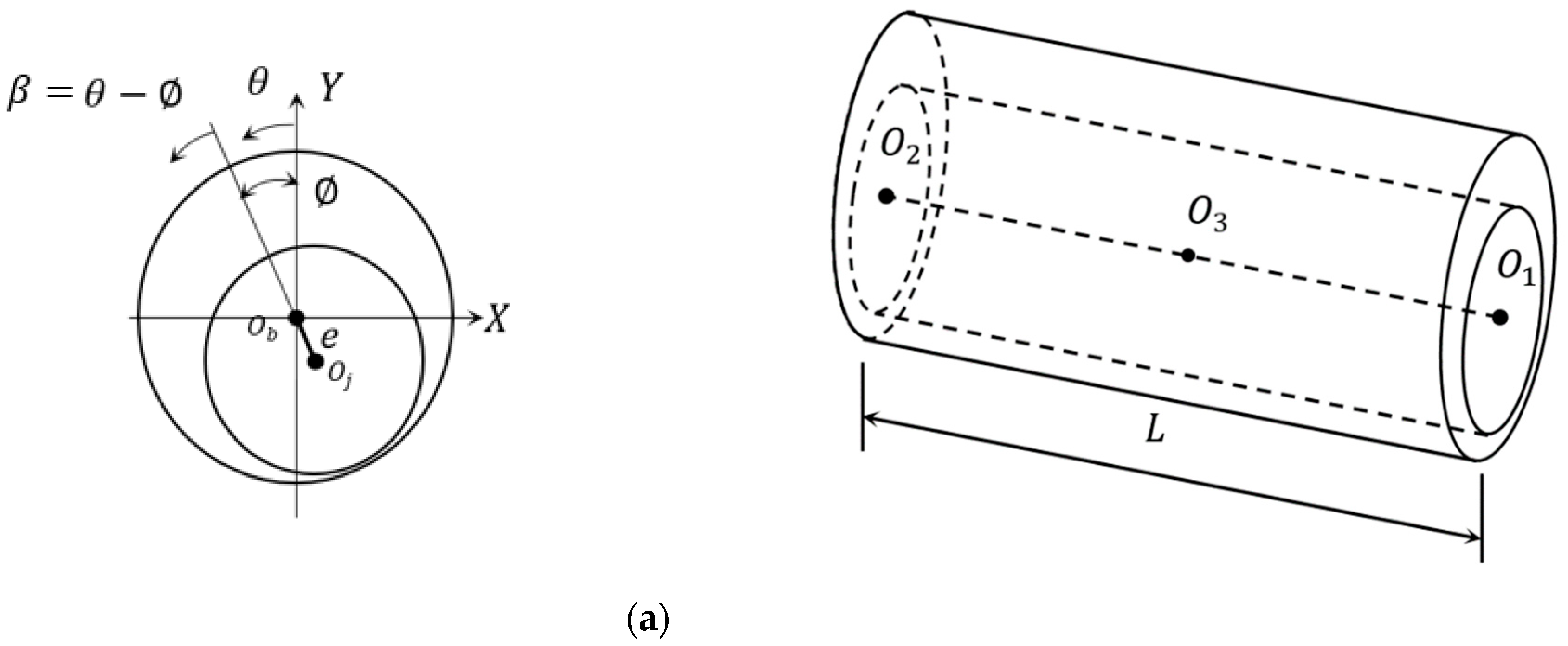
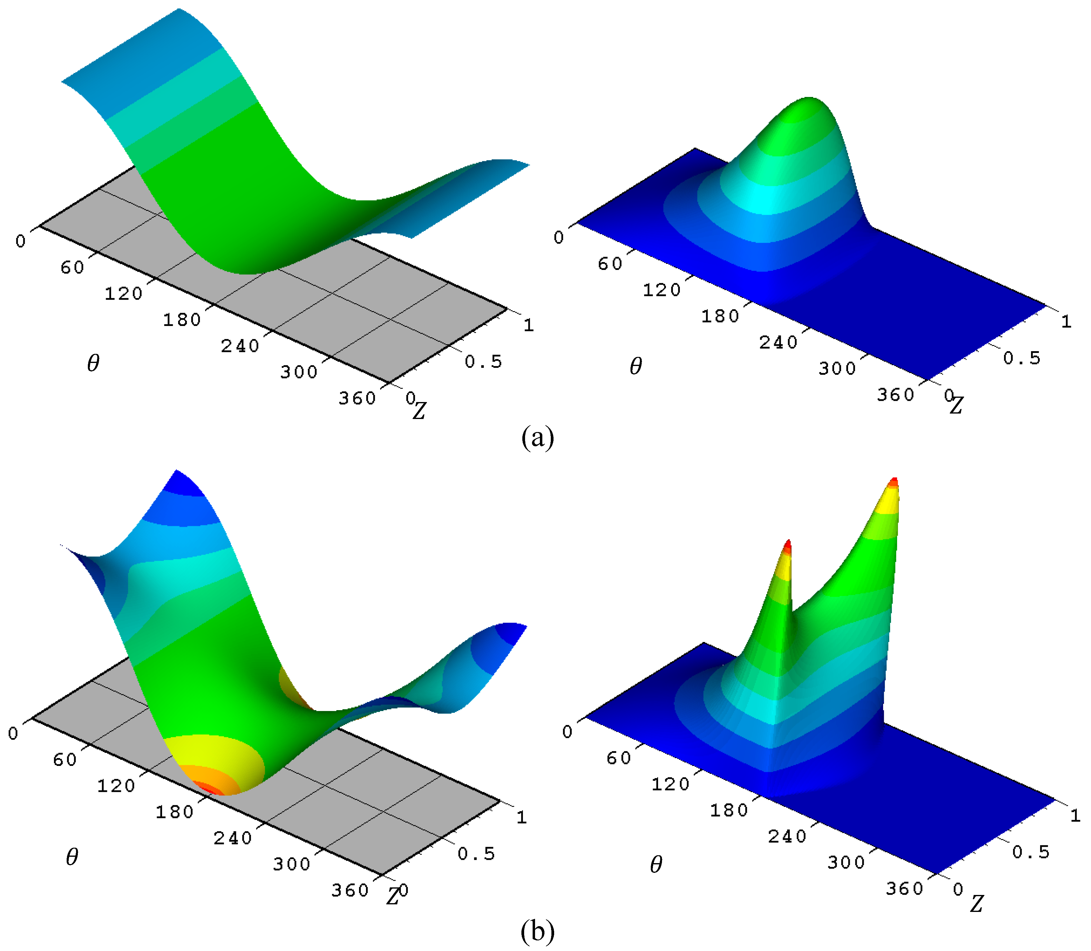
Figure 1 shows schematics drawings for the adopted model of the solution, whereas
Figure 1a illustrates two views for the ideal case (without misalignment) of the bearing.
Figure 1c shows the misaligned model, and
Figure 1c explains the geometrical modification of the bearing profile. All the variables in this figure will be explained in more detail and the related equations.
Reynolds equation is the main equation that governs the solution of the hydrodynamic problem of journal bearing. This equation and the film thickness equation are given by [
17,
29],
where,
: viscosity and density of the lubricant, respectively.
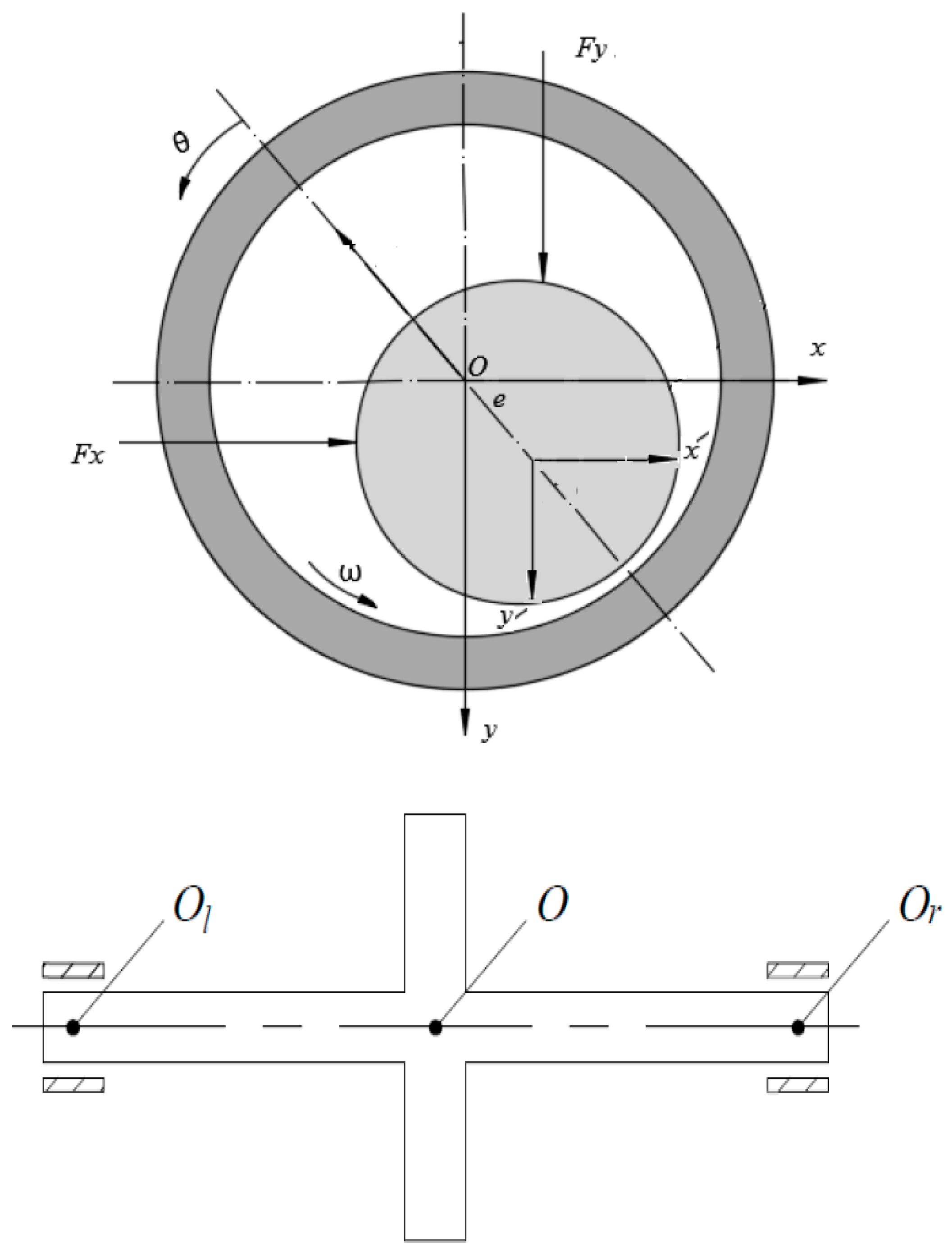
: mean entraining velocity, which is given by , and are the journal and bearing speed where and
p: pressure
h: film thickness
: attitude angle
t: time
c: radial clearance
: eccentricity ratio, which is given by, where is eccentricity distance
Equation (1) is solved using Reynolds boundary conditions where the following conditions are used [
30]:
where
is the cavitation angle which is determined using an iterative solution [
30,
31].
Using the following variables, Equations (1) and (2) can be written in dimensionless forms:
where,
The dimensionless forms of Equations (1) and (2) are:
where:
The dimensionless supported load is given by
where,
and
And the attitude angle is [
32].
The 3D misalignment model (
Figure 1b) is adapted from the work of the first author [
17], where the following equations govern this model:
where, and
and
(dimensionless variables)
This 3D misalignment model represents a more realistic model for the vertical ( and horizontal deviations of the shaft.
In contrast with the ideal case of the journal bearing, the attitude angle, as well as the eccentricity in the misaligned case, are not constant along the bearing length, and they are functions of the position
Z [
17],
where,
: attitude angle at
: eccentricity at
Using these equations, the resulting gap due to the presence of 3D misalignment can be calculated.
The variation of the bearing profile shown previously in
Figure 1c will change the gap between the shaft’s surface and the bearing’s inner surface, which is essentially used to compensate for the reduction in the gap due to misalignment. Detailed steps of this method were explained in [
24].
The modification of the bearing profile consists of removing material from the inner surface of the bearing in order to overcome the negative consequences of the 3D misalignment (misalignment in the vertical and horizontal directions), which mainly causes a thinning in the gap between the shaft (journal) and the bearing. This modification is governed by two parameters which are the length along the longitudinal bearing direction where the modification is performed (
) and the distance in the radial direction (
). These two parameters are illustrated in
Figure 1c and will be written in a dimensionless form for generality, as will be explained later.
The resulting gap due to bearing profile modification (function of
Z) can be given by,
where
and
are:
=
and
(
a and
b are illustrated in
Figure 1c)
The advantages of using a variable bearing profile can be evaluated based on the A and B parameters. These parameters (dimensionless) are given in terms of the (the radial clearance) and (the width of the bearing), which gives a more obvious understanding of the required geometrical change of the profile to minimize the 3D deviation negative effects.
The total gap considering the misalignment and the variable bearing profile can be determined by coupling the related equations (Equations (4), (9) and (11)).
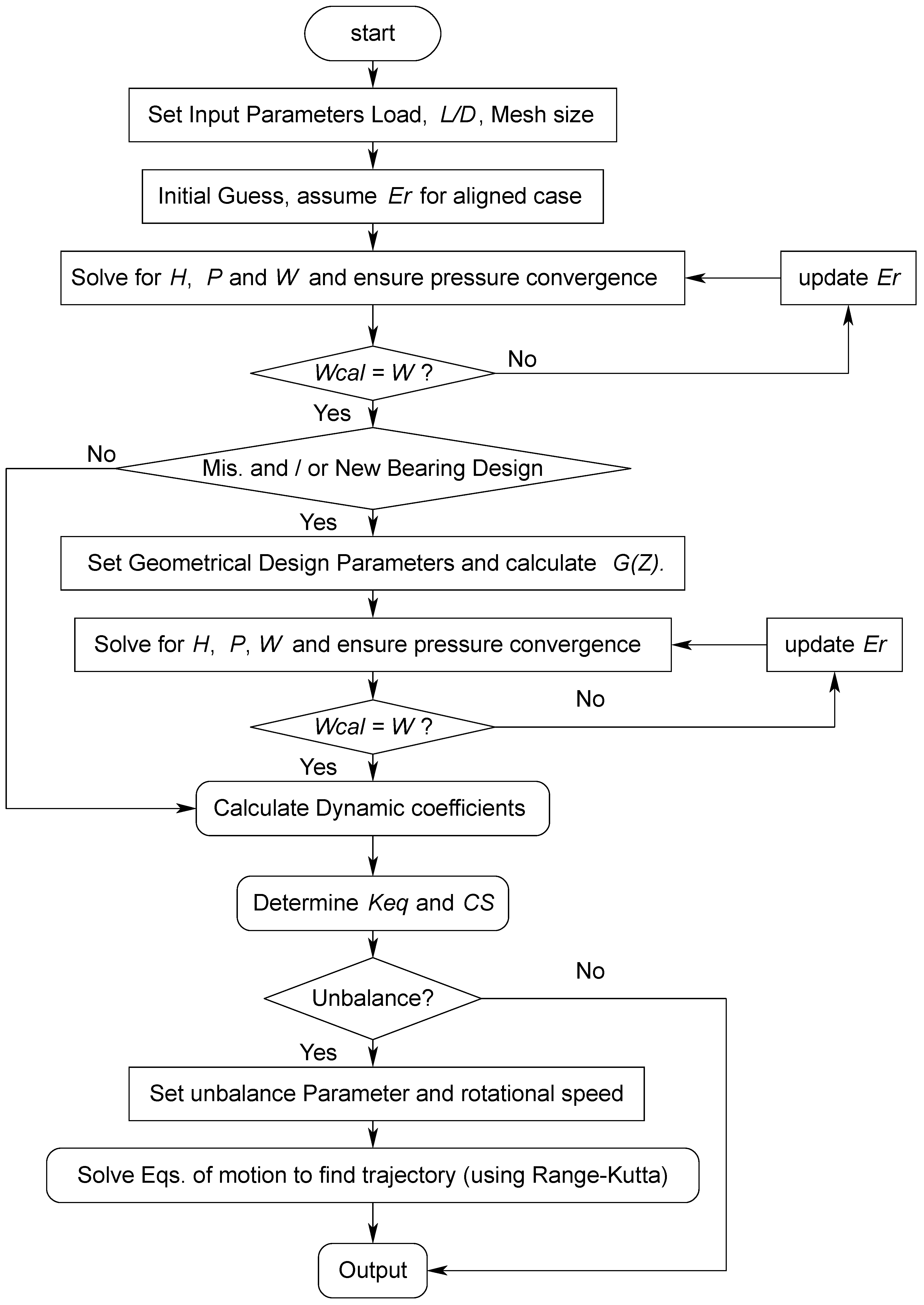
5. Numerical Solution
At first, the pressure field is obtained by discretizing the Reynolds equation, using the finite difference method, and the related equations for determining the gap between the two surfaces: the equations of film thickness, the 3D deviation, and the profile modification. The method of successive over-relaxation is considered in the solution under the use of the Gauss-Sedial method. These pressure fields are obtained by determining the stiffness and dynamic coefficients by numerical integration. Then, the equations of motion are solved numerically using a fourth-order Runge-Kutta method.
Discretizing the governing equations yields,
where,
, , , and are the mesh steps.
More details about the discretization and the solution steps can be found in [
17]. After discretizing Equations (22)–(25), the pressure derivative required to calculate the dynamic coefficients is given by,
where,
and the other constants are as defined previously.
The RHS of Equations (22)–(25) is calculated numerically as follows:
After discretizing all the related equations, the numerical solution is performed where the converges criterion for the pressure is, .
The hydrodynamic load is calculated by numerical integration after determining the pressure field. This load is compared with the actual load, and the solution is accepted if an accuracy of
is achieved (
is within the range of
). If this limit is <
, the solution requires a very long computational time without any significant change in the static and dynamic results. If this accuracy is not achieved (
, the eccentricity ratio
is updated, and the whole process is repeated where the pressure distribution and the gap between the surfaces are recalculated; this step results in new values for the dynamic coefficients. After achieving both convergences (
P and
W), the equations of motion are solved using the 4th-order Range-Kutta method, as explained previously. A flow chart for the main steps of the solution procedure is illustrated in
Figure 3.
6. Results and Discussions
The results in this work are presented considering finite length journal bearing where the length-to-diameter ratio
is 1.25, and the load is corresponding to the case of a perfectly aligned bearing with a typical value of the eccentricity ratio
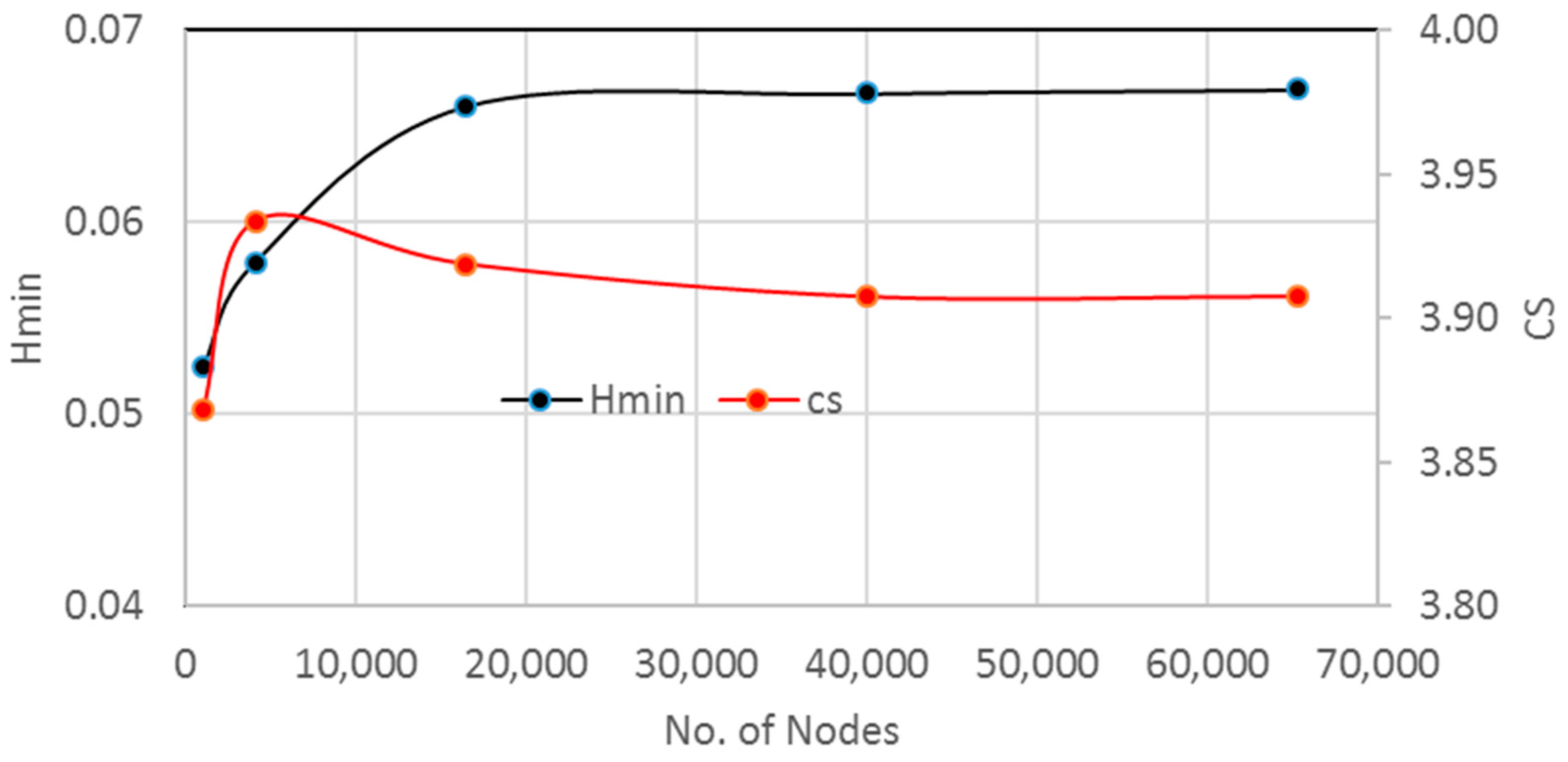
as 0.6. In order to better understand the geometrical design importance on the dynamic behavior of the rotor-bearing system, at first, the results will be focused on the resulting film thickness and pressure distributions due to the bearing variable geometry. Then, the investigation will be further advanced to explain in detail the effect of geometrical design parameters on the shaft trajectories under different unbalanced conditions. This sequence of presenting will give a clearer picture of the significance of the bearing profile design parameters on the system’s static and dynamic characteristics. The first step in performing the numerical solution, the independency of the results on the number of nodes, is examined as shown in
Figure 4. In this figure, the values of the dimensionless minimum film thickness (H
min) and the dimensionless critical speed (CS) are plotted against the number of nodes. It can be seen that increasing the number of nodes
beyond 16,471 has a trivial effect on both results despite the narrow range of the y-axes of H
min and CS. Therefore, this number is adopted in this analysis. Furthermore, the current model is also verified using the results presented by reference [
22], as shown in
Table 1. A relatively low and high value of the Summerfield numbers is used in the comparison shown in this table. It can be seen that very good agreements are found for the values of
and
for the two Summer field numbers.
As the ideal case of a perfectly aligned bearing rarely exists in the typical applications of the journal bearings, as explained previously, the presence of misalignment is well known to have negative consequences on the general system performance. The misalignment significantly affects the film thickness, the pressure distributions, and their shape variation. Using a variable geometry for the bearing profile has the advantage of minimizing these negative effects on the system characteristics.
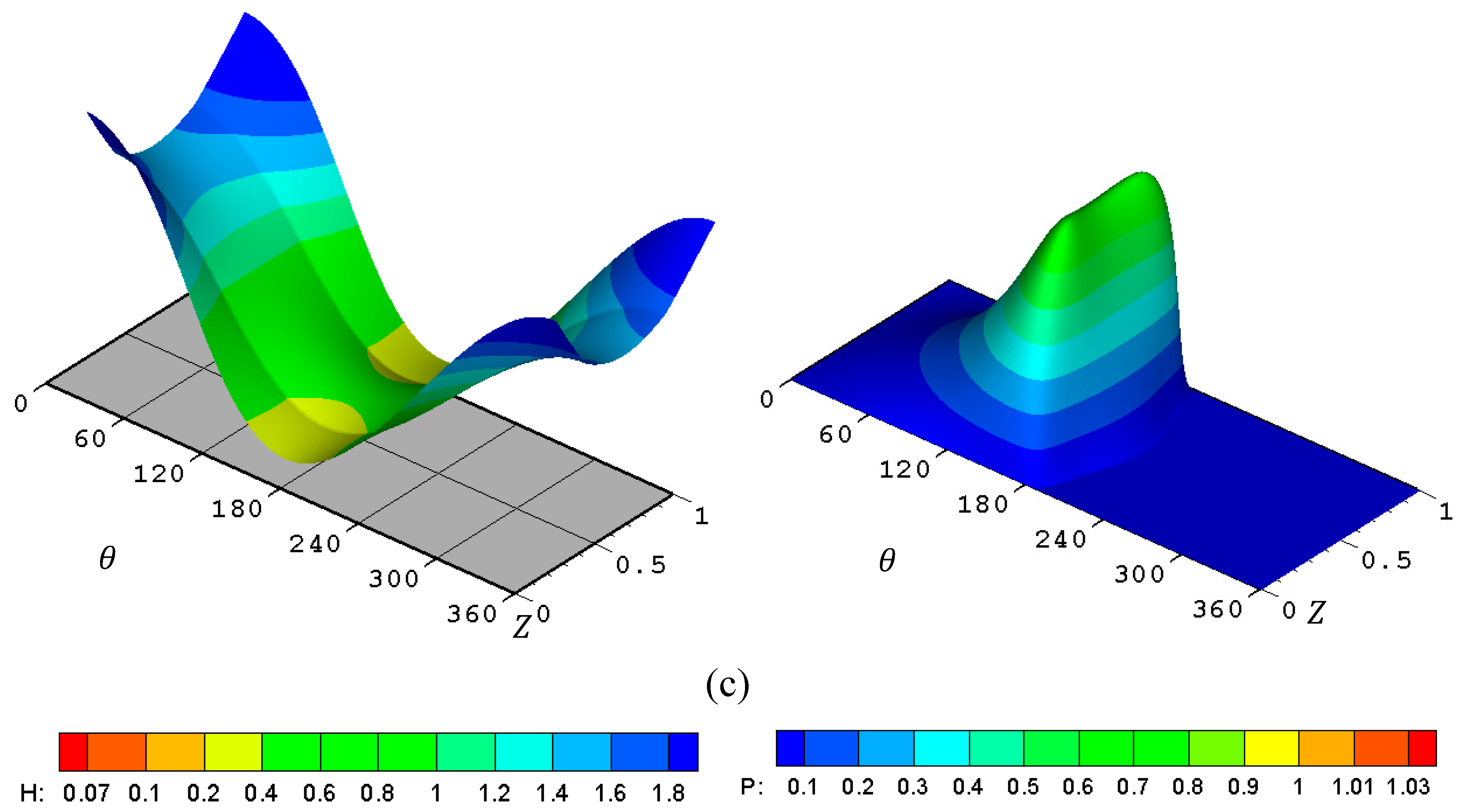
Figure 5 shows the dimensionless film thickness and the dimensionless pressure distribution for three cases of the finite-length journal bearing.
Figure 5a–c show the results for the ideal case of aligned bearing, the misaligned bearing under 3D misalignment, and the case of misaligned bearing with a modified geometry, respectively. Sever levels of misalignment are used in the case of 3D misalignment in order to illustrate how the modification can improve the bearing performance. The film thickness in the aligned case is prismatic, where the value of the film thickness at any circumferential position is constant along the bearing width. On the other hand, the pressure distribution is symmetric about the middle of the bearing width. The H
min and P
max values for this case are 0.4 and 0.645, respectively. The presence of the misalignment increases P
max by 63.8% to 1.057 and reduces H
min by 85.7% to 0.0572, representing a significant change in the designed values of the system. In addition, the film thickness distribution is no longer prismatic, and the pressure distribution is not symmetric about the middle axis of the bearing. Such a level of minim film thickness reduces the bearing life due to the expected high friction and wear ranges. In order to overcome this problem, the load-carrying capacity of the bearing should be reduced significantly to increase the value of the minimum film thickness. However, this is not an ideal solution as the bearing is usually designed for a specified supported load. Therefore, any other solution to this problem keeps the same designed load-carrying capacity without sacrificing acceptable levels of the minimum film thickness represents an important outcome. The values of the geometrical design parameters of the bearing profile can play a significant role in this direction. Improving the geometry of the bearing by removing material from the inner surface of the bearing to compensate for the reduction in the film thickness related to the misalignment has significantly positive effects on film thickness and pressure values.
Figure 5c illustrates these effects where the dimensionless minimum film thickness becomes 0.244, and the maximum pressure reduces to 0.724. This represents several times improvement in the value of H
min and a decrease of 31.5% in P
max. The distribution shapes have also improved, particularly the pressure distribution shape, where the pressure spikes are reduced and shifted away from the bearing edges due to the improvement in the film thickness levels at the zones where the misalignment has the most negative effect.
The previous paragraphs emphasize the importance of changing the bearing profile parameters in enhancing the system performance in terms of reducing the value of P
max and elevating the level of the H
min for the same designed load-carrying capacity. Therefore, the investigation proceeded to examine the effect of the geometrical parameters on the main dynamic characteristics and the response of the rotor-bearing system to an unbalanced excitation.
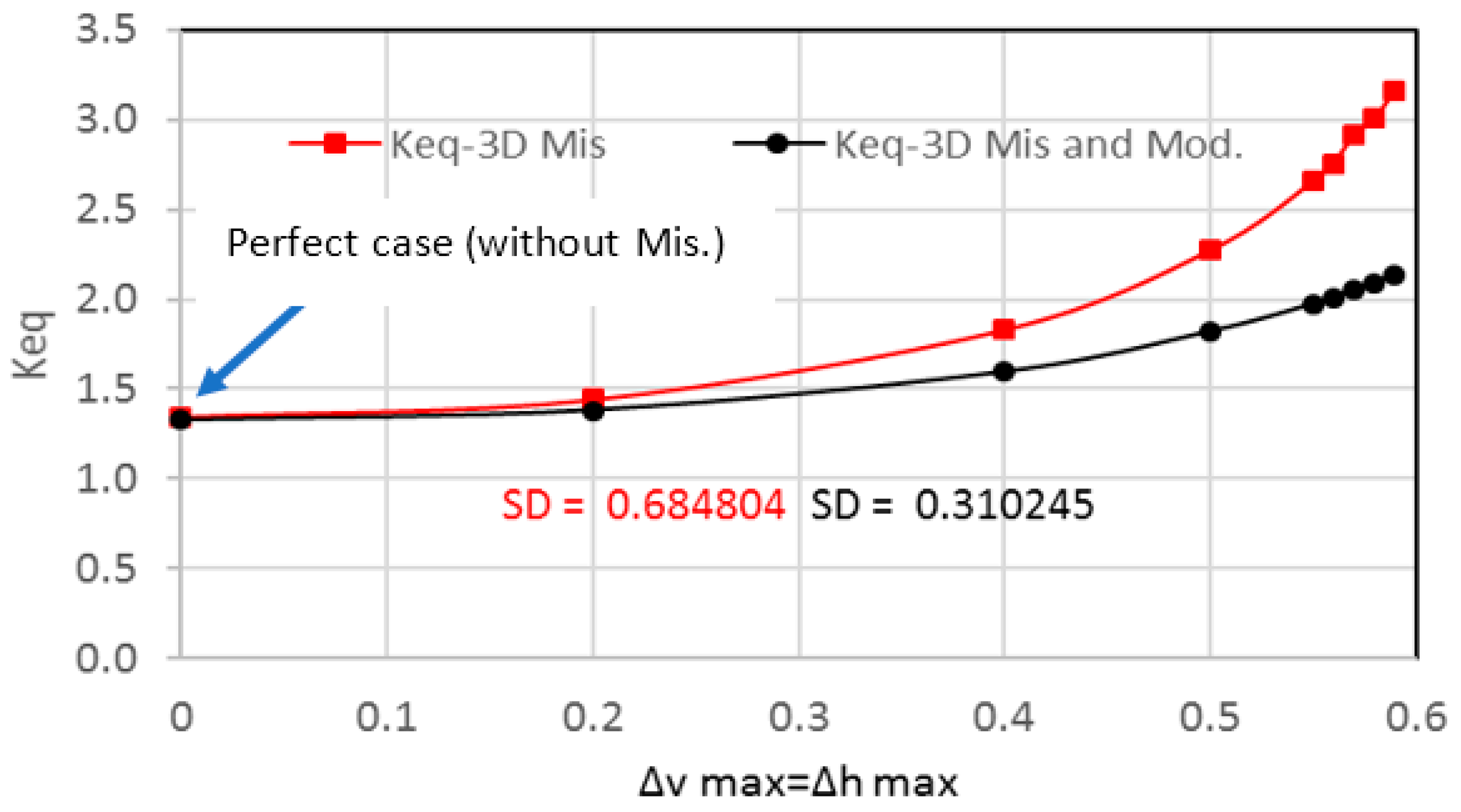
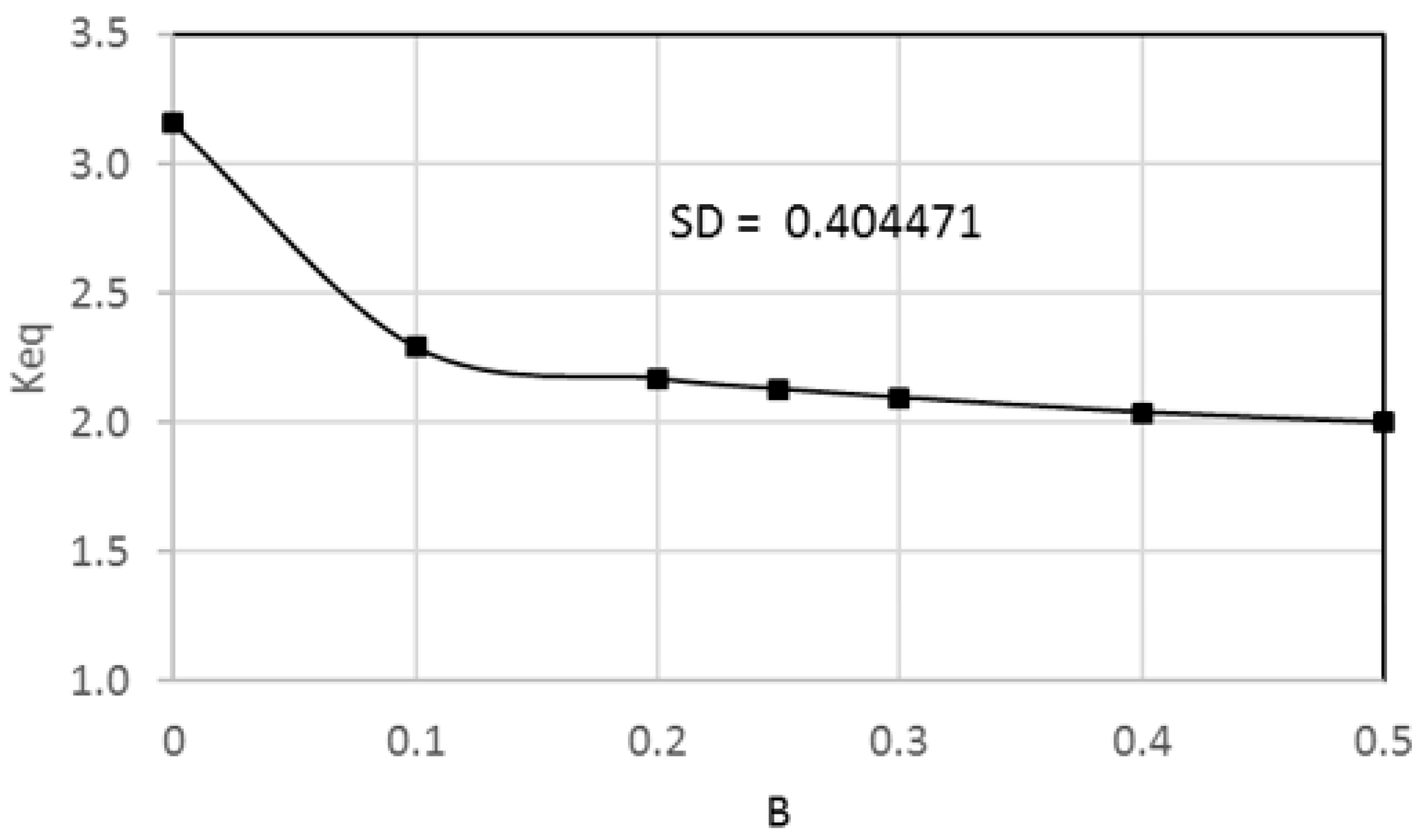
Figure 6 shows the variation of the equivalent stiffness coefficient for the modified and unmodified bearing geometry with a wide range of 3D misalignment parameters. Acceding this misalignment parameter range is insufficient for practical considerations as the minimum film thickness becomes extremely thin. It can be seen that for the ideal case (without misalignment) where
, the value of
is 1.347. As the misalignment parameters increase, the values of
also, increase with a maximum value of 3.161 when
. This increase means, in other words, an elevation in the level of the critical speed (which will be explained later) of the rotor bearing system, but large drawbacks accompany it in terms of H
min and P
max, as illustrated in the previous figure. Therefore, it cannot be considered an enhancement of the system’s performance. On the other hand, the geometrical modification of the profile reduces the
in comparison with the misalignment case. The reduction in
at the extreme case when
is 32.64% (
. Despite this reduction in
as a result of introducing the geometrical change in the bearing profile, the equivalent stiffness values for the whole considered range of misalignment parameters remain higher than the stiffness of the ideal case where
. The improvement in
for the cases of
is 58.1% in comparison with the ideal case. This outcome represents a significant improvement in the system performance due to the geometrical design changes, the previously mentioned reduction in P
max, and the significant increase in H
min. The modification parameters for the results presented in this figure are
. The effect of the design parameter
on the equivalent stiffness is shown in
Figure 7, and the optimum value of the other design parameter (parameter
) was found to be 0.25. It can be seen that increasing the length of modification along the axial direction of the bearing (parameter
) reduces the values of
. However, the equivalent stiffness coefficient is not continued to change significantly when
. This value of
also gives the best outcome in terms of Pmax and Hmin, which are therefore adopted for the main analysis in this work.
The effect of changing the geometry of the bearing on the dimensionless critical speed is shown in
Table 2. This table compares the critical speed for two levels of misalignment which are
and
in addition to the perfectly aligned case. The critical speed of the ideal case is 2.6789, and the misalignment increases the critical speed by 28.28% and 50.61% (3.4366 and 4.0347) for the misalignment’s first and last levels, respectively. Introducing the bearing profile modification reduces these values, but in all modified cases, the dimensionless critical speed is stills greater than the corresponding value of the unmodified ideal bearing. The dimensionless critical speed for the misaligned and modified case when
is 3.4121 compared with 2.6789 for the perfectly aligned case, representing an increase of 27.37%. This is another improvement in the dynamic performance of the rotor-bearing system.
After illustrating the importance of the bearing geometrical design on the key results related to the performance of the rotor-bearing system, the following results are related to the effect of unbalance excitations on the system’s dynamic behavior considering the bearing profile modification. Unbalance is a common machinery fault that results in due to the uneven distribution of a rotating component mass about its axis. Reference [
36] considered a dimensionless (scaled to the load) unbalance force
of 0.2, corresponding to an eccentricity ratio of 0.6 and a rotational speed of 3000 rpm (
. This means changing the rotational speed resulting in a different unbalance force. Therefore, the following factor,
is introduced to represent the unbalance force in terms of the rotational speed where
. Considering the value of 0.2 for
and
as used by reference [
36], results in a value of
for
. In this work, three values for
are considered in the analysis, which are
,
and
to evaluate the effect of unbalance excitation on the response of the system under different operating speeds. These values of
(
,
and
) mean that
and 0.3 respectively when
and give different values for
as
changes.
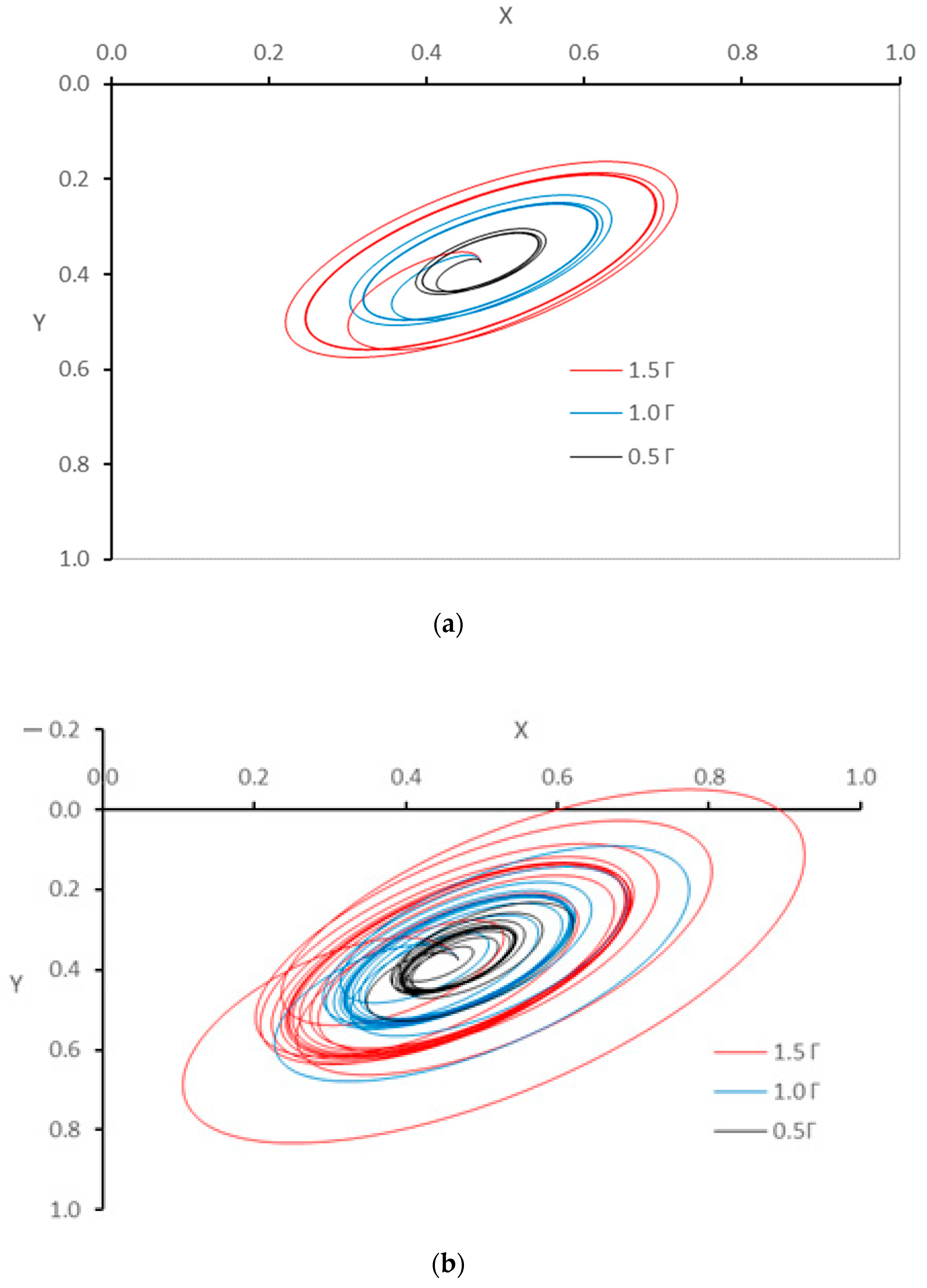
Figure 8 shows the trajectories of the journal center under different rotational speeds and unbalanced excitations (
,
and
) for unmodified bearing.
Figure 8a–c illustrate the trajectories when
which is about half the critical speed,
of the critical speed, and when
is equal to the critical speed, respectively. The dimensionless critical speed of the system is 2.6789 (6540.93 rpm). It can be seen that when
about half the critical speed of the system (
Figure 8a), the journal centers rotate about the steady-state position in almost the same path of rotation for each of the three values of
. The rotation amplitude increases as
increases, but in all cases, the trajectories do not cause the journal to be close to the bearing walls, and all the paths are uniform. As the rotational speed is increased, the trajectories follow different paths, as shown in
Figure 8b where
of the critical speed of the system. The higher value of
results in a non-safe trajectory of the journal center as the journal becomes very close to the bearing wall, and any error related to installation or the designed operating conditions may bring the surfaces of the shaft and the bearing much closer. This means in other words, that the presence of the unbalance forces in relatively high levels causes unsafe operation of the system despite that the operating speed is far from the value of the critical speed as shown in
Figure 8b where
of the critical speed.
Figure 8c illustrates the trajectories when the operating speed is equal to the critical speed. It can be seen that even for the lower value of
, the trajectory is not uniform, and the amplitude of rotation about the steady state position varies with time. This variation is increased as
increased as can be seen for the case of
shown in blue, and the amplitude of the rotation increased rapidly for the case of 1.5
where the journal touches the bearing walls.
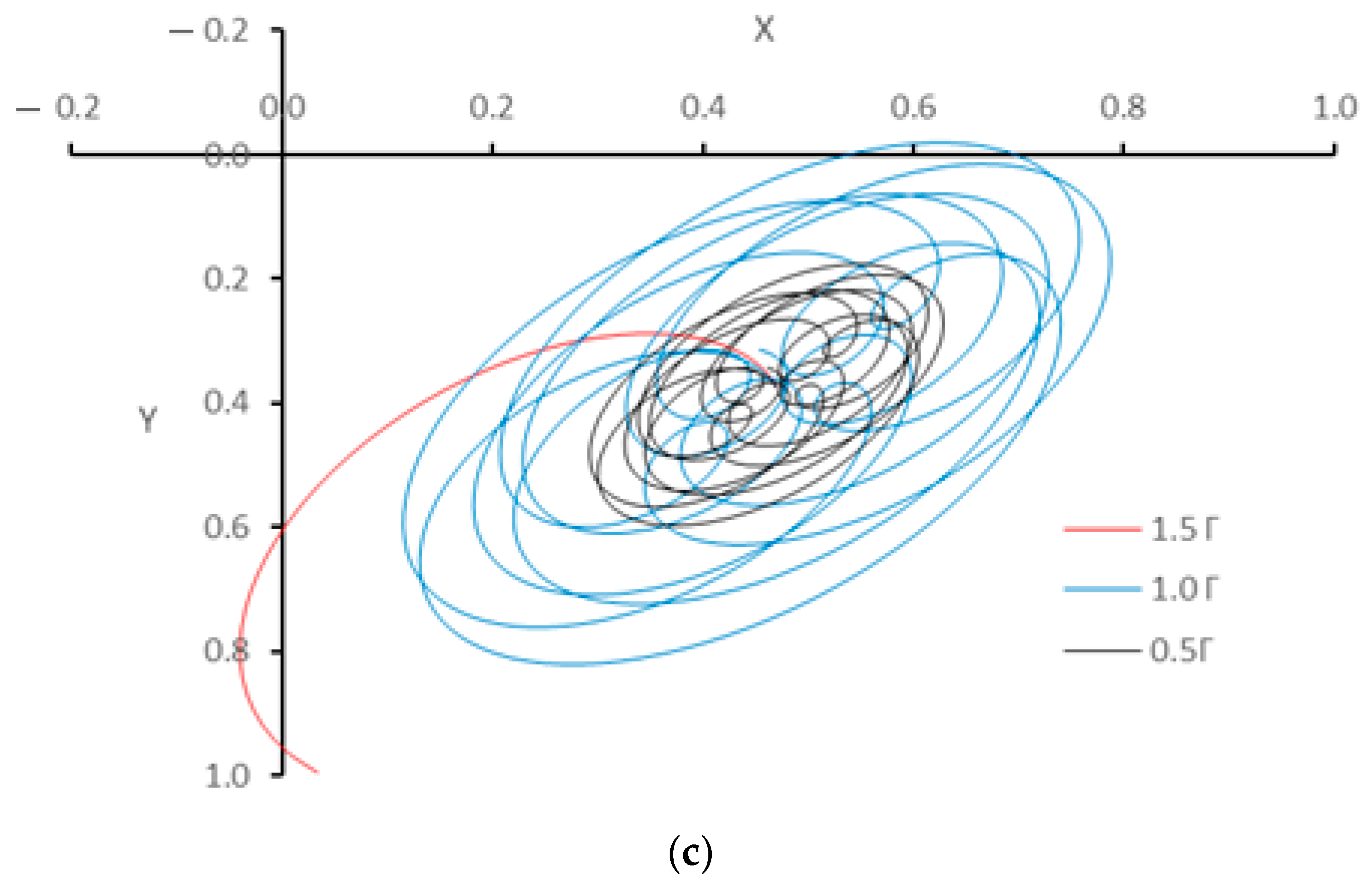
The trajectories of the journal center are further investigated by considering the bearing modification under an operating speed of 3000 rpm (
as shown in
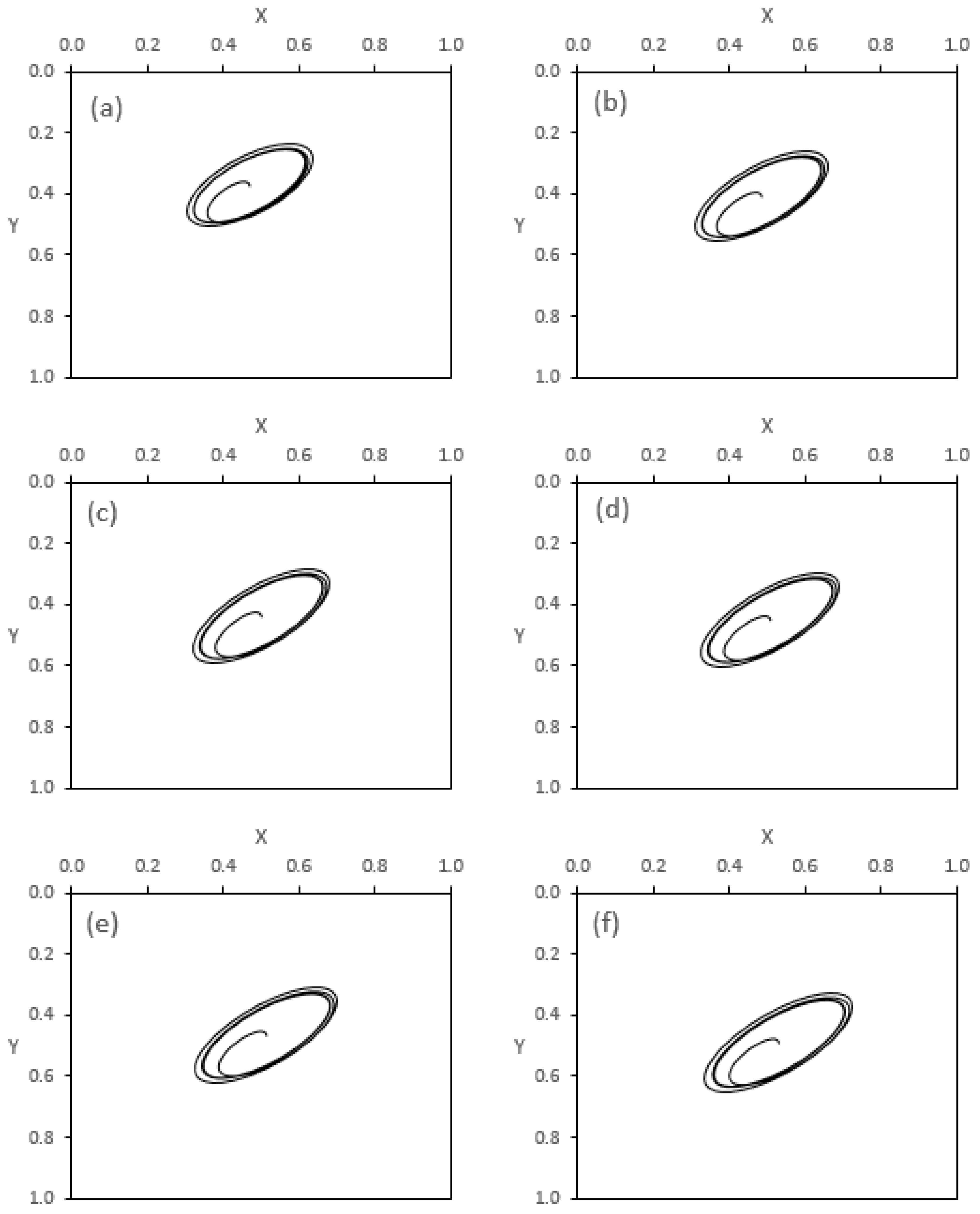
Figure 9. Different values of the geometrical parameters are considered in this figure.
Figure 9a shows the trajectory for the case of unmodified bearing, and the other figures illustrate the trajectories for the modified bearing where (
Figure 9b):
, (
Figure 9c):
, (
Figure 9d):
and (
Figure 9e):
. It can be seen for this operating speed, the trajectories are uniform for all values of the modification parameters, and the journal is far away from the bearing wall. This means that modifying the bearing geometry under
keeps the operation of the system in the safe range.
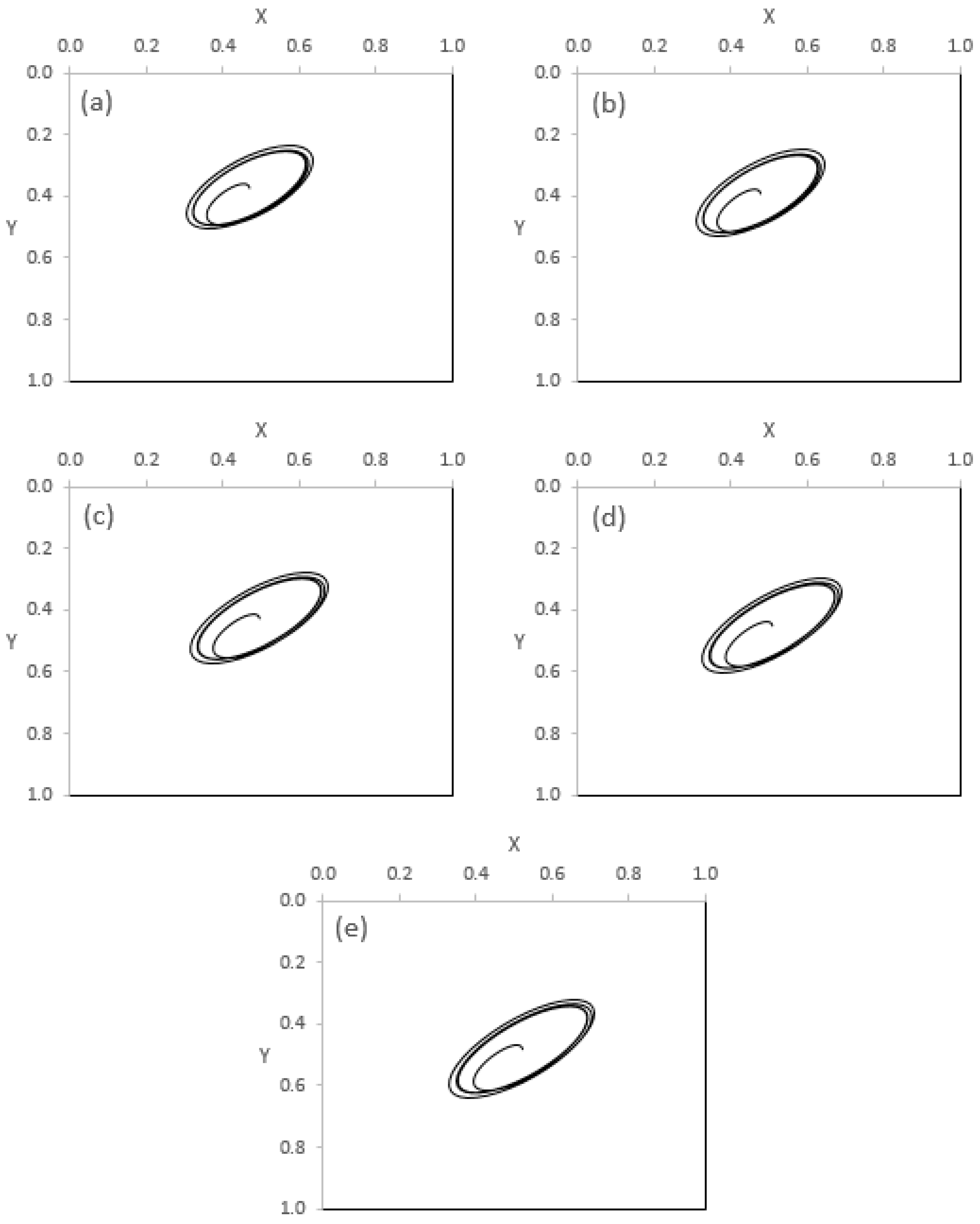
The effect of the modification parameter in the axial direction,
on the journal trajectory, is investigated for a constant value of the other modification parameter (
).
Figure 10 shows the results of these cases when the rotational speed is 3000 rpm (1.0
).
Figure 10a shows the case of the unmodified profile, which is repeated here from the previous figure for the purpose of comparison.
Figure 10b–f illustrate the trajectories for the cases when
,
,
and
. Again changing the
parameter also maintains the safe operation of the system under this operating speed.
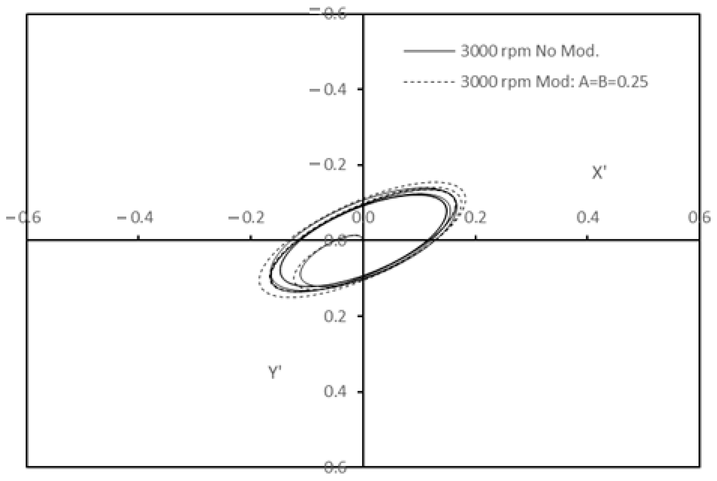
The previous figures show the trajectories relative to the bearing center using the
system of coordinates. To obtain a more clear comparison between the trajectories of the modified and unmodified system, the
,
system of coordinates is used in producing the results shown in
Figure 11. This figure illustrates the journal trajectories for the unmodified and modified bearing profile relative to the steady-state position (in terms of
and
coordinates) when the rotational speed is 3000 rpm (1.0
and
. It can be seen that the two trajectories are very similar, with a slightly higher amplitude of the rotation in the case of modified bearing. However, as illustrated in the previous two figures, the two trajectories keep the journal surface away from the bearing wall.
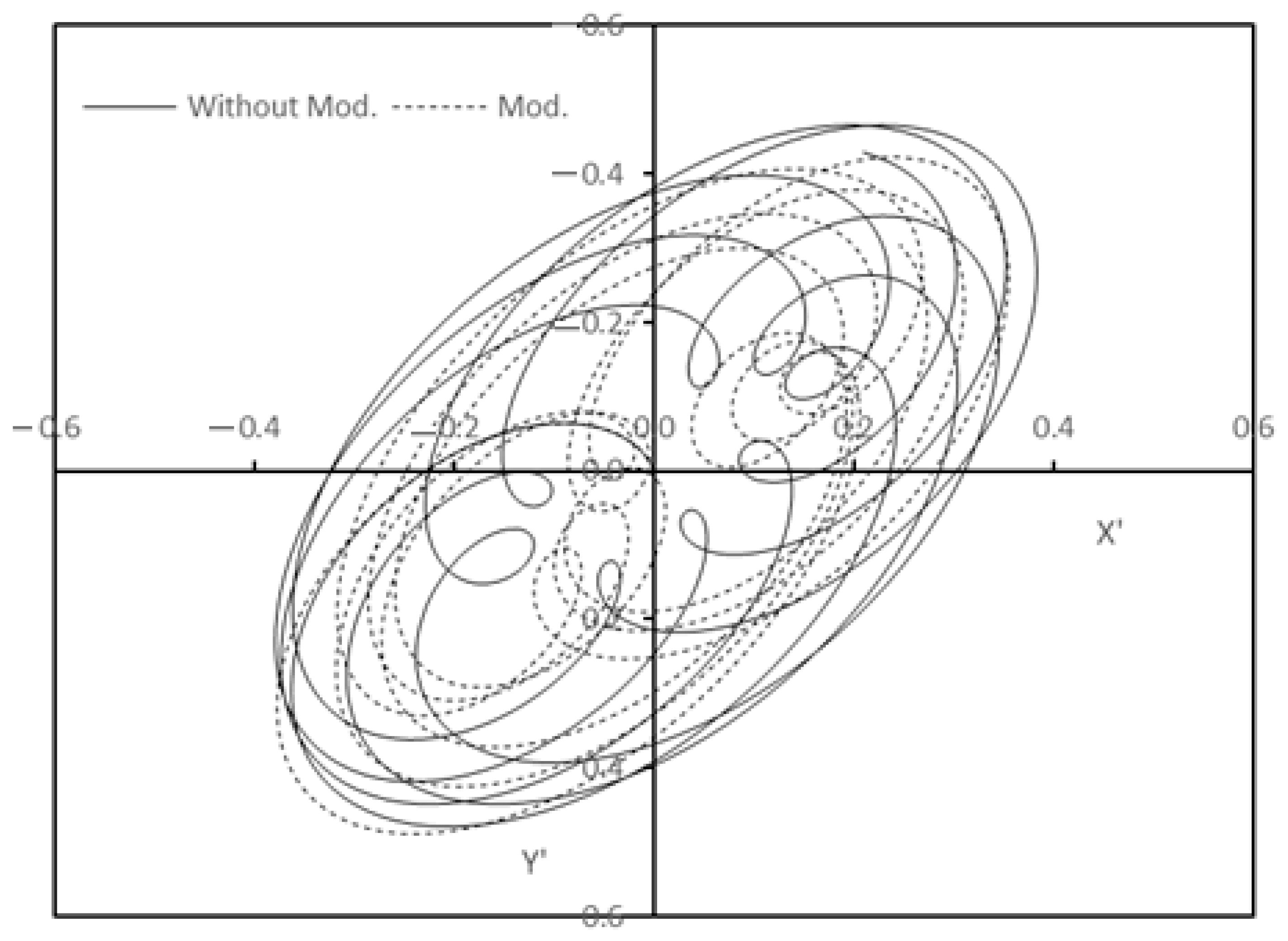
Figure 12 illustrates another comparison between the journal trajectories for the unmodified and modified bearing profile relative to the steady-state position (in terms of
and
coordinates) when the rotational speed is equal to the critical speed of the modified system, where the dimensionless critical speed is 2.8636 (6991.917 rpm) and the modification parameters are
. These results corresponding to the case when 1.0
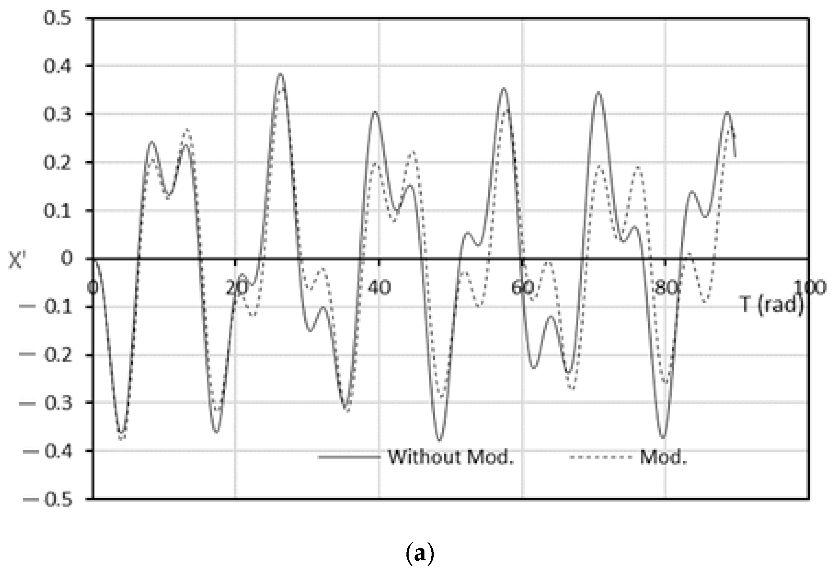
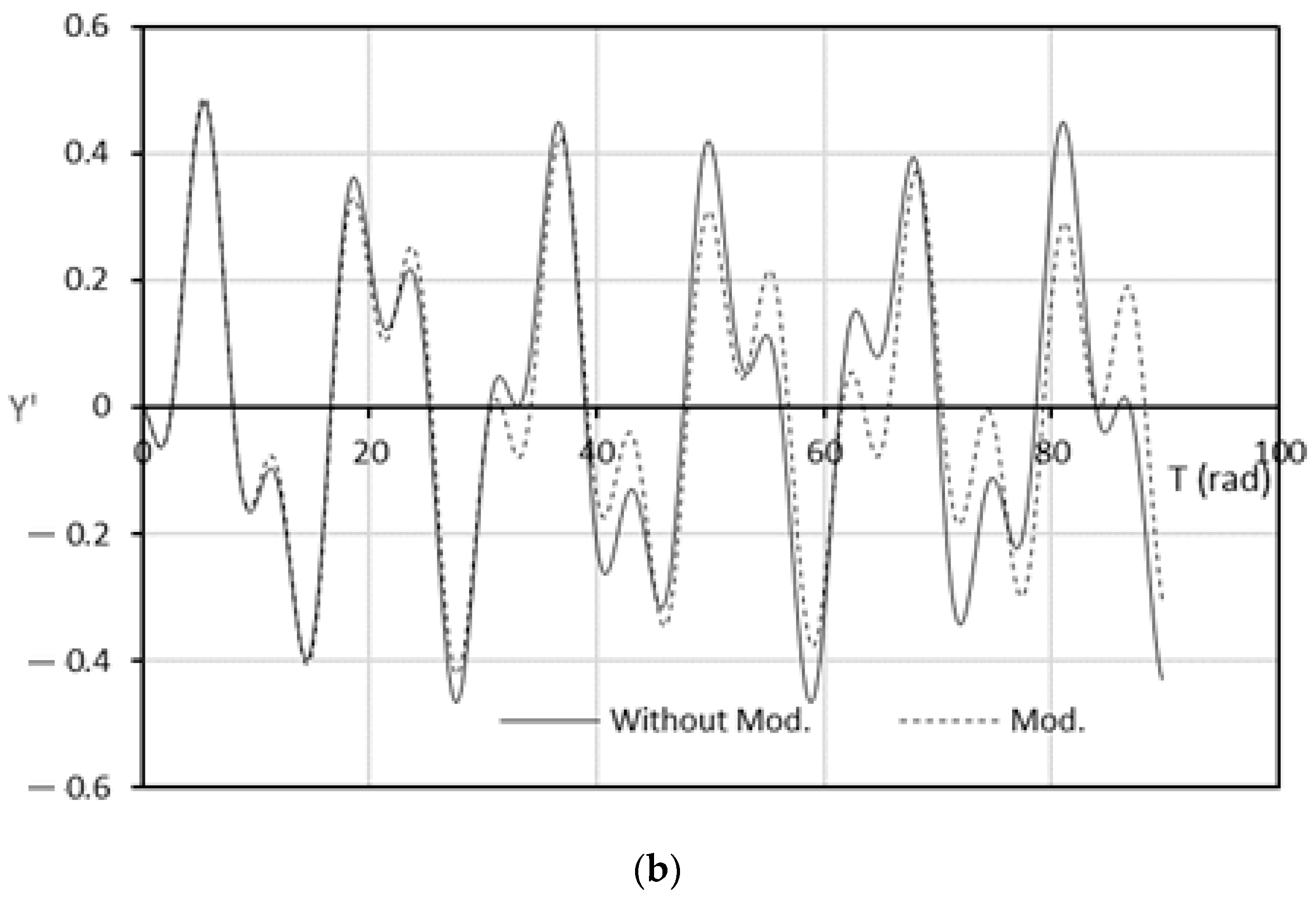
. Despite that both trajectories are non-uniform due to the relatively high operating speed, the journal, in the case of modified bearing, tends to rotate around the steady state position with less amplitude for most of the time. This difference can be seen clearly in
Figure 13, which illustrates the variation of
and
with the time
T (in rad) where
T = and the units of
and
t are rad/s and second, respectively. It can be seen that as
T increased, the values of
and
for the modified bearing are less than the corresponding values for the unmodified bearing for most of the duration of the response to the unbalance excitation.
It is clear from the above results that the modification helps in elevating the level of Hmin and reducing the levels of Pmax resulting from the 3D misalignment case and also resulting in higher critical speed in comparison with the ideally aligned bearing system. Furthermore, analyzing the system response under an unbalance excitation showed that the modification does not cause higher transient amplitude for the rotation around the steady state position at the high operating speed of rotation. This important outcome can be further advanced to consider the 3D misalignment in analyzing the response to unbalance excitation, which is an extremely complex case as the model requires a solution in space for the equations of motions. The authors intend to address this important issue in the near future work as both the misalignment and the unbalance excitation are common machinery problems.


 ,
, 


