Article

Solving Location Assignment and Order Picker-Routing Problems in Warehouse Management

by
Johanna Bolaños-Zuñiga
*,†,
M. Angélica Salazar-Aguilar
*,† and
Jania Astrid Saucedo-Martínez
*,†
Facultad de Ingeniería Mecánica Eléctrica, Universidad Autónoma de Nuevo León, Av. Universidad S/N, Ciudad Universitaria, San Nicolás de los Garza 66455, Nuevo León, Mexico
*
Authors to whom correspondence should be addressed.
These authors contributed equally to this work.
Axioms 2023, 12(7), 711; https://doi.org/10.3390/axioms12070711
Submission received: 29 May 2023 / Revised: 8 July 2023 / Accepted: 15 July 2023 / Published: 22 July 2023
(This article belongs to the Special Issue Applied Mathematical Modeling and Optimization)

Abstract

:
One of the critical warehousing processes is the order-picking process. This activity consists of retrieving items from their storage locations to fulfill the demand specified in the pick lists. Therefore, the storage location assignment affects the picking time and, consequently, reduces the operating costs of the warehouse. This work presents two alternative mixed-integer linear models and an adaptive multi-start heuristic (AMH) for solving the integrated storage location and picker-routing problem. The problem considers a warehouse with a general layout and precedence constraints for picking according to the products weight. Experimental work confirms the efficiency of the proposed reformulations since we found out a total of 334 tested instances and optimal solutions for 51 new cases and 62 new feasible solutions. The proposed AMH improved more than 29% of the best-known solutions and required an average execution time of 117 s. Consequently, our proposed algorithm is an attractive decision-making tool to achieve efficiency when solving practical situations in a warehouse.

1. Introduction

Companies need to perform supply chain management to satisfy customer demand and provide high-quality service. Therefore, all the involved activities must be aligned to this end, maintaining a balance between cost and efficiency. According to [1,2], warehouses are critical components of supply chains responsible for reception, warehousing, picking, packing, and shipping products between suppliers and customers. Hence, warehouse management is important for the proper operation of an organization, and any improvement that reduces costs will contribute to the efficiency and effectiveness of the supply chain.
Order picking is the highest-priority process in warehouses, representing around 60% of operational costs [3,4]. Hence, any performance improvement in this activity will allow us to reduce these costs. According to [5,6,7], one strategy to improve the order-picking process is to reduce the total picking time (or travel time) by simultaneously making decisions for the storage location assignment (tactical planning) and the picker-routing problem (operational planning). A correct product location facilitates and accelerates the retrieval of orders and improves the productivity of other warehouse activities [8], allowing better customer service.
Although much of the research focuses on studying both decisions independently, based on the literature [9,10], optimizing each problem separately may lead to a suboptimal solution for the entire warehouse. Since new trends in the logistics industry require even more efficient picking operations, these problems must be considered simultaneously to be competitive in the market.
According to [11], even though studying both problems simultaneously is not new, some researchers oppose this method and believe that the integrated model can be useless due to the different time horizons of both problems since the routing is an operational problem with short time horizons while the storage location has a more extended period. Nevertheless, in [12], the simultaneous method presented better results than the independent method. In the same way, authors from [11] mentioned that integrating storage location and picker-routing decisions is a well-practice that has demonstrated its advantages to improve picking efficiency, mainly when the demand of each product and the products contained in each order are known.
Significant efforts have been made throughout the past 30 years to improve the order-picking process [4,13]. Based on [14,15,16,17], the weight of the products is a barely considered feature, which may be a key consideration when retrieving the products from the orders since it avoids impacts or damages on the items. The main motivation to consider the weight of the products is that planning the retrieval routes of the orders does not consider this factor. Consequently, pickers choose alternative routes to keep a good presentation of the final product (customer order). However, this deviation from the planning routes carries out an increment in the picking times. Therefore, the company employs additional labor to deliver customer orders at the right time and in the right condition. See Section 3 for more details about the case study.
In this work, we integrate storage location and picker-routing decisions with precedence constraints (according to the weight of the products) to solve a warehouse management problem recently introduced by [18]. The aim is to propose new mathematical reformulations by adding valid inequalities and sub-tour elimination constraints based on the flow of a single commodity proposed by [19] to improve the computational performance of the existing optimization model proposed by [18]. Similarly, we propose a heuristic that can generate high-quality solutions (close to optimal) for all instances tested.
The next part of this work is structured as follows: Section 2 provides a brief review of the related work. Section 3 presents a general description of the case study. Section 4 describes the proposed reformulations and the adaptive multi-start heuristics. Section 5 shows experimental results and discussion regarding the performance of the proposed models and algorithm. Finally, Section 6 presents our conclusions.

2. Related Work

In the literature [9], three main problems were established: the planning of customer orders, batching, storage location assignment, and order picker routing. They mentioned that the storage location and routing are among the top-performing excellent planning problem combinations to minimize the picking time. However, even though several authors have widely studied these problems in the literature, such as [5,6,7,14,20,21], most of their methodologies focus on developing solution methods in the warehouse with rectangular or block layouts. Nevertheless, other non-traditional layouts exist, such as the fishbone used in [22,23,24], U-shape in [25], an unusual layout presented in [17], an irregular layout used in [26], a layout of the robotic mobile fulfillment system (RMFS) in [27,28], or the general warehouse studied by [18], which is used in this work. On the other hand, although our case study company does not use a radio-frequency identification system (RFID), in the literature [29], the authors developed an interesting contribution for the optimized RFID system for different warehouses with an L-shape and U-shape. Additionally, they mentioned the importance of studying other warehouse shapes rather than the rectangular shape.
To determine the total picking time, [1] identified four main activities, setup, searching, picking, and travel, where travel is the most expensive activity (representing 55% of the picking time). Furthermore, based on [3], travel represents the only variable part since it depends on the total length of the picker routing [30], while the other activities can be taken as constants.
According to [9,30,31,32], the picker-routing problem belongs to the NP-Hard class of issues since it can be interpreted as a special case of the traveling salesman problem (TSP) or the vehicle routing problem (VRP), depending on the features of the problem. Hence, solving the storage location and the picker-routing problem could be very difficult. Therefore, exact methods [30,33], heuristics [14,20,22,34,35], metaheuristics [5,11,16], genetic algorithms [7,36], and stochastic models [24,28] have been proposed to solve both problems sequentially or integrated.
Some related work to integrating location assignment and order picker-routing decisions can be found in [5,7,11,18]. In the literature [5], although the authors proposed a mathematical model and a metaheuristic algorithm, they did not consider the weight of the products in the routing, and a single product was assigned to multiple locations within the warehouse. However, in [7], the authors did not consider the criterion of the weight of the products when assigning them to the locations. For the routing, they contemplated the concept of the shortest order-picking routes in the proposed genetic algorithms. On the other hand, in the literature [11], although the authors presented different non-linear models, their respective linearizations, and a GNV metaheuristic, the authors did not consider the weight of the products in the routing policies used. Finally, in [18], even though the authors proposed a mathematical model, where precedence constraints were considered based on the weight of the products in the routing and a unique location for each product in a warehouse with a general design, it was not possible to find the optimal solutions for all the analyzed instances, leaving the way for the proposal of more efficient algorithms to address this issue. Therefore, since this last work deals with the characteristics of the case study, the mathematical model called SLAUPR by the authors is used as a framework in the present research. See Section 4.1 for more details about the SLAUPR model. Table 1 depicts an overview of works related to combining the storage location assignment problem and picker-routing problem.
It is noteworthy that factors such as inventory level, uncertain demand, or product deterioration are criteria that affect storage policies. See, for instance, Refs. [37,38], where the authors studied the topic of strategic planning in a multi-period multi-product inventory model under uncertain demand to minimize the storage locations and developed inventory models with conditions of deterioration of products, respectively. However, in this work, these criteria are omitted, given the characteristics of our case study.
Table 1. Overview of works related to combining the storage location assignment problem and picker-routing problem.
WorksPicking SystemWarehouse LayoutIntegrated SolutionStored in Multiple LocationsConsidered FactorsMethod
Daniels et al. [5]Low-level-DemandMathematical model. Metaheuristic (Tabu search)
Dekker et al. [14]Low-levelMultiple blocksXXDemand. Type of productHeuristics
Dijkstra and Roodbergen [21]Low-levelSingle blockXXDemandDynamic programming
Žulj et al. [15]Low-levelSingle blockXXWeight of productExact algorithm
Bolaños-Zuñiga et al. [18]Low-levelGeneralXDemand. Weight of productMathematical model
Kordos et al. [7]--XDemandGenetic algorithms
Silva et al. [11]-Single blockXDemandMathematical model. Metaheuristic (GVNS)
Cai et al. [27]RobotRMFSXDemandMathematical model
Keung et al. [28]RobotRMFSXXDemandDeterministic and stochastic models. Shortest path heuristics
Xu and Ren [35]Low-levelSingle blockDemand correlations. Congestion of pickersMathematical model. Heuristic
Zhou et al. [24]Low-levelFishboneXXDemandStochastic model
Lee [39]Low-levelSingle and two blocksXFrequency and relation of SKUsAnalytical models
Alqahtani [40]High-level-XXPicking frequencyAnalytical formulas
This workLow-levelGeneralXDemand. Frequency and weight of productMathematical model. Heuristic
Although several heuristics or algorithms have been proposed to simultaneously or sequentially solve the above-referenced problem with different variants (as seen in [41,42,43]), as far as we know, no other work in the literature has improved the results reported by [18]. However, when we try to solve the problem with a commercial solver like CPLEX, it struggles to find even feasible solutions when the instance size is medium or large.
Therefore, to improve the computational performance of the SLAUPR, the main contribution of this research is the development of mathematical reformulations considering valid inequalities and single commodity flow constraints for sub-tours elimination, as well as the design of an adaptive multi-start heuristic (AMH) as an approximation method to solve real-size or large instances in a short computation time. The AMH is a relatively simple heuristic based on articles such as [44,45,46]. It consists of two main phases, construction and improvement, which require few parameters to be tuned, and it performs well on many combinatorial optimization problems [47,48].

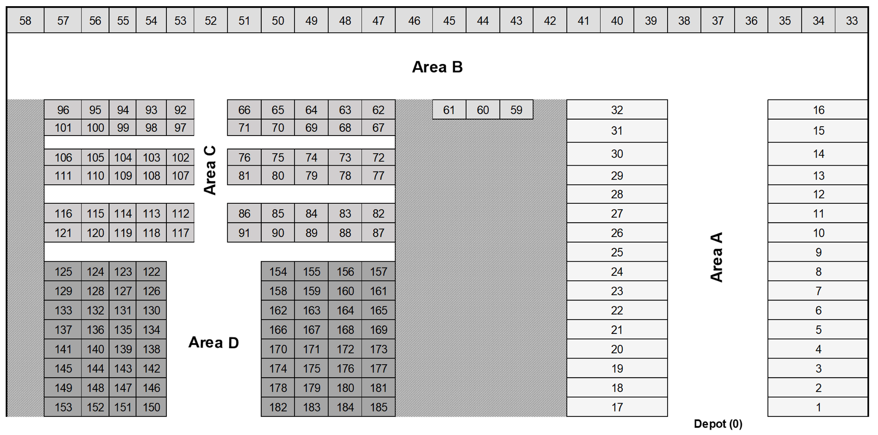
3. Case Study Description

The proposed method is motivated by a situation presented in the warehouse of products sent abroad (called exportation warehouse) of a company in the food sector located in Monterrey, Mexico. The company is well known for its excellent delivery service and presentation of customer orders, and keeping this standard is very important. The company owns the production and supply echelons of its supply chain. Thus, in this work, we do not consider a transportation disruption that occurs within the transportation. Nevertheless, in practice, there are some companies whose suppliers and transportation belong to different companies, and there are risks in the transport and manufacturing of products. See, for instance, Ref. [49], where the authors proposed some strategies to address the transportation hazard problem.
The company has a warehouse with a general layout (see Figure 1) and stable product demand per period, mainly dependent on the seasons of the year. For that reason, the storage locations of products may change periodically. The warehouse has 185 available storage locations divided into four areas (A, B, C, and D). Each stock-keeping unit (SKU) is based on its request frequency (the request frequency of a product is the number of times the product is demanded during a specific period.) or demand and assigned to a unique storage location within a specific area. Each SKU represents a box with the same type of product (i.e., cookies and bread). The SKUs in areas A, B, and C are stored on pallets, and in area D, the product is stored in boxes. The company does not have any issue to fulfill the demand, but the storage locations in the warehouse have different physical capacities. These capacities are sufficient to satisfy the demand for any product and are known in terms of boxes, contingent upon the type of product assigned.
In the studied problem, warehouse management is performed through a warehouse management system (WMS). The system generates the route or sequence that the picker must follow through the warehouse to retrieve the requested product (low-level picking). However, when planning these routes, which must start and end at the depot, the system does not consider the weight of the SKUs boxes (even though it is known), so pickers choose alternate routes to keep a good presentation of the customer orders. Usually, these decisions increase the picking time since the products do not have an appropriate storage location.
Consequently, the company allows extra labor hours to keep customer satisfaction, representing more cost and decreasing productivity. Based on [50], minimizing travel time is essential in reducing costs and delays. The research of [18] proposed a mathematical model to solve the increase in picking time problem. However, due to the complexity of the problem, for some real-size instances, there is no known feasible solution. Therefore, in this research, we propose new models and a heuristic to improve the best-known solutions and to have a decision-support algorithm that can be used in practice.

4. Materials and Methods

Due to the low performance achieved with the SLAUPR proposed by [18], it is hard to solve instances with medium and large sizes. Therefore, we propose two reformulations for the SLAUPR (see Section 4.1) and an adaptive multi-start heuristic (see Section 4.2). Table 2 provides the notation employed in the mathematical models and the proposed heuristic.

4.1. Proposed Reformulations

First, we describe the formulation introduced by [18] (SLAUPR), followed by the proposed reformulations. For the first reformulation, we propose valid inequalities for the SLAUPR model and better bounds for some constraints. We propose another formulation for the sub-tour elimination constraints for the second reformulation.
The SLAUPR formulation is the following:
m i n i I j I p P t i j u p i j
s . t : j I v p j k d k p k X , p P
p P v p j k Q j k j I , k X
j I { 0 } u p 0 j = 1 p P
k X e j k 1 j I
j I { 0 } e j k = 1 k X
v p j k M p j k i I u p i j k X , p P , j I
v p j k M p j k e j k k X , p P , j I
j I u p i j 1 i I , p P , i j
j I u p j i 1 i I , p P , i j
s i p s j p + | I | u p i j | I | 1 i , j I { 0 } , p P , i j
u p i i = 0 i I , p P
i I u p i j = i I u p j i j I , p P , i j
k X e i k w k l X e j l w l M ( u p i j 1 ) i , j I { 0 } , p P
u p i j { 0 , 1 } i , j I , p P
e j k { 0 , 1 } j I , k X
s j p 0 j I , p P
v p j k Z 0 + p P , j I , k X .
The objective function (1) minimizes the travel time. Constraints (2) and (3) guarantee the satisfaction of the demand and the capacity of the storage locations, respectively. Condition (4) defines the depot as the beginning point for each route. Constraints (5) and (6) assign each product to a unique storage location, but not all locations need to be allocated. Constraints (7) and (8) link the retrieved products to the assignment and routing variables. Constraints (9) and (10) guarantee that each location is visited at most once on each route. Conditions (11) and (12) correspond to the sub-tours elimination constraints (MTZ) proposed by [51]. These sets of constraints are needed since some products have the same weight. Constraint (13) guarantees the flow conservation by order. Precedence constraints based on the weight of the products (14). Finally, Constraints (15)–(18) correspond to the variables domain. However, the main difficulty presented by SLAUPR is that when a general-purpose solver tries to solve the problem using this model, it struggles to find even feasible solutions.
Then, with the aim of strengthening the SLAUPR performance, we analyzed the existing formulation, derived valid inequalities, and reformulated the sub-tour elimination constraints as follows:
  • Constraints (3) and (8) were merged since it is possible to guarantee with a single constraint that the product is retrieved without exceeding the capacity (inventory) of the corresponding storage location:
    p P v p j k Q j k e j k j I , k X .
  • Redundant constraints (10) were removed.
  • Constraints (11) were replaced by
    s i p s j p + ( M p + 1 ) u p i j M p i , j I { 0 } , p P , i j ,
    where M p corresponds to the number of different products in order p P . M p is a new parameter that is created to bound | I | without losing feasibility in Constraints (11).
  • In Constraint (14), parameter M is set as M = max k X { w k } to bound the value in this parameter.
Considering the previous modifications, the first proposed reformulation, referred to as SLAUPR_V2, is composed of expressions (1), (2), (4)–(7), (9), (12)–(18), (19), and (20). Therefore, SLAUPR_V2 has two fewer sets of constraints than the SLAUPR.
Based on the empirical results from literature [52], the elimination of sub-tours proposed by [19] presents better performance than other analyzed formulations. Therefore, according to the structure of the SLAUPR, it is proposed to replace Constraint (20) and perform a reformulation using constraints presented by [19]. Variables g p i j are added to describe the flow between location i I and j I in each order p P . The proposed sub-tour elimination constraints are the following:
g p i j M p u p i j i , j I , p P , j 0 ,
j I g p j i j I { 0 } g p i j = j I { 0 } u p j i i I { 0 } , p P .
Constraints (21) guarantee the flow corresponding to the number of products to be retrieved, and constraints (22) ensure that in each location included in the route, a single unit of the flow is left.
Based on the above, the second mathematical reformulation proposed, which we named SLAUPR_V3, is composed of expressions (1), (2), (4)–(7), (9), (12)–(18), (19), (21) and (22). Hence, the proposed model SLAUPR_V3 has one fewer set of constraints than the SLAUPR but one more than the SLAUPR_V2.

4.2. Proposed Heuristic

It is well known in the literature that using heuristics or metaheuristics can accelerate the convergence of exact methods and provide a favorable time solution to complex or real-size problems. Therefore, due to the complexity of the SLAUPR, we also designed an adaptive multi-start heuristic (AMH) based on the greedy randomized adaptive search procedure (GRASP). One of the main advantages is the ease of implementation and the construction of high-quality solutions that are later improved, usually with a local search procedure that starts from the constructed solution by exploring a defined neighborhood iteratively. Also, the AMH has been plenty employed due to its efficiency in sorting out complex vehicle routing problems as mentioned in the works of [53,54,55].
We focused on the design of each AMH phase to generate high-quality solutions in a short computational time. Furthermore, to restrict the candidate lists (RCL), in the constructive phase, the value of the quality parameter ( α ) is automatically tuned during the solution process, depending on the instance on hand.
A general scheme of the proposed AMH can be seen in Algorithm 1. Let iter _ 1 be the maximum number of iterations of the constructive improvement cycle; instance is the instance on hand; α { 0 , 1 } is a quality parameter; f(S) represents the objective function value or total picking time; and lsIter and lsTime are the consecutive non-improvement solutions and the execution time limit for the improvement phase, respectively.
Algorithm 1 Adaptive multi-start heuristic (AMH).
  • Input: instance, iter _ 1 , lsTime, lsIter  α
  • Output:  S * : the best solution found
1:
for  i = 0   to  Iter _ 1   do
2:
     S  Constructive phase(instance, α )
3:
     S * S
4:
     c o u n t e r 0
5:
    while  t i m e  lsTime &  c o u n t e r  lsIter do
6:
         S Improvement phase ( S * , lsIter, lsTime)
7:
        if f( S * ) > f( S ) then
8:
            S * S
9:
            c o u n t e r 0
10:
        else
11:
            c o u n t e r c o u n t e r + 1
12:
        end if
13:
    end while
14:
     i i + 1
15:
end for

4.2.1. Constructive Phase

The proposed algorithm for the constructive phase consists of a randomized construction heuristic (RCH) composed of two steps: the first one is related to the storage location assignment, and the second one to the sequence of order retrieval and total picking time by considering the constraints of the problem. Algorithm 2 depicts the procedure for the first step.
A candidate list (CL) is generated with the evaluation function values, denoted as fa [ k ] , of each product k X to determine the first product that will be assigned. Subsequently, a restricted candidate list (RCL) is created. The elements to include are determined by CL [ k ] { CL m i n , CL m i n + α ( CL m a x CL m i n ) } , where α is a quality parameter, and CL m i n and CL m a x are the minimum and maximum values of the CL, respectively.
Notice that if α = 0 , the RCL only contains the CL m i n element. While if α = 1 , the RCL will include all the elements of the CL, which implies that the final solution could be completely random. So, the α value helps to restrict the selection of the best elements during the construction of the solutions.
The evaluation function used in our AMH is defined by Equation (23):
fa [ k ] = w k f p k ,
where f p k is the request frequency of the product k X , i.e., the number of pick lists where product k X is demanded.
Once the elements in the RCL are determined, one product is randomly chosen and removed from the CL. To decide the storage location j, we use the nearest neighbor criterion; based on t i j , we calculate timeNeighbor [ i , j , 0 ] i I , j I { 0 } , which is the traveling time from location i I to location j I { 0 } and returning to location 0, defined as the starting and ending location (depot). Hence, the best storage location to assign the first product will be the one with the smallest value of timeNeighbor [ 0 , j , 0 ] , where j I { 0 } is the nearest free adjacent location to location 0.
For the next product to be assigned, the RCL starts over. One product is randomly chosen and removed from the CL. To decide the location assignment, a free adjacent location to the last assigned location i I is the one with the smallest value of timeNeighbor [ i , j , 0 ] . In the event of a timeNeighbor [ i , j , 0 ] tie between several free adjacent locations, one of them is randomly chosen. The previous process is repeated until all the products k X are assigned to a unique storage location j I { 0 } , where assignProductToLocation represents the relation of products to storage locations.
Algorithm 2 First step of the RCH: storage location assignment.
  • Input: Instance, α .
  • Output:  assignProductToLocation
1:
Compute fa [ k ] k X
2:
Generate CL
3:
Calculate timeNeighbor [ i , j , 0 ] i I , j I { 0 }
4:
l 0
5:
while  CL   do
6:
    Create RCL  { r C L , r C L m i n + α ( C L m a x C L m i n ) }
7:
    Randomly choose r *
8:
    Remove r * from CL
9:
     j arg min l I { 0 } timeNeighbor [ l , j , 0 ]
10:
    assignProductToLocation( r * , j * )
11:
     l j *
12:
end while
After assigning products to storage locations, the second step of the RCH consists of determining the routes the picker must follow to retrieve the products from each order. The products from each order are collected by following a decreasing arrangement of the weight of the products. Finally, f(S) is the resulting sum of the picking time of the generated routes.

4.2.2. Improvement Phase

The proposed improvement phase is a local search procedure, in which an initial solution is obtained from the RCH. The neighborhood is explored based on the first improvement, which moves to the first feasible solution that improves the value of the current solution.
For building the neighborhood, we propose a strategy that switches the storage location of a pair of products with similar weights to minimize the total picking time. To determine which products k 1 and k 2 are exchanged, the first one, k 1 , is randomly chosen. Subsequently, a product k 2 of equal or similar weight is identified, and storage locations are exchanged. AMH stops when it reaches a maximum number of iterations (lsIter = 200) or a maximum time limit (lsTime = 60 s). The process is repeated until a stopping criterion is met, and the best-found solution is reported.
The lsIter and lsTime values are determined based on the results of a design of experiments. For lsIter, the heuristic shows that after 200 iterations, the value of the solution found by the local search does not improve. For lsTime, it shows that for the local search, the execution time of each analyzed instance is less than 60 s.

4.2.3. Adaptive Process

To avoid the manual calibration of the quality parameter α used to create the RCL, the value of this parameter is automatically tuned according to the results in the previous iterations. Therefore, the parameter α can take any value from a discrete set Λ = { α 1 , α 2 , , α m } of possible values with a probability of p i . Then, in the first iteration of the AMH, each value has the same probability of being selected p i = 1 m , i = 1 , 2 , m .
According to [48,56], after a definite number of iterations, the probabilities for each α are periodically recomputed using Equation (24):
p i = q i j = 1 m q j ,
where q i = 1 A i , and A i represents the average objective value of all solutions found by using α i Λ . According to the definition of q i , it can be deduced that if the selected α m has found good solutions, then its p m will be higher.
Let Iter _ 2 be the number of iterations to recompute the probabilities p i . Matching some of the most commonly used methodologies in the literature and a design of experiments, ten possible values for α are utilized for the AMH and the value of Iter _ 2 = 100 .

5. Results and Discussion

The performance of our proposed solution methods are evaluated in the instances presented by [18]. The instances are categorized into four scenarios and four different sizes. The main characteristics of the instances are displayed in Table 3. Column Storage location ( | I | ) represents the number of available storage locations. Column Requested products shows the range of the total number of the requested products. Column Products to assign ( | X | ) displays the range of the number of different products to be assigned. Column Order to pick ( | P | ) shows the number of requested orders. Finally, Column Number of instances represents the number of instances available in the literature. See [18] for more details.
The proposed SLAUPR_V2 and SLAUPR_V3 were developed in GAMS software version 23.7.0 Cplex 12. We considered the same stopping time proposed by [18]: 3600 s for instances of up to 32 locations, 7200 s with 61 locations, 10,800 s with 121 locations, and 14,400 s for instances with the 185 locations available in the warehouse.
The proposed AMH was coded in C++, the maximum number of iterations was set to 1000, and the set of values of the quality parameter α was defined as Λ = { 0.1 , 0.2 , 0.3 , 0.4 , 0.5 , 0.6 , 0.7 , 0.8 , 0.9 , 1.0 } .
The experiments were carried out on a computer with a 2.4 GHz Intel Xenon processor, 64 GB RAM, and a hard disk with a 2 TB capacity.

5.1. Proposed Reformulations

Table 4 shows a summary of the obtained results. The F/O columns describe the number of solutions and the number of optimal ones reported in the literature (SLAPR) and found with SLAUPR_V2 and SLAUPR_V3, respectively. The Average optimality gap (%) columns represent the average percentage of the optimality gap reported by CPLEX of each method.
According to the results shown in [18], for the small and medium type_1 instances, scenario_1 and scenario_2 are the least complex. In contrast, scenario_3 and scenario_4 are the ones that present the highest complexity, except when only one order must be picked. Moreover, all scenarios are complex for the medium type_2 and large instances to be optimally solved. Therefore, [18] does not report feasible solutions from scenario_4 of medium type_2 and scenario_1 of the large size.
Table 4 shows that the solutions found by the proposed SLAUPR_V2 and SLAUPR_V3 are competitive compared to the results by SLAUPR. Notice that for small instances, both proposed models find six new cases with optimal solutions for scenario_3 and scenario_4, respectively. However, the average optimality gap obtained by the SLAUPR_V3 model for the instances of these scenarios (3.83% and 8.48%, respectively) is better than that reached by SLAUPR_V2 (19.24% and 23.27%, respectively), as well as for those reported in the literature (33.47% and 35.92%, respectively).
For medium type_1 instances, both models find better results than those reported in the literature. SLAUPR_V2 obtains 12 new cases with a feasible solution and 27 with an optimal solution, while SLAUPR_V3 finds 33 new cases with a feasible solution and 29 with an optimal solution. Similarly, the average optimality gap achieved by the SLAUPR_V3 model for the instances of the four scenarios (6.15%, 15.63%, 23.54%, and 54.98%, respectively) is better than the average achieved by SLAUPR_V2 (7.68%, 13.13%, 15.20%, and 74.43%, respectively), as well as for those reported in the literature (32.11%, 22.62%, 14.21%, and 63.49%, respectively). In scenario_3, it is observed that SLAUPR_V3 reports a higher average value of the optimality gap since this model achieves finding ten new cases with a feasible solution, more than those found with SLAUPR_V2 and those reported in the literature. It should be noted that, for this scenario, the instances where the optimum is reported and found are those where only one order is requested. However, in scenario_4, despite the SLAUPR_V3 finding a more significant number of new cases with a feasible solution, the average optimality gap is better than SLAUPR_V2 and that reported in the literature since the minimum and maximum optimality gaps reached by both models are greater.
For medium type_2 instances, although the SLAUPR_V2 model presents better performance for scenario_3 since it manages to find a greater number of new cases with an optimal solution and the lowest average optimality gap (22.44%) of the three models, the SLAUPR_V3 model, in general, finds ten new cases with a feasible solution and two with an optimal solution, with the main contribution being able to obtain a case in scenario_4 with a feasible solution.
For large instances, SLAUPR seems to have the best average results; however, in scenario_2, the SLAUPR_V2 model reports three new feasible solutions. In scenario_3, the SLAUPR_V3 model finds feasible solutions to two new cases. Nevertheless, a feasible solution to the instance based on real data is still not found with any of the reformulations, and feasible solutions continue with an optimality gap greater than 80%.
Finally, another essential aspect to highlight from the results by the proposed SLAUPR_V2 and SLAUPR_V3 models is the execution time compared to the one reported by the SLAUPR since for the 90 instances analyzed in the small size and the 144 in the medium type_1 size, the SLAUPR_V3 model reduced the execution time, on average, by 48.47% and 22.34%, respectively. In contrast, the SLAUPR_V2 had an average reduction of 44.66% and 26.35%, respectively. For medium type_2 and large instances, the variation was not significant.
Considering the information described above, although the proposed models SLAUPR_V2 and SLAUPR_V3, on average, improve the results reported in the literature, it is still not possible to find all the instances with feasible solutions in the established execution time. Nevertheless, the proposed SLAUPR_V3 model finds a more significant number of cases with feasible solutions, mainly in the medium type_1 size of 80.5% (116/144) and medium type_2 size 78.7% (59/75), which suggests that using the sub-tour elimination constraints based on the flow of commodities proposed by [19] presents a better computational performance compared to the MTZ restrictions proposed by [51] on this type of problem.

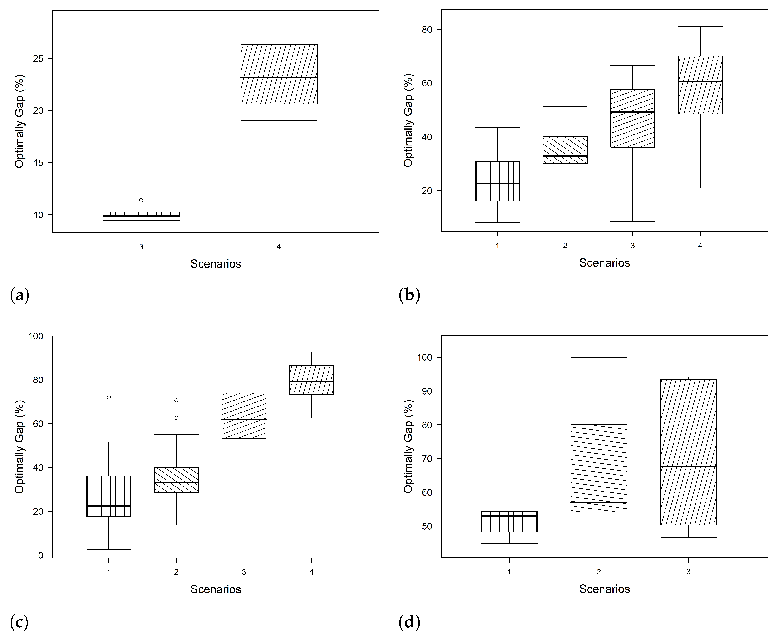
5.2. AMH Performance

The AMH was tested with all the instances studied in the literature, and it was able to find feasible solutions for all of them. However, when using the optimization models, there are some instances for which the solver did not report a feasible solution. Therefore, to gain insight into the quality of the AMH solutions, we analyzed only the instances for which there is a best-known solution. The best-known is the best solution reported by CPLEX in the SLAUPR, SLAUPR_V2, or SLAUPR_V3 models.
Table 5 shows the proposed AMH performance. Column Best-known F/O describes the number of instances with the best-known feasible solutions and the number of optimal ones found. Column AMH F/O describes the number of instances with a feasible solution and the number of instances solved optimally by our AMH. Column Average time (s) represents the average execution time to find the best-known solution and to report feasible solutions to the proposed AMH, respectively. Column Average Gap E , A (%) is the average gap between the best-known feasible solutions and the best-found solution generated by AMH. The Gap E , A (%) is calculated as follows:
Gap E , A ( % ) = 100 × Z E Z A Z E ,
where Z E and Z A represent the value of the best-known solution when solving the mathematical models with CPLEX and the AMH, respectively. A negative Gap E , A indicates that the results by the models are better. Otherwise, the AMH reports better results.
Table 5 shows that the solutions found by the proposed algorithm are competitive compared to the results with the best-known solutions. Note that the best performance of the AMH was in the set of small and medium type_1 instances since 100% (72/72) and 86.9% (53/61) of the known optimal solutions were obtained, respectively. For the medium instances type_2, although the AMH did not find any optimal solution, it improved more than 27% and 59% of the best-known feasible solutions in scenario_2 and scenario_4, respectively. For large instances, the AMH enhances approximately 78% and 67% solutions in scenario_2 and scenario_3, respectively.
One of the main advantages of the proposed AMH is that, for the first time, we could find a feasible solution for the most complex instances reported in the literature. Although the AMH did not find all the optimal solutions, this algorithm considerably improves more than 29% of the best-known feasible solutions, besides finding the same solution in 40% of the cases. For all the tested instances, the average general execution time to report feasible solutions is 117 s.

5.3. MIPStart Analysis

To accelerate the solver convergence and increase the number of instances with optimal solutions, we used the solution reported by our AMH as an initial solution to feed the solver when solving the problem with the different models we have. This process is referred to as MIPStart. Note that we used the same instance set as in the previous section.
The results of the MIPStart process are shown in Table 6. The column Average improvement Δ Gap E , M (%) refers to the average solution improvement between the original model and the one MIPStart. Δ Gap E , M (%) is computed as follows:
Δ Gap E , M ( % ) = 100 × Z E Z M Z E ,
where Z E and Z M represent the value of the solution when solving the mathematical models without an initial solution and with an initial solution, respectively.
Figure 2 shows the relative gap reported by CPLEX of the best-found feasible solution (without including optimal ones) when solving the SLAUPR_V2 or the SLAUPR_V3 with MIPStart.
It can be observed, for small instances, that scenario_1 and scenario_2 are the least complex, and the initial solution matches the optimal solution. Therefore, there are no improvements due to the MIPStart. Although this size presents a low complexity, the scenarios that show greater complexity are 3 and 4. Based on Figure 2a, the optimality gap remains below 30% in most instances, with maximums of 11% and 27% for scenario_3 and scenario_4, respectively.
MIPStart significantly improved the solution found for the medium type_1, medium type_2, and large instances compared to the models without initial conditions. MIPStart of the SLAUPR model presents a greater impact on the convergence of the optimizer for the medium type_1 and medium type_2 size instances. In contrast, for the large instances, the highest percentage of the average improvement of the solution is reached by MIPStart of the SLAUPR_V2 model (82.29%) in scenario_2 and the SLAUPR_V3 model (73.69%) in scenario_3.
Based on the best-found MIPStart solution, Figure 2b shows that for the most complex scenarios, in this case, scenario_3 and scenario_4 of medium type_1, instances are left with maximum optimality gaps of 66% and 81% and with minimums of 9% and 19%, respectively. Although for the medium type_2 and large instances, all four scenarios are still very complex, Figure 2c shows that for scenario_1, a minimum gap is reported by CPLEX of 3%, and for 50% of the tested instances it oscillates from 18% to 35%, and for scenario_2, from 30% to 40%. For scenario_3, around 25% of the instances present an optimality gap from 65% to 75%. For scenario_4, the minimum gap is 60%. Although it continues without solving optimality in some large instances, as seen in Figure 2, a minimum optimality gap of 45% and maximums greater than 50% are reported.

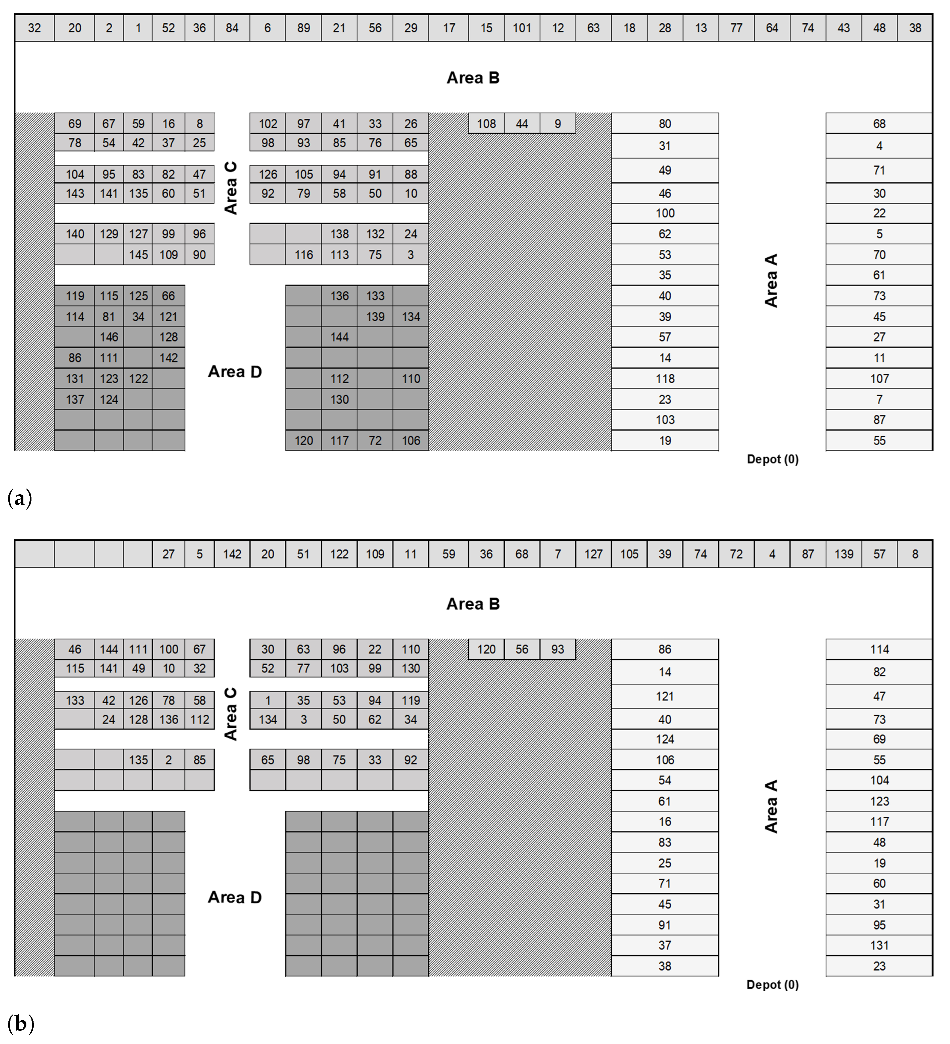
5.4. Comparison of the Real Situation and AMH Solution

To determine the improvements provided by our AMH, we analyze one large instance (based on real data). In Figure 3, we present a comparison of storage location and travel times based on the current location of the company and the allocation obtained by our AMH.
Figure 3a shows that with the allocation of the company, there is a dispersion of the products in the warehouse. In contrast, the allocation obtained by our AMH presents a group of the most compact products (see Figure 3b). Therefore, the shortest travel time is achieved by our proposed algorithm since the relocation of all the analyzed products simultaneously considers the assignment of the best candidate product through the evaluation function described in the expression (23) and the choice of the nearest adjacent location.
The total travel time on the route is reduced by more than 40%, which means this activity can be carried out faster without affecting the final product (customer order). Similarly, the pickers will not have to choose alternate routes and will not incur extra costs to fulfill orders.
The results of this study highlight the importance of integrating storage location and picker-routing decisions, the same as the work of [11,27]. While previous works have typically addressed these problems separately, assuming that storage location decisions are long term and resistant to change, practical considerations in certain industries and businesses may require more dynamic approaches. Factors such as seasonality and product life cycles can influence product demand and require periodic reviews of storage location decisions. Although concerns about relocation costs are an argument to avoid periodic reassignments of products to storage locations, our experimental findings demonstrate the benefits of adjusting storage and routing decisions to minimize travel time in the order-picking process. Therefore, decision makers must acknowledge and consider the interdependence between the two problems, which may seem intuitive but warrants careful attention.

6. Conclusions

We studied the storage location and the picker-routing problems, recently introduced in the literature as SLAUPR. We proposed and tested two different formulations for SLAUPR: SLAUPR_V2 adds some valid inequalities, and SLAUPR_V3 considers single commodity flow constraints for sub-tour elimination. Additionally, we proposed one adaptive multi-start heuristics (AMH) to improve the case study results reported in the literature.
The results show the excellent performance of our models and algorithm. With the reformulations, we achieved 62 new feasible and 51 optimal ones for the existing instances in the literature, which were obtained mainly from the SLAUPR_V3 model, which indicates the good efficiency of the sub-tour elimination constraints based on flow versus MTZ constraints for these types of problems. On the other hand, AMH can generate feasible solutions for all the instances studied in the literature and improves (more than 29%) the best-known solutions. Moreover, the proposed AMH requires an average general execution time of 117 s to report feasible solutions. Consequently, we analyzed a MIPStart procedure, in which we feed the CPLEX solver with the solution reported by AMH to accelerate the convergence of CPLEX and to be able to compute the optimality gap of solutions.
Finally, comparing the allocated products that the company has with those obtained by the proposed heuristic, an improvement (more than 40%) in the picking times helps tactical decision making by providing the correct location of the products in the warehouse. The proposed AMH is an excellent alternative for any company interested in solving the storage location assignment and the picker-routing problem in consideration of the weight of the products.
It is important to point out that decision makers need to analyze the trade-off between optimal and approximated solutions to speed up their practical implementation since finding an optimal solution may be impractical due to the complexity of the problem.
Future work could focus on the study of an extension of the problem by integrating batching decisions and considering stochastic demands or inventory replenishment under supply uncertainty.

Author Contributions

Editing and writing, J.B.-Z., M.A.S.-A. and J.A.S.-M.; methodology, J.B.-Z., M.A.S.-A. and J.A.S.-M., experimentation, J.B.-Z.; formal analysis, J.B.-Z., M.A.S.-A. and J.A.S.-M.; supervision, M.A.S.-A. and J.A.S.-M. All authors have read and agreed to the published version of the manuscript.

Funding

This research was funded by UANL, PAICYT grants CE1819-21 and 547-IT-2022.

Data Availability Statement

The authors can provide the data used in this study upon request.

Acknowledgments

The first author sincerely thanks CONAHCYT (National Council of Humanities, Science, and Technology from Mexico) and FIME-UANL for granted scholarship.

Conflicts of Interest

The authors declare no conflict of interest.

References

  1. Bartholdi, J.; Hankman, S. Warehouse and Distribution Science Release 0.96. 2014. Available online: https://www.warehouse-science.com/book/index.html (accessed on 2 November 2021).
  2. Davarzani, H.; Norrman, A. Toward a relevant agenda for warehousing research: Literature review and practitioners’ input. Logist. Res. 2015, 8, 1. [Google Scholar] [CrossRef] [Green Version]
  3. Henn, S.; Schmid, V. Metaheuristics for order batching and sequencing in manual order picking systems. Comput. Ind. Eng. 2013, 66, 338–351. [Google Scholar] [CrossRef]
  4. Casella, G.; Volpi, A.; Montanari, R.; Tebaldi, L.; Bottani, E. Trends in order picking: A 2007–2022 review of the literature. Prod. Manuf. Res. 2023, 11, 2191115. [Google Scholar] [CrossRef]
  5. Daniels, R.L.; Rummel, J.L.; Schantz, R. A model for warehouse order picking. Eur. J. Oper. Res. 1998, 105, 1–17. [Google Scholar] [CrossRef]
  6. Petersen, C. The impact of routing and storage policies on warehouse efficiency. Int. J. Oper. Prod. Manag. 1999, 19, 1053–1064. [Google Scholar] [CrossRef]
  7. Kordos, M.; Boryczko, J.; Blachnik, M.; Golak, S. Optimization of Warehouse Operations with Genetic Algorithms. Appl. Sci. 2020, 10, 4817. [Google Scholar] [CrossRef]
  8. Venkata, R.M.; Gajendra, K.A. Class-based storage-location assignment to minimise pick travel distance. Int. J. Logist. Res. Appl. 2008, 11, 247–265. [Google Scholar] [CrossRef]
  9. van Gils, T.; Ramaekers, K.; Caris, A.; de Koster, R.B.M. Designing efficient order picking systems by combining planning problems: State-of-the-art classification and review. Eur. J. Oper. Res. 2018, 267, 1–15. [Google Scholar] [CrossRef] [Green Version]
  10. Van Gils, T.; Ramaekers, K.; Braekers, K.; Depaire, B.; Caris, A. Increasing order picking efficiency by integrating storage, batching, zone picking, and routing policy decisions. Int. J. Prod. Econ. 2018, 197, 243–261. [Google Scholar] [CrossRef]
  11. Silva, A.; Coelho, L.C.; Darvish, M.; Renaud, R. Integrating storage location and order picking problems in warehouse planning. Transp. Res. Part E Logist. Transp. Rev. 2020, 140, 102003. [Google Scholar] [CrossRef]
  12. Salhi, S.; Nagy, G. Consistency and robustness in location-routing. In Studies in Locational Analysis; University of Kentucky: Lexington, KY, USA, 1999; pp. 3–19. [Google Scholar]
  13. Winkelhaus, S.; Grosse, E.H.; Morana, S. Towards a conceptualisation of Order Picking 4.0. Comput. Ind. Eng. 2021, 159, 107511. [Google Scholar] [CrossRef]
  14. Dekker, R.; de Koster, R.B.M.; Roodbergen, K.J.; Van, K.H. Improving Order Picking Response Time at Ankor’s Warehouse. Interfaces 2004, 34, 303–313. [Google Scholar] [CrossRef] [Green Version]
  15. Žulj, I.; Glock, C.H.; Grosse, E.H.; Schneider, M. Picker routing and storage-assignment strategies for precedence-constrained order picking. Comput. Ind. Eng. 2018, 123, 338–347. [Google Scholar] [CrossRef]
  16. Chabot, T.; Lahyani, R.; Coelho, L.C.; Renaud, J. Order picking problems under weight, fragility and category constraints. Int. J. Prod. Res. 2017, 55, 6361–6379. [Google Scholar] [CrossRef]
  17. Zunic, E.; Besirevic, A.; Skrobo, R.; Hasic, H.; Hodzic, K.; Djedovic, A. Design of optimization system for warehouse order picking in real environment. In Proceedings of the 2017 XXVI International Conference on Information, Communication and Automation Technologies (ICAT), Sarajevo, Bosnia and Herzegovina, 26–28 October 2017; IEEE: Toulouse, France, 2017; pp. 1–6. [Google Scholar] [CrossRef]
  18. Bolaños-Zuñiga, J.; Saucedo-Martínez, J.A.; Salais-Fierro, T.E.; Marmolejo-Saucedo, J.A. Optimization of the storage location assignment and the picker-routing problem by using mathematical programming. Appl. Sci. 2020, 10, 534. [Google Scholar] [CrossRef] [Green Version]
  19. Gavish, B.; Graves, S. The Traveling Salesman Problem and Related Problems; Working Paper GR-078-78; Massachusetts Institute of Technology, Operations Research Center: Cambridge, MA, USA, 1978. [Google Scholar]
  20. Caron, F.; Marchet, G.; Perego, A. Routing policies and COI-based storage policies in picker-to-part systems. Int. J. Prod. Res. 1998, 36, 713–732. [Google Scholar] [CrossRef]
  21. Dijkstra, A.S.; Roodbergen, K.J. Exact route-length formulas and a storage location assignment heuristic for picker-to-parts warehouses. Transp. Res. Part Logist. Transp. Rev. 2017, 102, 38–59. [Google Scholar] [CrossRef]
  22. Çelk, M.; Süral, H. Order picking under random and turnover-based storage policies in fishbone aisle warehouses. IIE Trans. 2014, 46, 283–300. [Google Scholar] [CrossRef]
  23. Wan, Y.; Liu, Y. Integrating Optimized Fishbone Warehouse Layout, Storage Location Assignment and Picker Routing. IAENG Int. J. Comput. Sci. 2022, 49, 957–974. [Google Scholar]
  24. Zhou, L.; Zhao, J.; Liu, H.; Wang, F.; Jianglong, Y.; Wang, S. Stochastic models of routing strategies under the class-based storage policy in fishbone layout warehouses. Sci. Rep. 2022, 12, 17. [Google Scholar] [CrossRef]
  25. Glock, C.H.; Grosse, E.H.; Abedinnia, H.; Emde, S. An integrated model to improve ergonomic and economic performance in order picking by rotating pallets. Eur. J. Oper. Res. 2019, 273, 516–534. [Google Scholar] [CrossRef]
  26. Castier, M.; Martínez-Toro, E. Planning and picking in small warehouses under industry-relevant constraints. Prod. Eng. 2023, 17, 575–590. [Google Scholar] [CrossRef]
  27. Cai, J.; Xiaokang, L.; Yue, L.; Ouyang, S. Collaborative Optimization of Storage Location Assignment and Path Planning in Robotic Mobile Fulfillment Systems. Sustainability 2021, 13, 5644. [Google Scholar] [CrossRef]
  28. Keung, K.; Lee, C.; Ji, P. Industrial internet of things-driven storage location assignment and order picking in a resource synchronization and sharing-based robotic mobile fulfillment system. Adv. Eng. Informatics 2022, 52, 101540. [Google Scholar] [CrossRef]
  29. Sarkar, B.; Takeyeva, D.; Guchhait, R.; Sarkar, M. Optimized radio-frequency identification system for different warehouse shapes. Knowl.-Based Syst. 2022, 258, 109811. [Google Scholar] [CrossRef]
  30. Scholz, A.; Henn, S.; Stuhlmann, M.; Wäscher, G. A new mathematical programming formulation for the Single-Picker Routing Problem. Eur. J. Oper. Res. 2016, 253, 68–84. [Google Scholar] [CrossRef]
  31. Theys, C.; Bráysy, O.; Dullaert, W.; Raa, B. Using a TSP heuristic for routing order pickers in warehouses. Eur. J. Oper. Res. 2010, 200, 755–763. [Google Scholar] [CrossRef]
  32. Lin, C.C.; Kang, J.R.; Hou, C.C.; Cheng, C.Y. Joint order batching and picker Manhattan routing problem. Comput. Ind. Eng. 2016, 95, 164–174. [Google Scholar] [CrossRef]
  33. Ratliff, H.D.; Rosenthal, A.S. Order-Picking in a Rectangular Warehouse: A Solvable Case of the Traveling Salesman Problem. Oper. Res. 1983, 31, 507–521. [Google Scholar] [CrossRef]
  34. Scholz, A.; Wäscher, G. Order Batching and Picker Routing in manual order picking systems: The benefits of integrated routing. Cent. Eur. J. Oper. Res. 2017, 25, 491–520. [Google Scholar] [CrossRef]
  35. Xu, X.; Ren, C. A novel storage location assignment in multi-pickers picker-to-parts systems integrating scattered storage, demand correlation, and routing adjustment. Comput. Ind. Eng. 2022, 172, 108618. [Google Scholar] [CrossRef]
  36. Bottani, E.; Cecconi, M.; Vignali, G.; Montanari, R. Optimisation of storage allocation in order picking operations through a genetic algorithm. Int. J. Logist. Res. Appl. 2012, 15, 127–146. [Google Scholar] [CrossRef]
  37. Sarkar, A.; Guchhait, R.; Sarkar, B. Application of the Artificial Neural Network with Multithreading Within an Inventory Model Under Uncertainty and Inflation. Int. J. Fuzzy Syst. 2022, 24, 2318–2332. [Google Scholar] [CrossRef]
  38. Singh-Padiyar, S.V.; Vandana, V.; Bhagat, N.; Singh, S.R.; Sarkar, B. Joint replenishment strategy for deteriorating multi-item through multi-echelon supply chain model with imperfect production under imprecise and inflationary environment. RAIRO-Oper. Res. 2022, 56, 3071–3096. [Google Scholar] [CrossRef]
  39. Lee, H.T. Travel distance estimation of relation-based storage assignment policies in picker-to-part warehouses. J. Bus. Adm. 2022, 47, 17. [Google Scholar] [CrossRef]
  40. Alqahtani, A. Improving order-picking response time at retail warehouse: A case of sugar company. SN Appl. Sci. 2023, 5, 8. [Google Scholar] [CrossRef]
  41. Cortés, P.; Gómez-Montoya, R.A.; Muñuzuri, J.; Correa-Espinal, A. A tabu search approach to solving the picking routing problem for large- and medium-size distribution centres considering the availability of inventory and K heterogeneous material handling equipment. Appl. Soft Comput. 2017, 53, 61–73. [Google Scholar] [CrossRef]
  42. Wang, W.; Gao, J.; Gao, T.; Zhao, H. Optimization of Automated Warehouse Location Based on Genetic Algorithm. In Proceedings of the 2017 2nd International Conference on Control, Automation and Artificial Intelligence (CAAI 2017), Sanya, China, 25–26 June 2017; Atlantis Press: Paris, France, 2017. [Google Scholar] [CrossRef]
  43. Eydi, A.; Mohagheghi, H.; Ghaseminezhad, S. Routing order pickers in warehouses considering congestion and aisle width. Sci. Iran. 2020, 29, 3455–3469. [Google Scholar] [CrossRef]
  44. Boudia, M.; Louly, M.; Prins, C. A reactive GRASP and path relinking for a combined production–distribution problem. Comput. Oper. Res. 2007, 34, 3402–3419. [Google Scholar] [CrossRef]
  45. Cantu-Funes, R.; Salazar-Aguilar, M.A.; Boyer, V. Multi-depot periodic vehicle routing problem with due dates and time windows. J. Oper. Res. Soc. 2018, 69, 296–306. [Google Scholar] [CrossRef]
  46. Edis, E.; Uzun Araz, O.; Eski, O.; Edis, R. Storage location assignment of steel coils in a manufacturing company: An integer linear programming model and a greedy randomized adaptive search procedure. TOP 2023, 31, 67–109. [Google Scholar] [CrossRef]
  47. Feo, T.A.; Resende, M.G.C. Greedy randomized adaptive search procedures. J. Glob. Optim. 1995, 6, 109–133. [Google Scholar] [CrossRef] [Green Version]
  48. Prais, M.; Ribeiro, C.C. Reactive grasp: An application to a matrix decomposition problem in TDMA traffic assignment. INFORMS J. Comput. 2000, 12, 164–176. [Google Scholar] [CrossRef] [Green Version]
  49. Hota, S.K.; Ghosh, S.K.; Sarkar, B. A solution to the transportation hazard problem in a supply chain with an unreliable manufacturer. AIMS Environ. Sci. 2022, 9, 354–380. [Google Scholar] [CrossRef]
  50. Azadnia, A.H.; Taheri, S.; Ghadimi, P.; Mat, S.; Muhamad, Z.; Wong, K.Y. Order batching in warehouses by minimizing total tardiness: A hybrid approach of weighted association rule mining and genetic algorithms. Sci. World J. 2013, 2013, 246578. [Google Scholar] [CrossRef]
  51. Miller, C.E.; Tucker, A.; Zemlin, R. Integer Programming Formulation of Traveling Salesman Problems. J. Assoc. Comput. Mach. 1960, 7, 326–329. [Google Scholar] [CrossRef]
  52. Palomo-Martínez, P.; Salazar-Aguilar, M.; Albornoz, V. Formulations for the orienteering problem with additional constraints. Ann. Oper. Res. 2017, 258, 503–545. [Google Scholar] [CrossRef]
  53. Chaovalitwongse, W.; Kim, D.; Pardalos, P.M. Grasp with a new local search scheme for vehicle routing problems with time window. J. Comb. Optim. 2003, 7, 179–207. [Google Scholar] [CrossRef]
  54. Villegas, J.G.; Prins, C.; Prodhon, C.; Medaglia, A.; Velasco, N. A GRASP with evolutionary path relinking for the truck and trailer routing problem. Comput. Oper. Res. 2011, 38, 1319–1334. [Google Scholar] [CrossRef]
  55. Haddadene, S.R.A.; Labadie, N.; Prodhon, C. A GRASP × ILS for the vehicle routing problem with time windows, synchronization and precedence constraints. Expert Syst. Appl. 2016, 66, 274–294. [Google Scholar] [CrossRef]
  56. Festa, P.; Resende, M.G.C. GRASP: Basic components and enhancements. Telecommun. Syst. 2010, 46, 253–271. [Google Scholar] [CrossRef] [Green Version]
Figure 1. Warehouse layout of the case study from the literature [18].
Axioms 12 00711 g001
Figure 2. Optimality gap reported by CPLEX of the best-found solution MIPStart. (a) Small size instances. (b) Medium type_1 size instances. (c) Medium type_2 size instances. (d) Large size instances.
Axioms 12 00711 g002
Figure 3. Location of products in the warehouse. (a) Current assignment of the company—Travel time: 4.274 s. (b) Assignment proposed by AMH—Travel time: 2.446 s.
Axioms 12 00711 g003
Table 2. Notation used in mathematical models and the heuristic approach.
Index Sets
IStore locations including the depot
KAvailable products in the warehouse
PRequested orders
X K Products to assign
Parameters
d k p Demand of product k K in order p P
Q j k Physical capacity of location j I to store product k K
t i j Time matrix between locations ( i , j I )
w k Weight of product k K
M p j k min { d k p , Q j k }
M max k K { w k }
Decision variables
u p i j = 1 , if a picker visits location j after location i ( i , j I ) while picking order p P 0 , otherwise
e j k = 1 , if location j I stores product k K 0 , otherwise
v p j k Number of boxes of product k K for picking in order p P at location j I .
s j p Auxiliary variable for subtour elimination constraints, it keeps the position in which                       
location j I is visited while picking order p P
Table 3. Instance description from [18].
Instance SizeStorage Location | I | Requested ProductsProducts to Assign | X | Orders to Pick | P | Number of Instances
Small10–1641–162–490
Medium type_1328–165–321–5144
Medium type_26115–3012–611–575
Large121–1853025–1041–625
Table 4. Summary solutions reported by [18] against the ones obtained by the proposed mathematical reformulations.
Size
Instance
ScenariosSLAUPRSLAUPR_V2SLAUPR_V3
F/OAverage
Optimality Gap (%)
F/OAverage
Optimality Gap (%)
F/OAverage
Optimality Gap (%)
Small124/240.0024/240.0024/240.00
224/240.0024/240.0024/240.00
318/633.4718/1219.2418/123.83
424/635.9224/1223.2724/128.48
Totals90/60 90/72 90/72
Medium
type_1
130/332.1131/237.6834/256.15
230/1622.6233/2413.1336/2415.63
317/1214.2117/1215.2027/1223.54
46/063.4914/074.4319/054.98
Totals83/32 95/59 116/61
Medium
type_2
118/081.8117/057.1525/034.94
224/088.5126/073.1725/057.53
37/153.417/422.448/337.78
40/0-0/0 1/081.04
Totals49/1 50/4 59/3
Large10/0-0/0-0/0-
23/094.686/099.290/0-
32/083.161/098.234/087.55
Totals5/0 7/0 4/0
Totals227/87 242/135 269/136
Table 5. Gap between the best-known feasible solutions and the proposed AMH.
Size
Instance
ScenariosBest-KnownAMHAverage   Gap E , A (%)
F/OAverage
Time (s)
F/OAverage
Time (s)
Small124/24024/2480
224/24024/2440
318/12120918/1212−2.46
424/12183324/12160.16
Totals90/7273190/7210
Medium
type_1
136/25114536/2419−3.12
236/24121136/23133.15
327/12204736/653−5.57
425/0360036/07827.42
Totals124/611855144/5341
Medium
type_2
126/0720028/0475.47
228/0705428/03727.89
39/5588211/0202−7.91
41/072008/049659.87
Totals64/5695175/0114
Large10/0 4/0107
26/011,04015/012178.72
35/010,8006/011466.92
Totals11/010,80025/0117
Totals289/138 334/125
Table 6. Summary results of MIPStart models.
Size
Instance
ScenariosAverage Improvement
Δ Gap E , M (%)
SLAUPRSLAUPR_V2SLAUPR_V3
Small1000
2000
35.840.500.28
42.721.670.80
Medium
type_1
18.80.411.98
212.523.678.12
31.422.8310.75
430.1135.0326.08
Medium
type_2
159.0116.0315.9
274.135.8735.95
347.5215.4131.46
4--59.87
Large275.9782.29-
360.1372.0173.69
Disclaimer/Publisher’s Note: The statements, opinions and data contained in all publications are solely those of the individual author(s) and contributor(s) and not of MDPI and/or the editor(s). MDPI and/or the editor(s) disclaim responsibility for any injury to people or property resulting from any ideas, methods, instructions or products referred to in the content.

