Article

Constant-Stress Modeling of Log-Normal Data under Progressive Type-I Interval Censoring: Maximum Likelihood and Bayesian Estimation Approaches

1
State Key Laboratory of Mechanics and Control of Mechanical Structures, Institute of Nano Science and Department of Mathematics, Nanjing University of Aeronautics and Astronautics, Nanjing 210016, China
2
Department of Mathematics, Faculty of Science, Fayoum University, Fayoum 63514, Egypt
3
Department of Mathematics, Faculty of Science for Girls, King Khalid University, Abha 61413, Saudi Arabia
4
Department of Mathematics, Faculty of Education, Ain Shams University, Cairo 11566, Egypt
*
Author to whom correspondence should be addressed.
Axioms 2023, 12(7), 710; https://doi.org/10.3390/axioms12070710
Submission received: 22 June 2023 / Revised: 15 July 2023 / Accepted: 17 July 2023 / Published: 21 July 2023

Abstract

:
This paper discusses inferential approaches for the problem of constant-stress accelerated life testing when the failure data are progressive type-I interval censored. Both frequentist and Bayesian estimations are carried out under the assumption that the log-normal location parameter is nonconstant and follows a log-linear life-stress model. The confidence intervals of unknown parameters are also constructed based on asymptotic theory and Bayesian techniques. An analysis of a real data set is combined with a Monte Carlo simulation to provide a thorough assessment of the proposed methods.

1. Introduction

Accelerated life testing (ALT) is a valuable technique used in manufacturing design to test the reliability and longevity of products in a cost-effective and efficient manner. ALTs involve subjecting the units to higher-than-use stress conditions, thereby accelerating the aging and failure processes, and then estimating the lifetime distribution features at the use condition through a statistically appropriate model. The constant-stress ALT (CS-ALT) model is one of the two main methods used in ALTs. In this method, the units are subjected to a constant stress level throughout the test cycle. The second method is the step-stress model, which involves subjecting the units to a series of increasing stress levels in a stepwise manner. For an extensive coverage of various aspects of the ALT models, including test designs, data analysis methods, and reliability estimation, one can consult the monographs written by Nelson [1], Meeker and Escobar [2], Bagdonavicius and Nikulin [3], and Limon et al. [4].
Most test plans that are published use the concepts of type-I or type-II censoring for testing items under design stress in an accelerated setting. Type-I censoring involves stopping testing after a fixed duration, which provides the advantage of a precise experiment duration but leads to uncertainty about the number of failures observed. On the other hand, type-II censoring involves stopping testing after a predetermined number of failures, which provides certainty about the number of failures but leads to uncertainty about the experiment’s duration. In reliability testing, type-II censoring schemes are often employed when conducting experiments to determine the reliability or failure rate of a product or system. Type-II censoring occurs when the experiment is terminated after a predetermined number of failures, and the remaining items are considered censored observations. In this context, Zheng [5] expressed the asymptotic Fisher information for type-II censored data, relating it to the hazard function. Additionally, they demonstrated that the factorization of the hazard function can be characterized by the linear property of the Fisher information in the context of type-II censoring. Moreover, Xu and Fei [6] explored theories related to the approximate optimal design for a simplified step-stress ALT method under type-II censoring. The researchers develop statistically approximated optimal ALT plans with the objective of minimizing the asymptotic variance of the maximum likelihood estimators for the p-th percentile of lifetime at the design stress level. Utilizing data from CS-ALT experiments with type-II censoring, Wenhui et al. [7] studied the interval estimate of the two-parameter exponential distribution. Furthermore, they derived generalized confidence intervals for the parameters in the life-stress model, including the location parameter, as well as the mean and reliability function at the designed stress level.
These two types of censoring are more distinct with smaller sample sizes, but their differences become less noticeable as the sample size increases. In this regard, several studies that are relevant to this issue at hand are present in Nelson and Kielpinski [8], Bai et al. [9], and Tang et al. [10], while the two types of censoring both have benefits, they share a significant disadvantage in that they permit the elimination of units solely after the conclusion of an experiment. In contrast, “progressive censoring”, which is a more comprehensive censoring approach, permits units to be removed during a test before its completion. For a more in-depth examination of progressive censoring, Balakrishnan and Aggarwala’s research [11] can be referenced. In certain situations, continuous monitoring of experiments to observe failure times is necessary. However, this may not always be feasible due to time and cost constraints. In such cases, the number of failures is recorded at predetermined time intervals, which is known as interval censoring. Aggarwala [12] developed a more generalized interval censoring scheme called progressive type-I interval censoring by combining interval censoring and progressive type-I censoring. In this scheme, the experimental units are observed at predetermined intervals, and only those units that have not failed up to a certain point are subjected to more frequent monitoring. This approach allows for more efficient use of resources and provides more precise estimates of failure times. Progressive type-I interval censoring has been the focus of significant attention by many authors in recent years. For instance, Chandrakant and Tripathi [13], Singh and Tripathi [14], Chen et al. [15], and Arabi Belaghi et al. [16] have conducted research and developed various methods for estimating the unknown parameters of different lifetime models under progressive type-I interval censoring scheme.
Several studies have been conducted on statistical inference for ALT models under different types of censoring schemes, such as type-I, type-II, and hybrid censoring (see, Abd El-Raheem [17,18,19], Sief et al. [20], Feng et al. [21], Balakrishnan et al. [22], and Nassar et al. [23]). However, the study of ALT models under a progressive type-I interval censoring scheme is still lacking in the literature, and as such, we aim to address this gap by exploring inferential approaches for CS-ALT models when the failure data are progressive type-I interval censored and are log-normally distributed.
The log-normal distribution is indeed widely used in failure time analysis and has proven to be a flexible and effective model for analyzing various physical phenomena. One notable characteristic of the log-normal distribution is that its hazard rate starts at zero, indicating a low failure rate at the beginning, then gradually increases to its maximum value, and eventually approaches zero as the variable x approaches infinity. This behavior makes the log-normal distribution suitable for modeling phenomena that exhibit initial low failure rates, followed by an increasing failure rate, and then a declining failure rate as time progresses. The applications of the log-normal distribution extend to various fields of study, including actuarial science, business, economics, and lifetime analysis of electronic components. Moreover, the log-normal distribution is valuable for analyzing both homogeneous and heterogeneous data. It can handle skewed data that may deviate from a normal distribution, making it suitable for modeling real-world datasets that exhibit asymmetry. This versatility has led to its application in a wide range of practical studies. One can refer to [24,25,26] for further insights into the applications of the log-normal distribution in various fields and to demonstrate its usefulness in analyzing different types of data.
Assuming that the lifetime of the test units represented by a random variable T follows a log-normal distribution with a nonconstant location parameter < μ < is affected by stress and a scale parameter σ > 0 , then probability density function (PDF) and the cumulative distribution function (CDF) of the log-normal distribution can be expressed as follows:
f ( t ) = 1 2 π σ t exp ( ln ( t ) μ ) 2 2 σ 2 , t > 0 ,
F ( t ) = Φ ln ( t ) μ 2 σ .
where Φ ( · ) is the standard normal CDF.
The article is structured into several sections, which are summarized as follows: Section 2 provides a description of the test process and the assumptions that underlie it. In Section 3, the maximum likelihood estimates along with their associated asymptotic standard error are discussed. Section 4 focuses on the discussion of Bayesian estimation techniques. The proposed methods in Section 3 and Section 4 are then evaluated in Section 5 using simulation studies. Finally, Section 6 provides a summary of the findings as a conclusion.

2. Model and Underlying Assumptions

2.1. Model Description

In the CS-ALT method, the test units are divided into groups and each group is subjected to a higher stress level than the typical stress level. The stress levels are denoted as S 0 for the standard stress level and S 1 < S 2 < < S k for k different test stress levels. The data is collected using a progressive type-I interval censored sampling approach for each stress level S i , i = 1 , 2 , , k .
In this approach, a set of n i identical units is simultaneously tested at time t i 0 = 0 for each stress level S i . Inspections are performed at predetermined times t i 1 < t i 2 < < t i m i , with t i m i being the planned end time of the experiment. During each inspection, the number of failed units X i j within the interval ( t i ( j 1 ) , t i j ] is recorded. Additionally, at each inspection time t i j , a random selection process eliminates R i j surviving units from the test, where R i j should not exceed the number of remaining units Y i j . The value of R i j is determined as a specified percentage p i j of the remaining units at t i j , using the formula R i j = p i j × y i j , where j = 1 , 2 , , m i . The percentage values p i j are pre-specified, with p i m i = 1 , indicating that all remaining units are eliminated at the final inspection time.
In this scenario, a progressive type-I interval censored sample of size n i can be represented as:
D = X i j , R i j , t i j , i = 1 , 2 , , k , j = 1 , 2 , , m i .
Here, the total sample size n is given by the sum of the number of units in each stress level, which is defined as n = i = 1 k n i = i = 1 k j = 1 m i ( X i j + R i j ) .

2.2. Basic Assumptions

In the CS-ALT context, the following assumptions are considered:
  • The lifetime of test units follows a log-normal distribution at stress level S i , with PDF given by
    f i ( t ) = 1 2 π σ t exp ( ln ( t ) μ i ) 2 2 σ 2 .
  • For the log-normal location parameter μ i , the life-stress model is assumed to be log-linear, i.e., it is described as
    log ( μ i ) = a + b S i , i = 0 , 1 , , k .
Here, a and b (where b < 0 ) are unknown coefficients that dependent on the product’s nature and the test method used. Using this log-linear model, μ i can be further expressed as μ i = μ 0 e b ( S i S 0 ) = μ 0 θ h i , where μ 0 represents the location parameter of the log-normal distribution under the reference stress level S 0 . Additionally, θ = e b ( S k S 0 ) = μ k μ 0 < 1 , and h i = S i S 0 S k S 0 satisfies h k > h k 1 > > h 1 = 1 . These assumptions provide the basis for analyzing and modeling the lifetime behavior of test units under different stress levels in CS-ALT experiments. Further details can be found in Chapter 2 of Nelson’s book [1].

3. Maximum Likelihood Estimation

Based on the observed lifetime data D and the assumptions 1 and 2, the likelihood function for μ 0 , σ and θ is given by:
L ( μ 0 , σ , θ | D ) i = 1 k j = 1 m i F t i j ; μ 0 , σ , θ F t i ( j 1 ) ; μ 0 , σ , θ X i j 1 F t i j ; μ 0 , σ , θ R i j i = 1 k j = 1 m i Φ τ i j Φ τ i ( j 1 ) X i j 1 Φ τ i j R i j ,
where τ i j = ln ( t i j ) μ i σ .
The corresponding log-likelihood function denoted by L = ln L ( μ 0 , σ , θ | D ) . When the partial derivatives of L with respect to μ 0 , σ , and θ are set to zero, the maximum likelihood estimators (MLEs) of μ 0 , σ , and θ can then be obtained by simultaneously solving the following equations:
L μ 0 = 1 σ i = 1 k X i 1 θ h i ϕ τ i 1 Φ τ i 1 1 σ i = 1 k j = 2 m i X i j θ h i ψ i j ψ i ( j 1 ) + 1 σ i = 1 k j = 1 m i R i j θ h i φ i j = 0 , L θ = 1 σ θ i = 1 k X i 1 h i μ i ϕ τ i 1 Φ τ i 1 1 σ θ i = 1 k j = 2 m i X i j h i μ i ψ i j ψ i ( j 1 ) + 1 σ θ i = 1 k j = 1 m i R i j h i μ i φ i j = 0 , L σ = 1 σ i = 1 k X i 1 τ i 1 ϕ τ i 1 Φ τ i 1 1 σ i = 1 k j = 2 m i X i j τ i j ψ i j τ i ( j 1 ) ψ i ( j 1 ) + 1 σ i = 1 k j = 1 m i R i j τ i j φ i j = 0 .
To simplify the expressions, we used the notations ψ i j = ϕ τ i j Φ τ i j Φ τ i ( j 1 ) and φ i j = ϕ τ i j 1 Φ τ i j . Here, ϕ ( · ) represents the standard normal PDF. Since the solutions to the aforementioned equations cannot be found in a closed form, the Newton–Raphson method is frequently employed in these circumstances to obtain the desired MLEs.

3.1. EM Algorithm

The expectation–maximization (EM) algorithm is a widely used tool for handling missing or incomplete data situations. It is a powerful iterative algorithm that seeks to maximize the likelihood function by estimating the missing data and the model parameters in an iterative manner. The EM algorithm is particularly useful when dealing with large amounts of missing data. Compared to other optimization methods such as the Newton–Raphson method, the EM algorithm is generally slower but more reliable in such cases.
The EM algorithm was first introduced by Dempster et al. [27], and has since been widely used in many different fields. McLachlan and Krishnan [28] provide a comprehensive treatment of the EM algorithm, while Little and Rubin [29] have highlighted the advantages of the EM algorithm over other methods for handling missing data. Considering progressive type-I interval censoring, the complete sample W i under stress level S i can be expressed as W i = W i j , W i j * , where W i j = ( ω i j 1 , ω i j 2 , , ω i j X i j ) represent the lifetimes of the units within the jth interval ( t i ( j 1 ) , t i j ] and W i j * = ( ω i j 1 * , ω i j 2 * , , ω i j R i j * ) denote to the lifetimes for the units that were removed at time t i j , for j = 1 , 2 , , m i . As a result, we can express the log-likelihood function of the complete data set as
L C W ; μ 0 , σ , θ i = 1 k j = 1 m i x = 1 X i j ln f ( ω i j x ; μ 0 , σ , θ ) + r = 1 R i j ln f ( ω i j r * ; μ 0 , σ , θ ) = n ln ( σ ) μ 0 2 2 σ 2 i = 1 k n i θ 2 h i + μ 0 σ 0 2 i = 1 k j = 1 m i θ h i x = 1 X i j ln ω i j x + r = 1 R i j ln ω i j r * 1 2 σ 0 2 i = 1 k j = 1 m i x = 1 X i j ln 2 ω i j x + r = 1 R i j ln 2 ω i j r * i = 1 k j = 1 m i x = 1 X i j ln ω i j x + r = 1 R i j ln ω i j r * .
By taking partial derivatives of Equation (6) with respect to μ 0 , σ , and θ , we can obtain the associated log-likelihood equations as follows:
μ 0 i = 1 k n i θ 2 h i = i = 1 k j = 1 m i θ h i x = 1 X i j ln ω i j x + r = 1 R i j ln ω i j r * ,
μ 0 i = 1 k n i h i θ 2 h i = i = 1 k j = 1 m i h i θ h i x = 1 X i j ln ω i j x + r = 1 R i j ln ω i j r * ,
n σ 2 + μ 0 2 i = 1 k n i θ 2 h i = i = 1 k j = 1 m i x = 1 X i j ln 2 ω i j x + r = 1 R i j ln 2 ω i j r * .
In the EM algorithm, two main steps are involved: The expectation step (E-step) and the maximization step (M-step). In the E-step, the observed and censored observations are replaced by their respective expected values. This step helps in estimating the missing or censored data. The process of finding the expected values in the E-step of the EM algorithm in our case involves calculating the expectations of four quantities
E 1 i j μ 0 , σ , θ = E ln [ W i j ] | t i ( j 1 ) < W i j t i j ; μ 0 , σ , θ , E 2 i j μ 0 , σ , θ = E ln [ W i j * ] | W i j * > t i j ; μ 0 , σ , θ , E 3 i j μ 0 , σ , θ = E ln 2 [ W i j ] | t i ( j 1 ) < W i j t i j ; μ 0 , σ , θ , E 4 i j μ 0 , σ , θ = E ln 2 [ W i j * ] | W i j * > t i j ; μ 0 , σ , θ .
Since W i j and W i j * are independent (see Ng et al. [30]), the process can be simplified using the following lemma (see Ng and Wang [31]).
Lemma 1. 
Given t i j and t i ( j 1 ) for i = 1 , 2 , , k and j = 1 , 2 , , m i , the conditional distributions of W and W * can be expressed as follows:
f W i j ( w ) = f ( w ) F ( t i j ) F ( t i ( j 1 ) ) , t i ( j 1 ) < w t i j , f W i j * ( w * ) = f ( w * ) 1 F ( t i j ) , w * > t i j .
Proof. 
The conditional distribution of W i j : the probability of W falling within the interval ( t i ( j 1 ) , t i j ] is given by:
P t i ( j 1 ) < W t i j = F ( t i j ) F ( t i ( j 1 ) ) ,
where F ( · ) is CDF of W. To normalize the distribution within this interval, the PDF of W is divided by the probability of W falling within the interval:
f W i j ( w ) = f ( w ) F ( t i j ) F ( t i ( j 1 ) ) , t i ( j 1 ) < w t i j .
This expression represents the conditional distribution of W i j . Similarly, we can directly deduce the conditional distribution of W i j * using a similar approach.    □
Thus, based on this result, we can readily acquire the necessary expected values in the following formulas.
E 1 i j μ 0 , σ , θ = μ i + σ ψ i ( j 1 ) ψ i j ,
E 2 i j μ 0 , σ , θ = μ i + σ φ i j ,
E 3 i j μ 0 , σ , θ = μ i 2 + 2 μ i σ ψ i ( j 1 ) ψ i j + σ 2 τ i ( j 1 ) ψ i ( j 1 ) τ i j ψ i j + 1 ,
E 4 i j μ 0 , σ , θ , = μ i 2 + 2 μ i σ φ i j + σ 2 τ i j φ i j + 1 .
Subsequently, during the M-step, the goal is to maximize the results obtained from the E-step. Thus, if we denote the estimate of ( μ 0 , σ , θ ) at the o-th stage as ( μ 0 ( o ) , σ ( o ) , θ ( o ) ) , applying the M-step will lead to updated estimates at the ( o + 1 ) -th stage. The updated estimates μ 0 ( o + 1 ) , θ ( o + 1 ) can be derived as the solution of the following equations.
μ 0 ( o + 1 ) i = 1 k n i ( θ ( o + 1 ) ) 2 h i = i = 1 k j = 1 m i ( θ ( o + 1 ) ) h i P i j ( o ) , μ 0 ( o + 1 ) i = 1 k n i h i ( θ ( o + 1 ) ) 2 h i = i = 1 k j = 1 m i h i ( θ ( o + 1 ) ) h i P i j ( o ) ,
where P i j ( o ) = X i j E 1 i j μ 0 ( o ) , σ ( o ) , θ ( o ) + R i j E 2 i j μ 0 ( o ) , σ ( o ) , θ ( o ) . While the updated value σ ( o + 1 ) can be obtained as
σ ( o + 1 ) = 1 n i = 1 k j = 1 m i Q i j ( o ) ( μ 0 ( ι + 1 ) ) 2 i = 1 k n i ( θ ( ι + 1 ) ) 2 h i 1 2 ,
where Q i j ( o ) = X i j E 3 i j μ 0 ( o ) , σ ( o ) , θ ( o ) + R i j E 4 i j μ 0 ( o ) , σ ( o ) , θ ( o ) . The iterative process continues until the desired convergence is achieved, which is determined by checking if the absolute differences between the updated and the previous values of μ 0 , σ , and θ are all less than or equal to a predefined value threshold ϵ > 0 . In mathematical terms, the convergence criterion is given by | μ 0 ( o + 1 ) μ 0 ( o ) | + | σ ( o + 1 ) σ ( o ) | + | θ ( o + 1 ) θ ( o ) | ϵ .

3.2. Midpoint Approximation Method

In this context, we assume that X i j of failures within each subinterval ( t i ( j 1 ) , t i j ] occurred at the midpoint of the interval, denoted as ς i j = 1 2 t i j + t i ( j 1 ) . Additionally, there are censored items R i j withdrawn at the censoring time t i j . Hence, the likelihood function can be approximated as:
L * ( μ 0 , σ , θ | D ) i = 1 k j = 1 m i f ς i j ; μ 0 , σ , θ X i j 1 F t i j ; μ 0 , σ , θ R i j .
The associated log-likelihood function for ( μ 0 , σ , θ ) is denoted as L * = ln L * ( μ 0 , σ , θ | D ) . To find the midpoint (MP) estimators of μ 0 , σ , and θ , we set the partial derivatives of L * with respect to μ 0 , σ , and θ to zero.
L * μ 0 = 1 σ i = 1 k j = 1 m i θ h i X i j τ i j * + R i j φ i j = 0 ,
L * θ = 1 σ θ i = 1 k j = 1 m i h i μ i X i j τ i j * + R i j φ i j = 0 ,
L * σ = 1 σ i = 1 k j = 1 m i X i j ( τ i j * 2 1 ) + R i j τ i j φ i j = 0 ,
where τ i j * = ln ( ς i j ) μ i σ . By simultaneously solving Equations (15)–(17), we can obtain the MP estimators for the parameters μ 0 , σ , and θ .
The advantage of the MP likelihood equations over the original likelihood equations is that they are often less complex and may lead to simpler numerical optimization procedures. This can enhance computational efficiency and facilitate the implementation of the estimation process.

3.3. Asymptotic Standard Errors

According to the missing information principle of Louis [32], the observed Fisher information matrix can be obtained as
I D ( Θ ) = I W ( Θ ) I W | D ( Θ ) ,
where Θ = ( μ 0 , σ , θ ) , I D ( Θ ) , I W ( Θ ) , and I W | D ( Θ ) represent observed information, complete, and missing information matrices. The complete information matrix, I W ( Θ ) , for the data from a log-normal distribution is provided by
I W ( Θ ) = E 2 L c ( W ; Θ ) Θ 2 = 1 σ 2 i = 1 k n i θ h i 0 1 θ i = 1 k n i h i μ i θ h i 0 n 0 1 θ i = 1 k n i h i μ i θ h i 0 1 θ 2 i = 1 k n i h i 2 μ i 2
Moreover, the missing information matrix I W | D ( Θ ) can be expressed as
I W | D ( Θ ) i = 1 k j = 1 m i X i j I W | D i j ( Θ ) + i = 1 k j = 1 m i R i j I W * | D i j ( Θ ) .
Here, I W | D i j ( Θ ) represents the information matrix for a single observation, conditioned on the event where t i ( j 1 ) < W t i j . Additionally, I W * | D i j ( Θ ) denotes the information matrix for a single observation that is censored at the failure time, t i j , conditioned on the event where W > t i j . The elements of both matrices can be obtained easily by utilizing Lemma 1 in the following manner:
I W | D i j ( Θ ) = E 2 log ( f W ( w ; Θ ) ) Θ 2 = p 11 p 12 p 13 p 21 p 22 p 23 p 31 p 32 p 33
where
p 11 = θ 2 h i σ 2 1 + τ i ( j 1 ) ψ i ( j 1 ) τ i j ψ i j ψ i ( j 1 ) ψ i j 2 , p 12 = θ h i σ 2 ψ i ( j 1 ) ψ i j + τ i ( j 1 ) 2 ψ i ( j 1 ) τ i j 2 ψ i j ψ i ( j 1 ) ψ i j τ i ( j 1 ) ψ i ( j 1 ) τ i j ψ i j , p 13 = h i μ i θ h i σ 2 θ 1 + τ i ( j 1 ) ψ i ( j 1 ) τ i j ψ i j ψ i ( j 1 ) ψ i j 2 , p 22 = 1 σ 2 2 + τ i ( j 1 ) ψ i ( j 1 ) τ i j ψ i j + τ i ( j 1 ) 3 ψ i ( j 1 ) τ i j 3 ψ i j ψ i ( j 1 ) ψ i j 2 , p 23 = h i μ i σ 2 θ ψ i ( j 1 ) ψ i j + τ i ( j 1 ) 2 ψ i ( j 1 ) τ i j 2 ψ i j ψ i ( j 1 ) ψ i j τ i ( j 1 ) ψ i ( j 1 ) τ i j ψ i j , p 33 = h i 2 μ i 2 σ 2 θ 2 1 + τ i ( j 1 ) ψ i ( j 1 ) τ i j ψ i j ψ i ( j 1 ) ψ i j 2 ,
and
I W * | D i j ( Θ ) = E 2 log ( f W * ( w ; Θ ) ) Θ 2 = j 11 j 12 j 13 j 12 j 22 j 23 j 13 j 23 j 33
where
j 11 = θ 2 h i σ 2 1 + τ i j φ i j φ i j 2 , j 12 = θ h i σ 2 φ i j + τ i j 2 φ i j τ i j φ i j 2 , j 13 = h i μ i θ h i σ 2 θ 1 + τ i j φ i j φ i j 2 , j 22 = 1 σ 2 2 + τ i j φ i j τ i j 2 φ i j + τ i j 3 φ i j , j 23 = h i μ i σ 2 θ φ i j + τ i j 2 φ i j τ i j φ i j 2 , j 33 = h i 2 μ i 2 σ 2 θ 2 1 + τ i j φ i j φ i j 2 .
Afterward, the asymptotic variance-covariance matrix of the MLEs Θ ^ = ( μ ^ 0 , σ ^ , θ ^ ) can be obtained by inverting the matrix I D ( Θ ^ ) . The asymptotic standard errors (ASEs) of MLEs can be easily obtained by taking the square root of the diagonal elements of the asymptotic variance-covariance matrix. Furthermore, the asymptotic two-sided confidence interval (CI) for Θ with a confidence level of 100 ( 1 γ ) % where 0 < γ < 1 , is given by:
Θ ^ ± Z 1 γ / 2 Var ( Θ ^ ) ,
where Z γ corresponds to the γ -th percentile of the standard normal distribution, and Var ( Θ ^ ) denotes the ASE of the estimated parameter.

4. Bayesian Estimation

In this study, we utilize Markov Chain Monte Carlo (MCMC) and Tierney–Kadane (T-K) approximation methods to investigate Bayesian estimates (BEs) of unknown parameters. The selection of an appropriate decision in decision theory relies on specifying an appropriate loss function. Therefore, we consider the squared error (SE) loss function, LINEX loss function, and general entropy (GE) loss function.
The SE loss function is suitable when the effects of overestimation and underestimation of the same magnitude are considered equally important. This loss function quantifies the discrepancy between the estimated and true values using the squared difference.
On the other hand, asymmetric loss functions are employed to capture the varying effects of errors when the true loss is not symmetric in terms of overestimation and underestimation. The LINEX loss function is an example of an asymmetric loss function that allows for different weighting of overestimation and underestimation errors.
Furthermore, the GE loss function takes into account a broader range of loss structures and provides flexibility in capturing the impact of different errors.
Under the SE loss function, the BE of the parameter Θ is given by its posterior mean. In the case of the LINEX and GE loss functions, the BE of Θ is determined differently. For the LINEX loss function, the BE of Θ is given by:
Θ ^ L I N E X = 1 ν ln E e ν Θ .
Here, the sign of ν indicates the direction of the loss function (whether it penalizes overestimation or underestimation more), while the magnitude of ν indicates the degree of symmetry in the loss function.
For the GE loss function, the BE of Θ is given by:
Θ ^ G E = E Θ κ 1 / κ .
In this case, the shape parameter κ of the GE loss function is related to the deviation from symmetry in the loss function.
By using these specific formulas, we can determine the BE of Θ under the LINEX and GE loss functions, taking into account their respective characteristics and the implications of asymmetry or deviation from symmetry in the loss functions.
In situations where it is challenging to select priors in a straightforward manner, Arnold and Press [33] suggest adopting a piecewise independent approach for specifying priors. More specifically, we adopt a piecewise independent prior specification for the parameters, where the parameter μ 0 follows a normal prior distribution, σ is assigned a gamma prior distribution, and θ is assumed to have a uniform prior. Therefore, we can represent the joint prior distribution of μ 0 , σ , and θ as follows:
π ( μ 0 , σ , θ ) σ λ 2 1 μ 1 e 1 2 μ 0 λ 1 μ 1 2 e μ 2 σ .
By incorporating the likelihood function described in Equation (5) with the joint prior distribution outlined in Equation (21), we can derive the joint posterior distribution for μ 0 , σ , and θ in the following manner:
π * μ 0 , σ , θ | D σ λ 2 1 μ 1 e 1 2 μ 0 λ 1 μ 1 2 e μ 2 σ i = 1 k j = 1 m i Φ τ i j Φ τ i ( j 1 ) X i j 1 Φ τ i j R i j .
The posterior mean of the function g ( μ 0 , σ , θ ) in terms of μ 0 , σ , and θ can be determined as follows:
E g ( μ 0 , σ , θ ) | D = 0 0 1 g ( μ 0 , σ , θ ) L ( D | μ 0 , σ , θ ) π ( μ 0 , σ , θ ) d μ 0 d σ d θ 0 0 1 L ( D | μ 0 , σ , θ ) π ( μ 0 , σ , θ ) d μ 0 d σ d θ .
However, it is not feasible to obtain an analytical closed-form solution for the integral ratio in Equation (23). As a result, it is advisable to employ an approximation technique to compute the desired estimates. In the subsequent subsections, we will discuss various approximation methods that can be employed for this purpose.

4.1. MCMC Method

In this approach, we adopt the MCMC method to generate sequences of samples from the complete conditional distributions of the parameters. Roberts and Smith [34] introduced the Gibbs sampling method, which is an efficient MCMC technique when the complete conditional distributions can be easily sampled. Alternatively, by using the Metropolis–Hastings (M-H) algorithm, random samples can be obtained from any complex target distribution of any dimension, as long as it is known up to a normalizing constant. The original work by Metropolis et al. [35] and its subsequent extension by Hastings [36] form the foundation of the M-H algorithm.
To implement the Gibbs algorithm, the conditional probability densities of the parameters μ 0 , σ , and θ should be determined as follows:
P 1 ( μ 0 | σ , θ ) 1 μ 1 e 1 2 μ 0 λ 1 μ 1 2 × i = 1 k j = 1 m i Φ τ i j Φ τ i ( j 1 ) X i j 1 Φ τ i j R i j ,
P 2 ( σ | μ 0 , θ ) σ λ 2 1 e μ 2 σ × i = 1 k j = 1 m i Φ τ i j Φ τ i ( j 1 ) X i j 1 Φ τ i j R i j ,
P 3 ( θ | μ 0 , σ ) i = 1 k j = 1 m i Φ τ i j Φ τ i ( j 1 ) X i j 1 Φ τ i j R i j .
Since the posterior conditional distributions of μ 0 , σ , and θ are unknown, we employ the M-H algorithm to generate random numbers. In this case, we choose a normal distribution as our proposal density. The process of generating samples using the MCMC method follows the steps outlined in Algorithm 1.
Algorithm 1: M-H algorithm
  • Step 1: Initialize the initial guesses μ 0 ( 0 ) = μ ^ 0 , σ ( 0 ) = σ ^ , and θ ( 0 ) = θ ^ .
  • Step 2: Set the iteration index i = 1 .
  • Step 3: Generate μ 0 * from the proposal distribution N μ 0 ( i 1 ) , Var ( μ 0 ( i 1 ) ) .
  • Step 4: Compute the acceptance ratio r μ 0 ( i 1 ) | μ 0 * = min 1 , P 1 ( μ 0 * | σ ( i 1 ) , θ ( i 1 ) ) P 1 ( μ 0 ( i 1 ) | σ ( i 1 ) , θ ( i 1 ) ) .
  • Step 5: Draw a random number u from a uniform distribution U(0, 1).
  • Step 6: If u r ( μ 0 ( i 1 ) | μ 0 * ) , set μ 0 ( i ) = μ 0 * . Otherwise, set μ 0 ( i ) = μ 0 ( i 1 ) .
  • Step 7: Do the steps 2 to 6 for the parameters σ and θ .
  • Step 8: Increment the iteration index, i = i + 1 .
  • Step 9: Repeat steps 3 to 8 a total of N times, generating a chain of parameter values.
After running the algorithm for a sufficient number of iterations, the first N b simulated values (burn-in period) are discarded to eliminate the influence of the initial value selection. The remaining values ( μ 0 ( i ) , σ ( i ) , θ ( i ) ) for i = N b + 1 , , N (where N is the total number of iterations) form an approximate posterior sample that can be used for Bayesian inference.
Based on this posterior sample, BEs for a function of the parameters g ( μ 0 , σ , θ ) are provided under SE, LINEX, and GE loss functions, respectively, as
g SE = 1 N N b i = N b + 1 N g μ 0 ( i ) , σ ( i ) , θ ( i ) , g LINEX = 1 ν ln 1 N N b i = N b + 1 N exp ν g μ 0 ( i ) , σ ( i ) , θ ( i ) , g GE = 1 N N b i = N b + 1 N g κ μ 0 ( i ) , σ ( i ) , θ ( i ) 1 / κ .
The Bayesian credible CIs for any parameter, such as μ 0 , can be determined using the posterior MCMC sample after the burn-in period N b . The MCMC sample should be sorted in ascending order as μ 0 [ 1 ] < μ 0 [ 2 ] < < μ 0 [ N N b ] . Based on this sorted sample, the two-sided Bayesian credible CI for μ 0 at a confidence level of 100 ( 1 γ ) % is given by μ 0 [ γ / 2 ( N N b ) ] , μ 0 [ ( 1 γ / 2 ) ( N N b ) ] . Similarly, we can create Bayesian credible CIs for the parameters σ and θ in a similar approach.

4.2. Tierney–Kadane Method

Tierney and Kadane [37] proposed the T-K methodology, which is a technique for approximating the BE of a target function g ( μ 0 , σ , θ ) .
The BE of the of a target function g using the T-K methodology is given by:
g ^ T K = | Λ * | | Λ | exp n δ * μ ^ 0 δ * , σ ^ δ * , θ ^ δ * δ μ ^ 0 δ , σ ^ δ , θ ^ δ .
In this formula, μ ^ 0 δ , σ ^ δ , and θ ^ δ are the values that maximize the function δ ( μ 0 , σ , θ ) , while μ ^ 0 δ * , σ ^ δ * , and θ ^ δ * maximize the function δ * ( μ 0 , σ , θ ) . The functions δ ( μ 0 , σ , θ ) and δ * ( μ 0 , σ , θ ) are defined as:
δ μ 0 , σ , θ = 1 n ln π * μ 0 , σ , θ | D , δ * μ 0 , σ , θ = δ μ 0 , σ , θ + 1 n ln g ( μ 0 , σ , θ ) .
The quantities | Λ | and | Λ * | in Equation (27) correspond to the determinants of the negative Hessian matrices of δ ( μ 0 , σ , θ ) and δ * ( μ 0 , σ , θ ) , respectively, evaluated at μ ^ 0 δ , σ ^ δ , θ ^ δ and μ ^ 0 δ * , σ ^ δ * , θ ^ δ * , respectively.
The T-K methodology provides an approximation for the BE by incorporating the likelihood, prior, and target function. It utilizes maximum likelihood estimation to find the values that maximize the δ functions and takes into account the curvature of the log-likelihood and log-prior functions using Hessian matrices.
Here, in our case, Equation (22) can be directly used to obtain δ μ 0 , σ , θ as follows:
δ μ 0 , σ , θ = 1 n [ ln ( μ 1 ) + ( λ 2 1 ) ln ( σ ) μ 2 σ 1 2 μ 0 λ 1 μ 1 2 + i = 1 k j = 1 m i X i j ln Φ τ i j Φ τ i ( j 1 ) + i = 1 k j = 1 m i R i j ln 1 Φ τ i j ] .
Thus, ( μ ^ 0 δ , σ ^ δ , θ ^ δ ) are obtained by solving the following non-linear equations
δ μ 0 = 1 n μ 1 2 ( μ 0 λ 1 ) 1 n σ i = 1 k j = 1 m i X i j θ h i ψ i j ψ i ( j 1 ) + 1 n σ i = 1 k j = 1 m i R i j θ h i φ i j = 0 , δ σ = λ 2 1 n σ 1 n σ i = 1 k j = 1 m i X i j τ i j ψ i j τ i ( j 1 ) ψ i ( j 1 ) + 1 n σ i = 1 k j = 1 m i R i j τ i j φ i j = 0 , δ θ = 1 n σ θ i = 1 k j = 1 m i X i j h i μ i ψ i j ψ i ( j 1 ) + 1 n σ θ i = 1 k j = 1 m i R i j h i μ i φ i j = 0 .
We may obtain | Λ | as follows based on the second-order derivative of δ ( μ 0 , σ , θ ) ,
Λ 1 = δ 11 δ 12 δ 13 δ 12 δ 22 δ 23 δ 13 δ 23 δ 33 ( μ 0 = μ ^ 0 δ , σ = σ ^ δ , θ = θ ^ δ )
where
δ 11 = 2 δ μ 0 2 = 1 n μ 1 2 + 1 n σ 2 i = 1 k j = 1 m i X i j θ 2 h i τ i ( j 1 ) ψ i ( j 1 ) τ i j ψ i j ψ i ( j 1 ) ψ i j 2 + 1 n σ 2 i = 1 k j = 1 m i R i j θ 2 h i τ i j φ i j φ i j 2 , δ 12 = 2 δ μ 0 σ = 1 n σ 2 i = 1 k j = 1 m i X i j θ h i [ ψ i ( j 1 ) ψ i j + ψ i ( j 1 ) ψ i j τ i ( j 1 ) ψ i ( j 1 ) τ i j ψ i j ( τ i ( j 1 ) 2 ψ i ( j 1 ) τ i j 2 ψ i j ) ] 1 n σ 2 i = 1 k j = 1 m i R i j θ h i φ i j + τ i j φ i j 2 τ i j 2 φ i j , δ 13 = 2 δ μ 0 θ = 1 n σ 2 θ i = 1 k j = 1 m i X i j h i θ h i [ σ ψ i ( j 1 ) ψ i j + μ i τ i ( j 1 ) ψ i ( j 1 ) τ i j ψ i j μ i ( ψ i ( j 1 ) ψ i j ) 2 ] + 1 n σ 2 θ i = 1 k j = 1 m i R i j h i θ h i σ φ i j + μ i τ i j φ i j μ i φ i j 2 , δ 22 = 2 δ σ 2 = λ 2 1 n σ 2 1 n σ 2 i = 1 k j = 1 m i X i j [ 2 τ i ( j 1 ) ψ i ( j 1 ) τ i j ψ i j + ψ i ( j 1 ) ψ i j 2 ( τ i ( j 1 ) 3 ψ i ( j 1 ) τ i j 3 ψ i j ) ] 1 n σ 2 i = 1 k j = 1 m i R i j 2 τ i j φ i j + τ i j 2 φ i j τ i j 3 φ i j , δ 23 = 2 δ σ θ = 1 n σ 2 θ i = 1 k j = 1 m i X i j h i μ i [ ψ i ( j 1 ) ψ i j + ψ i ( j 1 ) ψ i j τ i ( j 1 ) ψ i ( j 1 ) τ i j ψ i j ( τ i ( j 1 ) 2 ψ i ( j 1 ) τ i j 2 ψ i j ) ] 1 n σ 2 θ i = 1 k j = 1 m i R i j h i μ i φ i j + τ i j φ i j 2 τ i j 2 φ i j , δ 33 = 2 δ θ 2 = 1 n σ 2 θ 2 i = 1 k j = 1 m i X i j h i μ i [ ( h i 1 ) σ ψ i ( j 1 ) ψ i j + h i μ i τ i ( j 1 ) ψ i ( j 1 ) τ i j ψ i j h i μ i ( ψ i ( j 1 ) ψ i j 2 ) ] + 1 n σ 2 θ 2 i = 1 k j = 1 m i R i j h i μ i ( h i 1 ) σ φ i j + h i μ i τ i j φ i j h i μ i φ i j 2 .
In order to compute the BE of μ 0 , we set g ( μ 0 , σ , θ ) = μ 0 . So,
δ μ 0 * ( μ 0 , σ , θ ) = δ ( μ 0 , σ , θ ) + 1 n ln ( μ 0 ) .
Further, μ ^ 0 δ * , σ ^ δ * , θ ^ δ * can be obtained by solving the following equations
δ μ 0 * μ 0 = δ μ 0 + 1 n μ 0 = 0 , δ μ 0 * σ = δ σ = 0 , δ μ 0 * θ = δ θ = 0 ,
and | Λ μ 0 * | can be computed from
Λ μ 0 * 1 = δ 11 * δ 12 * δ 13 * δ 12 * δ 22 * δ 23 * δ 13 * δ 23 * δ 33 * ( μ 0 = μ ^ 0 δ * , σ = σ ^ δ * , θ = θ ^ δ * )
where
δ 11 * = 2 δ μ 0 * μ 0 2 = δ 11 1 n μ 0 2 , δ 22 * = δ 22 , δ 33 * = δ 33 , δ 12 * = δ 12 , δ 13 * = δ 13 , δ 23 * = δ 23 .
Therefore, the BE for μ 0 under the SE loss function, using the T-K methodology, can be expressed as follows:
μ ^ 0 T K = | Λ μ 0 * | | Λ | exp n δ * μ ^ 0 δ * , σ ^ δ * , θ ^ δ * δ μ ^ 0 δ , σ ^ δ , θ ^ δ .
By following the same reasoning, the BEs for σ and θ under the SE loss function, using the T-K methodology, can be computed straightforwardly.

5. Simulation Study and Data Analysis

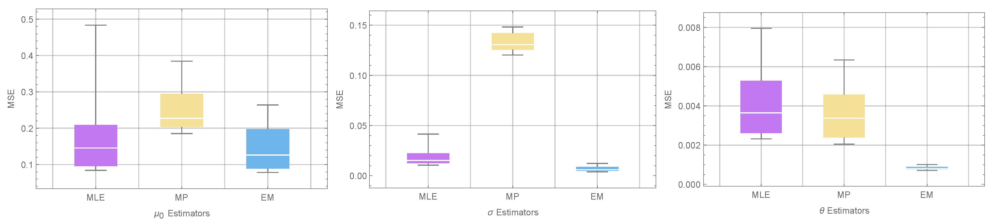
5.1. Monte Carlo Simulation Study

Based on theoretical principles, it is not possible to directly compare various estimation methods or censoring schemes. Therefore, the purpose of this section is to evaluate the performance of several estimates that were discussed in previous sections using Monte Carlo simulations. The assessment of point estimates is based on their mean square error (MSE) and relative absolute bias (RAB), while the evaluation of interval estimates is based on their coverage probability (CP) and average width (AW). These measures provide insights into the accuracy and precision of the estimates.
To simulate data under progressive type-I interval censoring, we utilize the Aggarwala algorithm (Aggarwala et al. [12]) for a given set of parameters including the specified stress level S i , the sample sizes n i , and the number of subintervals m i . We also consider prefixed inspection times and censoring schemes. Under each stress level S i , i = 1 , 2 , , k , starting with a sample of size n i , which is subjected to a life test at time t i 0 = 0 , we simulate the number of failed items X i j for each subinterval ( t i ( j 1 ) , t i j ] as follows: Let X i 0 = 0 and R i 0 = 0 and for j = 1 , 2 , , m i
X i j | X i ( j 1 ) , R i ( j 1 ) , , X i 0 , R i 0 Bin n i l = 1 j 1 X i l + R i l , Φ τ i j Φ τ i ( j 1 ) 1 Φ τ i j , R i j = p i j × n i l = 1 j 1 X i l + R i l X i j .
In the simulation study, we examine three distinct removal schemes, denoted as p 1 , p 2 , and p 3 , each characterized by different probabilities of removing items during intermediate inspection times where p 1 = ( 0.25 , 0.25 , 0 , 0 , 1 ) , p 2 = ( 0 , 0 , 0.25 , 0.25 , 1 ) , and p 3 = ( 0 , 0 , 0 , 0 , 1 ) . The third Scheme, p 3 , resembles a conventional interval censoring scheme, where no removals occur during the intermediate inspection times. In addition to the regular stress level S 0 = 50 , we include four stress levels: S 1 = 60 , S 2 = 70 , S 3 = 80 , and S 4 = 90 . These stress levels represent different levels of intensity or severity in the testing process. Additionally, for each stress level S i , we incorporate the same inspection times to account for varying durations of observation. The inspection times included are t i 1 = 3 , t i 2 = 5 , t i 3 = 9 , t i 4 = 15 , and t i 5 = 25 . These inspection times correspond to specific intervals during which the items are assessed or observed.
Furthermore, we consider various sample sizes to assess the impact of the number of items tested. The sample sizes considered are n = 40 , n = 60 , n = 80 , and n = 100 . These different sample sizes allow us to investigate the influence of the number of tested items on the estimation performance. The generated data follows a log-normal distribution with true parameters values μ 0 = 2 , σ = 1 , and θ = 0.95 .
For the Bayesian analyses, informative priors are employed with specific hyperparameters. The hyperparameters are chosen such that the prior means correspond to the true parameter values. The hyperparameters are set as follows: λ 1 = 2 , μ 1 = 0.1 , λ 2 = 100 , and μ 2 = 100 . The T-K BEs are calculated under the SE loss function. On the other hand, the MCMC BEs are computed using the SE loss function as well as the LINEX loss function with different values of ν ( 2 , 0.001, and 2) and the GE loss function with different values of κ ( 2 , 0.001, and 2).
In Table 1, the MSE and RAB values are provided for the classical estimators of the parameters. The table clearly demonstrates that the EM estimators outperform the MLE and MP estimators in terms of having the lowest MSE and RAB values. This indicates that the EM estimators provide more accurate and less biased parameter estimates compared to their counterparts, as clearly demonstrated in Figure 1.
In Table 2, the MSE and RAB values are presented for the BEs of the parameters, specifically under the SE loss function. The table includes results obtained using the T-K and MCMC techniques. The tabulated results indicate that the performance of the two methods under different schemes is almost identical, as visually depicted in Figure 2 as well. Suggesting that both T-K and MCMC methods yield similar results in terms of MSE and RAB values.
Additionally, in Table 3 and Table 4, the MSE and RAB values are presented for the MCMC BEs of the parameters for three distinct choices of the shape parameter for the LINEX and GE loss functions. Table 3 corresponds to the LINEX. Based on the tabulated results, we can conclude that, for the parameters μ 0 and σ under the LINEX loss function, the MCMC BE shows higher accuracy when the parameter ν is set to 2. This means that for a specific value of ν (in this case, ν = 2 ), the MCMC BE provides more precise and reliable estimates for μ 0 and σ under the LINEX loss function compared to other values of ν . On the other hand, for the parameter θ under the same LINEX loss function, the MCMC BE performs better (i.e., shows higher accuracy) when ν is set to 2 .
Moreover, when considering the GE loss function, the MCMC BE of μ 0 shows higher accuracy when κ is assigned a value of 2. Similarly, for the parameter σ , the MCMC BE exhibits better performance in terms of lower MSE and RAB values when κ is set to 0.001. On the other hand, for the parameter θ , the MCMC BE demonstrates better performance when κ is set to 2 .
Moreover, Table 5 presents the AWs and coverage probabilities (CPs) of the 95 % asymptotic and Bayesian credible CIs for the parameters μ 0 , σ , and θ . The table clearly indicates that the Bayesian credible CIs have narrower widths compared to the asymptotic CIs. This suggests that the Bayesian credible CIs provide more precise and tighter estimation intervals for the parameters. Also, the Bayesian credible CIs demonstrate better overall performance, as indicated by the higher coverage probabilities, implying that they achieve a higher proportion of correctly capturing the true parameter values within the confidence intervals.
Based on the tabulated results in Table 1, Table 2, Table 3, Table 4 and Table 5, the following general concluding remarks can be drawn:
  • For a fixed censoring scheme, the trend observed in the tabulated results indicates that as the sample size n increases, the MSE and RAB values of all estimates decrease. This trend aligns with the statistical theory, which suggests that larger sample sizes tend to result in more accurate parameter estimates.
  • The Bayesian estimators consistently outperform the MLEs, EM estimators, and MP estimators in terms of MSE and RAB values. This highlights the superior performance of the Bayesian approach in estimation tasks.
  • Among the different progressive censoring schemes p 1 , p 2 , and p 3 , all the estimates obtained under scheme p 3 (traditional type-I interval censoring) exhibit the smallest MSE and RAB values compared to schemes p 1 and p 2 . This result is in line with expectations, as longer testing duration and lower censoring rates generally lead to more accurate parameter estimation.
  • The BEs of the parameters under the LINEX loss function display higher accuracy compared to the estimators under the SE and GE loss functions.
These conclusions provide insights into the behavior and performance of different estimation methods, sample sizes, censoring schemes, and loss functions based on the tabulated results.

5.2. Data Analysis

The life data from steel samples, which were randomly divided into groups of 20 items, indicates that each group experienced varying levels of stress intensity (Kimber [38]; Lawless [39]). Cui et al. [40] demonstrated that the data could be well described by a log-normal distribution. Our analysis specifically focused on the data obtained from stress levels ranging from 35 to 36 MPa, with a normal stress level set at 30 MPa. To facilitate convenience, the data is replicated in Table 6 for easy reference.
A progressively type-I interval censored sample is generated randomly from this dataset, taking into account the predetermined inspection times t i j = j * 50 , under the scheme p = ( 0 , 0 , 0 , 0 , 1 ) . The resulting simulated sample is presented in Table 7.
Table 8, Table 9, Table 10, Table 11 and Table 12 provide the corresponding point and interval estimates for the parameters μ 0 , σ , and θ . Non-informative priors are utilized to obtain the BEs since there is insufficient prior information available.

6. Conclusions

This article discusses statistical analysis in the context of progressive type-I interval censoring for the log-normal distribution in a CS-ALT setting. Both classical and Bayesian inferential procedures are applied to estimate the unknown parameters. To approximate the MLEs of the model parameters, the EM algorithm and mid-point approximation method are employed. For the Bayesian approach, the BEs are obtained based on different loss functions, namely the SE, LINEX, and GE loss functions. The Tierney–Kadane and MCMC methods are used to obtain approximate BEs. Additionally, the article derives the asymptotic confidence intervals based on the normality assumption of the MLEs and the Bayesian credible intervals using the MCMC procedure. The performance of the different estimation methods is evaluated through a simulation study. The results indicate that the BEs perform well based on measures such as mean squared error and relative absolute bias of the estimates.
While this article focuses on CS-ALT with progressive type-I interval censoring and the log-normal distribution, the same methodology can be applied to other lifetime distributions under different censoring schemes as well.
Overall, this article provides a comprehensive analysis of statistical procedures for estimating parameters in CS-ALT with progressive type-I interval censoring, specifically for the log-normal distribution.

Author Contributions

Conceptualization, A.E.-R.M.A.E.-R. and M.S.; methodology, M.S.; software, M.S. and A.E.-R.M.A.E.-R.; validation, X.L., M.S. and M.H.; formal analysis, M.S.; investigation, M.S.; resources, M.S.; data curation, M.S.; writing—original draft preparation, M.S.; writing—review and editing, M.S.; visualization, M.S.; supervision, X.L. project administration, M.H.; funding acquisition, M.H. All authors have read and agreed to the published version of the manuscript.

Funding

This research received no external funding.

Data Availability Statement

The article incorporates the numerical data that were utilized to substantiate the findings of the study.

Acknowledgments

The third author extends her appreciation to the Deanship of Scientific Research at King Khalid University for funding this work through a research groups program under grant RGP2/310/44.

Conflicts of Interest

The authors declare no conflict of interest.

References

  1. Nelson, W.B. Accelerated Testing: Statistical Models, Test Plans, and Data Analysis; John Wiley & Sons: New York, NY, USA, 2009; Volume 344. [Google Scholar]
  2. Meeker, W.Q.; Escobar, L.A. Statistical Methods for Reliability Data; John Wiley & Sons: New York, NY, USA, 2014. [Google Scholar]
  3. Bagdonavicius, V.; Nikulin, M. Accelerated Life Models: Modeling and Statistical Analysis; Chapman and Hall: Boca Raton, FL, USA, 2001. [Google Scholar]
  4. Limon, S.; Yadav, O.P.; Liao, H. A literature review on planning and analysis of accelerated testing for reliability assessment. Qual. Reliab. Eng. Int. 2017, 33, 2361–2383. [Google Scholar] [CrossRef]
  5. Zheng, G. A characterization of the factorization of hazard function by the Fisher information under type-II censoring with application to the Weibull family. Stat. Probab. Lett. 2001, 52, 249–253. [Google Scholar] [CrossRef]
  6. Xu, H.; Fei, H. Approximated optimal designs for a simple step-stress model with type-II censoring, and Weibull distribution. In Proceedings of the 2009 8th International Conference on Reliability, Maintainability and Safety, Chengdu, China, 20–24 July 2009; IEEE: Piscataway, NJ, USA, 2009; pp. 1203–1207. [Google Scholar]
  7. Wu, W.; Wang, B.X.; Chen, J.; Miao, J.; Guan, Q. Interval estimation of the two-parameter exponential constant stress accelerated life test model under type-II censoring. Qual. Technol. Quant. Manag. 2022, 1–12. [Google Scholar] [CrossRef]
  8. Nelson, W.; Kielpinski, T.J. Theory for optimum censored accelerated life tests for normal and lognormal life distributions. Technometrics 1976, 18, 105–114. [Google Scholar] [CrossRef]
  9. Bai, D.S.; Kim, M.S. Optimum simple step-stress accelerated life tests for Weibull distribution and type I censoring. Nav. Res. Logist. (NRL) 1993, 40, 193–210. [Google Scholar] [CrossRef]
  10. Tang, L.; Goh, T.; Sun, Y.; Ong, H. Planning accelerated life tests for censored two-parameter exponential distributions. Nav. Res. Logist. (NRL) 1999, 46, 169–186. [Google Scholar] [CrossRef]
  11. Balakrishnan, N.; Aggarwala, R. Progressive Censoring: Theory, Methods, and Applications, 1st ed.; Statistics for Industry and Technology; Birkhäuser: Basel, Switzerland, 2000. [Google Scholar]
  12. Aggarwala, R. Progressive interval censoring: Some mathematical results with applications to inference. Commun. Stat. Theory Methods 2001, 30, 1921–1935. [Google Scholar] [CrossRef]
  13. Lodhi, C.; Tripathi, Y.M. Inference on a progressive type-I interval censored truncated normal distribution. J. Appl. Stat. 2020, 47, 1402–1422. [Google Scholar] [CrossRef]
  14. Singh, S.; Tripathi, Y.M. Estimating the parameters of an inverse Weibull distribution under progressive type-I interval censoring. Stat. Pap. 2018, 59, 21–56. [Google Scholar] [CrossRef]
  15. Chen, D.G.; Lio, Y.; Jiang, N. Lower confidence limits on the generalized exponential distribution percentiles under progressive type-I interval censoring. Commun. Stat.-Simul. Comput. 2013, 42, 2106–2117. [Google Scholar] [CrossRef]
  16. Arabi Belaghi, R.; Noori Asl, M.; Singh, S. On estimating the parameters of the BurrXII model under progressive type-I interval censoring. J. Stat. Comput. Simul. 2017, 87, 3132–3151. [Google Scholar] [CrossRef]
  17. Abd El-Raheem, A.M. Optimal design of multiple constant-stress accelerated life testing for the extension of the exponential distribution under type-II censoring. J. Comput. Appl. Math. 2021, 382, 113094. [Google Scholar] [CrossRef]
  18. Abd El-Raheem, A.M. Optimal design of multiple accelerated life testing for generalized half-normal distribution under type-I censoring. J. Comput. Appl. Math. 2020, 368, 112539. [Google Scholar] [CrossRef]
  19. Abd El-Raheem, A.M. Optimal plans of constant-stress accelerated life tests for extension of the exponential distribution. J. Test. Eval. 2018, 47, 1586–1605. [Google Scholar] [CrossRef]
  20. Sief, M.; Liu, X.; Abd El-Raheem, A.M. Inference for a constant-stress model under progressive type-I interval censored data from the generalized half-normal distribution. J. Stat. Comput. Simul. 2021, 91, 3228–3253. [Google Scholar] [CrossRef]
  21. Feng, X.; Tang, J.; Tan, Q.; Yin, Z. Reliability model for dual constant-stress accelerated life test with Weibull distribution under Type-I censoring scheme. Commun. Stat. Theory Methods 2022, 51, 8579–8597. [Google Scholar] [CrossRef]
  22. Balakrishnan, N.; Castilla, E.; Ling, M.H. Optimal designs of constant-stress accelerated life-tests for one-shot devices with model misspecification analysis. Qual. Reliab. Eng. Int. 2022, 38, 989–1012. [Google Scholar] [CrossRef]
  23. Nassar, M.; Dey, S.; Wang, L.; Elshahhat, A. Estimation of Lindley constant-stress model via product of spacing with Type-II censored accelerated life data. Commun. Stat. Simul. Comput. 2021, 1–27. [Google Scholar] [CrossRef]
  24. Serfling, R. Efficient and robust fitting of lognormal distributions. N. Am. Actuar. J. 2002, 6, 95–109. [Google Scholar] [CrossRef] [Green Version]
  25. Punzo, A.; Bagnato, L.; Maruotti, A. Compound unimodal distributions for insurance losses. Insur. Math. Econ. 2018, 81, 95–107. [Google Scholar] [CrossRef]
  26. Limpert, E.; Stahel, W.A.; Abbt, M. Log-normal distributions across the sciences: Keys and clues: On the charms of statistics, and how mechanical models resembling gambling machines offer a link to a handy way to characterize log-normal distributions, which can provide deeper insight into variability and probability-normal or log-normal: That is the question. BioScience 2001, 51, 341–352. [Google Scholar]
  27. Dempster, A.P.; Laird, N.M.; Rubin, D.B. Maximum likelihood from incomplete data via the EM algorithm. J. R. Stat. Soc. Ser. B (Methodol.) 1977, 39, 1–22. [Google Scholar]
  28. McLachlan, G.J.; Krishnan, T. The EM Algorithm and Extensions, 2nd ed.; Wiley: New York, NY, USA, 2008; pp. 159–218. [Google Scholar]
  29. Little, R.J.A.; Rubin, D.B. Incomplete data. In Encyclopedia of Statistical Sciences; Kotz, S., Johnson, N.L., Eds.; Wiley: New York, NY, USA, 1983; Volume 4, pp. 46–53. [Google Scholar]
  30. Ng, H.; Chan, P.; Balakrishnan, N. Estimation of parameters from progressively censored data using EM algorithm. Comput. Stat. Data Anal. 2002, 39, 371–386. [Google Scholar] [CrossRef]
  31. Ng, H.K.T.; Wang, Z. Statistical estimation for the parameters of Weibull distribution based on progressively type-I interval censored sample. J. Stat. Comput. Simul. 2009, 79, 145–159. [Google Scholar] [CrossRef]
  32. Louis, T.A. Finding the observed information matrix when using the EM algorithm. J. R. Stat. Soc. Ser. B (Methodol.) 1982, 44, 226–233. [Google Scholar]
  33. Arnold, B.C.; Press, S. Bayesian inference for Pareto populations. J. Econom. 1983, 21, 287–306. [Google Scholar] [CrossRef]
  34. Smith, A.F.; Roberts, G.O. Bayesian computation via the Gibbs sampler and related Markov chain Monte Carlo methods. J. R. Stat. Soc. Ser. B (Methodol.) 1993, 55, 3–23. [Google Scholar] [CrossRef]
  35. Metropolis, N.; Rosenbluth, A.W.; Rosenbluth, M.N.; Teller, A.H.; Teller, E. Equation of State Calculations by Fast Computing Machines. J. Chem. Phys. 1953, 21, 1087. [Google Scholar] [CrossRef] [Green Version]
  36. Hastings, W.K. Monte Carlo sampling methods using Markov chains and their applications. Biometrika 1970, 57, 97–109. [Google Scholar] [CrossRef]
  37. Tierney, L.; Kadane, J.B. Accurate approximations for posterior moments and marginal densities. J. Am. Stat. Assoc. 1986, 81, 82–86. [Google Scholar] [CrossRef]
  38. Kimber, A. Exploratory data analysis for possibly censored data from skewed distributions. J. R. Stat. Soc. Ser. C Appl. Stat. 1990, 39, 21–30. [Google Scholar] [CrossRef]
  39. Lawless, J.F. Statistical Models and Methods for Lifetime Data, 2nd ed.; Wiley Series in Probability and Statistics; Wiley-Interscience: Hoboken, NJ, USA, 2002. [Google Scholar]
  40. Cui, W.; Yan, Z.Z.; Peng, X.Y.; Zhang, G.M. Reliability analysis of log-normal distribution with nonconstant parameters under constant-stress model. Int. J. Syst. Assur. Eng. Manag. 2022, 13, 818–831. [Google Scholar] [CrossRef]
Figure 1. Comparison of classical estimators: MSE values for different parameters estimators.
Axioms 12 00710 g001
Figure 2. Comparison of BEs under SE loss function: MSE values for different parameters estimators.
Axioms 12 00710 g002
Table 1. The MSEs of the classical estimates for μ 0 , σ , and θ , along with their corresponding RAB values, are provided within brackets.
μ 0 σ θ
nCSMLEMPEMMLEMPEMMLEMPEM
40 p 1 0.483450.384370.263900.041590.148220.012220.007950.006340.00101
(0.18292)(0.27032)(0.17876)(0.13258)(0.37055)(0.08386)(0.06153)(0.05826)(0.02718)
p 2 0.276760.329290.219910.024340.132260.011400.006940.005850.00100
(0.18075)(0.25572)(0.16967)(0.12104)(0.35167)(0.08338)(0.06065)(0.05550)(0.02732)
p 3 0.196530.301320.202880.023510.127770.010300.005100.004300.00093
(0.16592)(0.24502)(0.16894)(0.12087)(0.34676)(0.07970)(0.05530)(0.05445)(0.02637)
60 p 1 0.221570.287660.191520.021180.143850.007180.005460.004850.00085
(0.15658)(0.24018)(0.15182)(0.11214)(0.37033)(0.06819)(0.05385)(0.05231)(0.02601)
p 2 0.162010.237240.122690.017230.130640.006620.003270.004030.00083
(0.14385)(0.21936)(0.13442)(0.10188)(0.35426)(0.06392)(0.04689)(0.04914)(0.02549)
p 3 0.132780.190470.118190.014490.123240.006730.003990.002900.00081
(0.13819)(0.12115)(0.11269)(0.09458)(0.34376)(0.06484)(0.05024)(0.04505)(0.02521)
80 p 1 0.158220.245150.135220.015800.142250.005440.004010.003380.00079
(0.13113)(0.22474)(0.12670)(0.09824)(0.37088)(0.05839)(0.04583)(0.04441)(0.02553)
p 2 0.129000.208860.129760.013050.130660.005230.003300.003370.00081
(0.12442)(0.20909)(0.12596)(0.08884)(0.35602)(0.05533)(0.04412)(0.04229)(0.02565)
p 3 0.094200.217110.090830.012350.120270.005100.002510.002320.00079
(0.12033)(0.21439)(0.11865)(0.08875)(0.34112)(0.05743)(0.04272)(0.04124)(0.02501)
100 p 1 0.097230.212920.087040.012750.141670.004710.002730.002450.00077
(0.12076)(0.21116)(0.11555)(0.08828)(0.37121)(0.05429)(0.04357)(0.04163)(0.02500)
p 2 0.086920.198480.078870.010620.129060.004320.002370.002070.00075
(0.11444)(0.20703)(0.11012)(0.08211)(0.35498)(0.05233)(0.04050)(0.03829)(0.02471)
p 3 0.084070.185210.078260.010550.120620.003910.002320.002050.00071
(0.11034)(0.19890)(0.10737)(0.08157)(0.34267)(0.04979)(0.03967)(0.03762)(0.02363)
Table 2. The MSEs of the BEs evaluated using the SE loss function, along with their corresponding RABs (shown in parentheses).
μ 0 σ θ
nCST-KMCMCT-KMCMCT-KMCMC
40 p 1 0.000960.000980.002870.002860.004300.00130
(0.01220)(0.01233)(0.04270)(0.04257)(0.05445)(0.03025)
p 2 0.000920.000950.002630.002630.001280.00130
(0.01218)(0.01225)(0.04125)(0.04125)(0.03001)(0.02917)
p 3 0.000830.000840.002440.002440.001270.00103
(0.01152)(0.01161)(0.03925)(0.03933)(0.02888)(0.02729)
60 p 1 0.000760.000770.002690.002700.000880.00089
(0.01104)(0.01106)(0.04187)(0.04198)(0.02477)(0.02489)
p 2 0.000720.000730.002400.002400.000740.00075
(0.01062)(0.01072)(0.03883)(0.03890)(0.02272)(0.02290)
p 3 0.000630.000640.002340.002350.000700.00071
(0.00999)(0.01008)(0.03861)(0.03861)(0.02210)(0.02219)
80 p 1 0.000590.000600.002410.002420.000730.00074
(0.00968)(0.00972)(0.03861)(0.03876)(0.02237)(0.02247)
p 2 0.000550.000570.002360.002360.000630.00063
(0.00930)(0.00938)(0.03897)(0.03894)(0.02099)(0.02105)
p 3 0.000530.000540.002090.002090.000600.00060
(0.00908)(0.00914)(0.03675)(0.03679)(0.02030)(0.02036)
100 p 1 0.000420.000460.002310.002310.000560.00056
(0.00802)(0.00900)(0.03885)(0.03889)(0.01983)(0.01985)
p 2 0.000390.000430.002120.002160.000500.00050
(0.00798)(0.00816)(0.03672)(0.03689)(0.01886)(0.01888)
p 3 0.000340.000410.001960.002140.000470.00047
(0.00735)(0.00806)(0.03522)(0.03564)(0.01806)(0.01815)
Table 3. The MSEs of the BEs evaluated under LINEX loss function with different values of ν ( 2 , 0.001, and 2), along with their corresponding RABs (shown in parentheses).
μ 0 σ θ
nCS ν = 2 ν = 0.001 ν = 2 ν = 2 ν = 0.001 ν = 2 ν = 2 ν = 0.001 ν = 2
40 p 1 0.001260.000980.000850.002930.002860.002840.001260.001300.00134
(0.01422)(0.01233)(0.01150)(0.04296)(0.04257)(0.04248)(0.02983)(0.03025)(0.03073)
p 2 0.001190.000950.000860.002770.002630.002550.001250.001300.00136
(0.01376)(0.01225)(0.01179)(0.04233)(0.04125)(0.04061)(0.02866)(0.02917)(0.02973)
p 3 0.001060.000840.000780.002530.002440.002410.001010.001060.00111
(0.01314)(0.01161)(0.01121)(0.04012)(0.03933)(0.03902)(0.02705)(0.02761)(0.02821)
60 p 1 0.001050.000770.000650.002820.002700.002650.000860.000890.00092
(0.01306)(0.01105)(0.01018)(0.04273)(0.04198)(0.04161)(0.02455)(0.02489)(0.02527)
p 2 0.000990.000730.000640.002540.002400.002330.000730.000750.00078
(0.01267)(0.01072)(0.01004)(0.03977)(0.03890)(0.03822)(0.02254)(0.02290)(0.02330)
p 3 0.000870.000640.000570.002490.002350.002290.000690.000710.00073
(0.01177)(0.01008)(0.00962)(0.03974)(0.03861)(0.03857)(0.02185)(0.02219)(0.02257)
80 p 1 0.000880.000600.000490.002460.002360.002330.000720.000740.00076
(0.01198)(0.00972)(0.00884)(0.03993)(0.03894)(0.03862)(0.02224)(0.02247)(0.02273)
p 2 0.000810.000570.000490.002560.002420.002360.000610.000630.00065
(0.01142)(0.00938)(0.00883)(0.039810(0.03876)(0.03847)(0.02080)(0.02105)(0.02132)
p 3 0.000780.000540.000480.002220.002090.002050.000590.000600.00062
(0.01113)(0.00914)(0.00871)(0.03772)(0.03679)(0.03656)(0.02010)(0.02036)(0.02065)
100 p 1 0.000730.000500.000450.002310.002160.002140.000550.000560.00057
(0.01096)(0.00901)(0.00867)(0.03677)(0.03564)(0.03557)(0.01964)(0.01985)(0.02008)
p 2 0.000700.000430.000350.002430.002310.002290.000490.000500.00051
(0.01055)(0.00816)(0.00761)(0.03972)(0.03889)(0.03885)(0.01865)(0.01888)(0.01913)
p 3 0.000660.000410.000340.002270.002140.002120.000460.000470.00049
(0.01040)(0.00806)(0.00746)(0.03813)(0.03689)(0.03663)(0.01797)(0.01815)(0.01834)
Table 4. The MSEs of the BEs evaluated under GE loss function with different values of κ ( 2 , 0.001, and 2), along with their corresponding RABs (shown in parentheses).
μ 0 σ θ
nCS κ = 2 κ = 0.001 κ = 2 κ = 2 κ = 0.001 κ = 2 κ = 2 κ = 0.001 κ = 2
40 p 1 0.001940.001870.001850.002880.002860.002880.001270.001330.00141
(0.01338)(0.01307)(0.01211)(0.04262)(0.04260)(0.04285)(0.02999)(0.03053)(0.03114)
p 2 0.001030.000930.000870.002680.002600.002570.001270.001320.00139
(0.01269)(0.01205)(0.01164)(0.04164)(0.04097)(0.04075)(0.02886)(0.02949)(0.03020)
p 3 0.000990.000910.000870.002200.002150.002210.001030.001080.00115
(0.01252)(0.01203)(0.01184)(0.03596)(0.03566)(0.03631)(0.02728)(0.02794)(0.02868)
60 p 1 0.000880.000810.000780.002740.002680.002680.000870.000910.00094
(0.01189)(0.01141)(0.01124)(0.04219)(0.04185)(0.04189)(0.02469)(0.02511)(0.02558)
p 2 0.000780.000690.000650.002450.002370.002360.000740.000770.00080
(0.01107)(0.01044)(0.01013)(0.03915)(0.03878)(0.03890)(0.02269)(0.02313)(0.02361)
p 3 0.000680.000610.000580.002390.002320.002330.000700.000720.00075
(0.01035)(0.00988)(0.00968)(0.03895)(0.03846)(0.03860)(0.02199)(0.02240)(0.02286)
80 p 1 0.000820.000720.000670.002380.002350.002390.000730.000750.00077
(0.01145)(0.01073)(0.01033)(0.03923)(0.03881)(0.03904)(0.02233)(0.02262)(0.02294)
p 2 0.000610.000530.000500.002460.002390.002400.000620.000640.00066
(0.00976)(0.00910)(0.00884)(0.03907)(0.03865)(0.03890)(0.02126)(0.02120)(0.02153)
p 3 0.000580.000510.000480.002120.002070.002110.000590.000610.00063
(0.00949)(0.00889)(0.00869)(0.03701)(0.03672)(0.03709)(0.02090)(0.02052)(0.02086)
100 p 1 0.000650.000550.000500.002460.002430.002460.000550.000570.00058
(0.01015)(0.00937)(0.00895)(0.03955)(0.03921)(0.03942)(0.01973)(0.01998)(0.02025)
p 2 0.000480.000400.000360.002340.002310.002370.000490.000510.00052
(0.00857)(0.00788)(0.00763)(0.03907)(0.03889)(0.03950)(0.01875)(0.01902)(0.01931)
p 3 0.000450.000380.000340.001180.001130.001190.000470.000480.00050
(0.00850)(0.00772)(0.00746)(0.03723)(0.03682)(0.03718)(0.01804)(0.01825)(0.01849)
Table 5. Comparison of AWs and CPs of 95% asymptotic and Bayesian Credible CIs for μ 0 , σ , and θ .
μ 0 σ θ
nCSACIBCIACIBCIACIBCI
40 p 1 2.32530.38190.74810.34160.37760.1604
0.9880.9980.9500.9980.9760.976
p 2 2.02580.38240.63220.33160.33030.1541
0.9690.9750.9121.0000.9460.993
p 3 2.08780.38180.62150.32800.35740.1542
0.9791.0000.9160.9660.9680.968
60 p 1 1.80850.37850.58480.32380.29480.1352
0.9720.9490.9480.9780.9620.977
p 2 1.58940.37730.51420.31170.27100.1304
0.9760.9770.9400.9940.9630.982
p 3 1.52860.37710.48480.30610.25530.1290
0.9690.9980.9280.9990.9480.988
80 p 1 1.51690.37520.50410.30880.25370.1207
0.9730.9450.9430.9990.9620.972
p 2 1.34550.37280.44560.29530.22660.1162
0.9750.9850.9400.9950.9580.983
p 3 1.32700.37310.42010.28780.22840.1153
0.9671.0000.9320.9960.9610.982
100 p 1 1.25120.37180.44430.29500.21590.1108
0.9720.9540.9380.9970.9530.982
p 2 1.17320.36890.40050.28100.20460.1069
0.9690.9500.9420.9950.9570.984
p 3 1.13520.36810.36920.27200.19610.1057
0.9600.9940.9050.9880.9480.985
Table 6. Data on steel specimens’ life under different stress levels.
Stress (MPa)Failure Times
35230, 169, 178, 271, 129, 568, 115, 280, 305, 326, 1101, 285, 734, 177, 493, 218, 342, 431, 143, 381
36173, 218, 162, 288, 394, 585, 295, 262, 127, 151, 181, 209, 141, 186, 309, 192, 117, 203, 198, 255
37141, 143, 98, 122, 110, 132, 194, 155, 104, 83, 125, 165, 146, 100, 318, 136, 200, 201, 251, 111
38100, 90, 59, 80, 128, 117, 177, 98, 158, 107, 125, 118, 99, 186, 66, 132, 97, 87, 69, 109
Table 7. The progressively type-I interval censored sample.
Stress Level X ij R ij
S 1 (0, 0, 3, 3, 1)(0, 0, 0, 0, 13)
S 2 (0, 0, 3, 7, 3)(0, 0, 0, 0, 7)
S 3 (0, 3, 10, 4, 1)(0, 0, 0, 0, 2)
S 4 (0, 10, 7, 3, 0)(0, 0, 0, 0, 0)
Table 8. The classical point estimates for μ 0 , σ , and θ of the real data.
μ 0 σ θ
MLEMPEMMLEMPEMMLEMPEM
9.6536 × 10 12 1.49323 × 10 12 9.65582 × 10 11 6.537586.557326.529341.8055 × 10 13 2.11906 × 10 12 1.8055 × 10 13
Table 9. The BEs under the SE loss function of the real data.
μ 0 σ θ
T-KMCMCT-KMCMCT-KMCMC
9.9638 × 10 10 9.6536 × 10 12 6.519246.596273.2541 × 10 14 4.54567 × 10 13
Table 10. The BEs under LINEX loss function with different values of ν for the real data.
μ 0 σ θ
ν = 2 ν = 0 . 001 ν = 2 ν = 2 ν = 0 . 001 ν = 2 ν = 2 ν = 0 . 001 ν = 2
9.58256 × 10 12 2.22045 × 10 13 9.5825 × 10 12 7.173276.596056.244094.53526 × 10 13 1.0147 × 10 14 4.53415 × 10 13
Table 11. The BEs under GE loss function with different values of κ for the real data.
μ 0 σ θ
κ = 2 κ = 0 . 001 κ = 2 κ = 2 κ = 0 . 001 κ = 2 κ = 2 κ = 0 . 001 κ = 2
9.6536 × 10 12 9.6536 × 10 12 9.6536 × 10 12 6.628286.564826.50375.33591 × 10 13 3.36419 × 10 13 5.49065 × 10 13
Table 12. The ACI and BCI of μ 0 , σ , and θ for the real data.
μ 0 σ θ
ACIBCIACIBCIACIBCI
( 0.221022 , 0.221022)( 0.05928 , 0.201439)(5.2699, 7.80526)(5.48794, 8.04582)(1.8055 × 10 13 , 1.74424 × 10 12 )(2.8756 × 10 14 , 9.93455 × 10 13 )
Disclaimer/Publisher’s Note: The statements, opinions and data contained in all publications are solely those of the individual author(s) and contributor(s) and not of MDPI and/or the editor(s). MDPI and/or the editor(s) disclaim responsibility for any injury to people or property resulting from any ideas, methods, instructions or products referred to in the content.

